A New Method for Predicting Pile Accumulated Deformation and Stiffness of Evolution Under Long-Term Inclined Cyclic Loading

Abstract

Piles in marine environments are subjected to various loads of differing magnitudes and directions, and their long-term stability has attracted much attention. Most research focuses on lateral cyclic loading; there are few full-scale tests that consider the effects of cyclic loading at different inclined angles. A long-term inclined cyclic loading strategy was used to carry out laboratory tests to study different inclined angles on the pile. The results show that a smaller inclined angle (θ_L) or a larger pile–soil relative stiffness (T/L) results in wider and deeper sediment subsidence after 10,000 cycles. As θ_L increases from 0° to 80°, the peak displacement at the pile head during the first load decreases, while the accumulated displacement initially decreases and then increases. For slender piles, the normalized inclined cyclic loading stiffness (k_lN/k_l1) and unloading stiffness (k_uN/k_u1) first decrease and then increase. For semi-rigid piles, both k_lN/k_l1 and k_uN/k_u1 gradually decrease. On the other hand, as θ_L increases, k_lN/k_l1 and k_uN/k_u1 increased more sharply in the initial stage, with a quicker transition from rapid growth to stability. At θ_L = 80°, peak values are reached early during the initial loading phase. Based on this, prediction formulas for inclined cyclic cumulative displacement, loading stiffness, and unloading stiffness were established and verified.

1. Introduction

As the most commonly used foundation type, piles are widely used in many offshore wind farms, cross-sea bridges, ports, piers, and other marine engineering projects [1,2,3]. These foundations, embedded in the seabed, are directly related to the safety and stability of structures and are the most critical aspect of the design process [4,5]. Piles in complex marine environments need to bear loads caused by sea waves, waves, and currents [6,7], and the size and direction of the loads are not fixed, and they have the characteristics of long-term circulation. There have been many important research results on pile cumulative deformation under lateral cyclic load. Hettler et al. [8] and Lin et al. [9], respectively, conducted in situ tests on the lateral cyclic loading of monopile foundations for offshore wind turbines and proposed cumulative deformation prediction formulas. However, in situ tests are challenging and costly [10,11,12,13]. Therefore, most researchers have adopted laboratory tests to conduct related studies. Leblanc et al. [14,15] found that in lateral cyclic loading tests on rigid piles in sandy soils, cyclic unloading stiffness is only related to cycle number (N), not on load characteristics or soil parameters. Lin Jingyang [16] and Wang Yang et al. [17] conducted extensive laboratory tests on piles under lateral cyclic loading, analyzing the relationship between the hysteresis curves and the N, and proposed a cumulative displacement prediction formula considering factors such as the characteristics of cyclic loading and the pile–soil relative stiffness. Some scholars, such as Rathod et al. [18], Liang et al. [19], Li et al. [20], and Chen et al. [21], also conducted lateral cyclic loading tests of monopiles and developed cumulative displacement calculation models. Meanwhile, some researchers have used theoretical methods to predict the mechanical behavior of monopiles under lateral loads [8,22,23]. However, the above existing experimental studies are limited to the cumulative deformation and bearing characteristics of piles under lateral static and cyclic loads. In contrast, there is still a lack of in-depth analysis on the research of piles under cyclic loads from different inclined angles.

This study aims to further investigate the effects of different inclined angles on the evolution characteristics of cumulative displacement, loading, and unloading stiffness for piles under inclined cyclic loading. Using a cyclic loading apparatus, inclined cyclic loading model tests on piles in sandy soils were conducted. Inclined cyclic normalized prediction formulas for cumulative displacement, loading, and unloading stiffness were proposed. The research findings aim to provide experimental evidence for the design methods of pile foundation cumulative deformation under long-term cyclic loading.

2. Model Overview

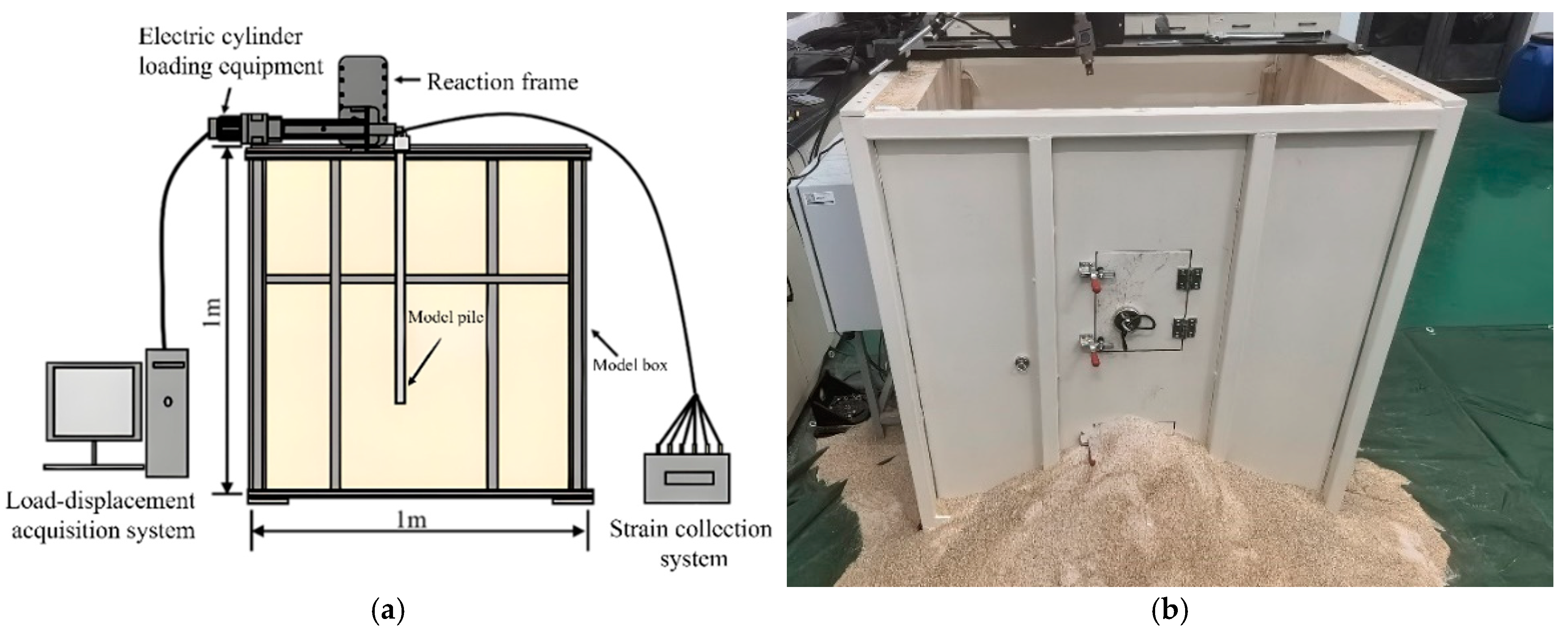
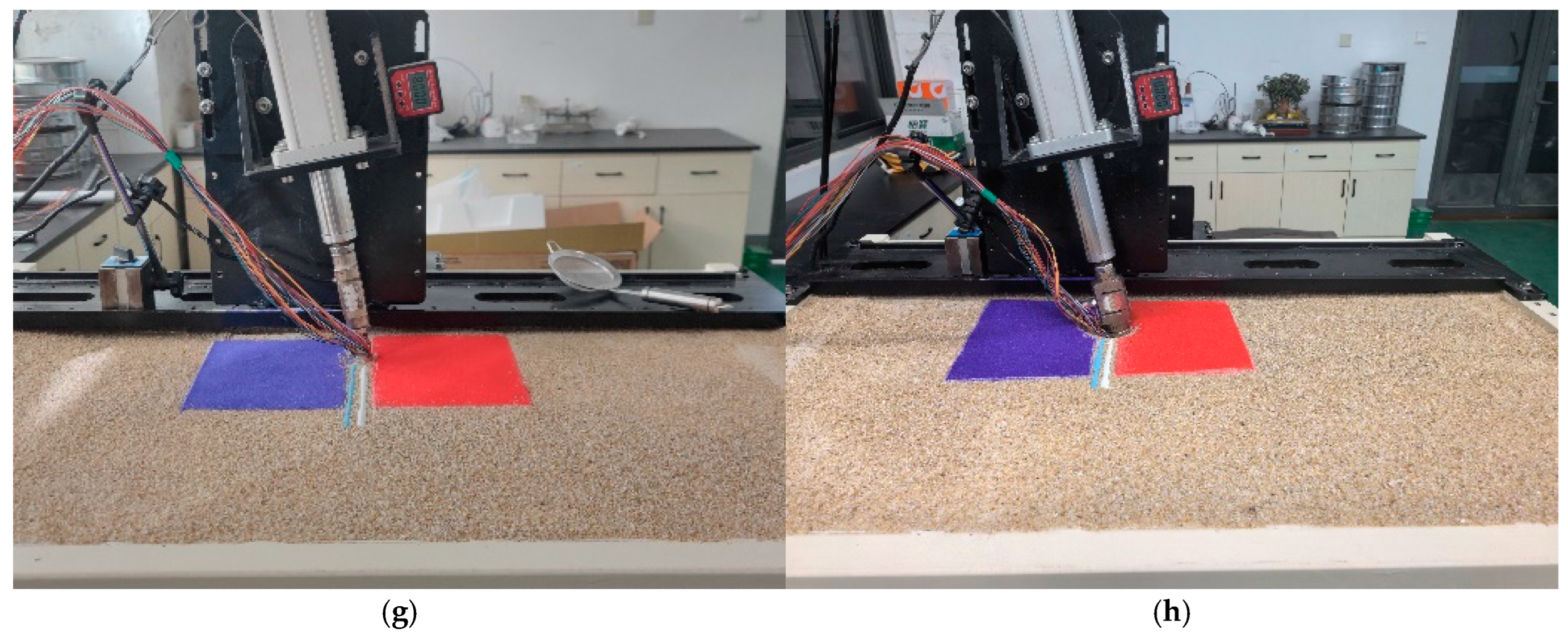
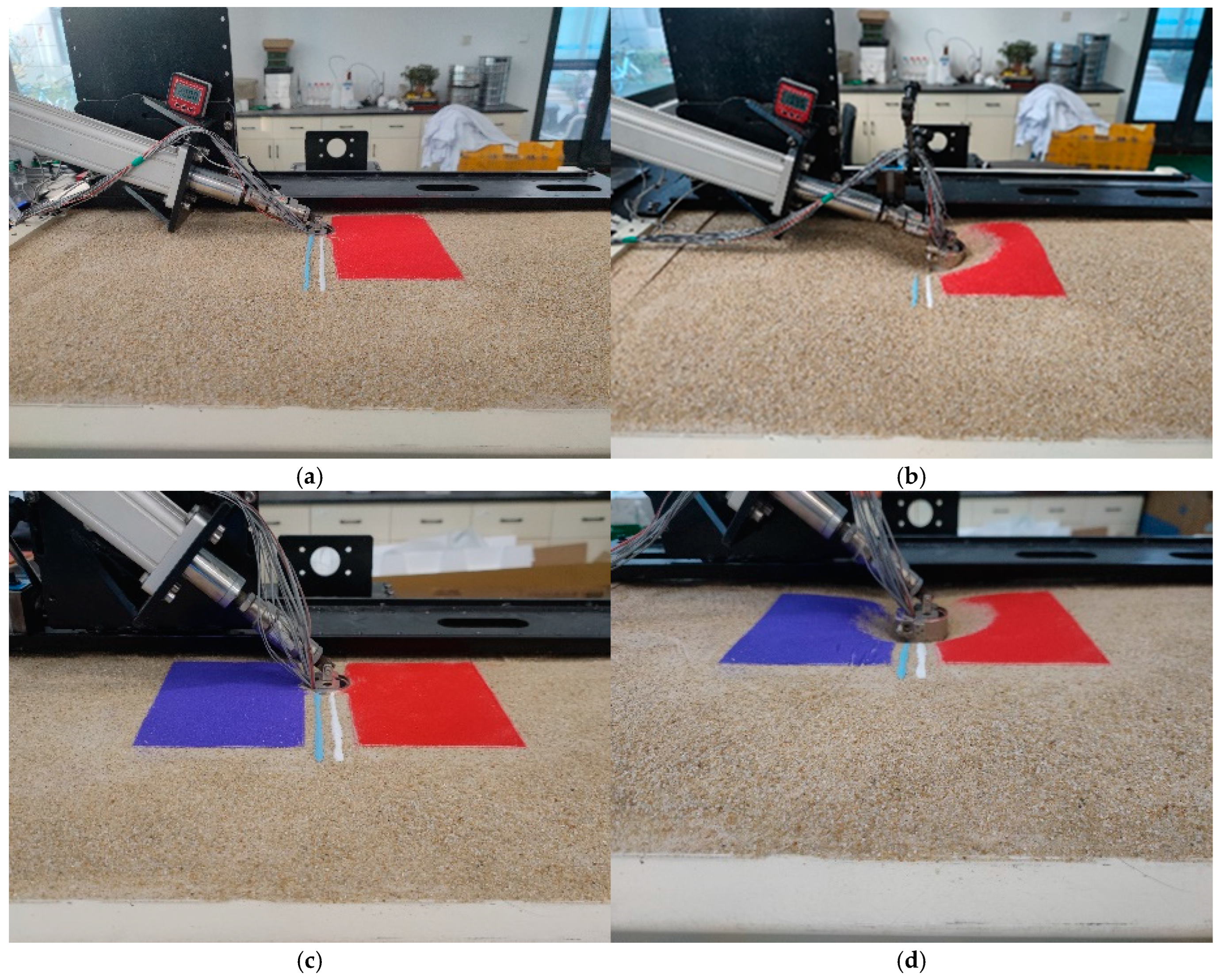
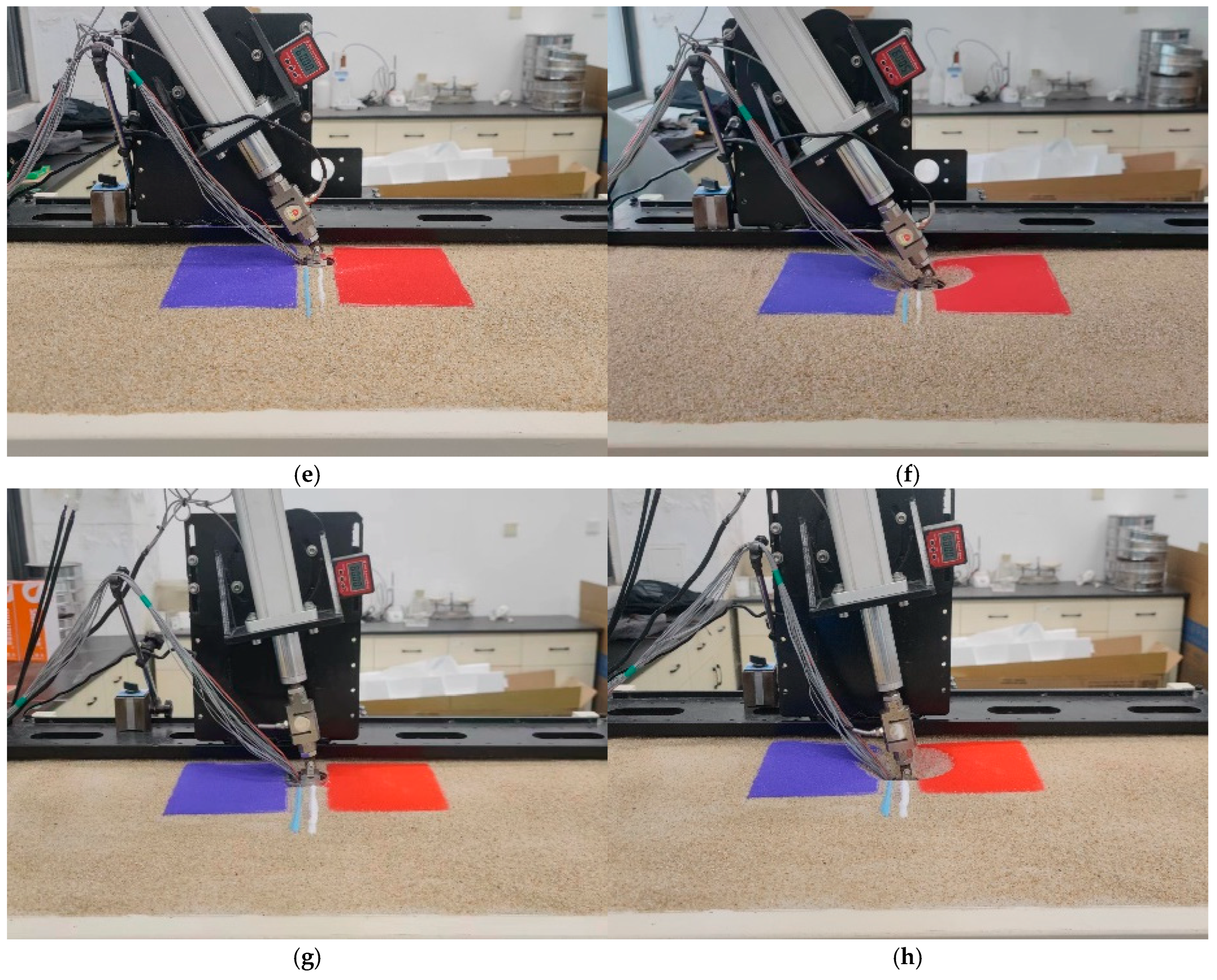
2.1. Cyclic Loading System

As shown in Figure 1, the test model box measures 1 m (length) × 0.7 m (width) × 1 m (height), meeting the boundary conditions. A steel frame capable of 180° free rotation is installed on top of the model box. The loading device features a high-stroke, high-load servo cylinder system with a maximum displacement stroke of 30 cm and a maximum push/pull force of 6 kN, enabling continuous, uninterrupted, and cyclic loading. Additionally, the equipment includes a displacement sensor, a displacement acquisition system, and other components.

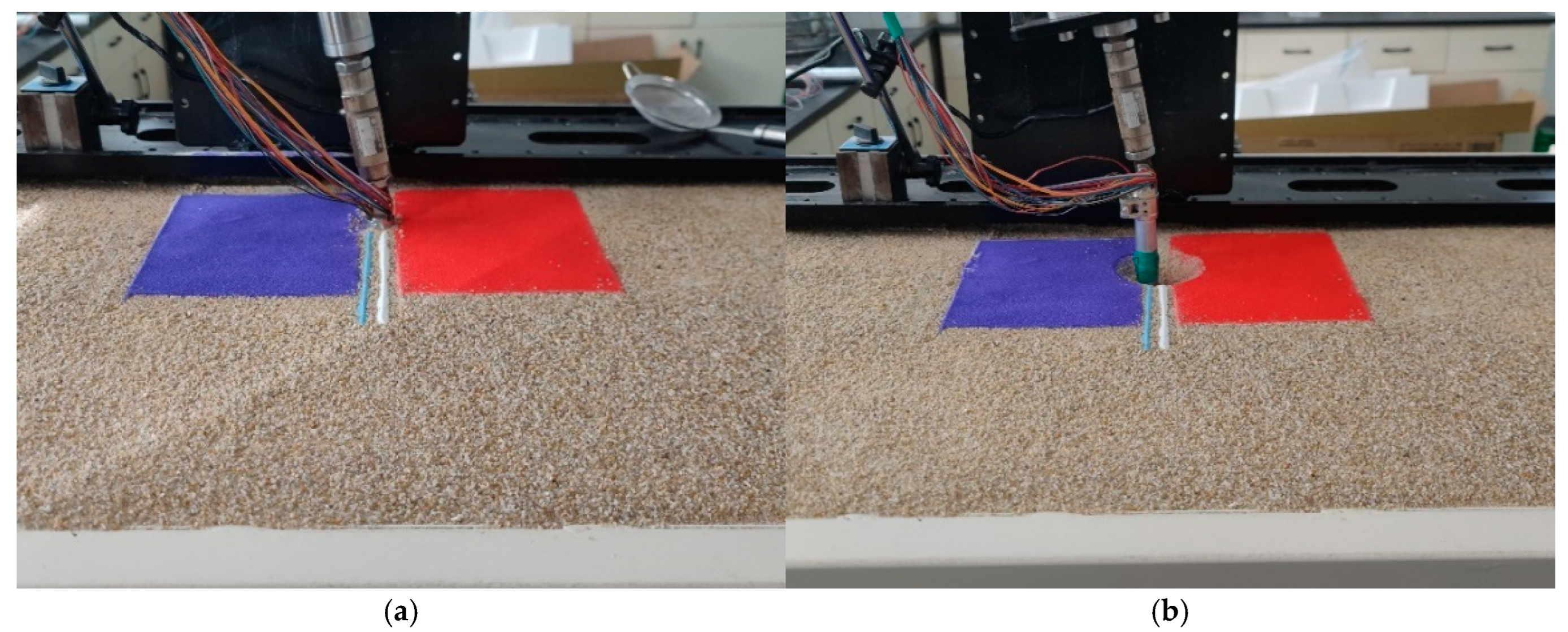
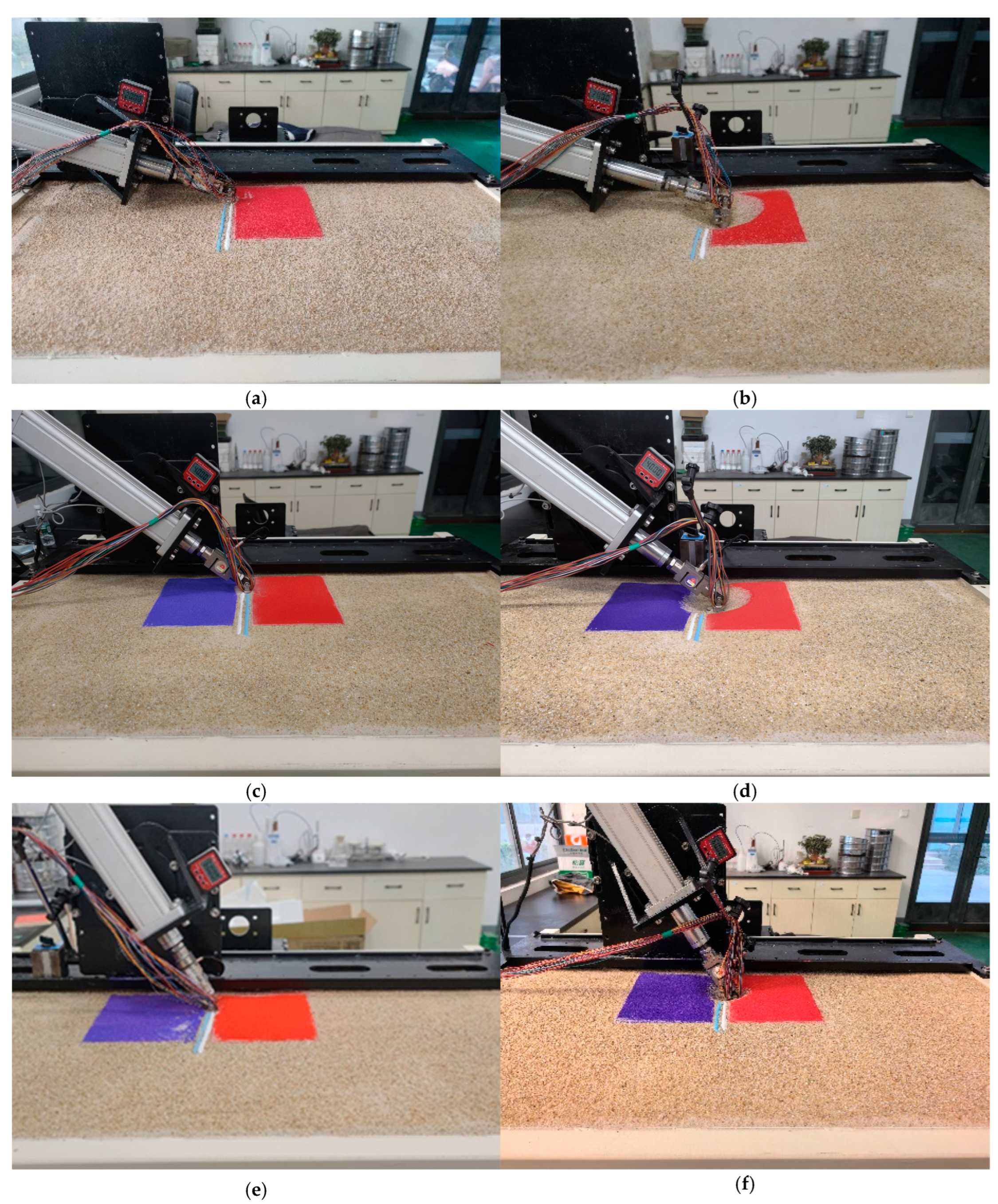
2.2. Test the Preparation of Soil Samples

Fujian standard sand was used as the foundation soil for this experiment, and its grading curve is shown in Figure 2. Layer compaction every 10 cm thickness, followed by tamping and smoothing treatment to enhance bonding strength. During the compaction process, the density of the sand was measured three times, with an average value of approximately 1.77 g/cm³ and a variation within 5%, yielding an average relative density D_r of around 62%. The mechanical properties of the sandy soil are shown in

Table 1. Physical characteristics of soil.

Soil Characteristics	Parameter Values
The average particle size D50 (mm)	0.17
Maximum dry weight ρmin (kN/m3)	1.978
Minimum dry weight ρmax (kN/m3)	1.495
Moisture content	2%
Specific gravity of soil particles Gs	2.632
Relative density Dr	62%

.

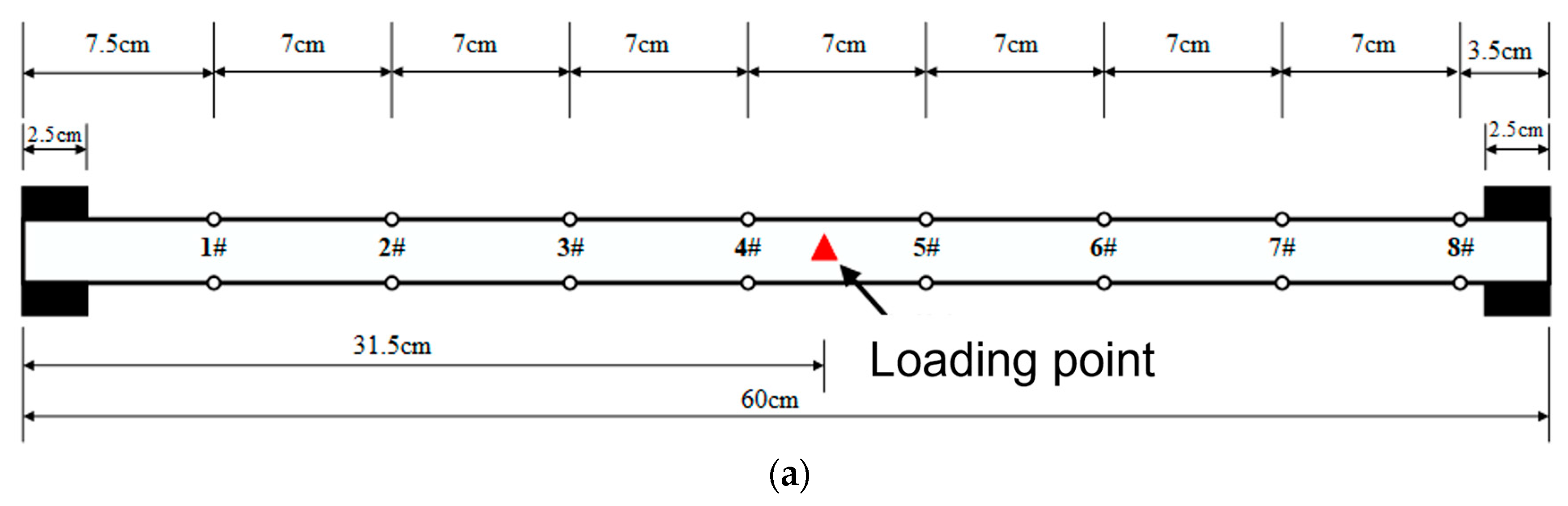
2.3. Design and Manufacture of Pile Specimen

As shown in Figure 3, thin-walled hollow aluminum alloy tubes were used to construct the model piles. Strain gauges were installed at 7 cm intervals on both sides in a symmetrical arrangement to capture strain data throughout the experiment. To prevent damage to the strain gauges, holes were drilled 1.5 cm above each gauge, through which the wiring was passed into the pile and routed to the top. This experiment used the simple beam theory method for calibration, and the elastic moduli of A and B piles were 72.89 GPa and 67.47 GPa. Two model piles, A and B, were made in this experiment, and detailed parameters were shown in

Table 2. Material parameters of pile.

ID	Length L (cm)	Diameter D (cm)	Pile Wall Thickness T (cm)	T/L
A	60	2	0.1	0.190
B	60	5	0.2	0.375

.

The pile–soil relative stiffness coefficient was calculated using the following Reese method [24,25]:

$$\left\{\begin{array}{l}{\displaystyle \frac{T}{L}}<0.2\mathrm{Flexible}\mathrm{pile}\\ {\displaystyle \frac{T}{L}}>0.5\mathrm{Rigid}\mathrm{pile}\end{array}\right.,T=\sqrt[5]{{\displaystyle \frac{E_{\mathrm{p}}{I}_{\mathrm{p}}}{n_h}}}$$

(1)

where T/L is the pile–soil relative stiffness; E_pI_p is the pile’s flexural stiffness; and n_h is the foundation reaction modulus (n_h in this paper is 10.2 MN/m³, based on the recommended value from the U.S. ACE manual (Figure 4)).

2.4. Test Scheme

In this test, all cyclic numbers (N) were 10,000, and the loading was applied unidirectionally. The inclined angle (θ_L), formed between the direction of the load and the horizontal line, was set at various inclined angles: 0°, 20°, 40°, 60°, and 80°. The selection range for cyclic amplitude ratio (ζ_b) is from 0.3 to 0.7, and for cyclic load ratio (ζ_c) it is from 0 to 0.6 [13]. The groupings of the tests are provided in

Table 3. Groupings of model tests.

ID	Load Type	Cyclic Amplitude Ratio (ζb)	Cyclic Load Ratio (ζc)	Cycle Number (N)
A-1	0°	0.5	0.2	10,000
A-2	20°	0.5	0.2	10,000
A-3	40°	0.5	0.2	10,000
A-4	60°	0.5	0.2	10,000
A-5	80°	0.5	0.2	10,000
B-1	0°	0.5	0.2	10,000
B-2	20°	0.5	0.2	10,000
B-3	40°	0.5	0.2	10,000
B-4	60°	0.5	0.2	10,000
B-5	80°	0.5	0.2	10,000

.

In the initial test conditions, a fully unidirectional cyclic loading was assumed (that is, ζ_c = 0). However, it was found that due to the feedback lag of the PID controller, when the load was unloaded close to 0, the electric cylinder continued to slowly retract but never fully reset to 0. This caused the pile to be slightly pulled out of the soil layer with each cycle. After several cycles, the pile would be significantly lifted out of the soil (as shown in Figure 5). Through multiple loading tests, it was found that setting the minimum value of ζ_c around 0.15 could prevent this phenomenon. In this experiment, ζ_c was set to 0.2.

3. Cumulative Deformation Test Results and Analysis

To observe the subsidence of surrounding soil under inclined cyclic loading, a layer of colored sand was spread on the ground and in the opposite direction of the cyclic load before each test. Additionally, 1–2 colored sand lines were placed on the side. Figure 6 and Figure 7 show the comparison images of piles A and B before and after the tests, respectively.

As shown in Figure 6 and Figure 7, it can be observed that when ζ_b, ζ_c, and T/L are kept constant, the greater θ_L, the smaller the radius of the subsidence, and the shallower the depth of the surrounding sandy soil after 10,000 cycles. For instance, in the B-2 (θ_L = 20°) test, the maximum subsidence from the initial pile position was 13.5 cm, with a depth of 5 cm. In contrast, for the B-5 (θ_L = 80°) test, the maximum subsidence was only 8 cm away from the initial pile position, with a depth of 3.5 cm. The reason for this is that as θ_L increases, while the load magnitude remains constant, the horizontal component decreases, leading to reduced subsidence of the surrounding soil.

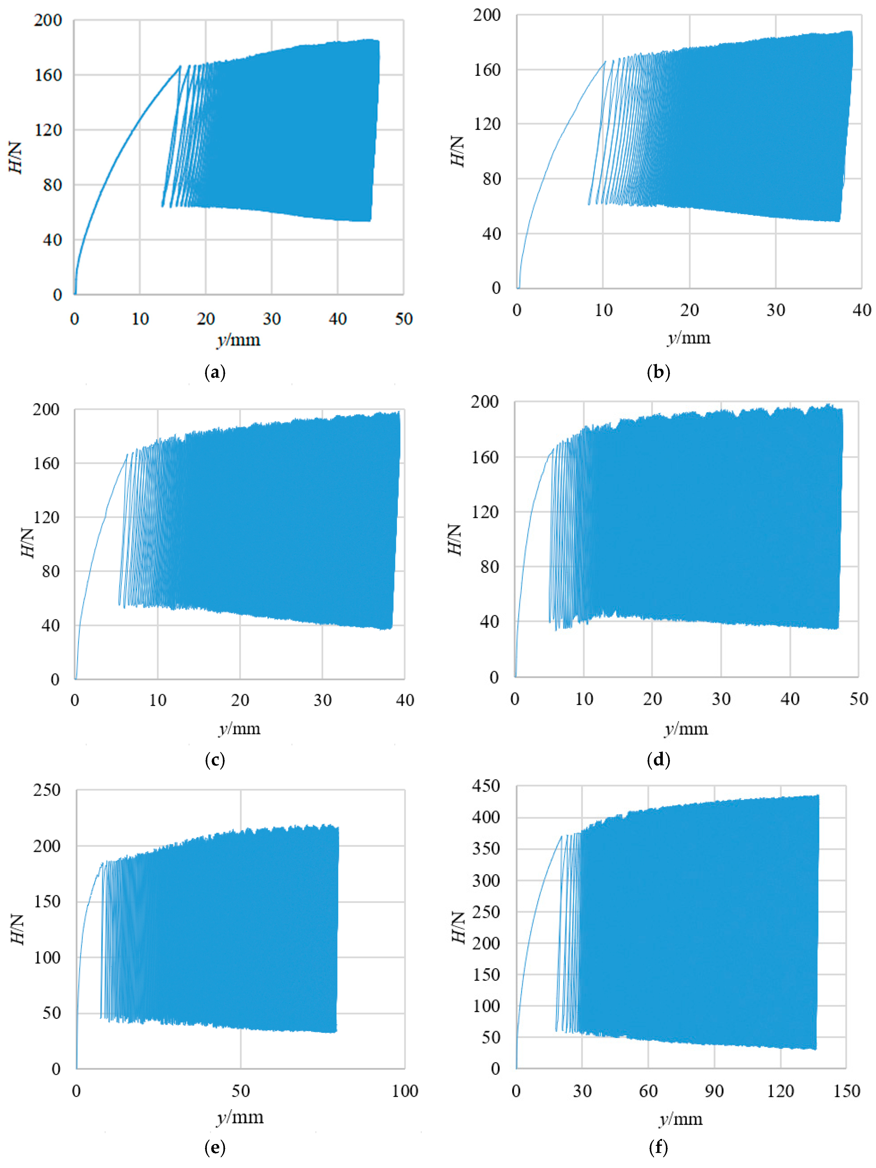
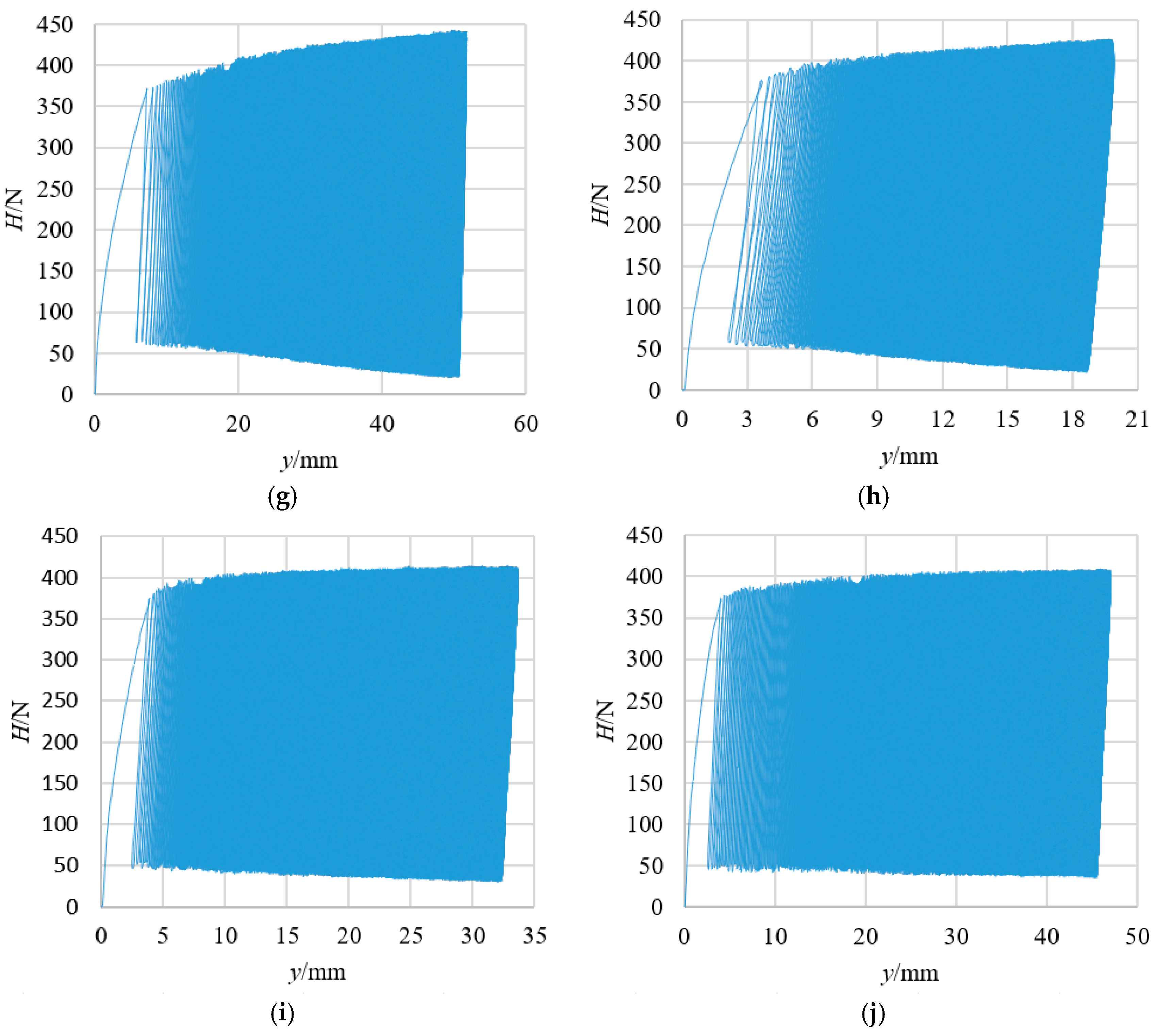
3.1. Load–Displacement Curve Under Inclined Cyclic Load

The Q-s curve of piles A and B inclined cyclic loading test is shown in Figure 8. The hysteresis curves exhibit distinct hysteresis characteristics, with the hysteresis loops gradually shifting to the right as N increases, and the cumulative displacement keeps developing. In the initial stages, displacement accumulation is rapid, hysteresis loops are large, and exhibit minimal overlap. As N increases, the surrounding sandy soil becomes denser due to subsidence, leading to smaller and more overlapping hysteresis loops, with slower displacement accumulation. This is consistent with the results of model tests on horizontal cyclic loading conducted by Wang Yang [17], Cuéllar et al. [26], Abadie et al. [27], and others.

Comparing Figure 8f–j, as θ_L increases from 0° to 80°, the peak displacement at the pile top under initial loading decreases from approximately 18 mm in the B-1 test to about 3 mm in the B-5 test. This is due to the combined horizontal and vertical displacements under inclined cyclic loading, where increased vertical load reduces overall displacement. However, the final cumulative displacement after cycling decreases from 140 mm in the B-1 test to 20 mm in the B-3 test and then increases to 47 mm in the B-5 test. This indicates that as θ_L increases, the final cumulative displacement after 10,000 cycles first decreases and then increases.

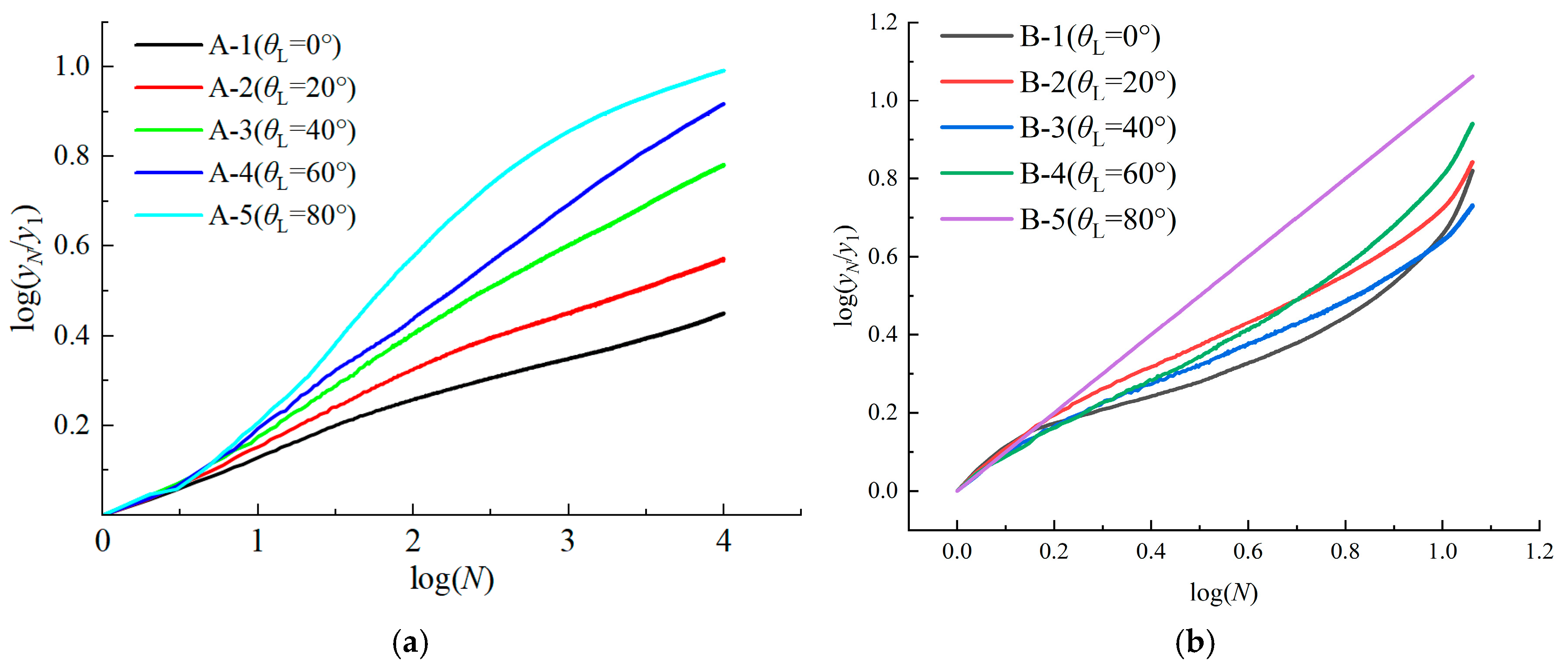
3.2. Development Law of Cumulative Displacement

To further investigate the progression trend of cumulative displacement at the top of the pile under inclined cyclic loading, this study employed the ratio method to process the data, where the ratio of the peak displacement at the Nth cycle (y_N) to the peak displacement at the initial cycle (y₁) was used as the normalized cumulative displacement (y_N/y₁). The relationship curve between y_N/y₁ and N is illustrated in Figure 9.

The results show that y_N/y₁ increases as N rises. At the initial stage of loading, the growth rate of y_N/y₁ is rapid, but as N continues to increase, the growth rate gradually slows down. Additionally, when ζ_b, ζ_c, and T/L remain constant, a larger θ_L leads to a faster accumulation rate of cyclic displacement.

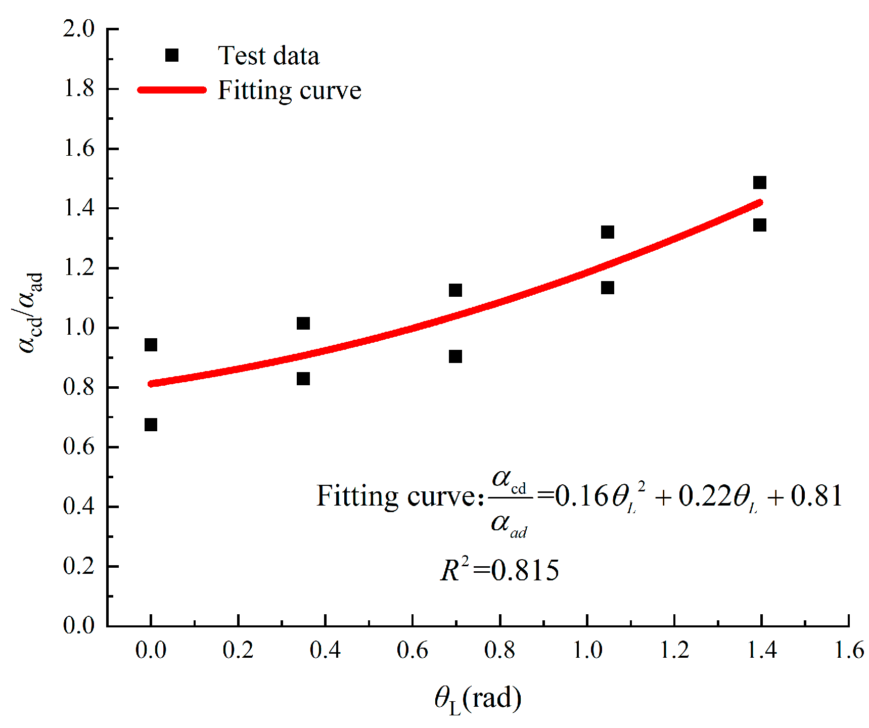
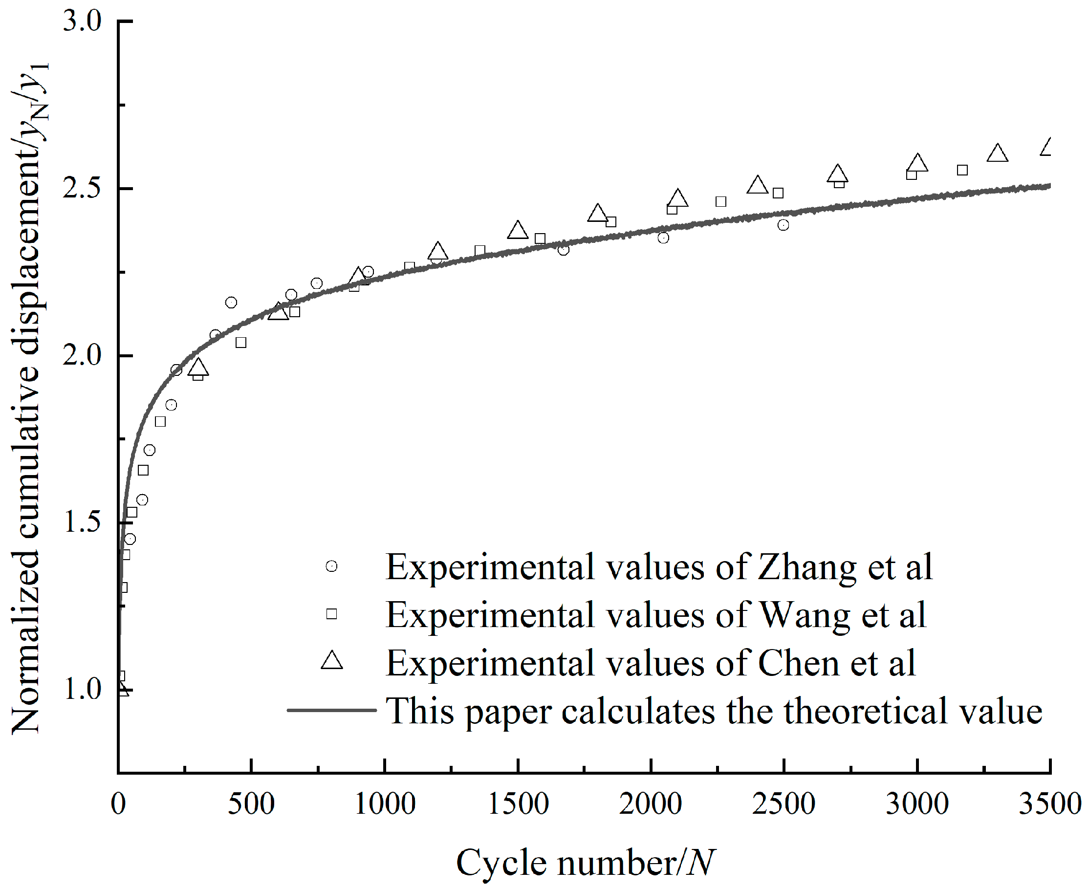
3.3. Prediction Formula of Cumulative Displacement

The relationship between y_N/y₁ and N for each test group in Figure 10 was processed using a double logarithmic scale, as shown in Figure 10. The log–log plot of y_N/y₁ versus N reveals an approximately clear proportional relationship.

The relationship between y_N/y₁ and N can be expressed as Equation (2).

$$\log \left({\displaystyle \frac{y_N}{y_1}}\right)={\alpha }_{cd}\log (N)$$

(2)

where y₁ represents the first period peak displacement, y_N represents the Nth period peak displacement corresponding, and α_cd is the cumulative displacement coefficient for inclined cyclic loading.

The cumulative displacement prediction formula for piles under inclined cyclic loading studied in this paper is derived through further research based on the prediction formula of cumulative displacement for piles under lateral cyclic loading (Equation (3)) proposed by Chen et al. [21].

$${\alpha }_{ad}=f\left({\displaystyle \raisebox{1ex}{$T$}\!\left/ \!\raisebox{-1ex}{$L$}\right.}\right)g\left({\zeta }_c\right)=\left(0.22\times {\displaystyle \frac{T}{L}}+0.16\right)\left(-0.7{\zeta }_c+1\right)$$

(3)

Therefore, let:

$${\alpha }_{cd}=p\left({\theta }_{\mathrm{L}}\right){\alpha }_{ad}$$

(4)

where p(θ_L) represents the influence coefficient of θ_L; α_ad is the cumulative displacement coefficient for piles under horizontal cyclic loading, determined by Equation (3).

The expression p(θ_L) can be derived as follows:

$$p\left({\theta }_{\mathrm{L}}\right)={\displaystyle \frac{{\alpha }_{cd}}{{\alpha }_{ad}}}$$

(5)

The statistical results of the inclined cyclic loading test data are shown in

Table 4. Summary of parameters for inclined cyclic test.

ID	ζc	T/L	θL (rad)	αad	αcd	αcd/αad
A-1	0.2	0.190	0	0.145	0.118	0.814
A-2	0.2	0.190	0.349	0.145	0.145	1
A-3	0.2	0.190	0.698	0.145	0.197	1.359
A-4	0.2	0.190	1.047	0.145	0.231	1.593
A-5	0.2	0.190	1.396	0.145	0.260	1.793
B-1	0.2	0.375	0	0.209	0.197	0.943
B-2	0.2	0.375	0.349	0.209	0.212	1.014
B-3	0.2	0.375	0.698	0.209	0.189	0.904
B-4	0.2	0.375	1.047	0.209	0.237	1.134
B-5	0.2	0.375	1.396	0.209	0.281	1.344

. For the convenience of fitting the following equations, θ_L has been converted to radians. The relationship curve between θ_L and p(θ_L) is plotted as shown in Figure 11.

From Figure 11, it can be observed that p(θ_L) exhibits a significant correlation with θ_L. By applying a quadratic fitting approach to the data, the expression for p(θ_L) is obtained as follows:

$$p\left({\theta }_{\mathrm{L}}\right)={\displaystyle \frac{{\alpha }_{cd}}{{\alpha }_{ad}}}=0.16{\theta }_L^2+0.22{\theta }_L+0.81$$

(6)

By combining Equations (3), (4), and (6), the final expression for α_cd can be derived as follows:

$${\alpha }_{cd}=\left(0.16{\theta }_L^2+0.22{\theta }_L+0.81\right)\left(0.22\times {\displaystyle \frac{T}{L}}+0.16\right)\left(-0.7{\zeta }_c+1\right)$$

(7)

Equation (7) is substituted into Equation (2) to derive the following normalized fitting prediction formula for inclined cyclic cumulative displacement:

$$\log \left({\displaystyle \frac{y_N}{y_1}}\right)=\left(0.16{\theta }_L^2+0.22{\theta }_L+0.81\right)\left(0.22\times {\displaystyle \frac{T}{L}}+0.16\right)\left(-0.7{\zeta }_c+1\right)\log (N)$$

(8)

To verify the reliability of the predictive Equation (8), the inclination inclined angle is set to 0 and compared with the horizontal cyclic predictive formulas of other scholars, as shown in Figure 12. It can be seen that the prediction model in this study has good reliability [28].

At present, there is a lack of studies on cyclic loading considering inclination in the inclined angle. To further verify the validity of Equation (8), several representative numbers of cycles were selected. Using Equation (8), the experimental parameters in Table 4 were calculated to obtain the k_lN/k_l1 values for each group, which were then compared with the actual test data of k_lN/k_l1. The results are shown in

Table 5. Summary table of Equation (8).

A-2	N	Test Data yN	Equation (19) yN	Error Rate (%)	A-3	N	Test Data yN	Equation (19) yN	Error Rate (%)
	1000	29.03	30.38	4.65		1000	25.52	22.24	12.85
	2000	31.39	33.88	7.93		2000	28.87	25.21	12.68
	5000	35.03	39.13	11.7		5000	34.22	29.75	13.06
	10,000	38.23	43.64	14.15		10,000	38.52	33.72	12.46
B-2	N	Test Data yN	Equation (19) yN	Error Rate (%)	B-4	N	Test Data yN	Equation (19) yN	Error Rate (%)
	1000	32.44	26.97	−16.86		1000	19.63	22.19	13.04
	2000	37.24	30.75	−17.43		2000	23.51	26.45	12.51
	5000	44.49	36.56	−17.82		5000	29.15	33.37	14.48
	10,000	50.84	41.68	−18.02		10,000	33.5	39.78	18.75

.

As shown in Table 5, all errors are below 20%, confirming the validity of the normalized fitting prediction formula for inclined cyclic cumulative displacement developed in this study.

4. Loading and Unloading Stiffness Test Results and Analysis

To further investigate the characteristics of stiffness variation during cyclic loading and cyclic unloading, this study defines the cyclic loading stiffness under the Nth cyclic as k_lN and the corresponding cyclic unloading stiffness as k_uN.

$$k_{lN}={\displaystyle \frac{H_{\max }-H_{\min }}{y_N-y_{rN}}}$$

(9)

$$k_{uN}={\displaystyle \frac{H_{\max }-H_{\min }}{y_{\left(N-1\right)}-y_{rN}}}$$

(10)

where y_N and y_rN represent the peak displacement and residual displacement, respectively, during the Nth cyclic loading. The definitions of these two types of stiffness are illustrated in Figure 13.

Some scholars have used the secant stiffness method, connecting the cyclic peak displacement with the origin, to study the cyclic stiffness of pile foundations [29]. Although this method can show the cumulative displacement under cyclic loading, it only provides conclusions related to stiffness degradation.

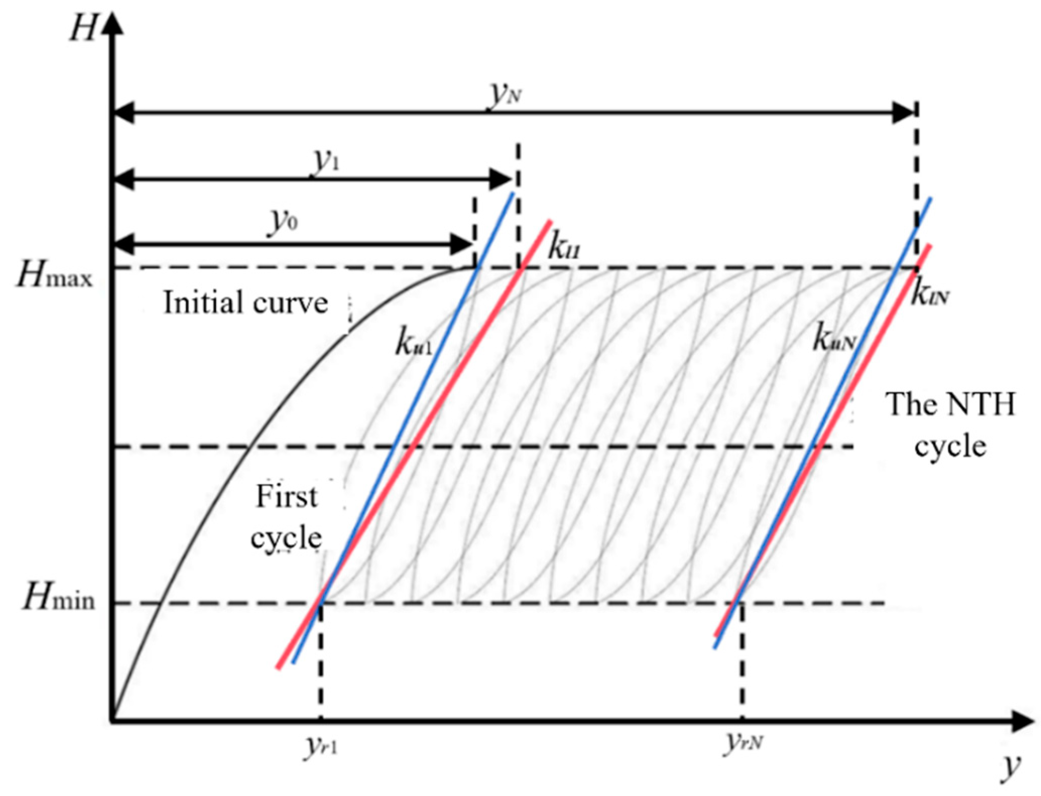
4.1. Development Law of Inclined Cyclic Loading Stiffness

According to Equation (9), the load–displacement curve data are processed to obtain the k_lN value, which is then normalized by dividing k_lN by k_l1 (the initial cycle loading stiffness). Figure 14 shows the relationship of the normalized cyclic loading stiffness (k_lN/k_l1) varying with N.

The results indicate that in the early stages of cyclic loading, the reconstitution and densification of the surrounding sand soil around the pile cause the cyclic loading stiffness to increase rapidly. The larger the θ_L, the steeper the increase. When N approaches 1000, the curve shows a turning point, as the cyclic densification process of the surrounding sand soil leads to a gradual slowdown in the growth rate. Furthermore, the larger the θ_L, the quicker the transition from rapid growth to a stable state of stiffness. When θ_L reaches 80° (as shown in Figure 14e,j), the k_lN/k_l1 value peaks at the beginning and remains almost unchanged thereafter.

A comparison of Figure 14a–e reveals that, under the same 10,000 loading cycles, as θ_L increases, the k_lN/k_l1 value of pile A initially decreases and then increases (the ratio decreases from 3.7 to 2.2 as θ_L increases from 0° to 60°, but then increases to 3.2 as θ_L further increases to 80°). However, comparing Figure 14f–g, it is found that, as θ_L increases, the k_lN/k_l1 value of pile B gradually decreases (the ratio decreases from 5.5 to 1.62 as θ_L increases from 0° to 80°). The difference in the stiffness change behavior between model piles A and B may be related to the relative stiffness of the pile–soil system, which will be further investigated.

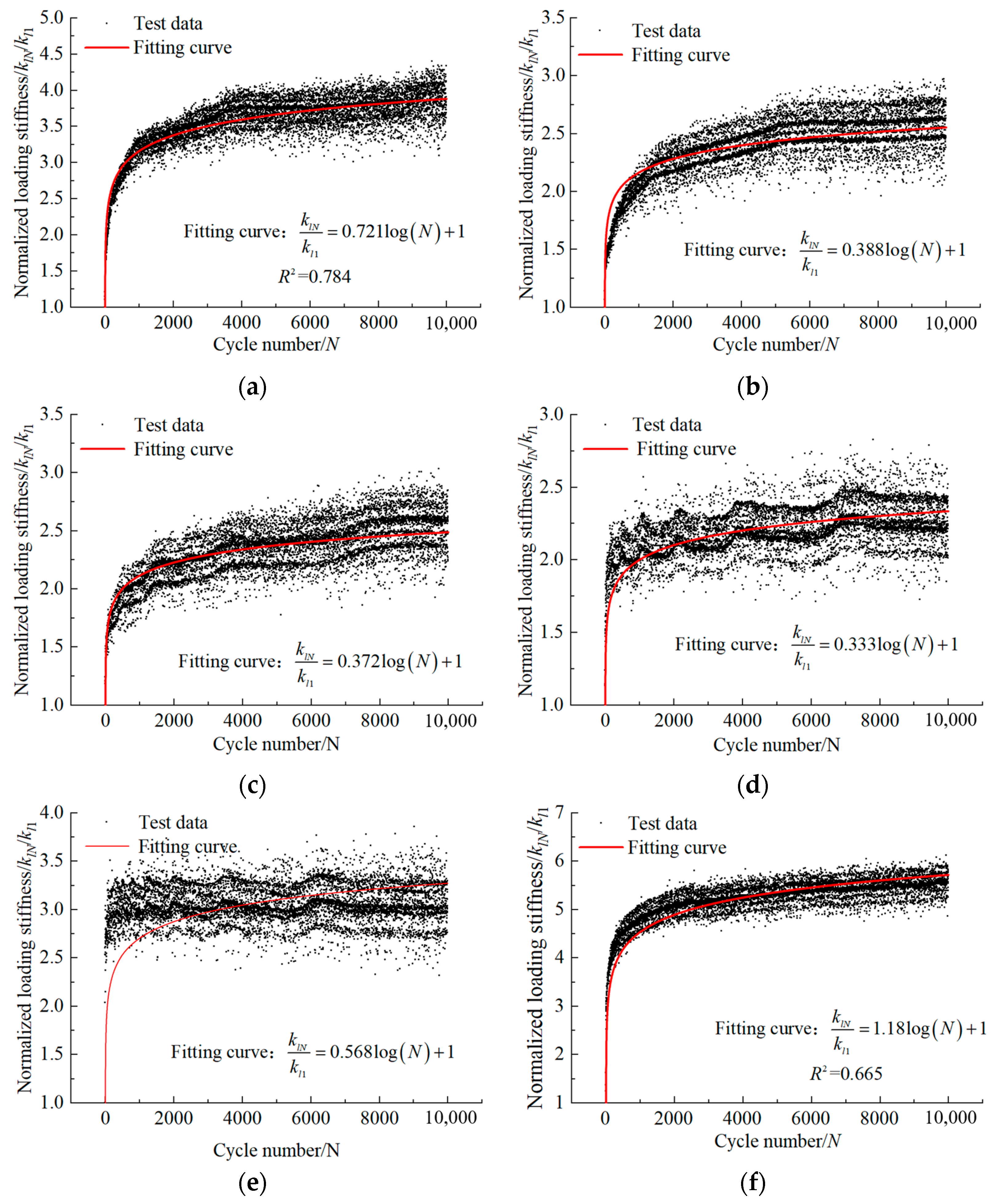
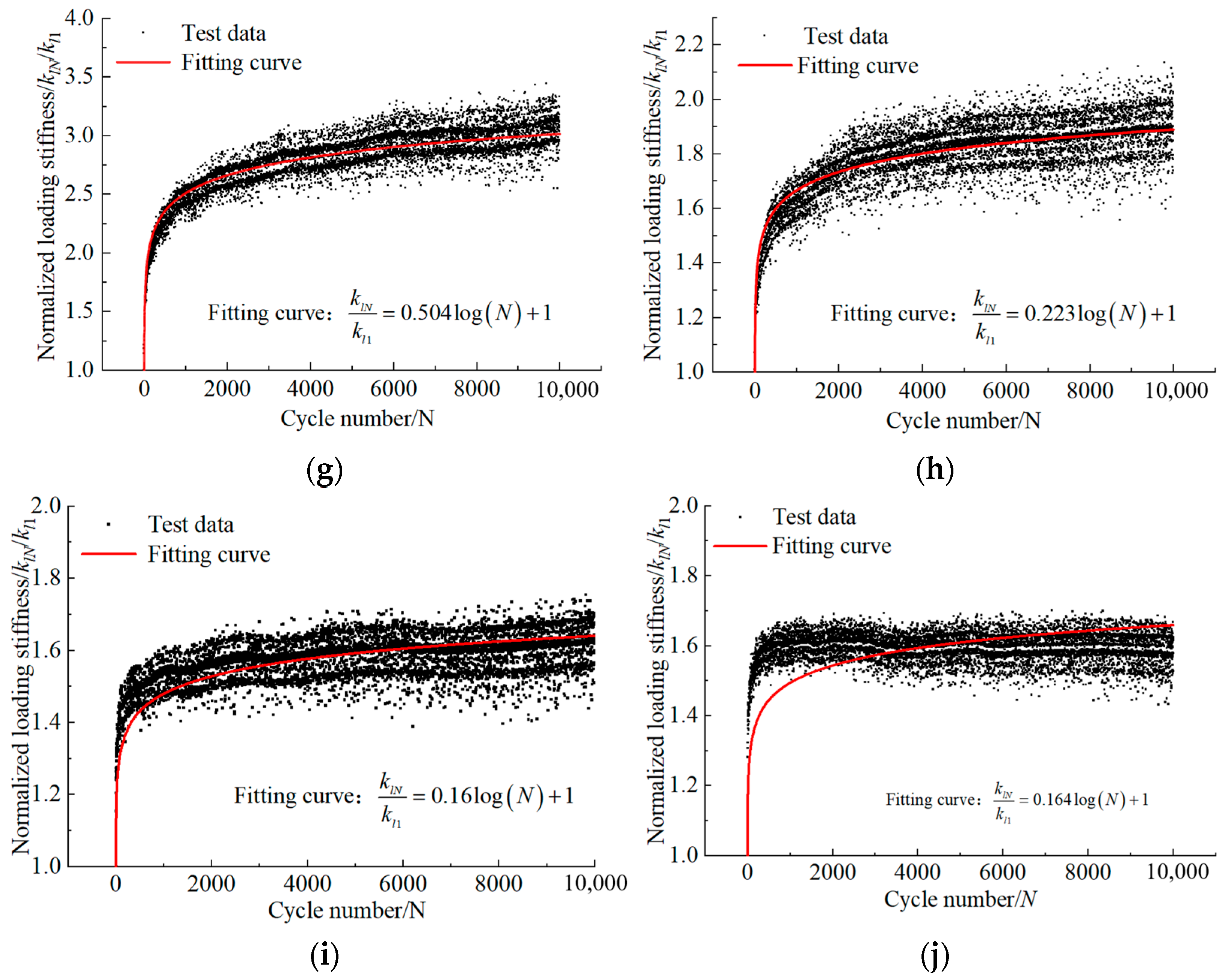
4.2. Prediction Formula of Inclined Cyclic Loading Stiffness

This study on the variation of pile stiffness under inclined cyclic loading builds upon the results of horizontal cyclic loading studies by Chen et al. [21], as presented in Equation (11).

$${\beta }_l=\left[1.34\left({\displaystyle \frac{T}{L}}\right)+0.38\right]\left(-6.27{\zeta }_c^2+2.33{\zeta }_c+1.02\right)\left(-2.49{\zeta }_b^2+2.91{\zeta }_b+0.16\right)$$

(11)

As shown in Figure 15, the ratio k_lN/k_l1 exhibits a logarithmic relationship with N. Additionally, considering that k_lN/k_l1 equals 1 when N equals 1, the following expression for the inclined cyclic loading stiffness can be established:

$${\displaystyle \frac{k_{lN}}{k_{l1}}}={\beta }_L\log \left(N\right)+1$$

(12)

where k_l1 represents the stiffness during the first inclined cyclic loading; k_lN represents the stiffness during the Nth inclined cyclic loading; and β_L is the inclined cyclic loading stiffness coefficient. Let:

$${\beta }_L=p_1\left({\theta }_{\mathrm{L}}\right){\beta }_l$$

(13)

where p₁(θ_L) is the coefficient representing the effect of the θ_L on the inclined cyclic loading stiffness of the pile, and β_l is the horizontal cyclic loading stiffness coefficient.

The expression for p₁(θ_L) can be derived as follows:

$$p_1\left({\theta }_{\mathrm{L}}\right)={\displaystyle \frac{{\beta }_L}{{\beta }_l}}$$

(14)

The summary of the fitting curve results of the relationship between k_lN/k_l1 and N in Figure 15 is shown in

Table 6. Summary of k_lN/k_l1 fitting expressions.

ID	ζb	ζc	T/L	θL (rad)	βl	Fitting Formula	βL	βL/βl
A-1	0.5	0.2	0.190	0	0.778	${\displaystyle \frac{k_{lN}}{k_{l1}}}=0.721\log \left(N\right)+1$	0.721	0.927
A-2	0.5	0.2	0.190	0.349	0.778	${\displaystyle \frac{k_{lN}}{k_{l1}}}=0.388\log \left(N\right)+1$	0.388	0.499
A-3	0.5	0.2	0.190	0.698	0.778	${\displaystyle \frac{k_{lN}}{k_{l1}}}=0.372\log \left(N\right)+1$	0.372	0.478
A-4	0.5	0.2	0.190	1.047	0.778	${\displaystyle \frac{k_{lN}}{k_{l1}}}=0.333\log \left(N\right)+1$	0.333	0.428
A-5	0.5	0.2	0.190	1.396	0.778	${\displaystyle \frac{k_{lN}}{k_{l1}}}=0.568\log \left(N\right)+1$	0.568	0.730
B-1	0.5	0.2	0.375	0	1.08	${\displaystyle \frac{k_{lN}}{k_{l1}}}=1.18\log \left(N\right)+1$	1.181	1.092
B-2	0.5	0.2	0.375	0.349	1.08	${\displaystyle \frac{k_{lN}}{k_{l1}}}=0.504\log \left(N\right)+1$	0.504	0.466
B-3	0.5	0.2	0.375	0.698	1.08	${\displaystyle \frac{k_{lN}}{k_{l1}}}=0.223\log \left(N\right)+1$	0.223	0.206
B-4	0.5	0.2	0.375	1.047	1.08	${\displaystyle \frac{k_{lN}}{k_{l1}}}=0.16\log \left(N\right)+1$	0.16	0.148
B-5	0.5	0.2	0.375	1.396	1.08	${\displaystyle \frac{k_{lN}}{k_{l1}}}=0.164\log \left(N\right)+1$	0.165	0.152

, and the relationship between p₁(θ_L) and θ_L is drawn as shown in Figure 16.

Figure 15 shows that the k_lN/k_l1 of piles A and B varies inconsistently with θ_L, and the two sets of data cannot be fitted together. The fitting results from Chen et al. [21] primarily focus on semi-rigid piles. This study distinguishes the differences in the variation of cyclic loading stiffness with θ_L between semi-rigid piles and slender piles:

(1) The functional expression for slender piles is as follows:

$${\displaystyle \frac{{\beta }_L}{{\beta }_l}}=0.84{\theta }_L^2-1.3{\theta }_L+0.91$$

(15)

Combining Equations (11), (13), and (15), the cyclic loading stiffness coefficient β_Lf for flexible piles under inclined cyclic loading is obtained as follows:

$${\beta }_{\mathrm{Lf}}=\left[1.34\left({\displaystyle \frac{T}{L}}\right)+0.38\right]\left(-6.27{\zeta }_c^2+2.33{\zeta }_c+1.02\right)\left(-2.49{\zeta }_b^2+2.91{\zeta }_b+0.16\right)\left(0.84{\theta }_L^2-1.3{\theta }_L+0.91\right)$$

(16)

(2) The functional expression for semi-rigid piles is as follows:

$${\displaystyle \frac{{\beta }_L}{{\beta }_l}}=0.86{\theta }_L^2-1.82{\theta }_L+1.06$$

(17)

Combining Equations (11), (13), and (17), the cyclic loading stiffness coefficient β_Ls for flexible piles under inclined cyclic loading is obtained as follows:

$${\beta }_{\mathrm{Ls}}=\left[1.34\left({\displaystyle \frac{T}{L}}\right)+0.38\right]\left(-6.27{\zeta }_c^2+2.33{\zeta }_c+1.02\right)\left(-2.49{\zeta }_b^2+2.91{\zeta }_b+0.16\right)\left(0.86{\theta }_L^2-1.82{\theta }_L+1.06\right)$$

(18)

By substituting Equations (16) and (18) into Equation (12), the following prediction formula of the inclined cyclic loading stiffness is derived:

$$\begin{array}{l}{\displaystyle \frac{k_{lN}}{k_{l1}}}=\left\{\begin{array}{l}{\beta }_l\left(0.84{\theta }_L^2-1.3{\theta }_L+0.91\right)\log \left(N\right)+1\mathrm{Slender}\mathrm{pile}\\ {\beta }_l\left(0.86{\theta }_L^2-1.82{\theta }_L+1.06\right)\log \left(N\right)+1\mathrm{Semi-rigid}\mathrm{pile}\end{array}\right.,\\ \mathrm{Where},{\beta }_l=\left[1.34\left({\displaystyle \frac{T}{L}}\right)+0.38\right]\left(-6.27{\zeta }_c^2+2.33{\zeta }_c+1.02\right)\left(-2.49{\zeta }_b^2+2.91{\zeta }_b+0.16\right)\end{array}$$

(19)

To verify the validity of Equation (19), several representative numbers of cycles were selected. Using Equation (19), the experimental parameters in Table 6 were calculated to obtain the k_lN/k_l1 values for each group, which were then compared with the actual test data of k_lN/k_l. The results are presented in Table 8 in Section 4.4 of this paper.

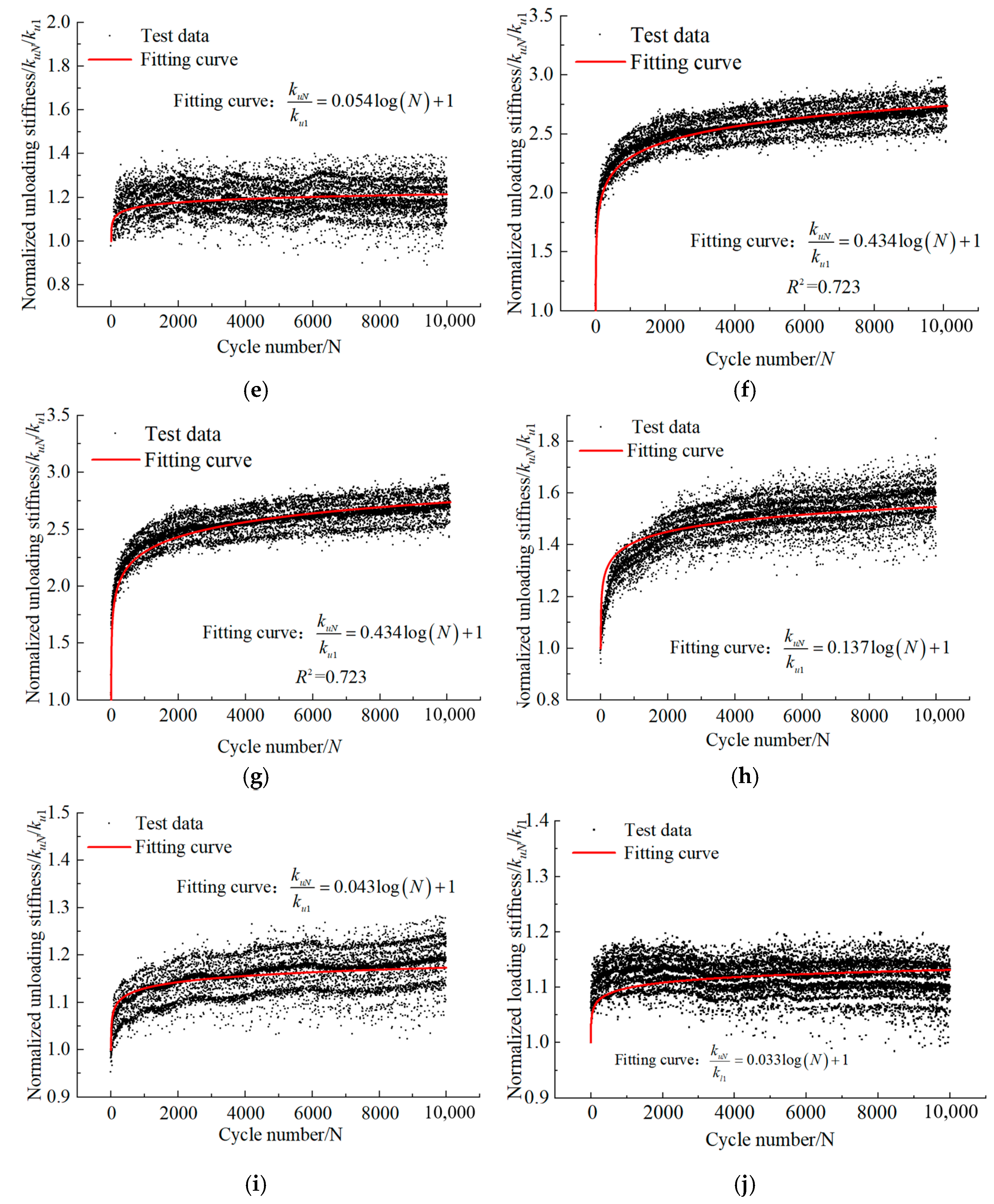
4.3. Development Law of Inclined Cyclic Unloading Stiffness

Similar to the research method for loading stiffness, the Q-s curve data are processed using Equation (10) determine the k_uN value, which is then normalized by dividing k_uN by k_u1(the initial cycle unloading stiffness). Figure 16 shows the relationship of the normalized cyclic unloading stiffness (k_uN/k_u1) varying with N.

As shown in Figure 16, the cyclic unloading stiffness increases with the increase in N, following the same pattern as the cyclic loading stiffness. Specifically, in group A-5 (θ_L = 80°), the k_uN/k_u1 values also exhibit a trend slightly higher than those in group A-4 (θ_L = 60°). Further, as shown in Figure 16a–e, the overall k_uN/k_u1 values of group Al-1 (θ_L = 0°) are higher than those of group A-5 (θ_L = 80°). A similar conclusion can be drawn from Figure 16f–j. This indicates that the larger the θ_L, the growth in cyclic unloading stiffness slows down, suggesting that during the unloading process, the reverse densification of the surrounding soil progresses more slowly.

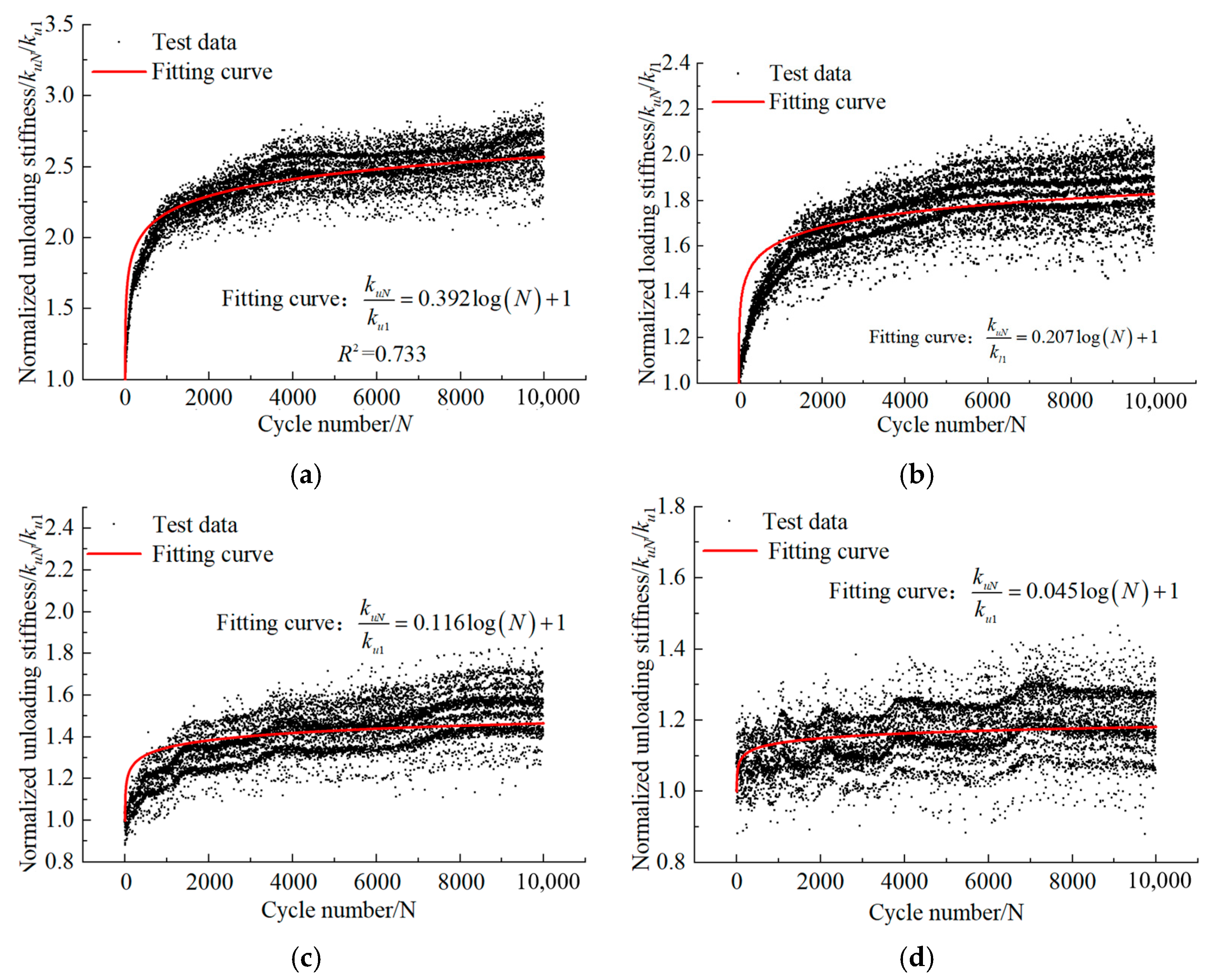
4.4. Prediction Formula of Inclined Cyclic Unloading Stiffness

This study on the variation of pile stiffness under inclined cyclic unloading builds upon the results of horizontal cyclic unloading studies by Chen et al. [21], as presented in Equation (20).

$${\gamma }_u=(-0.44\left({\displaystyle \frac{T}{L}}\right)+0.55)\left(-1.29{\zeta }_c+1.02\right)$$

(20)

As shown in Figure 16, the ratio k_uN/k_u1 exhibits a logarithmic relationship with N. Additionally, considering that k_uN/k_u1 equals 1 when N equals 1, the expression for the inclined cyclic unloading stiffness can be established as follows:

$${\displaystyle \frac{k_{uN}}{k_{u1}}}={\gamma }_{\alpha }\log \left(N\right)+1$$

(21)

where γ_α is the cyclic unloading stiffness coefficient for inclined loading piles. Let:

$${\gamma }_{\alpha }=p_2\left({\theta }_{\mathrm{L}}\right){\gamma }_u$$

(22)

where p₂(θ_L) is the coefficient representing the effect of the θ_L on the inclined cyclic unloading stiffness of the pile, and γ_u is the horizontal cyclic loading stiffness coefficient.

The expression for p₂(θ_L) can be derived as follows:

$$p_2\left({\theta }_{\mathrm{L}}\right)={\displaystyle \frac{{\gamma }_{\alpha }}{{\gamma }_u}}$$

(23)

The summary of the fitting curve results of the relationship between k_uN/k_u1 and N in Figure 17 is shown in

Table 7. Summary of k_uN/k_u1 fitting expressions.

ID	ζb	ζc	T/L	θL (rad)	γu	Fitting Formula	γα	γα/γu
A-1	0.5	0.2	0.190	0	0.355	${\displaystyle \frac{k_{uN}}{k_{u1}}}=0.392\log \left(N\right)+1$	0.392	1.103
A-2	0.5	0.2	0.190	0.349	0.355	${\displaystyle \frac{k_{uN}}{k_{u1}}}=0.207\log \left(N\right)+1$	0.207	0.582
A-3	0.5	0.2	0.190	0.698	0.355	${\displaystyle \frac{k_{uN}}{k_{u1}}}=0.116\log \left(N\right)+1$	0.116	0.326
A-4	0.5	0.2	0.190	1.047	0.355	${\displaystyle \frac{k_{uN}}{k_{u1}}}=0.045\log \left(N\right)+1$	0.045	0.127
A-5	0.5	0.2	0.190	1.396	0.355	${\displaystyle \frac{k_{uN}}{k_{u1}}}=0.054\log \left(N\right)+1$	0.054	0.152
B-1	0.5	0.2	0.375	0	0.293	${\displaystyle \frac{k_{uN}}{k_{u1}}}=0.434\log \left(N\right)+1$	0.434	1.479
B-2	0.5	0.2	0.375	0.349	0.293	${\displaystyle \frac{k_{uN}}{k_{u1}}}=0.222\log \left(N\right)+1$	0.222	0.757
B-3	0.5	0.2	0.375	0.698	0.293	${\displaystyle \frac{k_{uN}}{k_{u1}}}=0.137\log \left(N\right)+1$	0.137	0.467
B-4	0.5	0.2	0.375	1.047	0.293	${\displaystyle \frac{k_{uN}}{k_{u1}}}=0.043\log \left(N\right)+1$	0.043	0.147
B-5	0.5	0.2	0.375	1.396	0.293	${\displaystyle \frac{k_{uN}}{k_{u1}}}=0.019\log \left(N\right)+1$	0.033	0.112

, and the relationship between p₂(θ_L) and θ_L is plotted (as shown in Figure 17).

It can be seen from Figure 17 that the k_uN/k_u1 is obviously correlated with θ_L, and the expression of p₂(θ_L) can be obtained by fitting it as follows:

$${\displaystyle \frac{{\gamma }_{\alpha }}{{\gamma }_u}}=0.7{\theta }_L^2-1.81{\theta }_L+1.29$$

(24)

Combining Equations (20), (22), and (24), the γ_α is obtained as follows:

$${\gamma }_{\alpha }=(-0.44\left({\displaystyle \frac{T}{L}}\right)+0.55)\left(-1.29{\zeta }_c+1.02\right)\left(0.7{\theta }_L^2-1.81{\theta }_L+1.29\right)$$

(25)

By substituting Equation (25) into Equation (21), the following prediction formula for the inclined cyclic unloading stiffness is derived:

$${\displaystyle \frac{k_{uN}}{k_{u1}}}=\left[(-0.44\left({\displaystyle \frac{T}{L}}\right)+0.55)\left(-1.29{\zeta }_c+1.02\right)\left(0.7{\theta }_L^2-1.81{\theta }_L+1.29\right)\right]\log \left(N\right)+1$$

(26)

To verify the validity of Equation (26), several representative numbers of cycles were selected. Using Equation (26), the experimental parameters in Table 7 were calculated to obtain the k_uN/k_u1 values for each group, which were then compared with the actual test data of k_uN/k_u1. The results are shown in

Table 8. Summary table of Equations (19) and (26).

Verify the Summary Table of Equation (19)					Verify the Summary Table of Equation (26)
A-1	N	Test Data klN/kl1	Equation (19) klN/kl1	Error Rate (%)	A-3	N	Test Data kuN/ku1	Equation (26) kuN/ku1	Error Rate (%)
	1000	3.413	3.124	−8.47		1000	1.253	1.173017	11.05
	2000	3.494	3.337	−4.49		2000	1.335	1.190379	7.25
	5000	3.762	3.619	−3.8		5000	1.55	1.213329	−4.29
	10,000	3.689	3.832	3.88		10,000	1.497	1.23069	1.74
A-2	N	Test Data klN/kl1	Equation (19) klN/kl1	Error Rate (%)	A-4	N	Test Data kuN/ku1	Equation (26) kuN/ku1	Error Rate (%)
	1000	2.048	2.304	12.49		1000	1.171	1.173	0.13
	2000	2.158	2.435	12.82		2000	1.093	1.190	8.91
	5000	2.377	2.608	9.69		5000	1.111	1.213	9.22
	10,000	2.628	2.738	4.19		10,000	1.271	1.231	−3.16
B-1	N	Test Data klN/kl1	Equation (19) klN/kl1	Error Rate (%)	B-2	N	Test Data kuN/ku1	Equation (26) kuN/ku1	Error Rate (%)
	1000	4.863	4.44	−8.69		1000	1.54	1.654	7.46
	2000	5.246	4.786	−8.78		2000	1.655	1.720	3.96
	5000	4.993	5.242	−5		5000	1.839	1.807	−1.73
	10,000	5.556	5.587	0.5		10,000	1.885	1.873	−0.64
B-3	N	Test Data klN/kl1	Equation (19) klN/kl1	Error Rate (%)	B-4	N	Test Data kuN/ku1	Equation (26) kuN/ku1	Error Rate (%)
	1000	1.682	1.677	−0.3		1000	1.088	1.143	5.03
	2000	1.831	1.745	−4.69		2000	1.188	1.157	−2.64
	5000	1.839	1.835	−0.2		5000	1.173	1.176	0.25
	10,000	1.737	1.903	9.58		10,000	1.224	1.190	−2.77
B-5	N	Test Data klN/kl1	Equation (19) klN/kl1	Error Rate (%)	B-5	N	Test Data kuN/ku1	Equation (26) kuN/ku1	Error Rate (%)
	1000	1.638	1.634	−0.3		1000	1.132	1.112	−1.78
	2000	1.621	1.697	4.7		2000	1.164	1.123	−3.46
	5000	1.691	1.781	5.33		5000	1.134	1.138	3.95
	10,000	1.625	1.845	13.57		10,000	1.138	1.15	1.04

.

As shown in Table 8, all errors are below 15%, confirming the validity of the prediction formula for the inclined cyclic loading and unloading/stiffness established in this study.

5. Conclusions

Based on existing research on the cumulative displacement and bearing characteristics of horizontally cyclically loaded piles, this study further conducted 10,000 inclined cyclic loading tests on model piles under the influence of different loading angles. Based on the inclined cyclic bearing characteristics of pile foundations, fitting methods for prediction formulas of inclined cyclic cumulative deformation, loading stiffness, and unloading stiffness were proposed. The following conclusions were subsequently drawn:

• A smaller cyclic load angle (θ_L) or larger pile–soil relative stiffness (T/L) results in a greater range and deeper depth of settlement of sandy soil at the pile–soil interface after 10,000 cyclic loadings.
• The cumulative deformation, loading stiffness k_lN/k_l1, and unloading stiffness k_uN/k_u1 of the pile under inclined cyclic loading increase with the number of cycles N, but the rate of increase slows down over time. The larger the θ_L, the faster the initial development of all.
• As θ_L increases from 0° to 80°, the initial peak displacement at the pile top decreases, while the final cumulative displacement first decreases and then increases. Additionally, after 10,000 cycles, the k_lN/k_l1 and k_uN/k_u1 values of slender piles first decrease and then increase, while the k_lN/k_l1 and k_uN/k_u1 values of semi-rigid piles gradually decrease. When θ_L = 80°, k_lN/k_l1 and k_uN/k_u1 values peaked at the initial loading stage.

This study offers a more comprehensive method for predicting inclined cyclic cumulative deformation, loading stiffness, and unloading stiffness of a pile under prolonged cyclic loading conditions, considering different cycle inclined angles. However, the current study does not take into account the different relative density of sand (D_r) and the mechanical characteristics of inclined piles. These factors will be key areas for future research.

References

1. Li, X.; Dai, G.; Zhu, M.; Wang, L.; Liu, H. A Simplified Method for Estimating the Initial Stiffness of Monopile—Soil Interaction Under Lateral Loads in Offshore Wind Turbine Systems. China Ocean Eng. 2023, 37, 165–174. [Google Scholar] [CrossRef]
2. Qin, W.; Gao, J.; Chang, K.; Dai, G.; Wei, H. Set-up effect of large-diameter open-ended thin-walled pipe piles driven in clay. Comput. Geothecnics. 2023, 159, 105459. [Google Scholar] [CrossRef]
3. Qin, W.; Ye, C.; Gao, J.; Dai, G.; Wang, D.; Dong, Y. Pore water pressure of clay soil around large-diameter open-ended thin-walled pile (LOTP) during impact penetration. Comput. Geotech. 2025, 180, 107065. [Google Scholar] [CrossRef]
4. Liu, H.; Zhu, M.; Li, X.; Dai, G.; Yin, Q.; Liu, J.; Ling, C. Experimental study on shear behavior of interface between different soil materials and concrete under variable normal stress. Appl. Sci. 2022, 12, 11213. [Google Scholar] [CrossRef]
5. Qin, W.; Li, X.; Dai, G.; Hu, P. Analytical Penetration Solutions of Large-Diameter Open-Ended Piles Subjected to Hammering Loads. J. Mar. Sci. Eng. 2022, 10, 885. [Google Scholar] [CrossRef]
6. Liu, J.; Zhu, M.M.; Li, X.; Lin, C.; Wang, T.F. The Shear Effect of Large-Diameter Piles under Different Lateral Loading Levels: The Transfer Matrix Method. Buildings 2024, 14, 1448. [Google Scholar] [CrossRef]
7. Li, X.; Dai, G.; Zhu, M.; Zhu, W.; Zhang, F. Investigation of the soil deformation around laterally loaded deep foundations with large diameters. Acta Geotech. 2024, 19, 2293–2314. [Google Scholar] [CrossRef]
8. Hettler, A. Deformations of Stiff and Elastic Foundation Structures in Sand Under Monotonous and Cyclic Loading; Bodenmechanik und Felsmechanik der Universität Fridericiana: Karlsruhe, Germany, 1981; p. 9. [Google Scholar]
9. Lin, S.; Liao, J. Permanent strains of piles in sand due to cyclic lateral loads. J. Geotech. Geoenviron. Eng. 1999, 125, 798–802. [Google Scholar] [CrossRef]
10. Bai, X.Y.; Zhang, Y.J.; Yan, N.; Liu, J.W.; Zhang, Y.M. Experimental investigation on bearing capacity of rock-socketed bored piles in silty clay stratum in beach areas. Appl. Ocean Res. 2025, 154, 104336. [Google Scholar] [CrossRef]
11. Huang, L.; Qin, W.; Dai, G.; Zhu, M.; Liu, L.; Huang, L.; Yang, S.; Ge, M. Ground settlement prediction for highway subgrades with sparse data using regression Kriging. Sci. Rep. 2024, 14, 24594. [Google Scholar] [CrossRef] [PubMed]
12. Wang, J.; Jin, T.; Qin, W.; Zhang, F. Performance evaluation of post-grouting for bored piles installed in inhomogeneous gravel pebble stratum overlaid by deep and soft soil layers. Geomech. Geoengin. Int. J. 2024, 19, 77–95. [Google Scholar] [CrossRef]
13. Qin, W.; Cai, S.; Dai, G.; Wang, D.; Chang, K. Soil Resistance during Driving of Offshore Large-Diameter Open-Ended Thin-Wall Pipe Piles Driven into Clay by Impact Hammers. Comput. Geotech. 2023, 153, 105085. [Google Scholar] [CrossRef]
14. LeBlanc, C.; Houlsby, G.T.; Byrne, B.W. Response of stiff piles in sand to long-term cyclic lateral loading. Géotechnique 2010, 60, 79–90. [Google Scholar] [CrossRef]
15. Leblanc, C.; Byrne, B.W.; Houlsby, G.T. Response of stiff piles to random two-way lateral loading. Géotechnique 2010, 60, 715–721. [Google Scholar] [CrossRef]
16. Lin, J.Y. Study on the Evolution of Bearing Performance and Cumulative Deformation Characteristics of Monopiles Under Horizontal Cyclic Loading. Master’s Thesis, Southeast University, Nanjing, China, 2021. [Google Scholar]
17. Wang, Y.; Zhu, M.X.; Dai, G.L.; Gong, W.M.; Lin, J.Y. Characteristics of cumulative deformation and prediction method for pile foundation under cyclic lateral loading considering influences of pile-soil relative stiffness. J. Geotech. Eng. 2022, 44, 220–225. [Google Scholar]
18. Rathod, D.; Nigitha, D.; Krishnanunni, K.T. Experimental Investigation of the Behavior of Monopile under Asymmetric Two-Way Cyclic Lateral Loads. Int. J. Geomech. 2021, 21, 06021001. [Google Scholar] [CrossRef]
19. Liang, R.; Yuan, Y.; Fu, D.S.; Liu, R. Cyclic response of monopile-supported offshore wind turbines under wind and wave loading in sand. Mar. Georesources Geotechnol. 2021, 39, 1230–1243. [Google Scholar] [CrossRef]
20. Li, Q.; Askarinejad, A.; Gavin, K. Lateral response of rigid monopiles subjected to cyclic loading: Centrifuge modelling. Proc. Inst. Civ. Eng.-Geotech. Eng. 2020, 175, 426–438. [Google Scholar] [CrossRef]
21. Chen, J.; Shu, J.; Xi, S.; Gu, X.; Zhu, M.; Li, X. A New Method for Predicting Dynamic Pile Head Stiffness Considering Pile-Soil Relative Stiffness Under Long-Term Cyclic Loading Conditions. Buildings 2024, 14, 3483. [Google Scholar] [CrossRef]
22. Li, X.; Zhu, M.; Dai, G.; Wang, L.; Liu, J. Interface Mechanical Behavior of Flexible Piles Under Lateral Loads in OWT Systems. China Ocean Eng. 2023, 37, 484–494. [Google Scholar] [CrossRef]
23. Li, X.; Dai, G. Closure to “Energy-Based Analysis of Laterally Loaded Caissons with Large Diameters under Small-Strain Conditions”. Int. J. Geomech. 2023, 23, 07023008. [Google Scholar] [CrossRef]
24. Reese, L.C.; Cox, W.R.; Koop, F.D. Analysis of Laterally Loaded Piles in Sand. In Proceedings of the 6th Annual Offshore Technology Conference, Houston, TX, USA, 5–7 May 1974; pp. 473–483. [Google Scholar]
25. Reese, L.C.; Welch, R.C. Lateral loading of deep foundations in stiff clay. J. Geotech. Geoenviron. Eng. 1975, 101, 633–649. [Google Scholar] [CrossRef]
26. Cuéllar, P. Pile foundations for offshore wind turbines: Numerical and Experimental Investigations on the Behaviour Under Short-Term and Long-Term Cyclic Loading. Ph.D. Thesis, der Technischen Universität Berlin, Berlin, Germany, 2011. [Google Scholar]
27. Abadie, C.N.; Byrne, B.W.; Houlsby, G.T. Rigid pile response to cyclic lateral loading: Laboratory tests. Géotechnique 2019, 69, 863–876. [Google Scholar] [CrossRef]
28. Zhang, X.; Huang, M.S.; Hu, Z.P. Modeling test of horizontal cyclic cumulative deformation characteristics of single pile in sandy soil. Geotechnics 2019, 40, 933–941. [Google Scholar]
29. Sun, Y.X. Horizontal Bearing Characteristics Test and Numerical Analysis of Large Diameter Single Pile for Offshore Wind Turbine. Ph.D. Thesis, Zhejiang University, Hangzhou, China, 2017. [Google Scholar]
Figure 1. Cyclic loading system. (a) Loading device diagram; (b) test model box.
Buildings 15 00591 g001
Figure 2. Particle gradation curve.
Buildings 15 00591 g002
Figure 3. Stress sheet pasting and calibration of model piles. (a) Diagram of strain gauge and loading point; (b) calibration of model piles; and (c) calibration test data.
Buildings 15 00591 g003aBuildings 15 00591 g003b
Figure 4. The U.S. ACE manual provides the recommended value for nh.
Buildings 15 00591 g004
Figure 5. Schematic diagram of the model pile being uplifted. (a) Pre-test; (b) after several cycles.
Buildings 15 00591 g005
Figure 6. A-pile inclination cyclic loading test. (a) A-2 (θL = 20°) test before; (b) A-2 (θL = 20°) test after; (c) A-3 (θL = 40°) test before; (d) A-3 (θL = 40°) test after; (e) A-4 (θL = 60°) test before; (f) A-4 (θL = 60°) test after; (g) A-5 (θL = 80°) test before; and (h) A-5 (θL = 80°) test after.
Buildings 15 00591 g006aBuildings 15 00591 g006b
Figure 7. B-pile inclination cyclic loading test. (a) A-2 (θL = 20°) test before; (b) A-2 (θL = 20°) test after; (c) A-3 (θL = 40°) test before; (d) A-3 (θL = 40°) test after; (e) A-4 (θL = 60°) test before; (f) A-4 (θL = 60°) test after; (g) A-5 (θL = 80°) test before; and (h) A-5 (θL = 80°) test after.
Buildings 15 00591 g007aBuildings 15 00591 g007b
Figure 8. Inclination cyclic Q-s curves. (a) A-1 (θL = 0°); (b) A-2 (θL = 20°); (c) A-3 (θL = 40°); (d) A-4 (θL = 60°); (e) A-5 (θL = 80°); (f) B-1 (θL = 0°); (g) B-2 (θL = 20°); (h) B-3 (θL = 40°); (i) B-4 (θL = 60°); and (j) B-5 (θL = 80°).
Buildings 15 00591 g008aBuildings 15 00591 g008b
Figure 9. Relationship between yN/y1 and N. (a) Pile A; (b) pile B.
Buildings 15 00591 g009
Figure 10. Normalized log–log curve of cumulative displacements. (a) Pile A; (b) pile B.
Buildings 15 00591 g010
Figure 11. p(θL) expression fitting.
Buildings 15 00591 g011
Figure 12. Verification of Equation (8).
Buildings 15 00591 g012
Figure 13. The definition diagram of two kinds of stiffness.
Buildings 15 00591 g013
Figure 14. Relationship between klN/kl1 and N. (a) A-1 (θL = 0°); (b) A-2 (θL = 20°); (c) A-3 (θL = 40°); (d) A-4 (θL = 60°); (e) A-5 (θL = 80°); (f) B-1 (θL = 0°); (g) B-2 (θL = 20°); (h) B-3 (θL = 40°); (i) B-4 (θL = 60°); and (j) B-5 (θL = 80°).
Buildings 15 00591 g014aBuildings 15 00591 g014b
Figure 15. p1(θL) expression fitting.
Buildings 15 00591 g015
Figure 16. Relationship between kuN/ku1 and N. (a) A-1 (θL = 0°); (b) A-2 (θL = 20°); (c) A-3 (θL = 40°); (d) A-4 (θL = 60°); (e) A-5 (θL = 80°); (f) B-1 (θL = 0°); (g) B-2 (θL = 20°); (h) B-3 (θL = 40°); (i) B-4 (θL = 60°); and (j) B-5 (θL = 80°).
Buildings 15 00591 g016aBuildings 15 00591 g016b
Figure 17. p2(θL) expression fitting.
Buildings 15 00591 g017