Abstract
Traditional monolithic precast and precast prestressed concrete joints often face challenges such as complex steel reinforcement details and low construction efficiency. Grouting sleeve connections may also suffer from quality issues. To address these problems, a new precast prestressed concrete frame beam-column exterior joint using ultra-high-performance concrete (UHPC) for connection (PPCFEJ-UHPC) is proposed. This innovative joint lessens the amount of stirrups in the core area, decreases the anchorage length of beam longitudinal reinforcement, and enables efficient lap splicing of column longitudinal reinforcement, thereby enhancing construction convenience. Cyclic loading tests were conducted on three new exterior joint specimens (PE1, PE2, PE3) and one cast-in-place joint specimen (RE1) to evaluate their seismic performance. The study concentrated on failure modes, energy dissipation capacity, displacement ductility, strength and stiffness degradation, shear stress, and deformation’s influence on the longitudinal reinforcement anchoring length and axial compression ratio. The results indicate that the new joint exhibits beam flexural failure with minimal damage to the core area, unlike the cast-in-place joint, which suffers severe core area damage. The novel joint exhibits at least 21.7% and 6.1% improvement in cumulative energy consumption and ductility coefficient, respectively, while matching the cast-in-place joint’s bearing capacity. These characteristics are further improved by 5.5% and 10.7% when the axial compression ratio is increased. The new joints’ seismic performance indices all satisfy the ACI 374.1-05 requirements. Additionally, UHPC significantly improves the anchoring performance of steel bars in the core area, allowing the anchorage length of beam longitudinal bars to be reduced from 16 times of the diameter of reinforcement to 12 times.
1. Introduction
To allow structural parts to reach their maximum strength and ductility, in reinforced concrete (RC) constructions, beam-column joints—areas where structural elements intersect—need to be shielded from early collapse [1]. Many papers focus on the shear transfer mechanism, capacity models, and the failure mechanism while studying the beam-column joints’ seismic performance [2,3,4,5,6,7]. However, there are still many limitations to normal concrete joints. Researchers have turned their attention to new types of joints, both structural forms and materials.
Precast concrete structures have gained popularity due to their high construction efficiency, modular production, and reduced energy consumption [8,9,10,11,12]. Incorporating prestressing technology into precast concrete structures combines the benefits of both prestressed and precast systems [13,14,15]. Pretensioned prestressing enhances crack resistance, reduces cross-sections, and minimizes the number of supports, making it suitable for large-span and heavy-duty structures [16,17,18,19,20,21,22].
UHPC has been used in a variety of structural applications [23,24,25,26,27,28] due to its compressive strength of at least 120 MPa [29], shear strength of 20 MPa [30], and average bond strength of at least 20 MPa [31]. Its application in the central region of prefabricated pre-stressed beam-column joints has not yet been investigated, however. UHPC’s high shear and bond strengths make it ideal for ensuring “strong joint, weak member” principles, effectively overlapping steel bars, and addressing grouting sleeve issues. Unlike interior joints, exterior joints have only one beam end, making the anchorage performance of beam longitudinal reinforcement crucial. UHPC ensures effective anchorage, reducing the required anchorage length. While steam curing is common for UHPC, room temperature curing is more practical, though it may cause shrinkage and interface damage. A type of precast prestressed concrete beam-column interior joint using UHPC for connection (PPCFIJ-UHPC) was tested, and the results showed that it had good mechanic and seismic performance [32].
This study proposes a new precast prestressed concrete frame exterior joint using UHPC (PPCFEJ-UHPC) and investigates its seismic performance under low-cycle repeated loads.
In the first two paragraphs of the narrative, the same type of interior joint using UHPC for connection were tested [32], and the performance of the interior joint and exterior joint was significantly different. Exterior joint carries forces from three directions, while the interior joint carries four. It makes peak loads of PPCFEJ-UHPC larger than that of PPCFIJ-UHPC. Due to its relatively simple structure, the anchorage length can also be relatively small (it is suggested to be 12db, while some tests [33] took 16db, and the author’s previous work did not discuss this question), resulting in better seismic performance.
2. Experimental Description
2.1. Design Specimens
Three PPCFEJ-UHPC exterior joints and one cast-in-place exterior joint were designed. The new joint features a prefabricated pre-tensioned prestressed composite beam with longitudinal bars and steel strands anchored in the core area. UHPC was poured into the joint core area under normal temperature curing. The beam and column sections were 230 mm × 450 mm and 360 mm × 360 mm, respectively, using HRB400 grade steel bars and 1860 grade steel strands. The concrete design strength was C50, with UHPC used in the core area of beam-column joint.
The prototype of the test piece design is a four-layer bus parking lot in Pudong, Shanghai. It is a reinforced concrete frame structure. Due to its large span, heavy load, and high floor height, a prefabricated prestressed concrete frame scheme with less support is considered for this structure. The main beam adopts pretensioned precast concrete beams, which can bear the construction and structural weight, reducing the number of supports used. The building has a height of 23 m, with the first floor being a height of 6.35 m, the second and third floors being a height of 5.5 m, and the fourth floor being a height of 5.65 m. The X direction span is 14.4 m, and the span in the Y direction is 12.8 m. The secondary beam is arranged along the X direction. Prestressed concrete beams measuring 600 × 1300 mm in cross-section and columns measuring 800 × 1000 mm in cross-section make up the original structural frame. According to the laboratory conditions, the scale ratio of the joint specimen is determined to be 1:3. After relevant adjustments, the size of the middle and edge joint beams was determined to be 230 × 450 mm, and the height of the composite layer is 100 mm.
The beam section size of each specimen is 230 mm × 450 mm, and the column section size is 360 mm × 360 mm. The common steel bars and stirrups are HRB400 grade steel bars, and the prestressed bars are 1860 grade steel strands. Normal concrete with a design strength of C50 was used to pour the beams and columns, while UHPC was used to pour the joints’ core area. Table 1 displays the design parameters, while Figure 1 displays the specimen’s size and reinforcement. The specimen PE1 has a design axial compression ratio of 0.067 and a test axial compression ratio of 0.034.
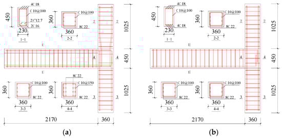
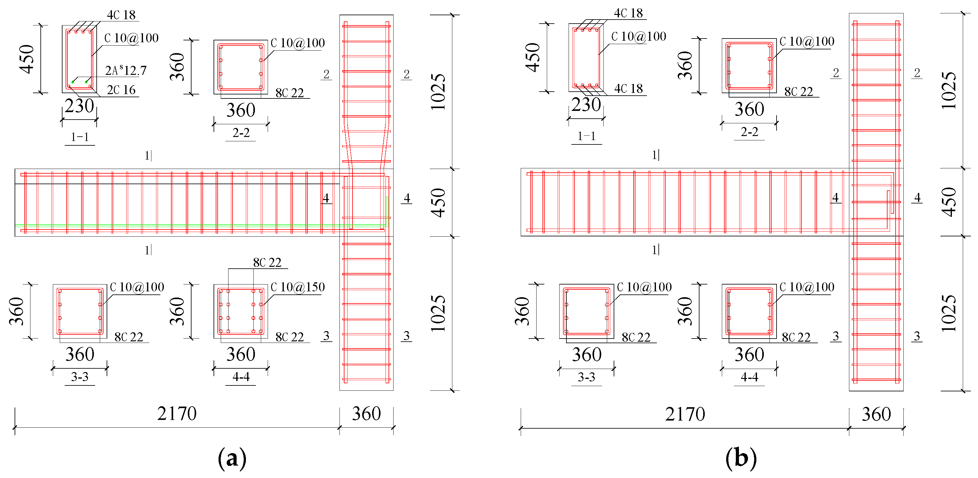
Figure 1.
Reinforcement details of specimens (mm). (a) New exterior joint specimens. (b) Cast-in-place exterior joint specimen.
Some tests have shown that the steel bars’ anchorage length with a diameter of 22 mm in UHPC is only 18db [34]. The diameters of the beam longitudinal bars in this test are 18 mm and 16 mm. Conservatively, the specimens were 18db and 20db, respectively, for the beam longitudinal steel bars anchorage length in the core area poured by UHPC. For the anchorage length of steel strands, the literature [35,36] suggested that the steel strands anchorage lengths in UHPC should be 35db and 40db, respectively, and 40db was conservatively selected in this test. The tests in refs. [37,38] yielded a limit lap length of 10db to 13db for the longitudinal strengthening of the column, and this test was conservatively taken as 16db. In the test, all anchorage lengths were taken conservatively so that slippage of steel bars and steel strands did not happen.

Table 1.
Specimen parameters.
Table 1.
Specimen parameters.
| Specimen | L1 | Beam Bottom Bars | L2 | L3 | Stirrups of the Core Area | Materials in the Core Area | Design Axial Compression Ratio |
|---|---|---|---|---|---|---|---|
| RE1 | 18db + 15db | 4C18 | 18db + 15db | — | 0.48% | NC | 0.067 |
| PE1 | 18db | 2As12.7 + 2C16 | 20db | 25db + 15db | 0.32% | UHPC | 0.067 |
| PE2 | 18db | 2As12.7 + 2C16 | 20db | 25db + 15db | 0.32% | UHPC | 0.2 |
| PE3 | 18db + 15db | 2As12.7 + 2C16 | 20db + 15db | 25db + 15db | 0.32% | UHPC | 0.067 |
Notes: (1) UHPC and NC represent ultra-high performance concrete and concrete, respectively; (2) The top reinforcement of each specimen is 4C18, one side of the column has 4C22 reinforcement, and the new joint’s lap length for the longitudinal reinforcement of the column is 16db; (3) The length of the straight section plus the length of the bending section—of which, the predicted length of the bending section is 15db—is the anchoring length of the steel bar and steel strand, and it consists of 12db straight length and 3db hook length specified in GB50010 “Code for Design of Concrete Structures” [39]; (4) L1 stands for the longitudinal bars’ anchorage length at the top of the beam, L2 for the longitudinal bars’ anchorage length at the bottom, and L3 for the steel strand’s anchorage length at the bottom.
The construction sequence of the new joint and some pictures of construction are shown in Figure 2. Step 1: Pretensioned prestressed beams and the upper and lower columns should be prefabricated. For lap jointing in the joint’s central region, longitudinal bars are extended in both the upper and lower columns. The beam’s steel strands and longitudinal reinforcement reach into the joint’s core, and the end of the longitudinal reinforcement bends to strengthen the anchorage. Step 2: The lower column is fixed and the stirrups are installed in the core area of the joint, the upper column is installed and the stirrups are bound, and then the prefabricated pretensioned beam is placed in the joint’s core, with the longitudinal reinforcement of the superimposed layer arranged on the top portion of the beam. Step 3: The normal concrete is poured over the UHPC and beam superimposed layer.
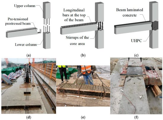
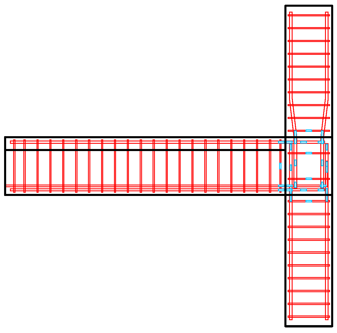
Figure 2.
Construction sequence of the new joints. (a) Step 1; (b) Step 2; (c) Step 3; (d) tension steel strand; (e) pouring the beam and column; (f) pouring the joint and superimposed layer.
2.2. Material Property
According to GB/T 50081 “Standards for Test Methods of Physical and Mechanical Properties of Concrete” [40], the axial compressive strengths of NC and UHPC were measured for this test and are displayed in Table 2. Table 3 and Table 4 display the ratios of the NC and UHPC materials used, while Table 5 lists the steel fiber performance metrics. Table 6 lists the kinds of steel bars and steel strands used in the specimens, together with their related mechanical parameters (measured in accordance with JGJ 369-2016, “Code for design of prestressed concrete structures” [41]).
Table 2.
Mechanical properties of NC and UHPC.
Table 3.
Mixture proportions of NC.
Table 4.
Mixture proportions of UHPC.
Table 5.
Performance indicators of steel fibers.
Table 6.
Steel bars and steel strands’ mechanical properties.
2.3. Test Procedure
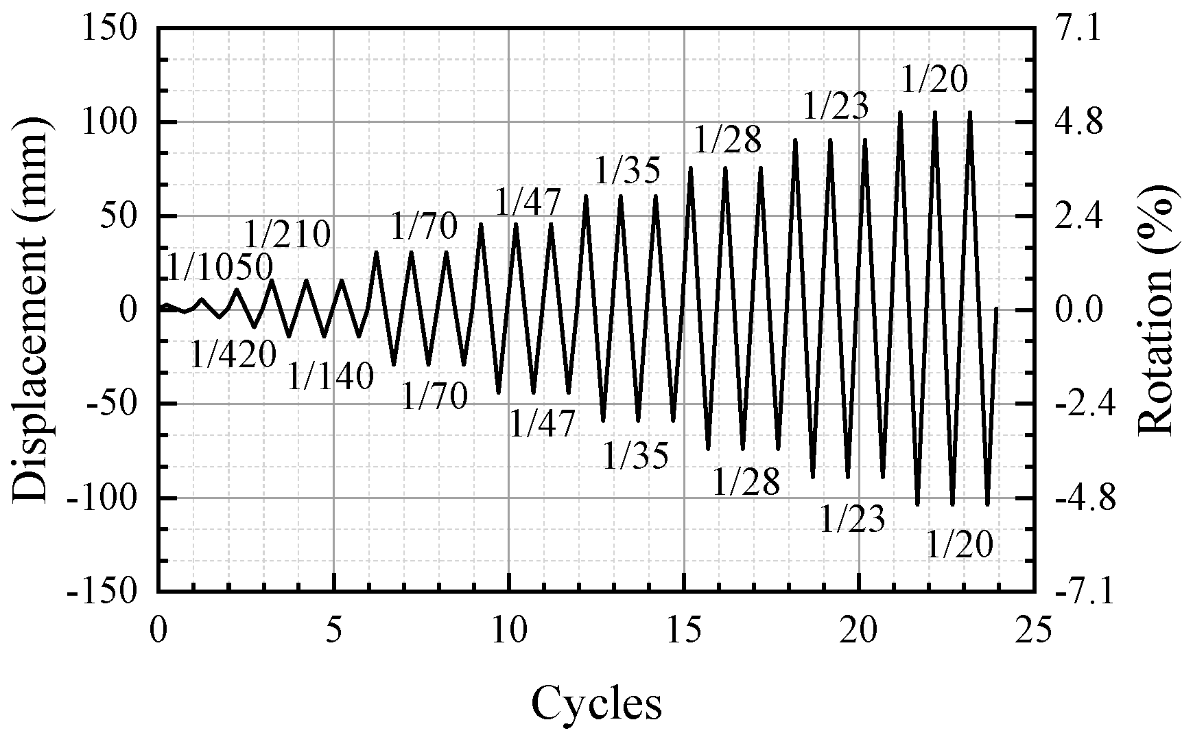
Figure 3 displays the configuration for this test. The columns’ tops and bottoms are joined by fixed hinge supports. An actuator is installed above the column to guarantee the consistent force. The top of the column experiences continuous axial pressure during beam end loading. The MTS1000kN servo actuator (Beijing Fluid Control System Corp., Beijing, China) controls the vertical repeated load at the beam end, whereas the MTS1500kN servo actuator (Beijing R&F Tongda Technology Co., Ltd., Beijing, China) controls the vertical constant load at the top of the column. The displacement loading method is used in the test. Figure 4 displays the loading system. The ratio of beam end displacement to beam length is known as the rotation. Every level of displacement is cyclically loaded once prior to the specimen yielding, and three times following the specimen’s yielding. If the vertical load of the beam end drops to less than 85% of the peak load, loading is stopped.
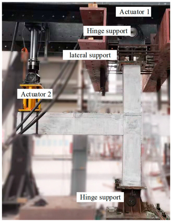
Figure 3.
Diagram of test setup.

Figure 4.
Test loading regime.
2.4. Test Content and Measuring Point Layout
Figure 5 and Figure 6 depict the arrangement of the specimen’s displacement gauge and strain gauge. The test content includes the following aspects: (1) the horizontal displacement at the top and bottom position of column (point 7 and point 8 in Figure 5); (2) the beam end’s vertical displacement (point 1–6, point 9 in Figure 5) (due to the rotation at the root of the beam, the angle of rotation can be measured using 1–6, and this rotational displacement can be subtracted); (3) the core area’s shear deformation of the joint (point 10, point 11 in Figure 5); (4) the steel bar and the steel strand’s strain (strain gauges in Figure 6).
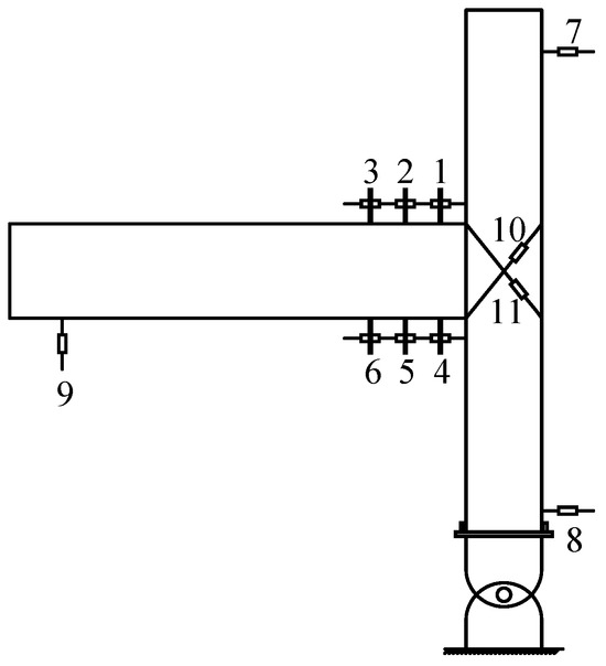
Figure 5.
Displacement measuring point arrangement.
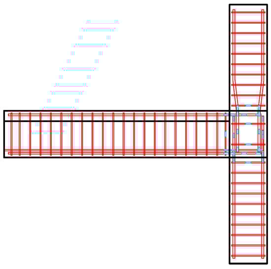
Figure 6.
Placement of strain gauges (blue in the picture).
3. Test Phenomenon and Failure Mode
According to the equivalent energy method [42], the four specimens’ forward and reverse yield and peak loads are listed in Table 7.
Table 7.
The four specimens’ forward and reverse yield loads and peak loads.
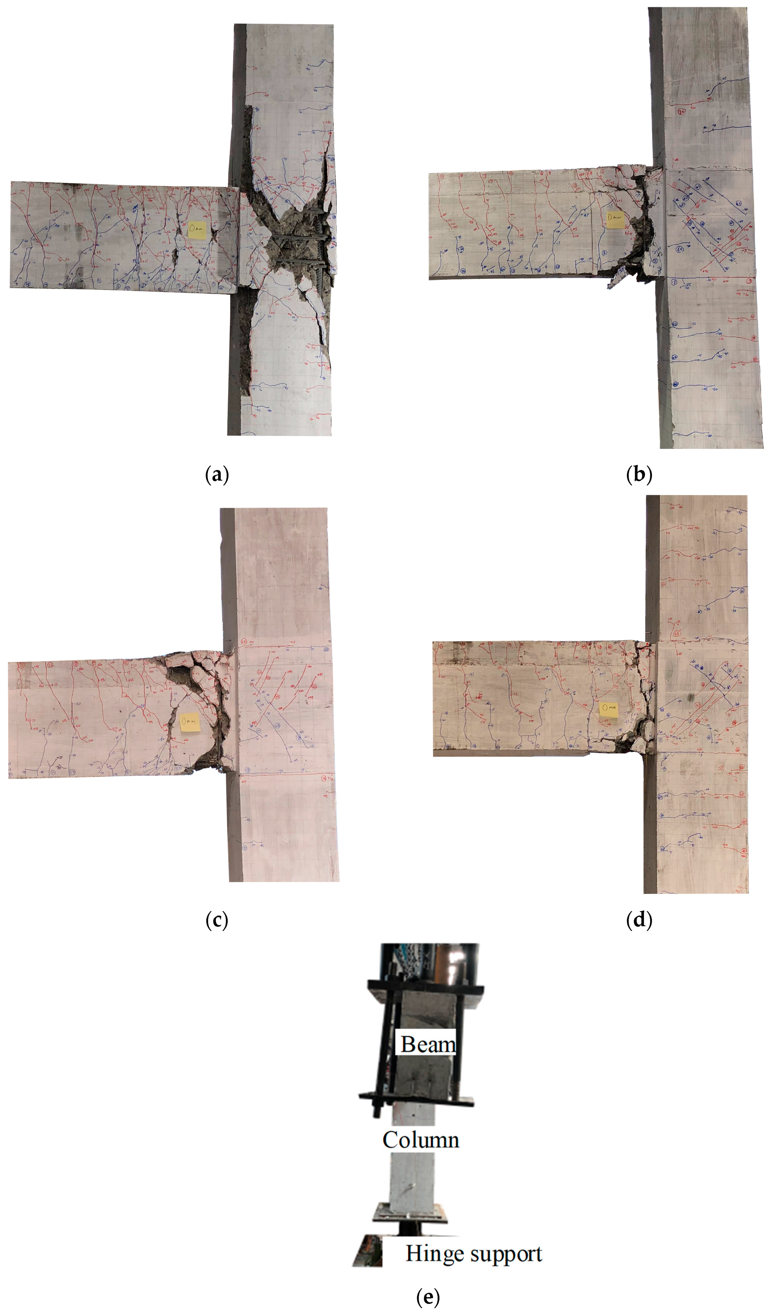
For the cast-in-place specimen RE1, when loaded to the +2 mm level (the beam end angle is 0.10%), two bending cracks were detected at the beam end’s top, and when the reverse loading was at the −2 mm level, four bending cracks appeared at the beam end’s bottom. The fissures at the beam end keep growing as the load increases. When the load reaches the +10 mm level (0.48%), it is assumed that the cracks in the joint core area’s corner that run parallel to the beam’s longitudinal bars are bond anchoring cracks. When the loading reaches the level of 15 mm (0.71%), micro-cross oblique cracks show up in the forward and backward directions of the joint’s core area, whereas micro-cracks show up on the column’s edge. Currently, the core area’s maximum crack width is 0.14 mm. When the displacement is +24.64 mm (1.17%) and −27.60 mm (1.31%), the specimen reaches the forward and reverse yield loads of 88.4 kN and −92.6 kN, respectively. As the loading progresses, shear cracks in the core area and bending cracks at the beam end are still growing. When the loading reaches the 75 mm level (3.57%), the forward and reverse directions of the specimen reach peak loads of 99.4 kN and −109.1 kN, respectively. At this time, the core area of concrete began to peel off, and the stirrups were exposed; when the 90 mm-level loading was completed, the concrete in the core area fell off in a large area, and the protective layer of the pillar corner edge concrete fell off. When loaded to the 105 mm level (5.00%), the specimen’s forward and reverse loads both declined to 85% of the peak load, and the test ended. The longitudinal bars of the beam-column and the stirrups in the joint’s core area all yielded. Shear failure in the joint’s core area following beam end yielding was the specimen’s mode of failure. The joint’s core area was seriously damaged, and the maximum crack width reached 2.5 mm, as shown in Figure 7a.
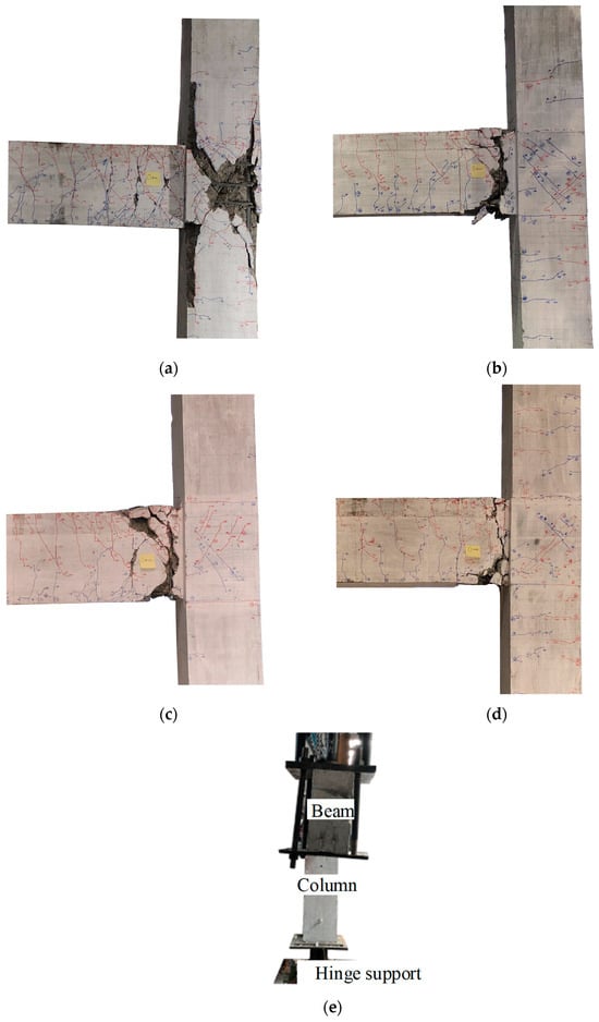
Figure 7.
Failure modes of 4 specimens. (a) RE1. (b) PE1. (c) PE2. (d) PE3. (e) Side view of PE3 loading process.
The pre-tensioned prestressed beams and columns of the standard specimen PE1 are prefabricated. The steel strands are bent anchored, and the longitudinal bars of the beams are directly secured in the joint’s core. The core of the joint is where the column’s longitudinal bars are lapped. The cracking load at the beam end is the same as that of PE1. When the displacement of the beam end reaches the +15 mm level (rotation reaches 0.71%), micro-cracks are observed at the superimposed interface of the beam. When the displacement is +21.67 mm (1.03%) and −25.93 mm (1.23%), the specimens reach the positive and negative yield loads of 86.0 kN and −91.2 kN, respectively. Very tiny cross-oblique cracks with a maximum crack thickness of just 0.02 mm are seen in the front and backward directions of the joint’s core area under loading to the 30 mm level. When loaded to the 60 mm level (2.86%), the specimen’s forward and reverse directions reached the peak loads of 97.1 kN and −112.1 kN, respectively; at this time, a small piece of concrete fell off at the beam’s bottom, when there was almost no crack development in the cylindrical surface and core area.. Following three cyclic loading progress, the concrete at the beam end’s bottom collapsed significantly, and the stirrups were exposed. With the load increases, the concrete at the bottom of the beam end falls off more seriously, and the longitudinal bars and steel strands are gradually exposed. When loaded to the 105 mm level (5.00%), the specimen’s forward and reverse loads both declined to 85% of the peak load and the longitudinal reinforcement at the bottom of the beam was broken, and the test was over. The interface between the beam end and the core area was severely damaged, the longitudinal reinforcement of the column and the stirrups in the core area of the joint did not yield, and the damage in the core area of the joint was minor, with the maximum crack width in the core area being only 0.08 mm. Figure 7b shows PE1’s failure form.
For PE2 and PE3, their stress behavior and failure form were basically the same as those of PE1, and for the sake of simplicity, they will not be described in detail. Figure 7c,d show the failure forms of PE2 and PE3. It should be noted that during the loading process, it was found that the PE3 beam had a torsion phenomenon, which had some influence on its later force, as shown in Figure 7e.
In a word, the cast-in-place joint (RE1) exhibited shear failure in the core area after beam-end yielding, with severe damage of the core area and a maximum crack width of 2.5 mm. The new joints (PE1, PE2, PE3) showed beam flexural failure with minimal core area damage (maximum crack width ≤ 0.08 mm). PE3 experienced beam torsion, affecting its performance.
4. Test Results Analysis
4.1. Hysteresis Curve and Backbone Curve
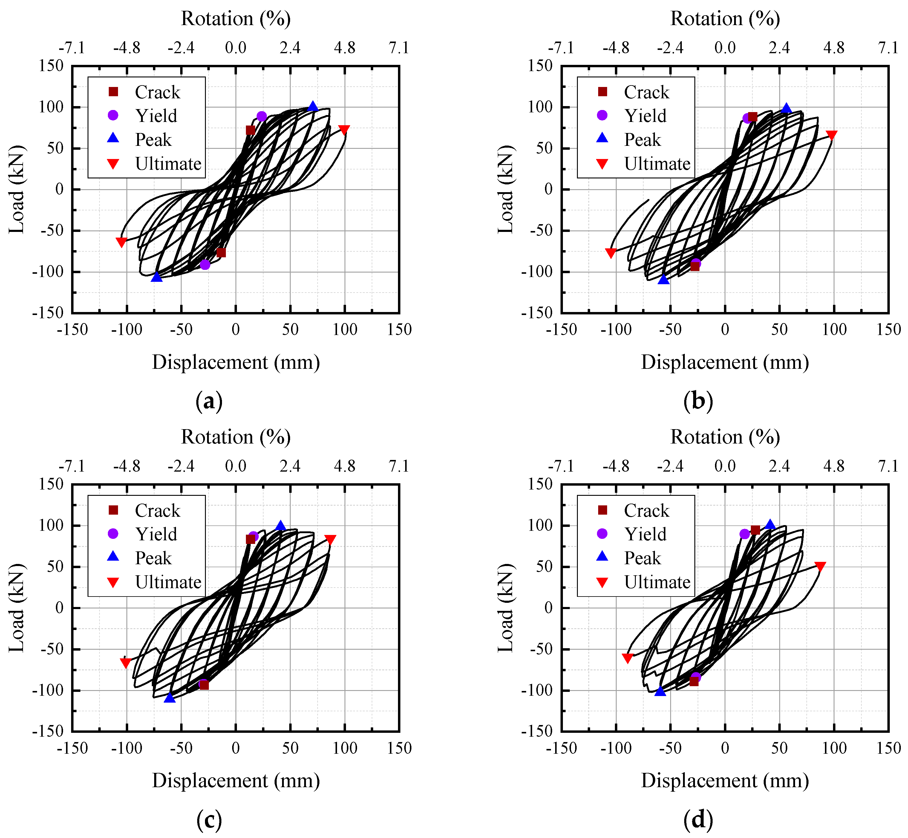
Based on the test results, Figure 8 shows the specimen’s beam end load-displacement hysteresis curve. Among these, the yield point is determined by the equivalent energy technique, and the cracking point is defined as the load that corresponds to the first oblique crack in the joint’s core area [43].
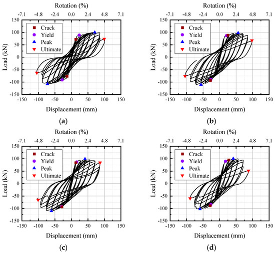
Figure 8.
Load-displacement hysteretic loops. (a) RE1. (b) PE1. (c) PE2. (d) PE3.
For PE1, before the specimen yields, the hysteresis curve is linear, and the beam end loads reach the maximum values of 97.07 kN and −112.1 kN at the corner displacements of 2.73% and −2.65%. Additionally, the PE1’s load-displacement hysteresis curve is extremely complete, and no steel slip phenomenon is found in PE1, indicating that the bond is reliable. For PE2 and PE3, the beam ends were also damaged by bending, and their hysteresis curves resembled PE1’s quite a little. After RE1’s beam-end yielded, shear failure took place in the joint’s core area, and a pinching phenomenon occurred in the later stage of the hysteresis loop. The hysteresis loop was not full, and the energy dissipation performance was deviated.
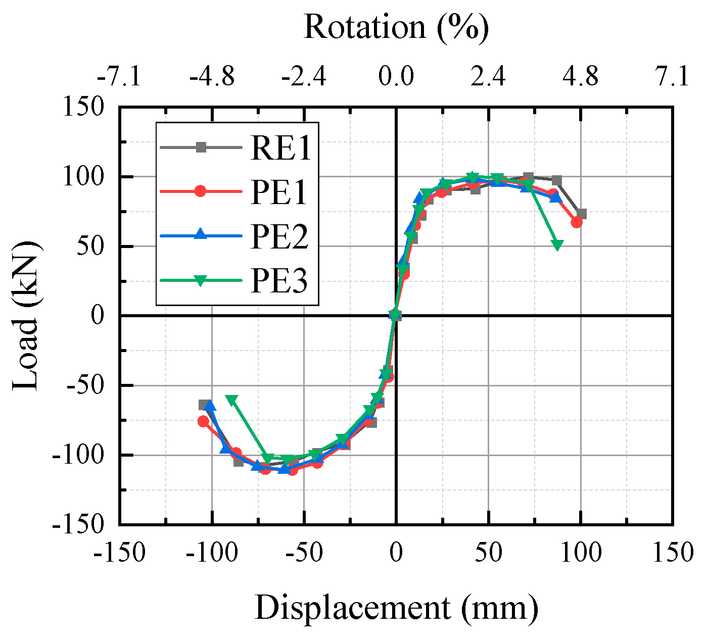
According to Figure 9’s backbone curve, the changing trend of PE1 before yielding is basically the same as that of RE1. After the specimen yields, RE1 had a stable process and then entered the strengthening stage directly. The new joint’s bearing capacity was equal to that of the cast-in-place joint and satisfied the same cast-in-place requirements from the standpoint of bearing capacity, as evidenced by the 2.4% decrease and 2.7% increase in the reverse bearing capacity when compared to RE1. Compared with PE1, PE2 increased the axial compression ratio, and its hysteresis curve was fuller. Because the beam end reinforcement was the same, and the reinforcement was yielded, the bearing capacity of the two specimens was very close, with only a slight increase. The backbone curve’s initial stiffness and bearing capacity for PE3 were essentially the same as those for PE1, but the beam end’s twisting caused the bearing capacity to drop off significantly later on.
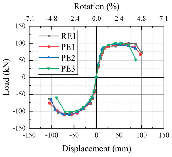
Figure 9.
Specimens’ backbone curves.
The new joints’ load-displacement hysteresis curves were full, indicating reliable bonding. With minor differences in stiffness and strength degradation, the skeleton curves demonstrated that the new joints’ bearing capacities were comparable to those of the cast-in-place joint. A fuller hysteretic curve can be obtained by increasing the axial compression ratio. The specimen’s design (15db) can meet the seismic requirements.
4.2. Energy Dissipation Capacity
One crucial metric for assessing the structure’s seismic performance is its energy dissipation capability. The structure’s energy dissipation capacity under various loading and displacement series was characterized in this research using the equivalent viscous coefficient and cumulative energy dissipation. The specimen’s ability to dissipate energy increases with the value. For each hysteretic loop, the area that each loop encloses can be used to get the equivalent viscous damping coefficient. Figure 10 illustrates the computation process, while Equation (1) displays the calculation formula [43]:
where the equivalent viscous damping coefficient is he; the area of the triangle obf is SΔobf, and the area of the hysteresis loop is Sabcd. The area of the triangle oed is SΔoed. The average value should be used when there are several loading cycles for the same displacement level.
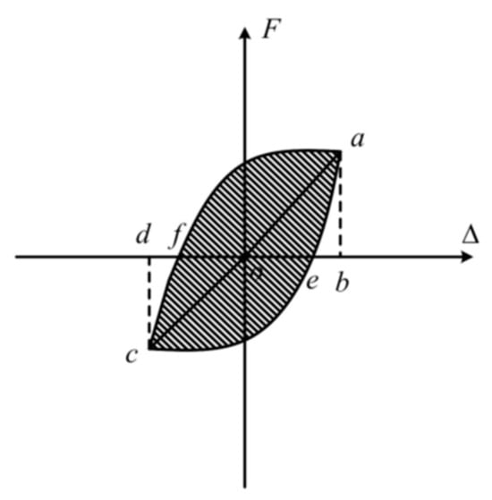
Figure 10.
An example of energy dissipation with a hysteresis loop.
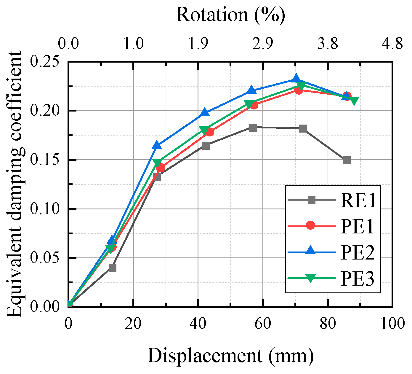
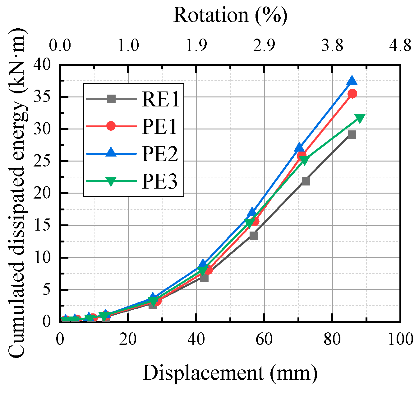
Figure 11 displays the comparable viscous damping coefficient calculation findings for each specimen. During the initial loading phase, with displacement increasing, each specimen’s equivalent viscous damping coefficient progressively rises. The hysteresis damping coefficient steadily drops until the specimen collapses as displacement increases. As far as PE1 and PE1 are concerned, the equivalent viscous damping coefficients of both reach their peaks at the 75 mm level (3.57%), and the latter is 21.6% higher than the former; at the 90 mm level (4.29%), the latter is 43.6% higher than the former, because the RE1 joint undergoes shear failure, the viscous damping coefficient drops sharply, and the beam end is where the majority of PE1’s deformation occurs, so the viscous damping coefficient decreases very little. In addition, as seen in Figure 12, the PE1’s cumulative energy consumption is 21.7% higher than the RE1’s, indicating that the new joint performs substantially better in terms of energy consumption than the cast-in-place joint.
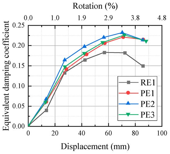
Figure 11.
Equivalent viscous damping coefficient.

Figure 12.
Cumulative dissipated energy.
PE2’s equivalent viscous damping coefficient peak value is 5.0% higher than PE1’s, and its cumulative energy consumption is increased by 5.5%. The axial compression ratio’s ability to increase the joint’s energy dissipation performance is limited because the beam end is bent and damaged. Before the 75 mm relocation, PE3’s cumulative energy consumption was the same as PE1’s, and the peak value of the equivalent viscous damping coefficient was marginally greater, resulting in insufficient cumulative energy consumption, which was 10.5% lower than that of PE1.
4.3. Ductility and Deformation Capacity
One of the key markers to describe a structure’s seismic performance is its ductility, which is the capacity of a structure or component to tolerate inelastic deformation without appreciably lowering its bearing capacity [44]. Beam end loading’s displacement ductility coefficient can express its nodal ductility, and the calculation formula is shown in Equation (2):
where the specimen’s ductility coefficient is μ; Δy is the specimen’s yield displacement, which can be calculated according to the equivalent energy method by backbone curve [45]. When the bearing capacity falls to 85% of the maximum load, the associated displacement is denoted by Δu, as shown in Figure 13.
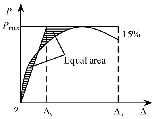
Figure 13.
Schematic diagram of equivalent energy method.
According to Table 8’s forward and reverse average ductility coefficients, each specimen’s ductility coefficient falls between 3.48 and 4.20, which meet and are slightly higher than the ductility coefficients of 3 to 4 required by the structure’s seismic design [46]. The PE1’s ductility coefficient is 6.1% greater than the RE1’s, indicating that the new joint performs better in terms of ductility than the RE1. The PE2’s ductility coefficient is 10.7% higher than that of the PE1, suggesting that raising the axial compression ratio within a specific range enhances the joint’s ductility performance. The PE3’s ductility coefficient is lower than PE1’s by 8.1%, because the beam of the PE3 undergoes out-of-plane torsion in advance, and the limit displacement is small.
Table 8.
Average ductility coefficient.
4.4. Strength and Stiffness Degradation
The bearing capacity’s peak value and the structure’s stiffness or its components decrease as the number of cycles increases under repeated loads action. This phenomenon is a significant indicator of the structure’s seismic performance and shows how the structure’s mechanical performance is affected by cumulative damage.
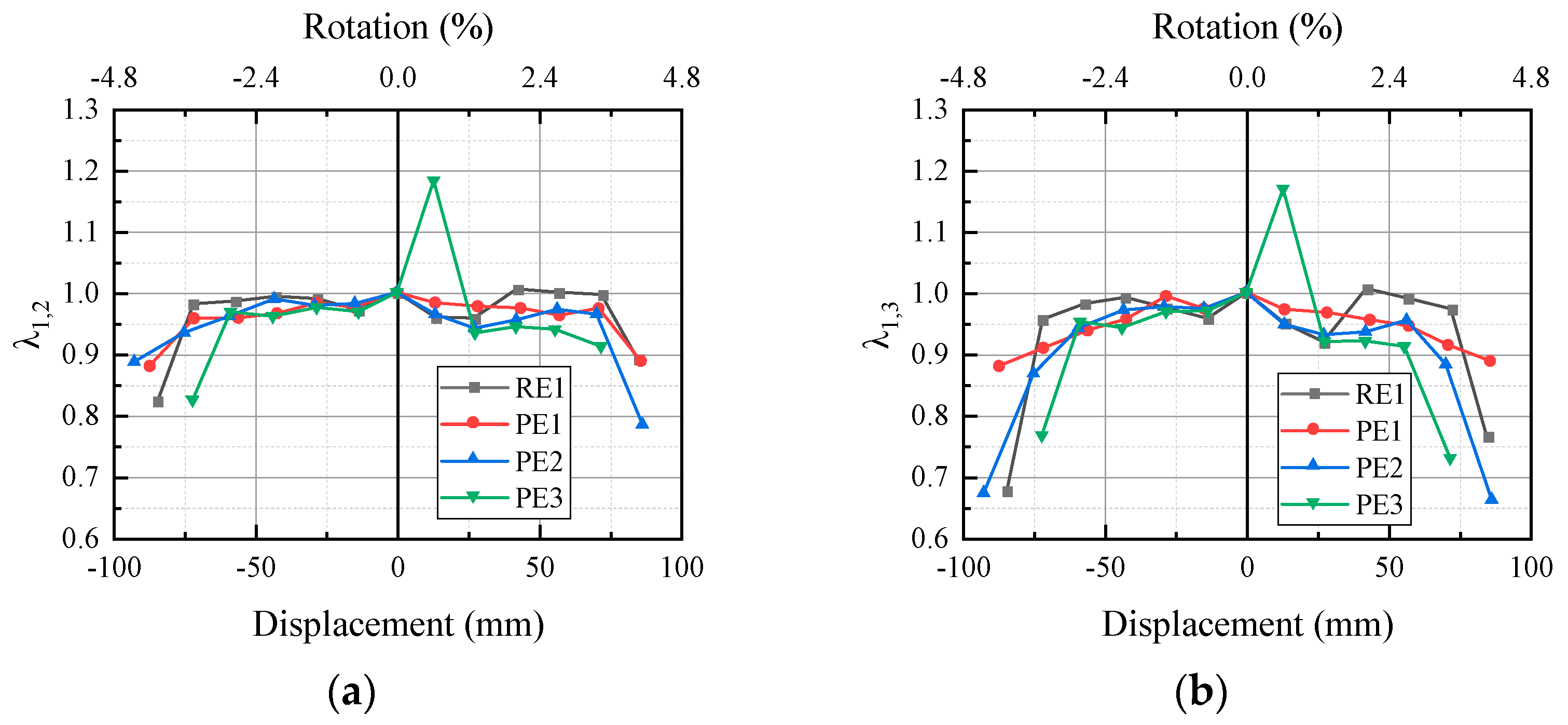
The strength degradation coefficient, λ, describes the strength degradation. The ratio of the second cycle’s bearing capacity peak to the first cycle’s at the same displacement is represented by λ1,2, and the third cycle at the same displacement is represented by λ1,3. Figure 14 illustrates the relationship between the strength degradation coefficients λ1,2 and λ1,3 of various specimens with the beam end displacement, as well as the ratio of the peak bearing capacity to the first cycle’s peak bearing capacity. It shows that before the displacement of 75 mm, except that PE3’s strength was not degraded and improved when the displacement was 15 mm, it was found through analyzing the test data that when PE3 was loaded at the 15 mm level, the first cycle was not loaded to the target displacement, and the second and third cycles were loaded to the target displacement. The λ1,2 of the PE1, PE2, and PE3s at other displacements varied between 0.9 and 1.0, which was very close to PE1 with only a slight strength degradation, indicating that the second cycle’s peak bearing capacity was similar to that of first cycle. The second cycle’s peak load capacity is essentially the same. Compared with λ1,2, λ1,3 decreases more with displacement, indicating that the specimens are damaged more seriously by the third cycle. The four curves’ development tendencies are essentially the same, suggesting that the axial compression ratio and anchoring technique in the joint’s core area have minimal impact on the strength deterioration.
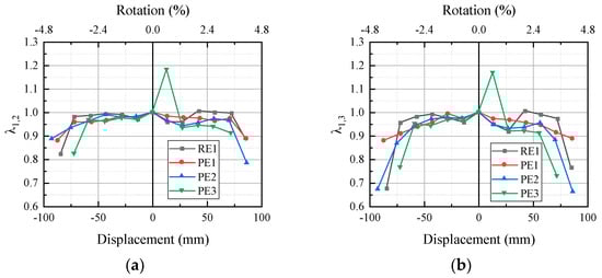
Figure 14.
Strength degradation. (a) λ1,2, (b) λ1,3,
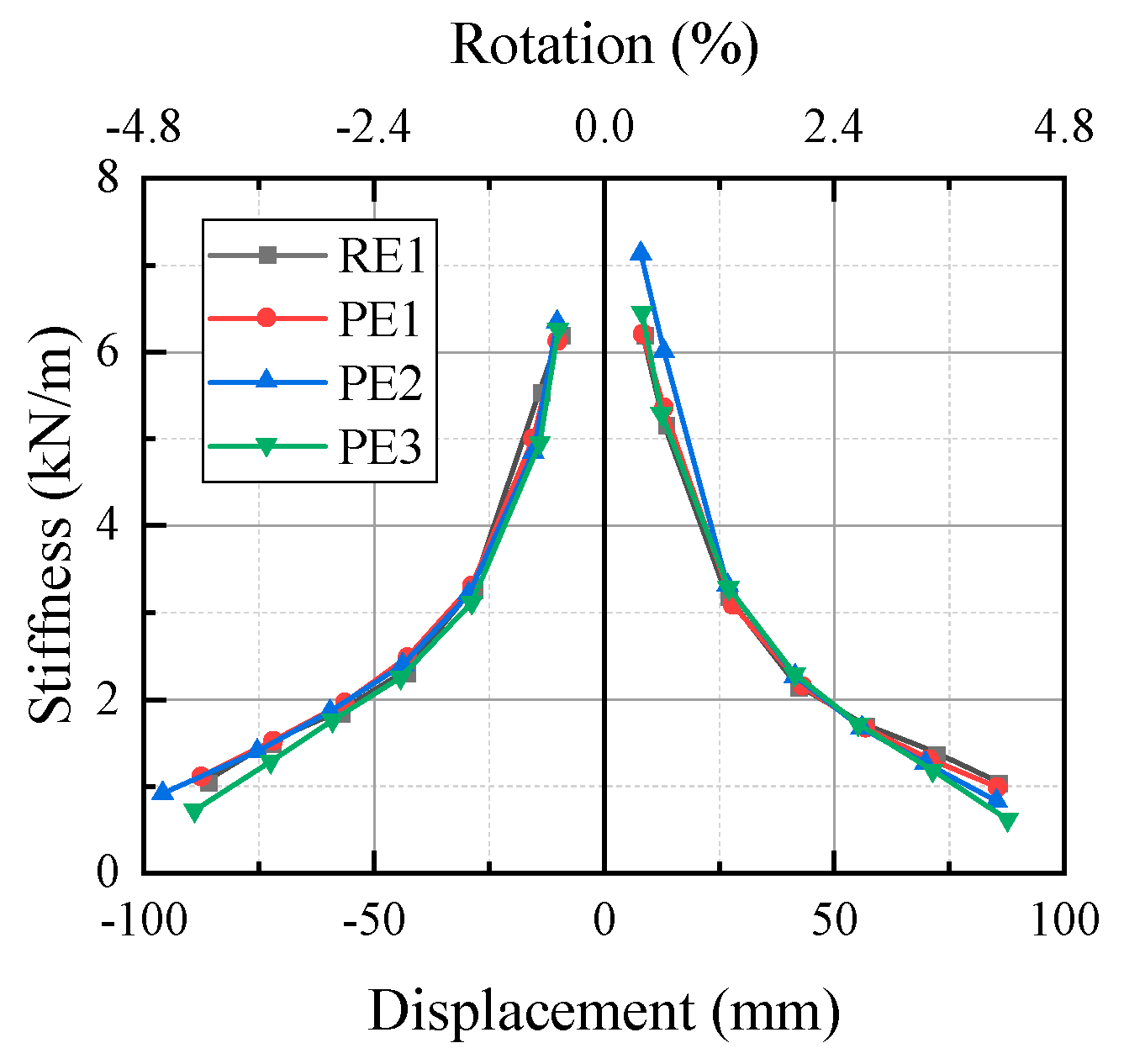
The structure’s overall stiffness is described by secant stiffness. The first cycle bearing capacity’s ratio of each load level to the corresponding displacement is K = F/Δ. Figure 15 illustrates the connection between the specimen stiffness K and the corresponding displacement Δ. On the whole, the forward stiffness of PE1, PE2, and PE3 was greater than the reverse stiffness, which was due to the asymmetrical arrangement of the beam’s upper and lower reinforcement. The beam of PE1 was symmetrically reinforced, and the forward stiffness was basically the same as the reverse stiffness. Compared with PE1, the initial stiffness and degradation trend of PE1 are basically the same. Compared with PE1, the forward initial stiffness of PE2 was 15.0% higher, the degradation trend in the early stage was slower, and the later stage was basically the same. The stiffness of the specimen has a great improvement effect. The forward and reverse initial stiffnesses of PE3 were 4.0% and 2.2% higher, respectively, than those of PE1. This suggests that the joint’s initial stiffness was not greatly improved by lengthening the beam longitudinal bars’ anchorage, and the degradation trend was essentially the same in the early stages. Reversed, the degeneration trend was more obvious.

Figure 15.
Stiffness degradation.
4.5. Specimens’ Seismic Performance Evaluation
The American standard ACI 374.1-05 specifies the seismic performance index of frame joints in high seismic intensity areas [47]. The four specimens’ seismic performance was further assessed in accordance with this specification, as indicated in Table 9, including three performance indicators: the residual strength ratio, the relative energy dissipation ratio, and the residual stiffness ratio. The peak load’s ratio in the third cyclic loading when the beam end rotation angle was 3.5% represents the residual strength ratio. The result shows that only the positive movement of PE3 was smaller than 0.75 (0.69). The ratio of the hysteresis loop area to the ideal elastic-plastic performance of the third cyclic loading when the beam end rotation angle was 3.5% represents the relative energy dissipation. The result shows that all the specimens were larger than the index of 0.125, and PE1, PE2, and PE3 were all better than RE1. The ratio of the secant stiffness to the initial stiffness when the third cyclic loading was between −0.35% and 0.35% when the beam end rotation angle was 3.5% represents the residual stiffness ratio. The result shows that all specimens were larger than the index of 0.05. Overall, except that the forward residual strength ratio of PE3 with torsional behavior was slightly lower than the standard index, all the specimens showed good seismic performance. The new joint can be used in structures with high seismic intensity areas and high seismic requirements.
Table 9.
Test results compared to the ACI 374.1-05 acceptance criteria.
4.6. Joint Shear Performance
The joint’s shear resistance must be studied in order to prevent the core area from shearing and to guarantee the frame structure’s adequate ductility. The joint’s shear deformation can be computed using Equation (3), where a and b stand for the joint’s height and breadth, which are taken to be constant throughout the test, c1 and d1 for the diagonal’s starting length, and c2 and d2 for the diagonal itself. In Figure 16, the distorted length is displayed [48].
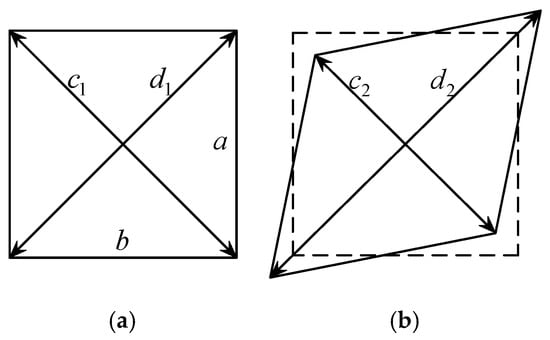
Figure 16.
Shear deformation of the joint zone. (a) Original. (b) Deformed.
The specification ACI 352R-02 [48] provides a method to calculate the shear stress in the joint’s core area, and the calculation formula is shown in Equation (4):
where, T and Vcol represent the beam top longitudinal reinforcement force and column end shear force, respectively, and hc and bj represent the joint’s height and effective width, respectively.
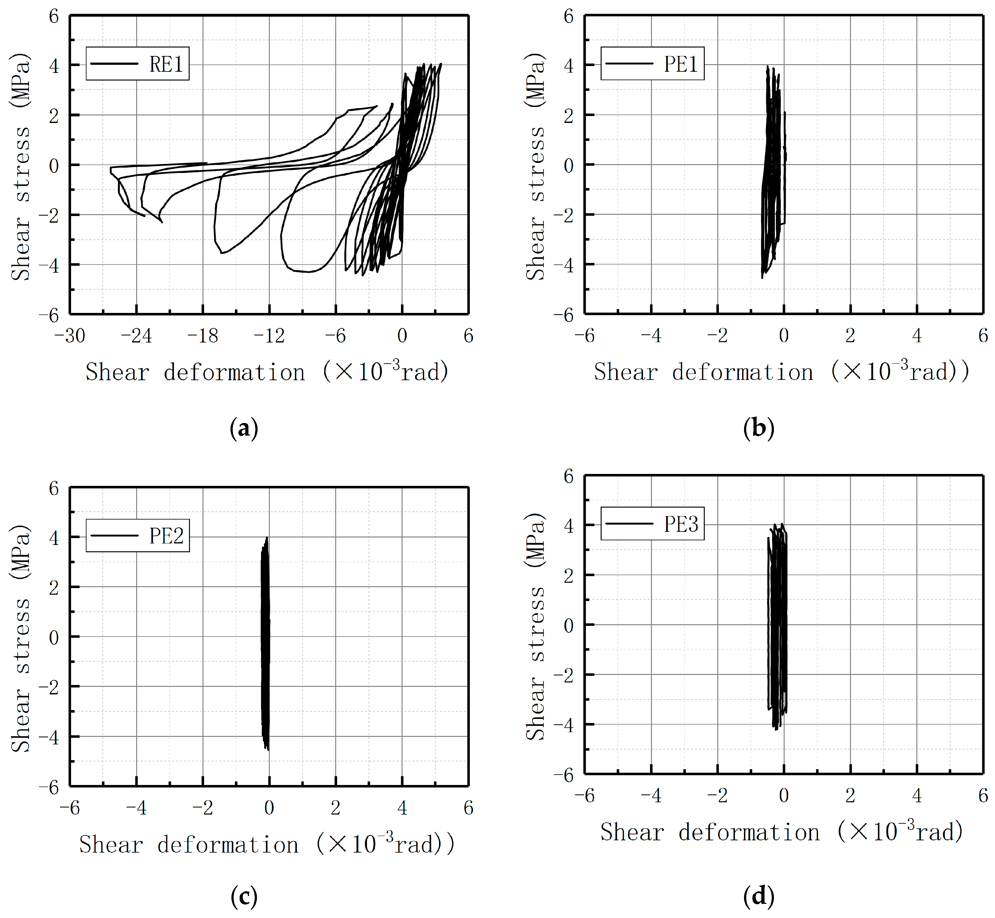
Through measured data, the shear stress-shear deformation hysteresis curve obtained using the above calculation method is shown in Figure 17. Table 10 lists the joint core area’s shear eigenvalues. Figure 17a,b indicate that RE1’s shear deformation increases continuously and exhibits a pinching phenomenon. Maximum shear stress in the core area was 4.43 MPa, and the maximum shear deformation reached 26.33 × 10⁻³ rad, while PE1’s curve was almost linear. When the maximum shear stress was 4.55 MPa, the maximum shear deformation was 0.67 × 10⁻³ rad, which was only 2.5% of that of RE1, and the maximum crack width in PE1’s core area was only 0.08 mm. It was much smaller than the 2.5 mm of RE1, and the damage degree of shear deformation to PE1 being significantly smaller than that of RE1, which indicates the new joint’s reliability fit into the “rigid joints” design requirement better. Compared with PE1, PE2 had an increased axial compression ratio, the two specimens’ maximum shear stress was consistent, the maximum shear deformation was reduced to 34.3% of PE1, and the maximum crack width was also reduced to 50.0% of PE1, indicating that an appropriate increase in the axial compression ratio is beneficial to the joint’s shear resistance. PE3’s maximum shear stress, maximum shear deformation, and maximum fracture width were all 7.3%, 28.4%, and 25.0% smaller than PE1’s, respectively, as a result of beam end torsion. In short, it can be seen from the four specimens’ shear hysteresis curves that compared to the cast-in-place joint, the new joints’ core area was in a low damage state and had a high shear redundancy. The new joints exhibited low shear deformation and high shear redundancy, with maximum shear deformation and crack width significantly lower than the cast-in-place joint.
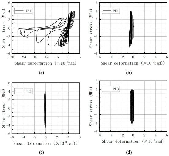
Figure 17.
Shear stress-shear deformation hysteretic loops. (a) RE1. (b) PE1. (c) PE2. (d) PE3.
Table 10.
Shear eigenvalue of the joint zone.
4.7. Anchorage and Lap Length Analysis
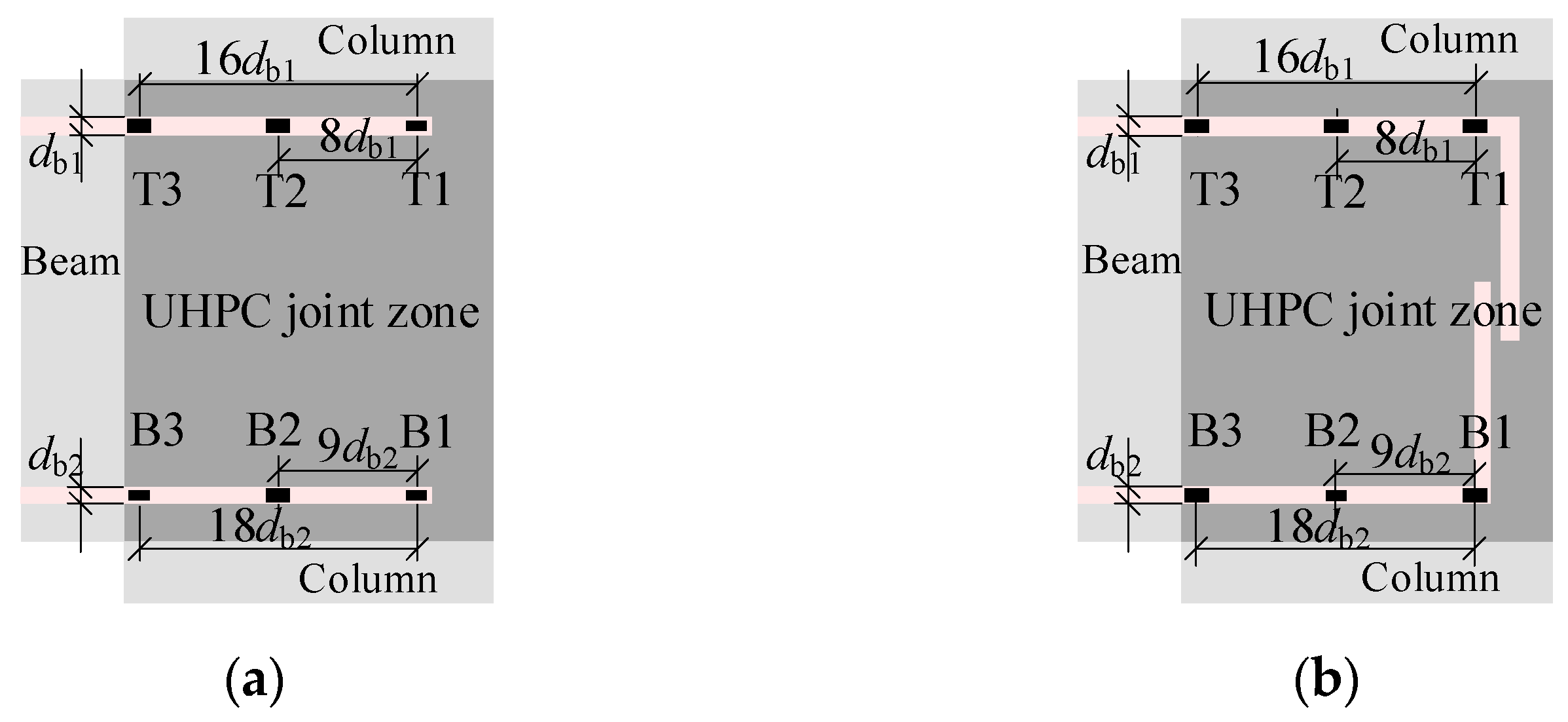
The steel bars and steel strands’ anchoring performance in the core area of joints is a key issue. Strain gauges are set at different positions of the steel bar to monitor the strain change. As seen in Figure 18, the top strain gauges are positioned at the joint core area’s edge (T3), the end of the steel bar (T1) (or at the bend), and the center of the two T2s, whereas T1 and T3 are both one decibel from the edge. The bottom strain gauge arrangement is the same as the top one.
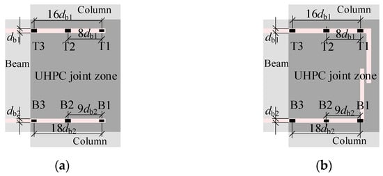
Figure 18.
Layout of strain gauges. (a) PE1 and PE2. (b) PE3.
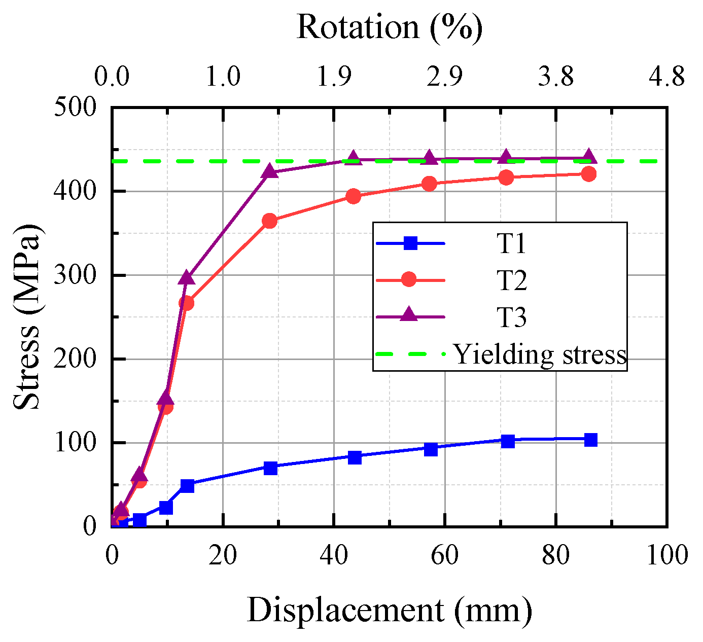
The constitutive model derived from the steel bar property test yielded a typical stress-displacement envelope curve of the longitudinal bar at the beam top by converting strain into the steel bar’s stress. Figure 19 indicates that T3 reached yield strength when the load was 45mm, and T2 did not reach the yield strength, but was very close to T3. Additionally, we found that T2 was only 8db from the end of T1 in Figure 18. The longitudinal reinforcement B2’s stress at the beam bottom achieved yield strength, as seen in Figure 20. Therefore, the maximum stress difference between T2 (B2) and T1 (B1) was used in this paper to calculate the bonding stress more accurately and make the calculation of the anchorage length more conservative.
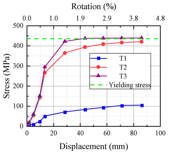
Figure 19.
The beam upper steel bars’ typical stress-displacement envelope curves.
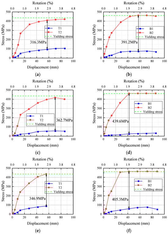
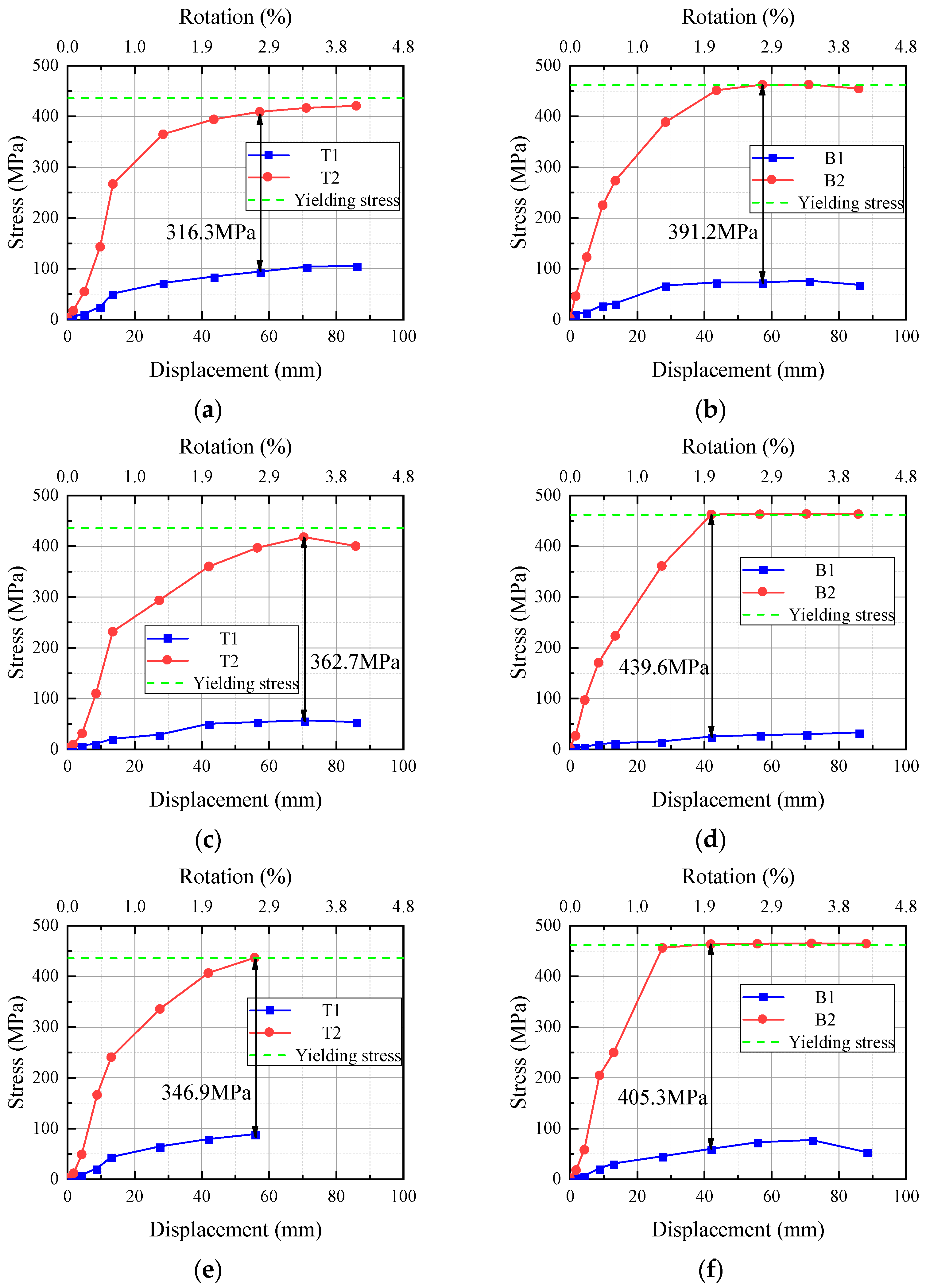
Figure 20.
Stress-displacement envelope curves of steel bars. (a) PE1 beam top. (b) PE1 beam bottom. (c) PE2 beam top. (d) PE3 beam bottom. (e) PE3 beam top. (f) PE3 beam bottom.
As shown in Figure 20e,f, the maximum stress difference between T2 (B2) and T1 (B1) of PE3s was very close to PE1’s, indicating that the use of steel bar straight anchors was sufficient to ensure the establishment of effective bond stress. Table 11 displays the average bonding stress of the beam longitudinal reinforcement, the maximum stress differential, and the distance between the T2 (B2) and T1 (B1) strain gauges of PE1 and PE2s. The beam’s longitudinal reinforcement was calculated using smaller bonding stress. The straight anchor’s lengths were 12db and 11.6db, and it is recommended to take 12db conservatively. It demonstrates that the beam longitudinal bars’ anchorage lengths can be lowered from 18db to 12db.
Table 11.
Anchorage length calculation.
Formula (5) provides the formula for designing longitudinal reinforcement anchorage length in Chinese Code [39], while Formula (6) provides the formula for determining the lap length:
where laE represents the anchorage length, ll represents the lap length, and ζa represents the anchorage length correction factor, which is taken as 1.0. ζaE represents the correction factor for the longitudinal tension steel bars’ anchorage length, which is taken as 1.05. ζl represents the correction factor of the longitudinal tension steel bars’ lap length, which is taken as 1.6. α represents the steel bar’s shape coefficient, which is 0.14 for the ribbed steel bar and 0.17 for the steel strand. d represents the steel bar’s diameter. fy represents steel bars’ yield strength. ft represents the UHPC’s axial tensile strength, calculated according to the formula [49]:
The longitudinal reinforcement’s calculated lengths at the beam top and bottom were 10.4db and 11.6db, respectively, and 12db was conservatively taken, which was the same as the test results’ analysis length.
For the steel strand’s anchorage length in the new joint’s core area, the standard calculation was 48db, and the test length of 40db did not have significant slippage, indicating that the bonding performance is reliable. According to Equation (6), the lap length of the column longitudinal bars was calculated to be 18db. In this study, the column longitudinal bars’ lap length was 16db, no slip phenomenon occurred, and the bonding performance was reliable. Strand anchorage lengths and rebar lap lengths are somewhat conservative.
5. Conclusions
In this paper, three PPCFEJ-UHPC new exterior joint specimens were subjected to low-cycle repeated load tests and compared with an equal-strength cast-in-place exterior joint specimen. The application of UHPC in the joint’s core area was studied, and the following conclusions can be drawn:
- (1)
- The cast-in-place exterior joint’s failure mode is the beam end yielding and then the joint shear failure. The new exterior joint’s failure mode is the beam end bending failure. In the later stage of the hysteresis curve, the former failure mode is coupled by significant pinching and inadequate energy dissipation capacity. The failure mode satisfies the design principle of “strong columns, weak beams, strong joints, and weak members” in order to guarantee the main structure’s safety.
- (2)
- The new joint’s bearing capacity is nearly identical to the cast-in-place joint (the former is 2.4% lower than the latter in the forward direction, and 2.7% higher in the reverse direction), which meets the requirements of the equivalent cast-in-place from the perspective of bearing capacity. The new joint’s energy dissipation performance is noticeably superior to that of the cast-in-place joint, as evidenced by the damping coefficient being at least 21.6% higher and the cumulative energy consumption being at least 21.7% higher. Each specimen has a ductility coefficient that is between 3.48 and 4.20, which is acceptable and marginally higher. The seismic structure designs required ductility coefficients of 3–4, which demonstrates that all of the test specimens have good ductility, and the new joint’s ductility coefficient is at least 6.1% higher than the cast-in-place joint specimen’s, indicating that the new joint performs better in terms of ductility than the old one. In summary, the new joint’s seismic performance is better than the cast-in-place joints. The evaluation in combination with the standards proposed in the ACI 374-05 specification also verifies that the new joint has very good seismic performance; The specimen’s bearing capacity remained basically unchanged, but the cumulative energy dissipation and ductility coefficient increased by 5.5% and 10.7%, respectively. It has been demonstrated that suitably raising the axial compression ratio can enhance the specimen’s seismic performance.
- (3)
- According to the anchorage length analysis, the recommended anchorage length for beam longitudinal bars is 12db, which is in line with the anchorage length computation in the Chinese code. This length can ensure the establishment of sufficient effective bond stress. Therefore, it is suggested to decrease the anchorage length of beam longitudinal bars from 18db to 12db. The anchoring length of beam steel strands 40db and the lap length of the column longitudinal bars 16db are lower than the calculated lengths of 48db and 18db in the specification, respectively. No significant slip occurred in this study, and the bonding performance is reliable. It shows that for this test specimen, the steel bar’s anchoring length calculation in UHPC is accurate in Chinese code, while the steel strand anchorage length and steel bar lap length calculation is a little conservative.
- (4)
- At the maximum shear stress level, the new joint’s core area has a maximum shear deformation of only 2.5% compared to the cast-in-place joint, and its maximum crack width is only 0.08 mm, significantly less than the cast-in-place joint’s 2.5 mm. The shear hysteresis curve is almost in an elastic state and has high shear redundancy. The experiment in this paper is conservative. In the future, an experimental study involving no stirrups in the joint’s core area would be meaningful.
- (5)
- Without steam curing, the UHPC’s mechanical properties can still reach sufficient strength, suggesting that standard curing techniques are also appropriate for UHPC and that its use in real building construction is, therefore, possible, but it is different from normal concrete. If the damage to the interface is serious, the interface can be chiseled, or the U-shaped steel bar can be set to enhance the integrity of the joint.
Author Contributions
Conceptualization, Z.W.; Methodology, Z.W.; Software, Z.W.; Validation, Z.W.; Formal analysis, Z.W.; Investigation, Z.W.; Resources, X.X., D.Z. and L.H.; Data curation, Z.W., J.L. and Y.X.; Writing—original draft, Z.W., J.L. and Y.X.; Writing—review & editing, X.X. and Z.W.; Visualization, Z.W.; Supervision, X.X.; Project administration, Z.W. and L.H.; Funding acquisition, X.X., D.Z. and L.H. All authors have read and agreed to the published version of the manuscript.
Funding
This research was funded by the Science and Technology Commission of Shanghai Municipality Project (20dz1202003), the Natural Science Foundation of China (52078364), and the Technology Innovation Project of Anhui (2020-YF21).
Data Availability Statement
No new data were created or analyzed in this study.
Conflicts of Interest
Author Dawei Zhang was employed by Shanghai Pudong Architectural Design & Research Institute Co., Ltd. Author Liang He was employed by China Construction Science & Technology Group East China Co., Ltd. The remaining authors declare that the research was conducted in the absence of any commercial or financial relationships that could be construed as a potential conflict of interest.
References
- Nicoletti, V.; Carbonari, S.; Gara, F. Nomograms for the pre-dimensioning of RC beam-column joints according to Eurocode 8. Structures 2022, 39, 958–973. [Google Scholar] [CrossRef]
- Fenwick, R. Comparison of recent New Zealand and United States seismic design provisions for reinforced concrete beam-column joints and test results for four units designed according to the New Zealand Code. Bull. N. Z. Natl. Soc. Earthq. Eng. 1984, 17, 69. [Google Scholar] [CrossRef]
- Kim, J.; Lafave, J.M. Joint Shear Behavior of Reinforced Concrete Beam-Column Connections Subjected to Seismic Lateral Loading; Department of Civil and Environmental Engineering, University of Illinois at Urbana—Champaign: Urbana, IL, USA, 2010. [Google Scholar]
- Pauletta, M.; Marco, C.D.; Frappa, G.; Miani, M.; Russo, G. Seismic behavior of exterior RC beam-column joints without code-specified ties in the joint core. Eng. Struct. 2020, 228, 111542. [Google Scholar] [CrossRef]
- Hakuto, S.; Park, R.; Tanaka, H. Seismic Load Tests on Interior and Exterior Beam-Column Joints with Substandard Reinforcing Details. ACI Struct. J. 2000, 97, 11–25. [Google Scholar]
- Parker, D.E.; Bullman, P.J.M. Shear strength within reinforced concrete beam-column joints. Struct. Eng. 1997, 75, 53–57. [Google Scholar]
- Zhou, Y.-J.; Wang, X.-T.; Sun, H.-R.; Chen, X.; Wang, T. Residual seismic performance for damaged RC frame based on beam-to-column joint subassemblies. Structures 2025, 71, 107980. [Google Scholar] [CrossRef]
- Blakeley, R.W.G.; Park, R. Seismic resistance of prestressed concrete beam-column assemblies. ACI Struct. J. 1971, 68, 677–692. [Google Scholar]
- Korkmaz, H.H.; Tankut, T. Performance of a precast concrete beam-to-beam connection subject to reversed cyclic loading. Eng. Struct. 2005, 27, 1392–1407. [Google Scholar] [CrossRef]
- Wilson, J.L.; Robinson, A.J.; Balendra, T. Performance of precast concrete load-bearing panel structures in regions of low to moderate seismicity. Eng. Struct. 2008, 30, 1831–1841. [Google Scholar] [CrossRef]
- Guan, D.; Guo, Z.; Xiao, Q.; Zheng, Y. Experimental study of a new beam-to-column connection for precast concrete frames under reversal cyclic loading. Adv. Struct. Eng. 2016, 19, 529–545. [Google Scholar] [CrossRef]
- Yee, A.; Eng, P. Social and environmental benefits of precast concrete technology. PCI J. 2001, 46, 14–19. [Google Scholar] [CrossRef]
- Yee, A.; Eng, P. Structural and economic benefits of precast/prestressed concrete construction. PCI J. 2001, 46, 34–43. [Google Scholar] [CrossRef]
- Yang, B.; Lü, X. Direct displacement-based aseismic design and application for prestressed precast concrete shear-wall structures. Eng. Mech. 2018, 35, 59–66, 75. (In Chinese) [Google Scholar]
- Chong, X.; Meng, S.-P.; Zhang, L.-Z. Numerical and theoretical analysis on seismic performance of post-tensioned prestressed concrete beam-column assemblages. Eng. Mech. 2013, 30, 153–159. (In Chinese) [Google Scholar]
- Wu, G.; Feng, D. Research progress on fundamental performance of precast concrete frame beam-to-column connections. J. Build. Struct. 2018, 39, 1–16. (In Chinese) [Google Scholar]
- Li, N.; Zhang, J.; Chu, X.; Liu, B. Experimental study on seismic behavior of pre-cast concrete beam-column sub-assemblage with cast-in-situ monolithic joint. Eng. Mech. 2009, 26, 41–44. (In Chinese) [Google Scholar]
- Xiong, X.-Y.; Xie, Y.-F.; Yao, G.-F. Study on shear behaviour of exterior reinforced concrete beam-column joints based on modified softened strut and tie model. Eng. Mech. 2022, 39, 55–71. (In Chinese) [Google Scholar]
- Hanson, N.W.; Conner, H.W. Seismic resistance of reinforced concrete beam-column joints. J. Struct. Div. 1967, 93, 533–559. [Google Scholar] [CrossRef]
- Tang, J.; Hu, C.; Yang, K.; Yan, Y. Seismic behavior and shear strength of framed joint using steel-fiber reinforced concrete. J. Struct. Eng. 1992, 118, 341–358. [Google Scholar]
- Ganesan, N.; Indira, P.V.; Sabeena, M.V. Behaviour of hybrid fibre reinforced concrete beam–column joints under reverse cyclic loads. Mater. Des. 2014, 54, 686–693. [Google Scholar] [CrossRef]
- Restrepo, J.I.; Park, R.; Buchanan, A.H. Design of Connections of Earthquake Resisting Precast Reinforced Concrete Perimeter Frames. PCI J. 1995, 40, 68–80. [Google Scholar] [CrossRef]
- Khan, M.I.; Al-Osta, M.A.; Ahmad, S.; Rahman, M.K. Seismic behavior of beam-column joints strengthened with ultra-high performance fiber reinforced concrete. Compos. Struct. 2018, 200, 103–119. [Google Scholar] [CrossRef]
- Zheng, Q.; Liu, Y.; Long, L.; Chen, G.; Ma, Y. Experimental research on seismic behavior of precast concrete frame connected with UHPC. Ind. Constr. 2019, 49, 85–91. (In Chinese) [Google Scholar]
- Maya, L.F.; Zanuy, C.; Albajar, L.; Lopez, C.; Portabella, J. Experimental assessment of connections for precast concrete frames using ultra high performance fibre reinforced concrete. Constr. Build. Mater. 2013, 48, 173–186. [Google Scholar] [CrossRef]
- Wang, Z.; Wang, J.; Liu, J.; Han, F.; Zhang, J. Large-scale quasi-static testing of precast bridge column with pocket connections using noncontact lap-spliced bars and UHPC grout. Bull. Earthq. Eng. 2019, 17, 5021–5044. [Google Scholar] [CrossRef]
- Zhang, Z.; Ding, R.; Nie, X.; Fan, J. Seismic performance of a novel interior precast concrete beam-column joint using ultra-high performance concrete. Eng. Struct. 2020, 222, 111145. [Google Scholar] [CrossRef]
- Ma, F.-D.; Deng, M.-K.; Yang, Y. Seismic experimental study on a uhpc precast monolithic concrete beam-column connection. Eng. Mech. 2021, 38, 90–102. (In Chinese) [Google Scholar]
- Yang, L.; Shi, C.; Wu, Z. Mitigation techniques for autogenous shrinkage of ultra-high-performance concrete—A review. Compos. Part B Eng. 2019, 178, 107456. [Google Scholar] [CrossRef]
- Sorelli, L.; Constantinides, G.; Ulm, F.; Toutlemonde, F. The nano-mechanical signature of Ultra High Performance Concrete by statistical nanoindentation techniques. Cem. Concr. Res. 2008, 38, 1447–1456. [Google Scholar] [CrossRef]
- Yuan, J.; Graybeal, B. Bond of reinforcement in ultra-high-performance concrete. ACI Struct. J. 2015, 112, 851. [Google Scholar] [CrossRef]
- Xiong, X.; Xie, Y.; Yao, G.; Liu, J.; Yan, L.; He, L. Experimental study on seismic performance of precast pretensioned prestressed concrete beam-column interior joints using uhpc for connection. Materials 2022, 15, 5791. [Google Scholar] [CrossRef]
- Xue, W.C.; Hu, X.Y.; Song, J.Z. Experimental study on seismic behavior of precast concrete beam-column joints using UHPC-based connections. Structures 2021, 34, 4867–4881. [Google Scholar] [CrossRef]
- Gao, X.; Xiang, D.; He, Y.; Li, J. Shear deformation and force transfer of exterior beam-column joints. ACI Struct. J. 2020, 117, 253–267. [Google Scholar]
- Saleem, M.A.; Mirmiran, A.; Xia, J.; Mackie, K. Development Length of High-Strength Steel Rebar in Ultrahigh Performance Concrete. J. Mater. Civ. Eng. 2013, 25, 991–998. [Google Scholar] [CrossRef]
- Xuan, S.; Zheng, H.; Liang, X. Research on anchorage length of steel strand embedded in ultra-high-performance concrete. Ind. Constr. 2020, 50, 114–118. (In Chinese) [Google Scholar]
- Maya, L.F.; Graybeal, B. Experimental study of strand splice connections in UHPC for continuous precast prestressed concrete bridges. Eng. Struct. 2017, 133, 81–90. [Google Scholar] [CrossRef]
- Ma, F.; Deng, M.; Fan, H.; Yang, Y.; Sun, H. Study on the lap-splice behavior of post-yield deformed steel bars in ultra high performance concrete. Constr. Build. Mater. 2020, 262, 120611. [Google Scholar] [CrossRef]
- GB 50010-2010; Code for Design of Concrete Structures. China Architecture & Building Press: Beijing, China, 2015. (In Chinese)
- GB/T 50081-2019; Standard for Test Methods of Concrete Physical and Mechanical Properties. China Architecture & Building Press: Beijing, China, 2019. (In Chinese)
- JGJ 369-2016; Code for Design of Prestressed Concrete Structures. China Architecture & Building Press: Beijing, China, 2016. (In Chinese)
- Park, R. Evaluation of ductility of structures and structural assemblages from laboratory testing. Bull. New Zealand Soc. Earthq. Eng. 1989, 22, 155–166. [Google Scholar] [CrossRef]
- Feng, P.; Qiang, H.-L.; Ye, L.-P. Discussion and definition on yield points of materials, members and structures. Eng. Mech. 2017, 34, 36–46. (In Chinese) [Google Scholar]
- Jiang, J.; Li, J.; Jin, W. Advanced Concrete Structure Theory; China Architecture & Building Press: Beijing, China, 2007. (In Chinese) [Google Scholar]
- Hu, B.; Kundu, T. Seismic performance of interior and exterior beam–column joints in recycled aggregate concrete frames. J. Struct. Eng. 2019, 145, 04018262. [Google Scholar] [CrossRef]
- GB 50011-2010; Code for Seismic Design of Buildings. China Architecture & Building Press: Beijing, China, 2016. (In Chinese)
- ACI 374.1-05; Acceptance Criteria for Moment Frames Based on Structural Testing and Commentary. American Concrete Institute: Farmington Hills, MI, USA, 2005.
- Joint ACI-ASCE Committee 352. Recommendations for Design of Beam-Column Connections in Monolithic Reinforced Concrete Structures. American Concrete Institute: Farmington Hills, MI, USA, 2002. [Google Scholar]
- Wang, J.; Hu, Y.; Liu, T.; Li, S.; Yin, H. Shear performance and bearing capacity calculation method for UHPC dry joints with large-keys. J. Build. Struct. 2021, 42, 177–185. (In Chinese) [Google Scholar]


Disclaimer/Publisher’s Note: The statements, opinions and data contained in all publications are solely those of the individual author(s) and contributor(s) and not of MDPI and/or the editor(s). MDPI and/or the editor(s) disclaim responsibility for any injury to people or property resulting from any ideas, methods, instructions or products referred to in the content. |
© 2025 by the authors. Licensee MDPI, Basel, Switzerland. This article is an open access article distributed under the terms and conditions of the Creative Commons Attribution (CC BY) license (https://creativecommons.org/licenses/by/4.0/).