Article

Planar Cross-Sectional Fitting of Structural Members to Numerical Simulation Results Obtained from Finite Element Models with Solid or Shell Elements

1
State Key Laboratory of Simulation and Regulation of Water Cycle in River Basin, China Institute of Water Resources and Hydropower Research, Beijing 100038, China
2
Key Laboratory of Engineering Materials of Ministry of Water Resources, China Institute of Water Resources and Hydropower Research, Beijing 100038, China
3
College of Civil Engineering and Architecture, Shandong University of Science and Technology, Qingdao 266590, China
4
Shandong Key Laboratory of Civil Engineering Disaster Prevention and Mitigation, Shandong University of Science and Technology, Qingdao 266590, China
5
School of Civil Engineering, Zhengzhou University, Zhengzhou 450001, China
*
Author to whom correspondence should be addressed.
Buildings 2025, 15(5), 797; https://doi.org/10.3390/buildings15050797
Submission received: 1 February 2025 / Revised: 24 February 2025 / Accepted: 26 February 2025 / Published: 28 February 2025
(This article belongs to the Section Building Structures)

Abstract

:
Modeling complex conditions involving extensive engineering structures with large numbers of beams and columns often requires a mixture of analytical modeling based on beam theory and numerical simulations involving finite element models composed of solid or shell elements. However, high levels of deformation in the planar configuration of cross-sections arising under extreme external loads, such as intensive earthquakes, explosions, and hurricanes, greatly complicates the task of fitting the numerical simulation results to the planar cross-sections required by beam theory. The present work addresses this issue by proposing a fitting method based on a least squares approximation method. The fitting problem is first transformed into a process of solving a cubic equation whose coefficients are integrals over the simulated cross-section. The solution of the cubic equation is defined using explicit formulae developed for calculating the integrals over the surfaces of single solid or shell elements lying within the cross-section by combining the shape functions and degree of freedom results of the elements. The proposed fitting method is then applied for analyzing the blast resistance of steel structures. The potential application of the proposed method is demonstrated by evaluating the rotations, shear deformations, and moment–curvature relationships of the fitted cross-sections.

1. Introduction

At present, many numerical simulation methods, such as the applied element method (AEM), the discrete element method (DEM), and the smoothed particle hydrodynamics method (SPH), are used for analysis of building structures [1,2,3]. Among all widely used numerical simulation methods, the finite element method (FEM) is a facile tool for studying the behaviors of engineering structures under arbitrary load configurations. For example, FEM models composed of refined solid or shell elements have facilitated the accurate modeling of complicated mechanical behaviors [4,5,6,7,8,9], such as those that develop in structural members, like beams and columns, under extreme external loads arising from intensive earthquakes, explosions, and hurricanes [10,11,12]. Here, concrete structural members are usually modeled with solid elements to facilitate the simulation of various characteristic failure mechanisms, such as cracks caused by tension stress [13], slips in steel reinforcement [14], and crushed compressed zones. In contrast, steel beams can suffer losses in the bearing capacity due to the local buckling of thin plates under principle compressive stresses [15] and tearing under tensional stresses [16]. Hence, both solid and shell elements have been applied to study the complicated failure processes of steel structural members [17,18]. Nonetheless, numerical simulations involving FEM models with refined elements require massive computational resources. As such, FEM simulations are often impractical for studying the behaviors of engineering structures with large numbers of beams and columns.
This issue is often addressed by applying beam theory, which is widely used for studying the behaviors of engineering structures composed of beams, columns, and trusses [19,20,21,22]. Two common modeling methodologies based on beam theory are classical Euler–Bernoulli beam theory (CBT) and Timoshenko beam theory (TBT) [23]. Here, CBT assumes that the cross-section remains perpendicular to the beam axis at all times. Hence, this theoretical framework cannot consider effects of shear deformation in cross-sections. In contrast, TBT can consider shear deformation by allowing the cross-section to deviate from the norm of the beam axis [24]. Although CBT and TBT treat shear deformations in different ways, they share the same key assumption of beam theory that the initially planar cross-section remains planar under beam loading.
As a result of the prominence of beam theory and its key assumption, many quantitative analyses and structural indices are based on the plane wherein the deformed cross-section lies. For example, the ductility of concrete beams and columns can be calculated via rotation capacity analysis by rotation of the normal vector of the critical cross-section plane at yield and collapse states [25]. Also, shear deformation in the cross-section plane can be approximated in TBT as the change in angle between the normal vector of the cross-section plane and the beam axis [24]. Furthermore, moment–curvature relationships are significant components facilitating the study of cross-section behaviors and constructing efficient beam element models [26]. To quantify moment–curvature relationships, the curvatures of cross-sections should be calculated. For scenarios involving beams developing large deflections and shear deformations, the curvature of each cross-section is calculated according to the derivative of rotation of the cross-section plane with respect to the arc length to obtain reasonable accuracy [27]. It is important to determine the cross-section plane and its rotation when applying beam theory.
Owing to the importance of the cross-section plane and its rotation in beam theory, it is important to apply numerical simulations based on solid or shell element models to determine the cross-section plane and then apply these results within beam theory. The determination of the cross-section plane mainly includes finding the center and normal vector of the plane by data-fitting to the results obtained from solid or shell element models. This is typically facilitated by meshing a structural member into several solid or shell elements. After meshing, there should be mesh nodes lying on the plane of each cross-section of interest before loading the FEM models. However, cross-sections that are initially planar when the member is meshed can potentially lose their planar configuration during simulation owing to high-order deformation [28] and variations in the shear strain over the cross-section [29]. This is particularly problematic under conditions of severe loads, such as for accidents caused by explosions of hazardous chemicals [30,31]. Here, high blast loads can cause steel structural members to undergo local buckling, large deformation, and large rotation (including bending flexure and distortion) [32,33,34]. The resulting high level of distortion in the planar configuration of the cross-section greatly complicates the task of fitting the deformed cross-section obtained by numerical simulation to a plane.
The present work addresses this issue by proposing a method to fit the distorted cross-section planes obtained by numerical simulation based on least squares approximation. The remainder of this paper is organized as follows. The proposed cross-section fitting method is presented in Section 2 along with the means of solving the corresponding cubic equation involving integrals of variables over element surfaces. Thus, explicit formulae are constructed in Section 3 to calculate the integrals of four-node shell elements and eight-node solid elements. The proposed fitting method is then validated in Section 4, followed by application for analyzing the blast resistance of steel structures, where the symmetrical mechanical behaviors of steel columns, shear deformation of tapered I-section columns, and the moment–curvature relationships of tapered I-section columns are evaluated under blast loads caused by high TNT-equivalent detonations. Finally, the report is concluded in Section 5.

2. Least Squares Approximation Fitting Method

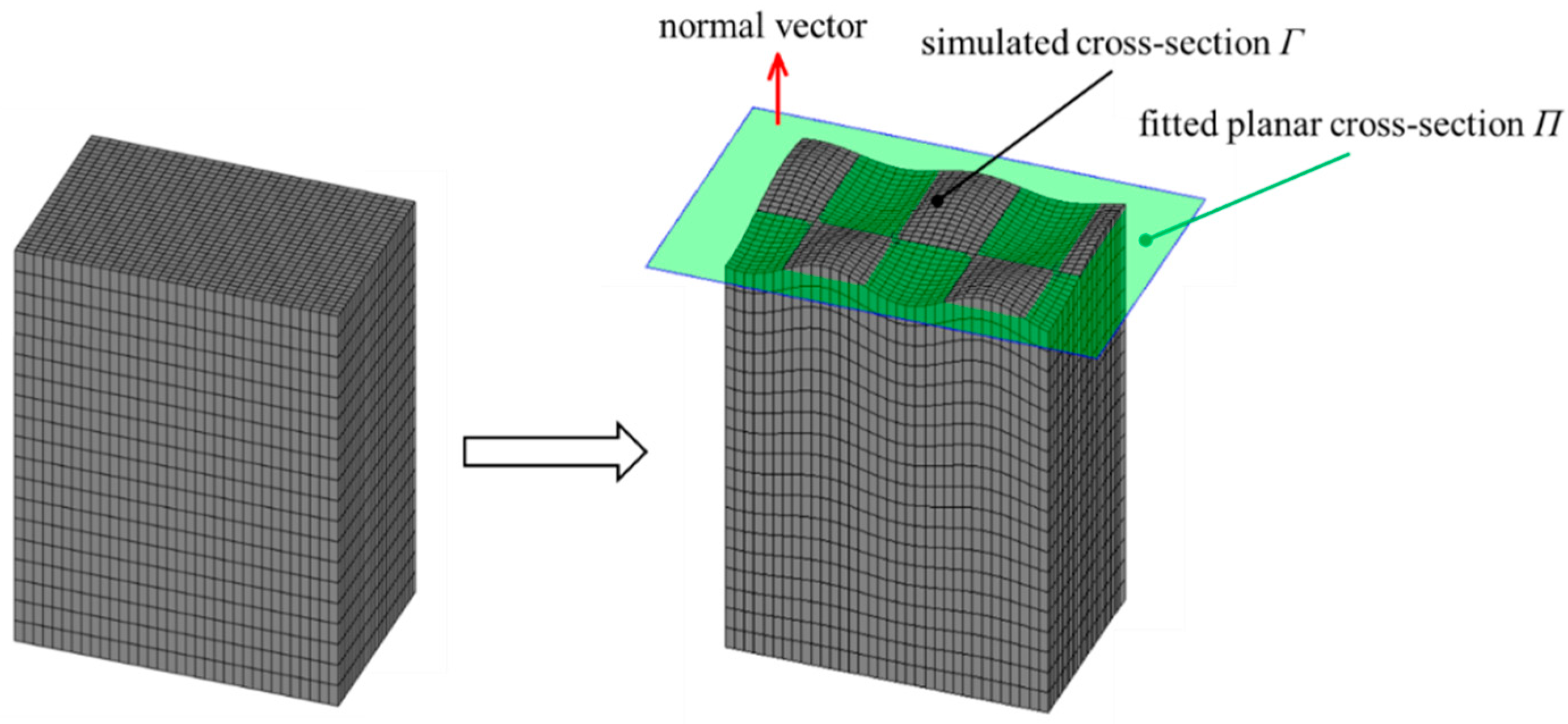
2.1. Equation for Fitting Planar Cross-Sections

The process of fitting a deformed cross-section obtained during numerical simulation of an FEM model to a perfect plane is illustrated in Figure 1. As can be seen, the elements of the FEM model are given in grey, the simulated surface is denoted as Γ, and the fitted planar surface is denoted as Π.
The planar surface Π is described mathematically, as follows:
A x + B y + C z + D = 0 ,
where (x, y, z) are the spatial coordinates of any point on the plane, and the coefficients A, B, C, and D are the unknown variables to be solved. The normal vector of Π given by the red arrow in Figure 1 is parallel to the spatial vector [A B C]T.
The deformed cross-section of interest Γ, which was initially planar prior to simulation, is the exterior boundary of all finite elements attached to the cross-section surface for both solid and shell element models. Let the coordinates of any point on the curved surface of Γ be denoted as (x0, y0, z0). We then define the distance from point (x0, y0, z0) to the fitted plane Π as:
d = A x 0 + B y 0 + C z 0 + D A 2 + B 2 + C 2
We further calculate the coordinate of the centroid point (xc, yc, zc) on the surface Γ, as follows:
x c = Γ x 0 d S Γ 1 d S y c = Γ y 0 d S Γ 1 d S z c = Γ z 0 d S Γ 1 d S
Although the domain is discretized into a multitude of subdomains in the FEM scheme, the meshed cross-sectional surface still represents a continuous surface, not just discrete nodes, because a continuous surface is associated with each element. Therefore, the distance, d, in Equation (2) is a continuous piecewise-smooth function of the argument (x0, y0, z0) operative over the piecewise-smooth domain of the simulated cross-section surface Γ. The principle of least squares approximation represents the determination of coefficients A, B, C, and D, providing the minimum value in the Euclidean norm of d, denoted as ‖d2. The value of ‖d2 can be obtained as the following surface integral over Γ with respect to the surface area, S:
d 2 = Γ d 2 d S
To obtain a more tractable form for the fitting process, we define a vector x = [A B C D]T and a function F = (‖d2)2. As such, the cross-section fitting problem based on least squares approximation can be succinctly denoted as:
min x F x
To solve this problem, we set the partial derivatives of F with respect to the coefficients of planar surface Π to zero, which yields the following:
F A = 0 F B = 0 F C = 0 F D = 0
Substituting Equations (2) and (4) into (6) and interchanging the integral and derivative operators yields the following expressions:
Γ 2 x 0 D + A x 0 + B y 0 + C z 0 A 2 + B 2 + C 2 2 A D + A x + B y + C z 2 A 2 + B 2 + C 2 2 d S = 0 Γ 2 y 0 D + A x 0 + B y 0 + C z 0 A 2 + B 2 + C 2 2 B D + A x 0 + B y 0 + C z 0 2 A 2 + B 2 + C 2 2 d S = 0 Γ 2 z 0 D + A x 0 + B y 0 + C z 0 A 2 + B 2 + C 2 2 C D + A x 0 + B y 0 + C z 0 2 A 2 + B 2 + C 2 2 d S = 0 Γ 2 D + 2 A x 0 + 2 B y 0 + 2 C z 0 A 2 + B 2 + C 2 d S = 0
Equation (7) can be rewritten as follows:
D Γ x 0 d S + A Γ x 0 2 d S + B Γ x 0 y 0 d S + C Γ x 0 z 0 d S = A Γ D + A x 0 + B y 0 + C z 0 2 d S A 2 + B 2 + C 2 D Γ y 0 d S + A Γ x 0 y 0 d S + B Γ y 0 2 d S + C Γ y 0 z 0 d S = B Γ D + A x 0 + B y 0 + C z 0 2 d S A 2 + B 2 + C 2 D Γ z 0 d S + A Γ x 0 z 0 d S + B Γ y 0 z 0 d S + C Γ z 0 2 d S = C Γ D + A x 0 + B y 0 + C z 0 2 d S A 2 + B 2 + C 2 D Γ 1 d S + A Γ x 0 d S + B Γ y 0 d S + C Γ z 0 d S = 0
Solving the last expression in Equation (8) yields the following expression for D:
D = A Γ x 0 d S + B Γ y 0 d S + C Γ z 0 d S Γ 1 d S
Comparing the solution in Equation (9) with Equation (3) indicates that the centroid of the deformed cross-section Γ is always on the fitted cross-section Π. Substituting Equation (9) into the first three expressions in Equation (8) yields the following solutions:
A Γ x 0 d S + B Γ y 0 d S + C Γ z 0 d S Γ 1 d S Γ x 0 d S + A Γ x 0 2 d S + B Γ x 0 y 0 d S + C Γ x 0 z 0 d S = A ϑ A Γ x 0 d S + B Γ y 0 d S + C Γ z 0 d S Γ 1 d S Γ y 0 d S + A Γ x 0 y 0 d S + B Γ y 0 2 d S + C Γ y 0 z 0 d S = B ϑ A Σ x 0 d S + B Σ y 0 d S + C Σ z 0 d S Γ 1 d S Γ z 0 d S + A Γ x 0 z 0 d S + B Γ y 0 z 0 d S + C Γ z 0 2 d S = C ϑ
Here, we define the variable ϑ as:
ϑ Γ D + A x 0 + B y 0 + C z 0 2 d S A 2 + B 2 + C 2
The fitting process is further simplified by rewriting Equation (10) as follows:
M Y = 0 ,
where the vector Y = [A B C]T, and M is the following coefficient matrix:
M = Γ x 0 d S 2 Γ 1 d S + Γ x 0 2 d S ϑ Γ x 0 y 0 d S Γ x 0 d S Γ y 0 d S Γ 1 d S Γ x 0 z 0 d S Γ x 0 d S Γ z 0 d S Γ 1 d S Γ x 0 y 0 d S Γ x 0 d S Γ y 0 d S Γ 1 d S Γ y 0 d S 2 Γ 1 d S + Γ y 0 2 d S ϑ Γ y 0 z 0 d S Γ y 0 d S Γ z 0 d S Γ 1 d S Γ x 0 z 0 d S Γ x 0 d S Γ z 0 d S Γ 1 d S Γ y 0 z 0 d S Γ y 0 d S Γ z 0 d S Γ 1 d S Γ z 0 d S 2 Γ 1 d S + Γ z 0 2 d S ϑ
As can be seen, the individual elements of M can be denoted as follows:
m 1 , 1 Γ x 0 d S 2 Γ 1 d S + Γ x 0 2 d S ϑ , m 1 , 2 Γ x 0 y 0 d S Γ x 0 d S Γ y 0 d S Γ 1 d S , m 1 , 3 Γ x 0 z 0 d S Γ x 0 d S Γ z 0 d S Γ 1 d S , m 2 , 2 Γ y 0 d S 2 Γ 1 d S + Γ y 0 2 d S ϑ , m 2 , 3 Γ y 0 z 0 d S Γ y 0 d S Γ z 0 d S Γ 1 d S , m 3 , 3 Γ z 0 d S 2 Γ 1 d S + Γ z 0 2 d S ϑ .
Therefore, M is more simply given as follows:
M = m 1 , 1 m 1 , 2 m 1 , 3 m 1 , 2 m 2 , 2 m 2 , 3 m 1 , 3 m 2 , 3 m 3 , 3
We also know that Y cannot be the zero vector 0 because the normal vector of cross-section Π is parallel to vector [A B C]T. Thus, the following relationship is satisfied:
M = m 3 , 3 m 1 , 2 2 + 2 m 1 , 2 m 1 , 3 m 2 , 3 m 2 , 2 m 1 , 3 2 m 1 , 1 m 2 , 3 2 + m 1 , 1 m 2 , 2 m 3 , 3 = 0
Finally, the fitting process is further streamlined by simplifying the terms in Equation (14), as follows:
ο 1 Γ x 0 d S 2 Γ 1 d S + Γ x 0 2 d S ο 2 Γ y 0 d S 2 Γ 1 d S + Γ y 0 2 d S ο 3 Σ z 0 d S 2 Γ 1 d S + Γ z 0 2 d S
As a result, Equation (16) can be rewritten in the following cubic form:
ϑ 3 + ο 1 + ο 2 + ο 3 ϑ 2 + m 1 , 2 2 + m 1 , 3 2 + m 2 , 3 2 ο 1 ο 2 ο 2 ο 3 ο 1 ο 3 ϑ + 2 m 1 , 2 m 1 , 3 m 2 , 3 m 1 , 2 2 ο 3 m 1 , 3 2 ο 2 m 2 , 3 2 ο 1 + ο 1 ο 2 ο 3 = 0
Because only coefficients A, B, and C are unknown, Equation (18) includes only one unknown variable, ϑ . Substituting the solution of Equation (18) into Equation (10) yields a homogeneous linear system of equations for which an infinite number of solutions (A, B, and C) exist. However, all the groups of (A, B, and C) share the same ratio among A, B, and C, leading to the same expression of Equation (1), corresponding to only 1 plane. Therefore, picking any one of the groups of (A, B, and C) is sufficient to determine the fitted plane.

2.2. Explicit Solution of the Cubic Determination Equation

Although Equation (18) can be solved by iterative algorithms, the far greater efficiency obtained when applying an explicit formula is essential to ensure that the proposed methodology is practical for use with the results of complicated dynamic numerical simulations. This issue is addressed by applying Shengjin’s formulae [35].
To this end, we define a group of general coefficients for Equation (18):
a 1 b ο 1 + ο 2 + ο 3 c m 1 , 2 2 + m 1 , 3 2 + m 2 , 3 2 ο 1 ο 2 ο 2 ο 3 ο 1 ο 3 d 2 m 1 , 2 m 1 , 3 m 2 , 3 m 1 , 2 2 ο 3 m 1 , 3 2 ο 2 m 2 , 3 2 ο 1 + ο 1 ο 2 ο 3
Then, we rewrite Equation (18) as:
a ϑ 3 + b ϑ 2 + c ϑ + d = 0
We further define the following variables:
A S b 2 3 a c B S b c 9 a d C S c 2 3 b d
The discriminant is then defined as:
Δ = B S 2 4 A S C S
The discriminant Δ in Equation (22) can now be applied to simplify the solution process because the solution of Equation (20) varies according to the sign of Δ. If Δ > 0, we define the terms Y1 = ASb + 3a(−BS + Δ1/2)/2 and Y2 = ASb + 3a(−BS − Δ1/2)/2, and the solution is given as follows:
ϑ 1 = b Y 1 3 + Y 2 3 3 a ϑ 2 , 3 = b + 1 2 Y 1 3 + Y 2 3 ± 3 2 Y 1 3 Y 2 3 i 3 a
If Δ = 0, we define a term K = BS/AS, and the solution is given as follows:
ϑ 1 = b a + K ϑ 2 = ϑ 3 = K 2
If Δ < 0, we define the term ψ = arcosT, where T = (2ASb − 3aBS)/(2AS3/2), and the solution is given as follows:
ϑ 1 = b 2 A S cos θ 3 3 a ϑ 2 , 3 = b + A S cos ψ 3 ± 3 sin ψ 3 3 a
When the number of real positive roots of the cubic equation (Equation (20)) is greater than 1, the minimum root is applied to determine the fitted plane by the solutions of Equation (10) and Equation (9). The null space of the coefficient matrix of a homogeneous linear system of equations is the solution set of the equations. Therefore, the solution of Equation (10) is calculated by the following expression:
A B C = ker M ,
where ker(M) returns the null space of matrix M.

3. Integration over the Deformed Cross-Section Surface

As discussed in Section 2, the proposed method must solve a cubic equation whose coefficients include surface integrals over the simulated surface Γ. The integrands of these surface integrals are all continuous piecewise-smooth functions of the coordinates of points on the deformed surface Γ. Thus, explicit formulae must be provided to calculate these integrals facilely according to the deformed surface obtained using different types of finite elements to ensure that the proposed methodology is practical for use with the results of complicated dynamic numerical simulations. This was obtained in the present work for two types of elements, including four-node finite-strain shell elements and eight-node solid elements. Here, eight-node solid elements are very commonly employed in the numerical simulation of engineering structures. Meanwhile, finite-strain shell elements are always used in numerical simulations involving structural members with complicated mechanical behaviors because small deformation theory is not applicable when structural members develop geometrical nonlinearity under intensive loading conditions [36].

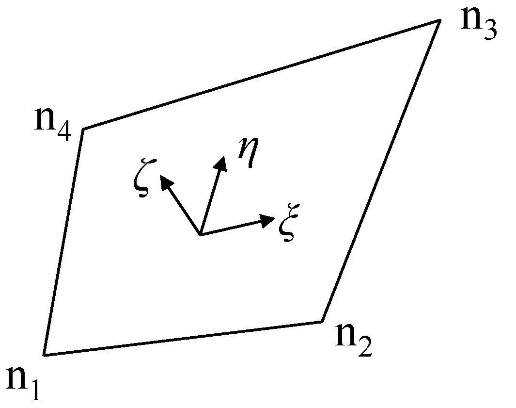
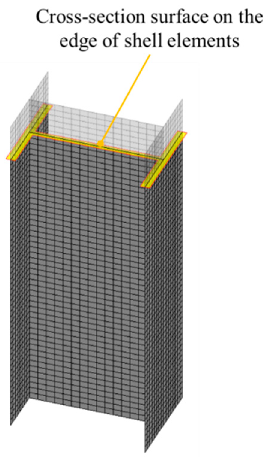
3.1. Integration of Four-Node Finite-Strain Shell Elements

The rotational degrees of freedom (DOFs) θx, θy, and θz defined under finite deformation differ from those defined under small deformation. Here, finite rotation defines θx, θy, and θz as elements of the axis vector Θ:
Θ = θ x θ y θ z
Meanwhile, the angle of rotation θ is given as the norm of the axis vector Θ:
θ = θ x 2 + θ y 2 + θ z 2 ,
and the axis of rotation is parallel to the axis vector Θ. Finally, the matrix corresponding to the rotation defined by the axis vector Θ is given as follows:
T = cos θ + 1 cos θ θ x 2 θ 2 1 cos θ θ x θ y θ 2 sin θ θ z θ 1 cos θ θ x θ z θ 2 + sin θ θ y θ 1 cos θ θ x θ y θ 2 + sin θ θ z θ cos θ + 1 cos θ θ y 2 θ 2 1 cos θ θ y θ z θ 2 sin θ θ x θ 1 cos θ θ x θ z θ 2 sin θ θ y θ 1 cos θ θ y θ z θ 2 + sin θ θ x θ cos θ + 1 cos θ θ z 2 θ 2
A local isoparametric coordinate system corresponding to a four-node shell element is illustrated in Figure 2, where local coordinate axes η and ξ lie within the shell element plane, and the local coordinate axis ζ is parallel to the thickness direction of the element. This model can now be employed to derive the following four shape functions of the shell element:
N 1 = 1 4 1 ξ 1 η N 2 = 1 4 1 + ξ 1 η N 3 = 1 4 1 + ξ 1 + η N 4 = 1 4 1 ξ 1 + η
The rotation matrix T and the shape functions can now be employed to calculate the global coordinate vector X for any point in a deformed element by interpolation:
x 0 , y 0 , z 0 T = X ξ , η , ζ = i = 1 4 N i X i + i = 1 4 N i h i ζ 2 T i e 3 0 ,
where Xi is the global coordinate vector of the i-th node ni, hi is the shell thickness at ni, which is usually the same at all nodes, and, if so, is denoted by h, Ti is the rotation matrix calculated by Equation (29) for ni, and e30 is the initial unit vector normal to the midpoint of the element surface prior to deformation.
For the structural member modeled with shell elements illustrated in Figure 3, we note that every cross-section consists of the edges of the shell elements attached to the cross-section.
The isoparametric coordinate of points on the shell element edge is ξ = ±1 or η = ±1, proven by the following equations taking the edge n1n2, where η equals −1 as an example. The global coordinate of any point n on the edge n1n2 is:
X = 1 2 1 ξ X 1 + 1 2 1 + ξ X 2 + 1 4 1 ξ h 1 ζ e 3 0 + 1 4 1 + ξ h 2 ζ e 3 0
The vector pointing from node n1 to n is:
n 1 n = X X 1 = 1 2 1 + ξ X 2 X 1 + 1 4 ζ 1 ξ h 1 + 1 + ξ h 2 e 3 0
The normal vector n of the surface represented by edge n1n2 of the shell element is determined as follows:
n = X 2 X 1 × e 3 0
The dot product between n and n 1 n can be given as follows:
n X X 2 = X 2 X 1 × e 3 0 1 2 1 + ξ X 2 X 1 + 1 4 ζ 1 ξ h 1 + 1 + ξ h 2 e 3 0 = 1 2 1 + ξ X 2 X 1 X 2 X 1 × e 3 0 + 1 4 ζ 1 ξ h 1 + 1 + ξ h 2 e 3 0 X 2 X 1 × e 3 0 = 0
The result of Equation (35) means the line connecting node n1 and point n is perpendicular to n. Since n is the normal vector of the surface represented by edge n1n2 and node n1 is on the surface, point n is also on the surface. Similar equations can be applied to prove that the isoparametric coordinate of points on the other three edges of a four-node shell element is ξ = ±1 or η = 1. Thus, the application of Equation (31) involves four circumstances where the isoparametric coordinate ξ = ±1 or η = ±1.
Combining the description of the cross-section in Figure 3 with the interpolation process given by Equation (31), we can define the surface integrals over the surface Γ in Equation (17) associated with the coefficients o1, o2, and o3 in Equation (18) using the form Γ f X d S . Since a cross-section consists of the edges of the shell elements attached to the cross-section, we can define the surface Γ as follows:
Γ = Γ e ,
where Γe is the edge surface of a given shell element. This yields the following relationship:
Γ f X d S = Γ e f X d S
Calculation of Equation (37) is demonstrated as following for the element edge n1n2 as an example, where η = −1. The surface differentiation is calculated as follows:
d S = X ξ , ζ ξ d ξ × X ξ , ζ ζ d ζ = 1 8 h X 2 X 1 × 1 ξ T 1 + 1 + ξ T 2 e 3 0 1 16 h 2 ζ 1 + ξ + 1 ξ T 1 e 3 0 × T 2 e 3 0 d ξ d ζ
The integrals in Equation (37) can be calculated through Gauss–Legendre quadrature, as follows:
Γ e f X d S 1 8 j = 0 m i = 0 n A j A i h X 2 X 1 × 1 ξ j T 1 + 1 + ξ j T 2 e 3 0 1 2 h 2 ζ i 1 + ξ j + 1 ξ j T 1 e 3 0 × T 2 e 3 0 f X ξ j , ζ i ,
where m and n denote the integration orders in the ξ and ζ directions, respectively, while the subscripts i and j correspond to the indices of quadrature points in the ξ-directional and ζ-directional discretizations, respectively.
The numerical integration defined in Equation (39) employs a total of nine Gauss quadrature points, utilizing a three-point Gauss quadrature scheme along each parametric direction, with m and n being 3. This configuration achieves fifth-order algebraic precision, exceeding the minimum requirement for full integration of four-node shell elements. Notably, as these integrals are employed solely for post-processing computed result data without intervening in the FEM solution algorithm, the selected quadrature scheme effectively avoids locking phenomena while maintaining computational accuracy. The specified integration order provides an optimal balance between numerical precision and computational efficiency for planar cross-sectional fitting. The positions and coefficients of the Gauss quadrature scheme are listed in Table 1.
In addition, the above analysis can assume that the normal vector is maintained perpendicular to the edge of the shell element because the shells applied in members assembling engineering structures, such as for steel plates, are usually not thick [37]. Therefore, Equation (37) can be approximated as:
Γ f X d S l e h 4 1 1 1 1 f X ξ , ζ d ζ d ξ ,
where le is the length of element edge n1n2. The coefficients o1, o2, and o3 in Equation (17) are obtained by explicitly writing all the integrals over Γe, which are summed over all elements in Equation (37), as follows:
Γ e 1 d S = l e h Γ e x 0 d S = l e h 2 x 1 + x 2 Γ e y 0 d S = l e h 2 y 1 + y 2 Γ e z 0 d S = l e h 2 z 1 + z 2
Γ e x 0 2 d S = l e h 3 36 3 e x 2 + 3 e x θ x 1 + 3 e x θ x 2 + θ x 1 2 + θ x 1 θ x 2 + θ x 2 2 + l e t 3 x 1 2 + x 1 x 2 + x 2 2 Γ e y 0 2 d S = l e h 3 36 3 e y 2 + 3 e y θ y 1 + 3 e y θ y 2 + s 1 y 2 + θ y 1 θ y 2 + θ y 2 2 + l e t 3 y 1 2 + y 1 y 2 + y 2 2 Γ e z 0 2 d S = l e h 3 36 3 e z 2 + 3 e z θ z 1 + 3 e z θ z 2 + θ z 1 2 + θ z 1 θ z 2 + θ z 2 2 + l e t 3 z 1 2 + z 1 z 2 + z 2 2
Γ e x 0 y 0 d S = l e h 3 72 6 e x e y + 3 e x θ y 1 + 3 e y θ x 1 + 3 e x θ y 2 + 3 e y θ x 2 + 2 θ x 1 θ y 1 + θ x 1 θ y 2 + θ x 2 θ y 1 + 2 θ x 2 θ y 2 + l e h 6 2 x 1 y 1 + x 1 y 2 + x 2 y 1 + 2 x 2 y 2 Γ e x 0 z 0 d S = l e h 3 72 6 e x e z + 3 e x θ z 1 + 3 e z θ x 1 + 3 e x θ z 2 + 3 e z θ x 2 + 2 θ x 1 θ z 1 + θ x 1 θ z 2 + θ x 2 θ z 1 + 2 θ x 2 θ z 2 + l e h 6 2 x 1 z 1 + x 1 z 2 + x 2 z 1 + 2 x 2 z 2 Γ e y 0 z 0 d S = l e h 3 72 6 e y e z + 3 e y θ z 1 + 3 e z θ y 1 + 3 e y θ z 2 + 3 e z θ y 2 + 2 θ y 1 θ z 1 + θ y 1 θ z 2 + θ y 2 θ z 1 + 2 θ y 2 θ z 2 + l e h 6 2 y 1 z 1 + y 1 z 2 + y 2 z 1 + 2 y 2 z 2
Here, the global coordinate system is applied to form the global coordinates of nodes n1 and n2 in the deformed geometry as (x1, y1, z1) and (x2, y2, z2), respectively, e30 is given as [ex ey ez]T, and the rotational DOFs of nodes n1 and n2 are given as (θx1, θy1, θz1) and (θx2, θy2, θz2), respectively. Explicit formulations for the remaining element edges are obtained similarly. It should be noted that Equations (40)–(43) are suitable for steel structures assembled with thin plates. For structures assembled with thick plates, the integrals over Γe should be calculated with Equation (39).

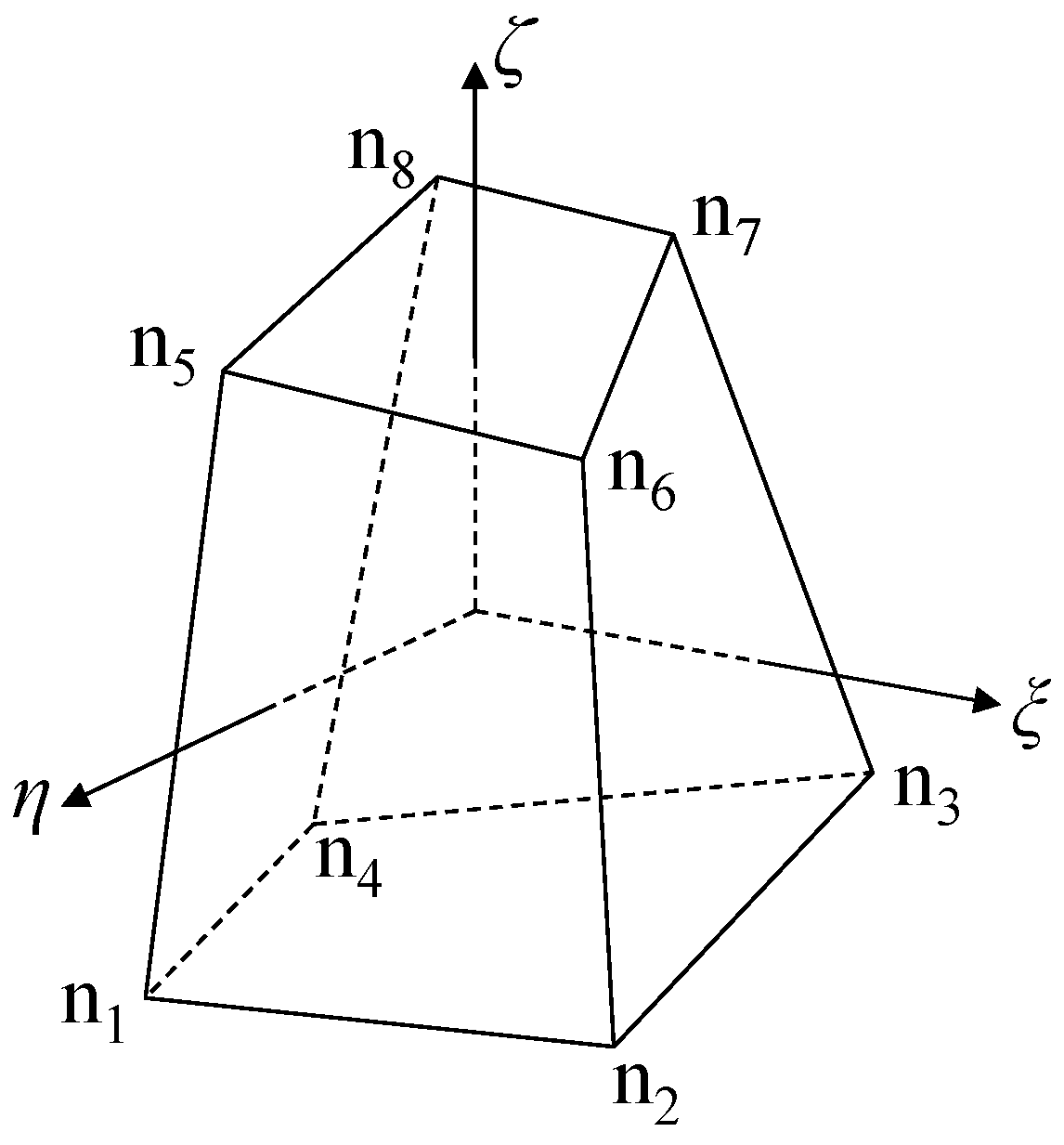
3.2. Integration of Eight-Node Solid Elements

A local isoparametric coordinate system corresponding to a typical eight-node solid element is illustrated in Figure 4. According to the discussion provided in Section 3.1, the shape functions of the element can be defined in isoparametric coordinates as:
N 1 = 1 8 1 ξ 1 η 1 ζ , N 2 = 1 8 1 + ξ 1 η 1 ζ , N 3 = 1 8 1 + ξ 1 + η 1 ζ , N 4 = 1 8 1 ξ 1 + η 1 ζ , N 5 = 1 8 1 ξ 1 η 1 + ζ , N 6 = 1 8 1 + ξ 1 η 1 + ζ , N 7 = 1 8 1 + ξ 1 + η 1 + ζ , N 8 = 1 8 1 ξ 1 + η 1 + ζ .
Moreover, the global coordinates of any point on the element are:
x 0 , y 0 , z 0 T = X ξ , η , ζ = i = 1 8 N i X i
Finally, as illustrated in Figure 1, we note that a cross-section would consist of the surfaces of the solid elements attached to the cross-section as well. Thus, Equation (37) can also be used to calculate integrals over the cross-sections of structural members modeled with solid elements.
The above analysis is demonstrated for element surface n1n2n3n4 as an example. Here, the element of surface integration for this subdomain of the cross-section is:
d S = X ξ d ξ × X η d η = 1 4 S 1 2 ξ , η + S 2 2 ξ , η + S 3 2 ξ , η d ξ d η ,
where the following vector variables have been applied:
S 1 ξ , η = η 1 x 1 x 2 + η + 1 x 3 x 4 ξ 1 y 1 y 4 ξ + 1 y 2 y 3 η 1 y 1 y 2 + η + 1 y 3 y 4 ξ 1 x 1 x 4 ξ + 1 x 2 x 3 S 2 ξ , η = η 1 x 1 x 2 + η + 1 x 3 x 4 ξ 1 z 1 z 4 ξ + 1 z 2 z 3 η 1 z 1 z 2 + η + 1 z 3 z 4 ξ 1 x 1 x 4 ξ + 1 x 2 x 3 S 3 ξ , η = η 1 y 1 y 2 + η + 1 y 3 y 4 ξ 1 z 1 z 4 ξ + 1 z 2 z 3 η 1 z 1 z 2 + η + 1 z 3 z 4 ξ 1 y 1 y 4 ξ + 1 y 2 y 3
Similar to integration of four-node shell elements, the integrals over surfaces of solid elements are calculated through Gauss–Legendre quadrature:
Γ e f X ξ , η d S 1 4 j = 0 m i = 0 n A j A i S 1 2 ξ j , η i + S 2 2 ξ j , η i + S 3 2 ξ j , η i f X ξ j , η i
The numerical integration scheme for solid elements, as presented in Equation (48), employs nine integration points, analogous to the shell element integration method detailed in Section 3.1. This configuration selects three integration points along each of the two directions. Notably, the number of integration points exceeds the requirement for full integration in eight-node solid elements. However, since this integration scheme is implemented in the post-processing phase, it avoids inducing finite element computational issues, such as element locking. The positions and coefficients of the Gauss quadrature scheme are the same as those listed in Table 1.
For circumstances where the cross-section is divided into fine meshes or mainly develops low-order deformation, the surfaces of solid elements on the cross-section experience little distortion. The numerical integration method with the one-point integration strategy is applied herein to calculate the integrals. To this end, we first define a parameter Sc, as follows:
S c = Γ e 1 d S = 1 2 y 1 z 2 y 2 z 1 y 1 z 4 + y 2 z 3 y 3 z 2 + y 4 z 1 + y 3 z 4 y 4 z 3 2 + x 2 z 1 z 2 x 1 + x 1 z 4 x 2 z 3 + x 3 z 2 x 4 z 1 x 3 z 4 + x 4 z 3 2 + x 1 y 2 x 2 y 1 x 1 y 4 + x 2 y 3 x 3 y 2 + x 4 y 1 + x 3 y 4 x 4 y 3 2
The explicit formulae employed to calculate integrals are given as follows:
Γ e x 0 d S = 1 4 S c x 1 + x 2 + x 3 + x 4 Γ e y 0 d S = 1 4 S c y 1 + y 2 + y 3 + y 4 Γ e z 0 d S = 1 4 S c z 1 + z 2 + z 3 + z 4
Γ e x 0 2 d S = 1 16 S c x 1 + x 2 + x 3 + x 4 2 Γ e y 0 2 d S = 1 16 S c y 1 + y 2 + y 3 + y 4 2 Γ e z 0 2 d S = 1 16 S c z 1 + z 2 + z 3 + z 4 2
Γ e x 0 y 0 d S = 1 16 S c x 1 + x 2 + x 3 + x 4 y 1 + y 2 + y 3 + y 4 Γ e x 0 z 0 d S = 1 16 S c x 1 + x 2 + x 3 + x 4 z 1 + z 2 + z 3 + z 4 Γ e y 0 z 0 d S = 1 16 S c y 1 + y 2 + y 3 + y 4 z 1 + z 2 + z 3 + z 4
Explicit formulations for the remaining element edges are obtained similarly.

4. Validation and Applications

The validity of the proposed methodology was initially confirmed through verification against theoretical solutions. Following this validation phase, the proposed method was applied for analyzing the blast resistance of steel structures, where the symmetrical mechanical behaviors of steel columns, shear deformation of tapered I-section columns, and the moment–curvature relationships of tapered I-section columns were evaluated under blast loads caused by high TNT-equivalent detonations.

4.1. Validation

This paper introduced a novel methodology for planar cross-sectional fitting of structural members to numerical simulation results derived from solid or shell FEM models. As the methodology was rigorously derived from fundamental FEM theoretical principles, its mathematical validity constitutes the primary verification focus. The consistency of fitting results with experimental data or physical measurements depends exclusively on the FEM model’s predictive accuracy, provided that the post-processing algorithm executes mathematically valid computations through rigorous adherence to derivation principles during operation. Furthermore, key output parameters, including spatial coordinates and orientation vectors of cross-sections, are inherently challenging to quantify experimentally. Consequently, the methodology’s validity was verified through comparative analysis with analytical solutions.
A finite element model utilizing shell elements was established to simulate the mechanical response of a doubly clamped I-beam under uniformly distributed load (UDL), as schematically represented in Figure 5. The numerical framework employed the coordinate system defined in the schematic, with the beam spanning 6.5 m (l) along the x-axis. The cross-sectional configuration comprised standard I-type dimensions: 300 mm vertical height and 220 mm horizontal flange width, with distinct thickness specifications—14 mm for the web and 18 mm for the flanges. The loading configuration applied a UDL of intensity q across the entire beam length. The structural component was fabricated from mild steel with a nominal yield strength of 235 MPa.
The analytical solution for a doubly clamped beam under UDL was formulated using Euler–Bernoulli beam theory, based on linear elastic material behavior and small deformation assumptions. Within this framework, the beam exhibited in-plane deformation only. Governing parameters of the cross-sectional fitting results were xc, zc, and A. Under small deformation conditions, the axial coordinate xc remained approximately constant, leaving zc and A as the dominant variables. These parameters were derived from the theoretical solution, as follows:
z c a = q x l x 2 24 E I A / N = q x l 2 3 l x + 2 x 2 12 E I ,
where EI denotes the elastic rigidity of the beam and N denotes the orientation vector of each cross-section and equals [A B C]T.
The maximum magnitude of the UDL was set to 20 kN/m to satisfy the linearity constraints of the theoretical framework. Figure 6 presents the corresponding deformation profile and von Mises stress distribution under this loading condition. Numerical results revealed a maximum stress of 52.7 MPa, which remained below the material’s yield threshold, while the deformation pattern demonstrated deflection magnitudes consistent with small-strain theory. These combined observations confirmed the validity of the linear elastic behavior assumption in both analytical and numerical approaches.
Figure 7 presents the comparative analysis of cross-sectional parameters derived from the proposed fitting method and corresponding theoretical solutions. These results were obtained under two distinct loading configurations: UDLs of q = 10 kN/m and q = 20 kN/m.
The transverse coordinate distribution (zc) of cross-sectional centroids exhibited symmetrical characteristics, while the orientation parameter distribution (A) demonstrated antisymmetric features. As shown in Figure 7a,b, both parameter distributions obtained through the proposed method showed congruence with theoretical solutions under the two loading conditions (q = 10 kN/m and q = 20 kN/m). By adopting theoretical solutions as reference benchmarks, the relative errors at distribution peaks were quantified. For the parameter xc, the relative errors under the two loading cases measured 0.25% and 0.26%, respectively. The relative error for parameter A converged to 5.59% under both loading conditions following numerical rounding procedures. The strong agreement between computational and theoretical results, combined with controlled relative errors, substantiated the validity of the proposed methodology for planar cross-sectional fitting.

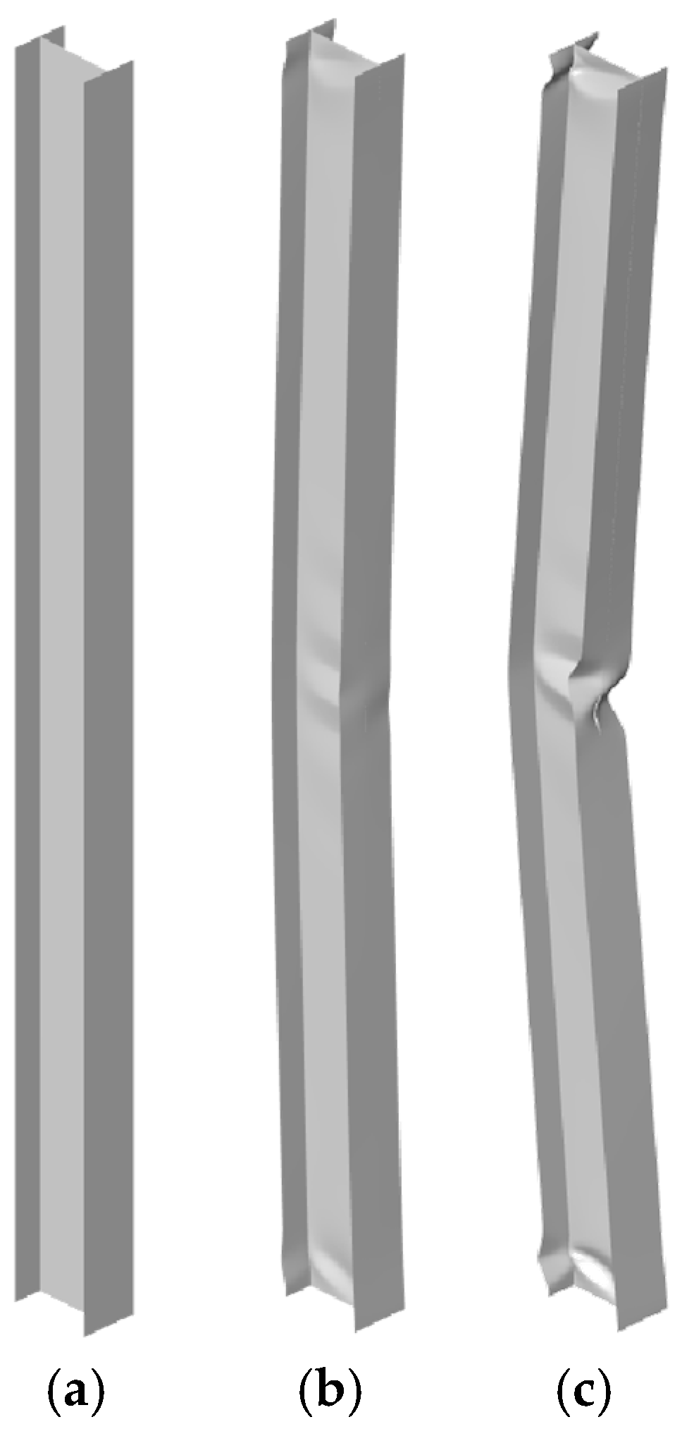
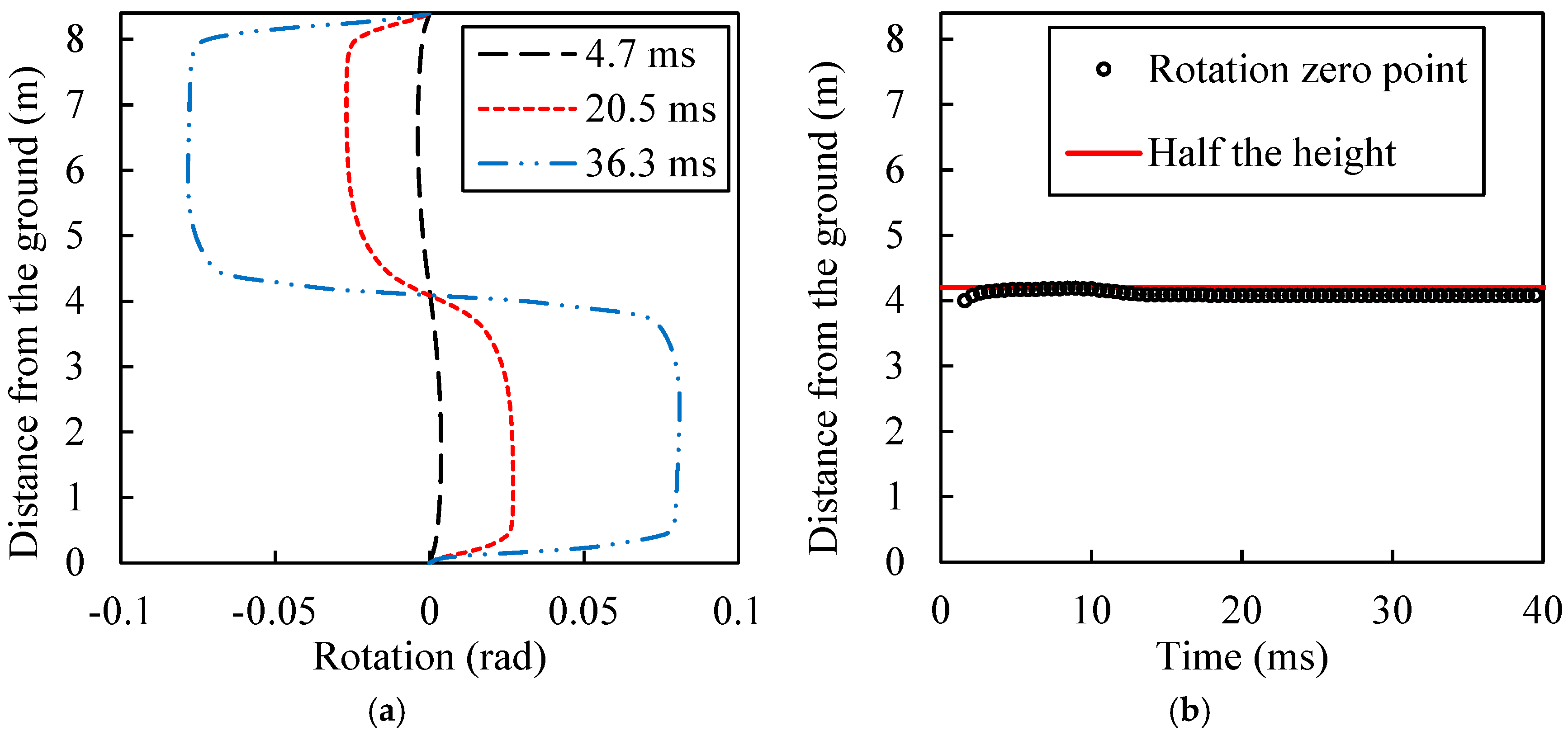
4.2. Symmetrical Mechanical Behavior of a Steel Column

The impingement of blast shock waves on walls of finite height and the clearing effects of walls are influential considerations when analyzing the resistance of steel structures to blast loads [38,39]. An accurate numerical approach was applied to simulate interactions between a target wall structure and a blast shock wave caused by the detonation of 500 t of TNT at a stand-off distance of 150 m from the target [40]. The clearing effects of the front wall are illustrated in Figure 8. As can be seen, the rarefaction wave response to the clearing effects propagated from the cornice to the bottom of the front wall. In addition, the overpressure at different points along the vertical direction of the front wall from the ground and the overpressure distribution on the front wall at different times are illustrated in Figure 9a,b, respectively. We note from Figure 9b that the blast load was not uniform over the front wall of the structure because of the propagation of the rarefaction.
The overpressure on the front wall illustrated in Figure 9 was applied to the front flange of an FEM model of a steel I-section column built with four-node finite-strain shell elements, and numerical simulations were conducted to calculate its dynamic response under the blast loads. The column had a height of 8.4 m, was fixed at both ends, and included a cross-section 600 mm high and 400 mm wide. The flange thickness was 26 mm, and the web thickness was 10 mm. The FEM model meshing included a mesh size of 20 mm, and all cross-sections of the column were planar prior to simulation. The deformations observed in the column under the blast load at 4.7 ms, 20.5 ms, and 36.3 ms are presented in Figure 10a–c, respectively.
As shown in Figure 10, the steel column developed large deformation and severe local buckling over the first 36 ms of simulation. The straight steel column had a fixed end and was symmetrical with respect to the plane lying on the middle of the column, which was the symmetry plane. The column behaved symmetrically if the applied external load was symmetrical, resulting in a symmetrical distribution of rotation with respect to height above the ground and a zero point of rotation at the middle of the column. However, the blast load applied on the column was not symmetrical, as indicated in Figure 9b, and the extent to which the column maintained symmetrical mechanical behavior must be evaluated. This was conducted herein by analyzing the extent of cross-section rotation.
As described in Section 2, the fitted cross-section was a plane whose normal vector was parallel to the vector N = [A B C]T. After applying Equations (23)–(26) and Equations (41)–(43), the rotation of a cross-section can be defined as:
θ = arcsin N × N 0 N ,
where N0 denotes the initial normal vector of the cross-section prior to simulation, which was [0 0 1]T for the column.
The rotations of all cross-sections of the FEM model were calculated at 4.7 ms, 20.5 ms, and 36.3 ms using Equation (54), and the obtained distributions in the rotation are presented in Figure 11a. The dashed lines in the figure indicate that the steel column engaged in symmetrical rotations at different times despite the non-symmetry of the blast load, as indicated by the overpressure distribution in Figure 9b. Hence, the steel column exhibited a zero point of rotation very close to the middle of the column (i.e., at 4.2 m). The distance of this zero point from the ground is plotted as a function of time in Figure 11b, along with a line representing the middle-point of the column. As can be seen, the zero point of the rotation distribution maintained a position at around 4.1 m from the ground, which is a little less than half the height of the column. Therefore, it can be concluded that the steel column can be treated as a symmetrical member under the applied blast load.

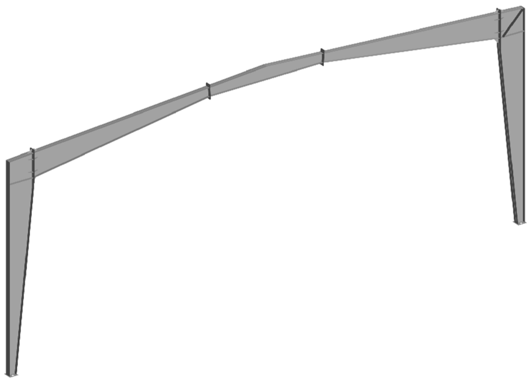
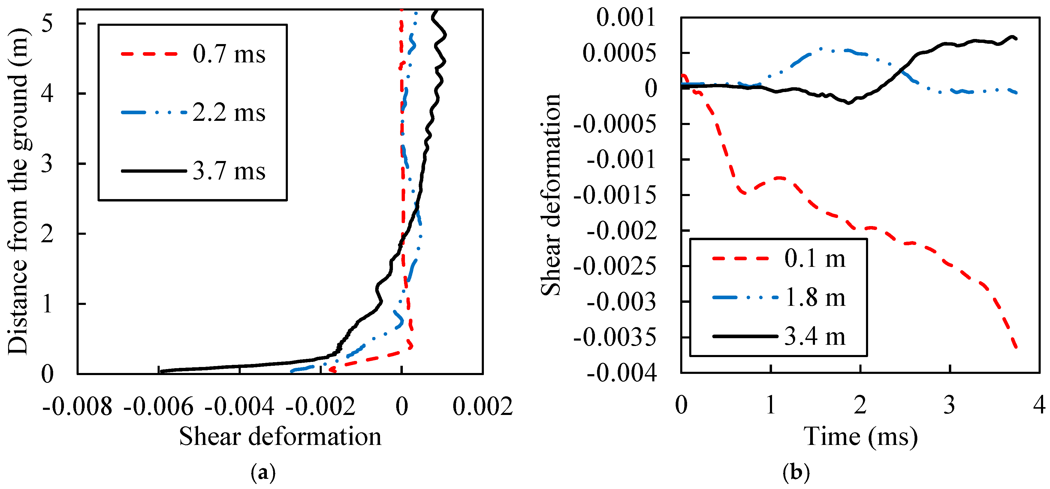
4.3. Shear Deformation of a Tapered I-Section Column

The dynamic response and performance of a portal frame, like that illustrated in Figure 12, under blast loads is of great importance because this a typical light-weight steel structure that is often used in factories and warehouses. The FEM model built with shell elements is illustrated in Figure 12, where the portal frame was formed of I-section structural members. The span of the frame was 18.0 m, and the maximum height of the frame was 6.9 m. As can be seen, the structural members of the portal frame were tapered, as is usually the case, and this complicated an analysis of the dynamic response of the frame under blast loads. The present work evaluated the blast performance of the frame under a blast wave propagating first to the front of the frame. Therefore, we can expect that the shear strain of the front column would greatly influence the dynamic response of the frame under the frame geometry considered. Thus, we evaluated the shear deformation of the front column of the portal frame under a blast load caused by the detonation of 200 t of TNT located 447 m away from the front of the portal frame.
As discussed, TBT assumes that the cross-section of the member remains planar after deformation. Therefore, we took the effects of shear strain into consideration by introducing a shear deformation value γ, as illustrated in Figure 13. According to the figure, the shear deformation γ is calculated as:
γ = φ θ ,
where the rotation of the cross-section θ can be calculated using Equation (54) and φ denotes the rotation of the beam axis. The value of φ can be calculated numerically for cross-sections of FEM models after numerical simulations, as follows:
φ = arcsin C k t C k + 1 t × C k 0 C k + 1 0 C k t C k + 1 t C k 0 C k + 1 0 ,
where C refers to centroid point of the cross-section, the superscripts refer to the time step when the centroid is calculated, and the subscripts refer to the successive ID numbers of the cross-sections.
Application of the 200 t TNT blast load to the FEM model of the portal frame yielded the shear deformation results for the front column shown in Figure 14, including the spatial shear deformation distributions at different numerical simulation times (Figure 14a) and the time histories of shear deformation at different cross-sections along the vertical direction of the column from the ground (Figure 14a). From curves in Figure 14, we can conclude that the shear deformation at the bottom of the column was greater than that observed for all other cross-sections. This was caused mainly by the comparably large shear force on the transversely fixed bottom cross-section, and because the bottom cross-section had the smallest shear rigidity of all cross-sections in the tapered column owing to its smaller cross-sectional area.

4.4. Moment–Curvature Relationship of a Tapered I-Section Column

The bending behavior of structural members also had a profound impact of their performance under lateral loads, like blast loads. Specifically, this was evaluated according to the moment–curvature relationship, which represents the bending rigidity EI of a member at different phases of flexural deformation, where the EI is defined as a function of the curvature ϕ (i.e., EI(ϕ)).
As was illustrated in Figure 13, a planar cross-section was not perpendicular to the axis of the beam under shear deformation. As such, the rotation of the cross-section was not equal to the derivative of the flexural displacement of the beam axis. Therefore, the curvature of any cross-section of the beam cannot be calculated based on the rotation of the beam axis, but should be calculated based on the rotation of the cross-section, as follows:
ϕ = d θ d s ,
where ds is the arc length of an infinitesimal segment of the beam axis, as shown in Figure 15.
The value of ϕ can be calculated numerically for the k-th cross-section of an FEM model at time t of a numerical simulation, as follows:
ϕ k , t θ k + 1 t θ k t C k t C k + 1 t
where the rotation θ of the different cross-sections at different times can be calculated using Equation (54). In addition, the moment of a cross-section can be obtained by calculating the integral of the axial stress multiplied by the plate thickness and distance from the cross-section centroid. The domain of the integral is over the cross-section surface Γ.
The moment–curvature relationships obtained for the tapered I-section column illustrated in Figure 16a were evaluated at the given cross-sections under a blast load caused by the detonation of 200 t of TNT at a stand-off distance of 447 m after 6.2 ms of simulation, and the results are presented in Figure 16b.
As shown in Figure 16b, the initial rigidity of the cross-section varied with its distance from the ground at the bottom of the tapered column because the width of the web of the tapered I-section column increased with increasing distance from the ground, and the rigidity of the cross-section correspondingly increased. We further note that the moment–curvature plots obtained for cross-sections located at 410 mm and 3410 mm were linear, while that observed for the cross-section at 1750 mm developed nonlinearly, indicating that the rigidity of this cross-section decreased owing to the yielding of the steel material under the blast load. Hence, this position represented a critical cross-section.
The later deformation observed for the critical cross-section located at 1750 mm under the blast load after 15.0 ms of simulation is illustrated in Figure 17a, where we note that the steel plate developed severe local buckling because of an increasing principal compression stress. The moment–curvature relationship observed for this critical cross-section is plotted in Figure 17b. As can be seen, the moment attained a peak value with increasing curvature and then decreased with a further increase in the curvature. The peak moment was an index of the bearing capacity of the critical cross-section. In addition, the negative correlation between moment and curvature showed that the rigidity turned negative after the peak, indicating that the cross-section lacked bearing capacity against bending deformation, which was demonstrated by the local buckling failure observed in Figure 17a.

5. Discussion

This study developed a cross-sectional fitting methodology to reconcile continuum finite element results (derived from shell/solid element discretizations) with beam-theoretical planar section requirements. The formulated framework demonstrated applicability to slender structural members—including beams, columns, and truss elements—whose mechanical behavior is governed by beam theory due to their slenderness ratios (longitudinal dimension significantly exceeding transverse dimensions). Illustrative cross-sectional schematics throughout this paper systematically elucidated the planar fitting protocol and its implementation. Crucially, the methodology retained validity for members with complex sectional geometries through decomposition into standard four-node shell or eight-node hexahedral element meshes, thereby extending its utility to composite building systems, such as moment frames, space trusses, and lattice structures. Notably, the present formulation excluded non-beam-type configurations, including joint connections, thin-shell structures (e.g., nuclear containment vessels), and massive block assemblies (e.g., hydroelectric spiral casings), where beam kinematic assumptions became fundamentally inadequate.
The section of application, Section 4, primarily served to illustrate the potential applicability of the proposed cross-sectional fitting method through a case study of steel structures under blast loading. It should be emphasized that the methodology demonstrated equal effectiveness for concrete structures and other types of external loads when appropriately adapted. The key distinction lies in the coefficient determination process: while Equations (40)–(43) were specifically developed for steel members, their concrete counterparts required substitution with Equations (48)–(52) for calculating the parameters in the fundamental Equation (18).
An explicit solution for cross-sectional fitting was established. To the best of the authors’ knowledge, this constitutes the first systematic cross-sectional fitting method. While computational efficiency comparisons with conventional approaches remain to be systematically investigated, the analytical nature of the proposed method, relying solely on explicit algebraic operations, suggests inherent computational advantages. The proposed method demonstrated its feasibility for large-scale models as a post-processing technique, independent of the FEM solution procedure, provided that the FEM computation has been successfully completed. The computational efficiency of the algorithm is primarily determined by two key factors: the number of cross-sections requiring fitting and the quantity of elements associated with each cross-section. Specifically, both an increase in the number of cross-sections to be processed and a larger number of elements connected to each cross-section will result in a greater computational processing time.
Notably, the proposed algorithm operated as a post-processing module that processed pre-computed FEM results (e.g., nodal displacements from shell/solid element analyses) to derive beam-relevant quantities (e.g., cross-sectional rotations and curvatures). This distinct implementation strategy decoupled the fitting process from the finite element solver, enabling direct application to standard FEM software outputs through their native post-processors. The methodological innovation lies in bridging continuum mechanics solutions with beam theory applications through cross-sectional fitting. This innovative approach not only facilitated beam theory interpretation of complex structural behavior but also enabled constructing efficient beam models of building structures.

6. Conclusions

The present work addressed the substantial challenge of fitting the results of numerical simulations involving FEM models with solid and shell elements to the planar cross-sections required by beam theory under the high levels of deformation arising under extreme external loads, such as intensive earthquakes, explosions, and hurricanes, by proposing a cross-section fitting method based on least squares approximation. The fitting problem was transformed into a process of solving a cubic equation whose coefficients were integrals over the simulated cross-section surfaces of the FEM model. High computational efficiency was obtained by solving the cubic equation explicitly based on the shape functions of the elements, in addition to the rotational DOFs of the nodes. The rotational DOFs in finite deformation problems were the elements of the vector quantifying the rotation. The integrals over solid model elements included changes in the area caused by distortion under applied loads and were calculated with a one-point integration strategy. While the cross-section fitting method proposed in this paper can be applied in many fields of structural analysis, the present work specifically applied the method for analyzing the blast resistance of steel structures. The results demonstrated that the proposed method was capable of obtaining the rotations, shear deformations, and moment–curvature relationships of cross-sections of steel columns. The distribution of rotations observed for vertical I-section columns fixed at both ends demonstrated that the column vibrated symmetrically despite the asymmetrical distribution of the applied overpressure. The shear deformation of the cross-section of a vertical tapered I-section beam near the bottom was observed to increase faster than other cross-sections. The moment–curvature relationships obtained for the cross-sections of a vertical tapered I-section beam demonstrated that the initial rigidity of the cross-sections varied according to their height above the ground. Also, the moment–curvature curve of the critical cross-section underwent degradation after the peak moment because of local buckling, which induced failure in the steel column.

Author Contributions

Conceptualization, X.Z., S.X. and F.S.; methodology, X.Z., S.X. and H.L.; software, X.Z., H.L. and M.L.; validation, X.Z., S.X. and H.L.; formal analysis, X.Z., S.X., H.L. and M.L.; investigation, X.Z., S.X., H.L. and F.S.; resources, X.Z., E.-F.D. and M.L.; data curation, X.Z.; writing—original draft preparation, X.Z., H.L. and F.S.; writing—review and editing, F.S. and E.-F.D.; visualization, M.L.; supervision, S.X.; project administration, M.L.; funding acquisition, X.Z., S.X. and F.S. All authors have read and agreed to the published version of the manuscript.

Funding

This research was funded by National Natural Science Foundation of China grant number 52408568; Open Research Fund of Shandong Key Laboratory of Civil Engineering Disaster Prevention and Mitigation, Shandong University of Science and Technology grant number CDPM2023KF11; IWHR Research & Development Support Program grant number SM0145C012024 and SM0145C022024; Natural Science Foundation of Shandong Province (Grant no. ZR2024QE480); Postdoctoral Fellowship Program of CPSF under Grant Number GZC20231497; project 24-4-4-zrjj-75-jch supported by Qingdao Natural Science Foundation, and Qingdao Postdoctoral Science Foundation (Grant no.: QDBSH20230202068).

Data Availability Statement

The data presented in this study are available on request from the corresponding author due to confidentiality agreements with research collaborators.

Conflicts of Interest

The authors declare no conflict of interest.

References

  1. Domaneschi, M.; Cimellaro, G.P.; Scutiero, G. A simplified method to assess generation of seismic debris for masonry structures. Eng. Struct. 2019, 186, 306–320. [Google Scholar] [CrossRef]
  2. Meguro, K.; Tagel-Din, H. Applied Element Method for Structural Analysis: Theory and Application for Linear Materials. Doboku Gakkai Ronbunshu 2000, 17, 21–35. [Google Scholar] [CrossRef]
  3. Sediek, O.A.; El-Tawil, S. Impact of Earthquake-Induced Debris on the Seismic Resilience of Road Networks. In Proceedings of the 17th World Conference of Earthquake Engineering, Sendai, Japan, 13–18 September 2020. [Google Scholar]
  4. Zhang, F.; Wu, C.; Zhao, X.-L.; Li, Z.-X. Numerical derivation of pressure-impulse diagrams for square UHPCFDST columns. Thin-Walled Struct. 2017, 115, 188–195. [Google Scholar] [CrossRef]
  5. Nawar, M.T.; Arafa, I.T.; Elhosseiny, O.M. Numerical damage evaluation of perforated steel columns subjected to blast loading. Def. Technol. 2022, 18, 735–746. [Google Scholar] [CrossRef]
  6. El Khouri, I.; Garcia, R.; Mihai, P.; Budescu, M.; Taranu, N.; Toma, I.O.; Guadagnini, M.; Escolano-Margarit, D.; Entuc, I.S.; Oprisan, G.; et al. Behaviour of short columns made with conven-tional or FRP-confined rubberised concrete: An experimental and numerical investigation. Eng. Struct. 2024, 307, 117885. [Google Scholar] [CrossRef]
  7. Zhou, M.; Song, J.; Yin, S.; Zhu, G.; Lu, W.; Lee, G.C. Cyclic performance of severely earthquake-damaged RC bridge columns repaired using grouted UHPC jacket. Eng. Struct. 2023, 280, 115615. [Google Scholar] [CrossRef]
  8. Martins, A.D.; Gonçalves, R.; Camotim, D. Numerical simulation and design of stainless steel columns under fire conditions. Eng. Struct. 2021, 229, 111628. [Google Scholar] [CrossRef]
  9. Lorkowski, P.; Gosowski, B. Experimental and numerical research of the lateral buckling problem for steel two-chord columns with a single lacing plane. Thin-Walled Struct. 2021, 165, 107897. [Google Scholar] [CrossRef]
  10. Nikolić, Ž.; Živaljić, N.; Smoljanović, H.; Balić, I. Numerical modelling of reinforced-concrete structures under seismic loading based on the finite element method with discrete inter-element cracks. Earthq. Eng. Struct. Dyn. 2017, 46, 159–178. [Google Scholar] [CrossRef]
  11. Thiagarajan, G.; Kadambi, A.V.; Robert, S.; Johnson, C.F. Experimental and finite element analysis of doubly reinforced concrete slabs subjected to blast loads. Int. J. Impact Eng. 2015, 75, 162–173. [Google Scholar] [CrossRef]
  12. Wang, Z.; Wu, H.; Wu, J.; Fang, Q. Experimental study on the residual seismic resistance of ultra high performance cementitious composite filled steel tube (UHPCC-FST) after contact explosion. Thin-Walled Struct. 2020, 154, 106852. [Google Scholar] [CrossRef]
  13. Blomfors, M.; GBerrocal, C.; Lundgren, K.; Zandi, K. Incorporation of pre-existing cracks in finite element analyses of reinforced concrete beams without transverse reinforcement. Eng. Struct. 2021, 229, 111601. [Google Scholar] [CrossRef]
  14. Seok, S.; Haikal, G.; Ramirez, J.A.; Lowes, L.N.; Lim, J. Finite element simulation of bond-zone behavior of pullout test of reinforcement embedded in concrete using concrete damage-plasticity model 2 (CDPM2). Eng. Struct. 2020, 221, 110984. [Google Scholar] [CrossRef]
  15. Nassr, A.A.; Razaqpur, A.G.; Tait, M.J.; Campidelli, M.; Foo, S. Strength and stability of steel beam columns under blast load. Int. J. Impact Eng. 2013, 55, 34–48. [Google Scholar] [CrossRef]
  16. Remennikov, A.M.; Uy, B. Explosive testing and modelling of square tubular steel columns for near-field detonations. J. Constr. Steel Res. 2014, 101, 290–303. [Google Scholar] [CrossRef]
  17. Grimsmo, E.L.; Clausen, A.H.; Aalberg, A.; Langseth, M. A numerical study of beam-to-column joints subjected to impact. Eng. Struct. 2016, 120, 103–115. [Google Scholar] [CrossRef]
  18. Wang, F.; Yang, J.; Pan, Z. Progressive collapse behaviour of steel framed substructures with various beam-column connections. Eng. Fail. Anal. 2020, 109, 104399. [Google Scholar] [CrossRef]
  19. Heidarpour, A.; Bradford, M.A. Beam–column element for non-linear dynamic analysis of steel members subjected to blast loading. Eng. Struct. 2011, 33, 1259–1266. [Google Scholar] [CrossRef]
  20. Park, K.; Kim, H.; Kim, D. Generalized Finite Element Formulation of Fiber Beam Elements for Distributed Plasticity in Multiple Regions. Comput.-Aided Civ. Infrastruct. Eng. 2019, 34, 146–163. [Google Scholar] [CrossRef]
  21. Pang, R.; Sun, Y.-Y.; Xu, Z.; Xu, K.; Cui, J.; Dang, L.-J. Shaking table test and numerical simulation of a precast frame-shear wall structure with innovative untopped precast concrete floors. Eng. Struct. 2024, 300, 117162. [Google Scholar] [CrossRef]
  22. Sha, H.; Chong, X.; Xie, L.; Huo, P.; Yue, T.; Wei, J. Seismic performance of precast concrete frame with energy dissipative cladding panel system: Half-scale test and numerical analysis. Soil Dyn. Earthq. Eng. 2023, 165, 107712. [Google Scholar] [CrossRef]
  23. Doeva, O.; Masjedi, P.K.; Weaver, P.M. Static deflection of fully coupled composite Timoshenko beams: An exact analytical solution. Eur. J. Mech. A/Solids 2020, 81, 103975. [Google Scholar] [CrossRef]
  24. Luo, Y. An Efficient 3D Timoshenko Beam Element with Consistent Shape Functions. Adv. Theor. Appl. Mech. 2008, 1, 95–106. [Google Scholar]
  25. Pokhrel, M.; Bandelt, M.J. Plastic hinge behavior and rotation capacity in reinforced ductile concrete flexural members. Eng. Struct. 2019, 200, 109699. [Google Scholar] [CrossRef]
  26. Park, G.-K.; Kwak, H.-G.; Filippou, F.C. Blast Analysis of RC Beams Based on Moment-Curvature Relationship Considering Fixed-End Rotation. J. Struct. Eng. 2017, 143, 04017104. [Google Scholar] [CrossRef]
  27. Liew, A.; Gardner, L.; Block, P. Moment-Curvature-Thrust Relationships for Beam-Columns. Structures 2017, 11, 146–154. [Google Scholar] [CrossRef]
  28. Li, W.; Ma, H. A nonlinear cross-section deformable thin-walled beam finite element model with high-order interpolation of warping displacement. Thin-Walled Struct. 2020, 152, 106748. [Google Scholar] [CrossRef]
  29. He, X.; Xiang, Y.; Chen, Z. Improved method for shear lag analysis of thin-walled box girders considering axial equilib-rium and shear deformation. Thin Wall Struct 2020, 151, 106732. [Google Scholar] [CrossRef]
  30. Qin, F.; Shigang, Y.; Li, C.; Jinchun, L.; Yadong, Z. Analysis on the building damage, personnel casualties and blast energy of the“8·12”explosion in Tianjin port. China Civ. Eng. J. 2017, 50, 12–18. [Google Scholar]
  31. Cannon, L.; Clubley, S.K. Structural response of simple partially-clad steel frames to long-duration blast loading. Structures 2021, 32, 1260–1270. [Google Scholar] [CrossRef]
  32. Lin, S.-C.; Yang, B.; Kang, S.-B.; Xu, S.-Q. A new method for progressive collapse analysis of steel frames. J. Constr. Steel Res. 2019, 153, 71–84. [Google Scholar] [CrossRef]
  33. Kumar, A.; Matsagar, V. Blast Fragility and Sensitivity Analyses of Steel Moment Frames with Plan Irregularities. Int. J. Steel Struct. 2018, 18, 1684–1698. [Google Scholar] [CrossRef]
  34. Denny, J.W.; Clubley, S.K. Long-duration blast loading & response of steel column sections at different angles of incidence. Eng. Struct. 2019, 178, 331–342. [Google Scholar] [CrossRef]
  35. Xing, Z.; Shen, Y.; Li, X. Performance analysis of grounded three-element dynamic vibration absorber. Chin. J. Theor. Appl. Mech. 2019, 51, 1466–1475. [Google Scholar]
  36. Zhan, F.; Li, M.; Yang, J.; Huang, W. The finite deformation theory and finite element formulation of plate and shell. Acta. Mech. Solida Sin. 2001, 22, 343–350. [Google Scholar]
  37. Hasheminejad, S.M.; Rezaei, S.; Shakeri, R. Flexural transient response of elastically supported elliptical plates under in-plane loads using Mathieu functions. Thin-Walled Struct. 2013, 62, 37–45. [Google Scholar] [CrossRef]
  38. DoD, U.S. Structures to Resist the Effects of Accidental Explosions UFC 3-340; National Institute of Building Sciences: Washington, DC, USA, 2008. [Google Scholar]
  39. Tyas, A.; Warren, J.A.; Bennett, T.; Fay, S. Prediction of clearing effects in far-field blast loading of finite targets. Shock. Waves 2011, 21, 111–119. [Google Scholar] [CrossRef]
  40. Zhang, X.; Ding, Y.; Shi, Y. Numerical simulation of far-field blast loads arising from large TNT equivalent explosives. J. Loss Prev. Process. Ind. 2021, 70, 104432. [Google Scholar] [CrossRef]
Figure 1. Process for fitting a deformed cross-section in an FEM model to a perfect plane.
Buildings 15 00797 g001
Figure 2. Local coordinate system of a four-node quadrilateral shell element.
Buildings 15 00797 g002
Figure 3. Cross-section of a structural member modeled with shell elements.
Buildings 15 00797 g003
Figure 4. Local coordinate system of an eight-node solid element.
Buildings 15 00797 g004
Figure 5. Doubly clamped beam under UDL.
Buildings 15 00797 g005
Figure 6. Stress distribution of the beam.
Buildings 15 00797 g006
Figure 7. Comparison between results of cross-sectional fitting and the theoretical solution.
Buildings 15 00797 g007
Figure 8. Clearing effects of a front wall of finite height under a blast load caused by the detonation of 500 t of TNT at a stand-off distance of 150 m.
Buildings 15 00797 g008
Figure 9. Impact of blast loads caused by the detonation of 500 t of TNT at a stand-off distance of 150 m on the overpressure on a front wall: (a) overpressure at different points along the vertical direction of the front wall from the ground and (b) overpressure distribution on the front wall at different times.
Buildings 15 00797 g009
Figure 10. Simulated deformation of a modeled steel I-section column under the blast loads illustrated in Figure 6 at different times: (a) 4.7 ms, (b) 20.5 ms, and (c) 36.3 ms.
Buildings 15 00797 g010
Figure 11. Distributions of rotations obtained for the FEM model of the I-column illustrated in Figure 10: (a) distribution for all cross-sections along the column height and (b) location of the zero point of the rotation distribution as a function of time.
Buildings 15 00797 g011
Figure 12. FEM model of a portal frame.
Buildings 15 00797 g012
Figure 13. Definition of shear deformation.
Buildings 15 00797 g013
Figure 14. Impact of blast loads caused by the detonation of 200 t of TNT at a stand-off distance of 447 m on the shear deformation of the front column of the portal frame illustrated in Figure 9: (a) shear deformation distribution at different times and (b) time histories of shear deformation at different cross-sections along the vertical direction of the column from the ground.
Buildings 15 00797 g014
Figure 15. Deformation of an infinitesimal section of a beam.
Buildings 15 00797 g015
Figure 16. (a) Cross-sections of interest from the ground up along a tapered column. (b) Moment–curvature relationships of the different cross-sections under a blast load caused by the detonation of 200 t of TNT at a stand-off distance of 447 m after 6.2 ms of simulation.
Buildings 15 00797 g016
Figure 17. Simulated deformation of a tapered steel I-section column under a blast load caused by the detonation of 200 t of TNT at a stand-off distance of 447 m after 15.0 ms of simulation: (a) deformed configuration at 1750 mm and (b) moment–curvature relationship of the critical cross-section at 1750 mm.
Buildings 15 00797 g017
Table 1. Gauss quadrature scheme.
k01, 2
ξk/ηk0±0.7745966692
Ak8/95/9
Disclaimer/Publisher’s Note: The statements, opinions and data contained in all publications are solely those of the individual author(s) and contributor(s) and not of MDPI and/or the editor(s). MDPI and/or the editor(s) disclaim responsibility for any injury to people or property resulting from any ideas, methods, instructions or products referred to in the content.

