Dynamic Prediction Method for Ground Settlement of Reclaimed Airports Based on Grey System Theory

Abstract

Settlement issues at airports pose a significant threat to operational safety, particularly in coastal regions, where land reclamation introduces unique challenges. The complexities of marine foundations, the difficulties in investigating reclaimed land, and the heightened risks of excessive settlement require timely and accurate monitoring and prediction to effectively identify risks and minimize unnecessary maintenance costs. To address these challenges, this study introduces a dynamic prediction model based on grey system theory, enhanced by a variable-size sliding window mechanism that continuously integrates the latest monitoring data. Validation using datasets from Kansai International Airport and Xiamen Xiang’an International Airport demonstrates that the model improves prediction accuracy by over 20% compared to existing models. Additionally, an exponential forecasting mechanism for long-term settlement prediction is developed and verified with data from Pudong International Airport. The proposed model demonstrates robust predictive capabilities across both long-term and short-term forecasting scenarios.

1. Introduction

With rapid urbanization, economic development, and the growing exploration and utilization of marine resources, coastal regions face increasing land scarcity due to high population density and extensive infrastructure projects such as ports and airports. Land reclamation through dredging and filling has emerged as a widely adopted solution to alleviate this issue. However, such marine reclamation projects, especially the construction of reclaimed airports, often involve significant geological challenges and engineering difficulties.

Lessons learned from incidents such as the large-scale settlement of Kansai Airport in Japan [1], the major landslide at Nice Airport in France [2], the sinking of the UAE’s “World Islands”, and the severe damage to protective structures in the Maldives caused by the Indian Ocean tsunami [3] demonstrate that artificial island construction projects face severe threats, including post-construction settlement, poor overall stability, and erosion by dynamic marine environments. During island reef development, airports—characterized by their massive scale, critical functions, high maintenance requirements, and difficult repair processes—play a pivotal role. Their safety constitutes a key factor determining the normal operation of island reef facilities.

Marine foundations are complex and challenging to investigate thoroughly, and the fill materials used in reclamation are often derived from seabed sediments or transported from other regions. These materials are prone to settlement, particularly during the initial stages of construction and after project completion. The resulting excessive settlement poses substantial risks to the structural integrity and operational safety of marine airports. Thus, timely monitoring and accurate settlement predictions are essential to maintain airport infrastructure stability and ensure safe, uninterrupted operations.

At present, settlement prediction methods can generally be divided into three main categories. The first category comprises methods based on consolidation theory, which use soil properties, compaction density, and filling rates to construct geometric models, often analyzed via numerical simulations using finite element methods (FEM) or finite difference methods (FDM) [4,5,6,7,8,9]. The second category includes function-fitting models, which rely on measured settlement data to generate predictive curves, such as the hyperbolic method [10], Poisson curve model [11,12], logistic curve model [13], and other curve-fitting techniques. The third category leverages intelligent machine-learning algorithms, such as ant colony optimization [14], support vector machines [15], random forests [16], and neural networks [17,18,19], to enhance prediction accuracy and adaptability.

Each of these three prediction methods has its own limitations. Prediction methods based on FEM or FDM for numerical calculations are highly dependent on mesh size. As the number of meshes increases, the computational complexity also rises, and achieving a globally convergent solution may not always be possible. Function model fitting methods often require manual parameter tuning, and inappropriate parameter choices can result in poor fitting performance. Furthermore, these parameters need to be adjusted as application scenarios change, which limits the general applicability of the method. Machine-learning-based prediction methods, while adaptable, typically require a large amount of high-dimensional data for effective modeling. In practical engineering projects, however, it is often challenging to obtain sufficient valid data, which can compromise prediction accuracy.

In recent years, grey system theory has been increasingly applied to settlement prediction. Positioned between the function fitting and machine-learning approaches, the grey model focuses on uncovering the internal relationships between data. It does not require manual parameter adjustment and is particularly well suited for linear predictions based on time-series data. Introduced by Deng in 1982 [20], grey system theory effectively predicts data evolution using small, incomplete, and less reliable data sets. As it employs differential equations to explore the underlying patterns in the data, it requires minimal information for modeling, achieves high accuracy, and avoids the need to account for specific distribution patterns or trends. Grey models have been successfully used in various predictive applications, including population growth [21], grain output [22], GDP [23], and landslide prediction [24,25]. In the field of landslide prediction, several advanced methods based on grey models have also been developed.

In terms of settlement prediction based on grey system theory, Jin et al. used the grey model Grey Model(1,1) (GM(1,1)) to predict the settlement of road embankments [26]. Wang et al. proposed a multivariable settlement prediction model, the multivariable grey model (1,n) (MGM(1,n)), which has better prediction accuracy compared to the traditional GM(1,1) model [27]. Zhang et al. combined the grey model with a fractional order, introducing a fractional-non-attribute GM(1,1) model to enhance settlement prediction accuracy by extending the cumulative order range of the model [28]. Zhang et al. proposed a composite prediction model based on the optimized discrete grey model and back-propagation neural network for better prediction of pit settlement [29].

However, these prediction methods based on grey system theory are often static, meaning they are only suitable for short-term predictions and lack the mechanisms for dynamic prediction. This study uses the GM(1,1) grey model with sliding window technology to propose a dynamic prediction model that can effectively use time series data of historical settlements for settlement prediction.

The novelty of this study is that the proposed model leverages grey system theory to predict airport settlement while employing a sliding window mechanism to continuously incorporate the latest monitoring data. When new data become available, the model is updated using this information, and the sliding window size is dynamically adjusted to refine the predictions. This approach effectively decomposes a long-term nonlinear problem into multiple short-term linear subproblems, thereby enhancing prediction accuracy. Comparative experiments were conducted using historical settlement data from Kansai International Airport and Xiamen Xiang’an International Airport—two offshore reclaimed airports—to validate the model’s performance. Furthermore, the model’s capability for long-term settlement prediction was verified by applying an exponential forecasting mechanism to historical data from Pudong International Airport, which is constructed on a soft alluvial deposit. The experimental results demonstrate that the proposed model achieves an improvement in prediction accuracy of over 20% compared to existing models.

2. Method

This section introduces the dynamic grey prediction model, as illustrated in the flow chart in Figure 1. The process begins with the collection of real-time geotechnical data using sensors and other equipment. Based on the current sliding window size, the data required for preprocessing are determined. The collected engineering data are then transformed into a format suitable for application within the grey model. The preprocessed data are analyzed using the grey model for prediction, and the sliding window size is adjusted as necessary to optimize performance. Finally, a decision is made on whether to continue collecting real-time data and performing subsequent predictions.

Section 2.1 and Section 2.2 describe the traditional grey model and sliding window technology, Section 2.3 discusses the data preprocessing methods, and Section 2.4 describes the methodology for selecting the sliding window size.

2.1. Grey Model

The preprocessed equidistant sequence is defined as $X^{\left(0\right)}=(x^{\left(0\right)}\left(1\right),x^{\left(0\right)}\left(2\right),\dots ,x^{\left(0\right)}\left(n\right))$, and the 1st-order accumulated generating operation sequence of $X^{\left(0\right)}$ is defined as $X^{\left(1\right)}=(x^{\left(1\right)}\left(1\right),x^{\left(1\right)}\left(2\right),\dots ,x^{\left(1\right)}\left(n\right))$, where $x^{\left(1\right)}\left(k\right)={\sum }_{i=1}^k{x}^{\left(0\right)},k=1,2,\dots ,n$.

Additionally, let $Z^{\left(1\right)}=(z^{\left(1\right)}\left(2\right),z^{\left(1\right)}\left(3\right),\dots z^{\left(1\right)}\left(n\right))$, where $z^{\left(1\right)}\left(k\right)=(x^{\left(1\right)}\left(k\right)-x^{\left(1\right)}(k-1))/2$. Then, let

$$x^{\left(0\right)}\left(k\right)+a{z}^{\left(1\right)}\left(k\right)=b$$

(1)

be the mean form of the GM(1,1) model, which is essentially a difference equation, where $-a$ is the development coefficient, and b is the grey action quantity. In this equation, $-a$ functions as the development coefficient, capturing the trend in the settlement rate, while b serves as the grey input, reflecting the impact of external environmental factors on the foundation settlement process. Specifically, a relatively large value of b suggests that the settlement may be significantly influenced by the intrinsic properties of the soil, resulting in a slower stabilization of the settlement rate; it may also indicate that the foundation settlement is under continuous loading, or that notable fluctuations in groundwater levels are accelerating soil consolidation, among other possibilities.

The parameter vector $\widehat{a}={[a,b]}^T$ can be estimated using the least squares method.

$$\widehat{a}={\left(B^{T}B\right)}^{-1}{B}^{T}Y$$

(2)

where

$$Y=\left[\begin{array}{c}{x}^{\left(0\right)}\left(2\right)\\ x^{\left(0\right)}\left(3\right)\\ \dots \\ x^{\left(0\right)}\left(n\right)\end{array}\right],B=\left[\begin{array}{cc}-z^{\left(1\right)}\left(2\right)& 1\\ -z^{\left(1\right)}\left(3\right)& 1\\ \dots & \dots \\ -z^{\left(1\right)}\left(n\right)& 1\end{array}\right]$$

(3)

Here, the predictive value of the k-th element in the sequence of the settlement ${\widehat{x}}^{\left(1\right)}\left(k\right)$ can be calculated based on a, b, and the first element $x^{\left(0\right)}\left(1\right)$ in the sequence.

$${\widehat{x}}^{\left(1\right)}\left(k\right)=(x^{\left(0\right)}\left(1\right)-{\displaystyle \frac{b}{a}})\times {({\displaystyle \frac{1}{1+a}})}^{k-1}+{\displaystyle \frac{b}{a}},k=1,2,3,\dots$$

(4)

The cumulative reduction restoration formula of the GM(1,1) model is:

$${\widehat{x}}^{\left(0\right)}\left(k\right)=a^{\left(1\right)}{\widehat{x}}^{\left(1\right)}\left(k\right)={\widehat{x}}^{\left(1\right)}\left(k\right)-{\widehat{x}}^{\left(1\right)}(k-1),k=2,3,\dots$$

(5)

After processing the monitoring data to equidistant intervals and establishing the corresponding GM(1,1) model, the development coefficient $-a$ and the grey action quantity b can be computed. Then, based on Equations (4) and (5), ${\widehat{x}}^{\left(0\right)}(n+1)$, ${\widehat{x}}^{\left(0\right)}(n+2)$, ${\widehat{x}}^{\left(0\right)}(n+3)$… can be computed. Finally, after using the corresponding k, the corresponding predicted values can be calculated.

2.2. Sliding Window

In practical engineering, long-term system changes are typically nonlinear, but over shorter periods, these changes can often be approximated as linear. This section utilizes a sliding window approach to select the most recent valid data, thereby improving prediction accuracy.

Figure 2 illustrates an example of a sliding window with a length of 5. Initially, the data points within the window are $\{0.24, 0.248, 0.25, 0.246, 0.269\}$. When a new data point (0.262) is acquired, the window updates by removing the oldest data point (0.24) and adding the new data point (0.262) at the end. If the first, third, and fifth data points in the sliding window are selected as input data, the initial input is $\{0.24, 0.25, 0.269\}$. After incorporating the new data point (0.262), the input data change to $\{0.248, 0.246, 0.262\}$, resulting in two distinct input datasets.

The application of sliding window technology in geotechnical engineering enables the dynamic replacement of outdated data with real-time monitoring data. This process enhances the accuracy and adaptability of prediction models. However, using a fixed window size can introduce challenges. A window that is too small may not contain sufficient data, leading to potential errors due to inadequate information. Conversely, a window that is too large may include excessive redundant data, and outdated information could compromise the model’s prediction accuracy and real-time performance.

This study examines the prediction accuracy of existing models under different window sizes and proposes a method for dynamically adjusting the sliding window size in real time (see Section 2.4).

2.3. Preprocessing Methods

Due to factors such as sensor malfunctions, ensuring that data acquisition intervals meet the equidistant requirement of grey models can be challenging in settlement applications. Therefore, preprocessing of the acquired data is necessary. In this study, the mean value interpolation method was utilized for data preprocessing, although other interpolation methods are also viable.

Suppose the time at which data need to be acquired is denoted as t. Let $t_1$ and $t_2$ be the two nearest monitoring time points before and after t, respectively, with $t_1<t<t_2$. The measured values at these time points are denoted as $y\left(t_1\right)$ and $y\left(t_2\right)$, respectively. The processed monitoring value $y\left(t\right)$ at time t can be computed as follows using mean value interpolation:

$$y\left(t\right)=y\left(t_1\right)+{\displaystyle \frac{t-t_1}{t_2-t_1}}\times (y\left(t_2\right)-y\left(t_1\right))$$

(6)

Based on different application scenarios, this study proposes two mechanisms for settlement prediction:

(1)

Equidistant mechanism: After preprocessing, the data sequence provided to the grey system maintains uniform time intervals. For example, in settlement prediction, if the monitoring interval is set to one month, the grey system also uses data collected at one-month intervals. This approach allows the model to predict settlement for subsequent months using the available data. Data collection by the equidistant grey model is straightforward, as it only requires specifying the time interval for data acquisition. However, its predictive horizon is relatively short. For instance, a model using the equidistant mechanism may leverage one year of settlement data to predict settlement for the next three months, but it may not be suitable for longer-term predictions.

(2)

Exponential increment mechanism: In this approach, the data sequence fed into the grey system has exponentially increasing time intervals after preprocessing. For example, in settlement prediction, the minimum monitoring interval is m days, and the exponential increment factor is $a^x$. The monitoring times then become m days, $m\times a^x$ days, $m\times a^{2x}$ days, $m\times a^{3x}$ days, and so on. These intervals appear “equidistant” on a logarithmic scale and serve as inputs for the grey model to make predictions. This mechanism is particularly suitable for long-term predictions, such as using data collected over one year to forecast settlement over a decade. However, it requires more extensive data collection, especially during the initial phase, as multiple sets of data with shorter monitoring intervals are needed at the outset.

Figure 3 shows a flow chart of prediction when using the exponential increment mechanism (the size of the sliding windows is 5). Assuming “today” is the 100th day of data acquisition, the input data sequence corresponds to days $\{{10}^{1.2}, {10}^{1.4}, {10}^{1.6}, {10}^{1.8}, 100\}$$(x^{\left(0\right)}\left(1\right), x^{\left(0\right)}\left(2\right), x^{\left(0\right)}\left(3\right), x^{\left(0\right)}\left(4\right), x^{\left(0\right)}\left(5\right))$, and the data for ${10}^x$ days are calculated using Formula (6). Subsequently, this input sequence is used for modeling, yielding the predicted result for days $\{{10}^{2.2}, {10}^{2.4}, {10}^{2.6},\dots \}$$({\widehat{x}}^{\left(1\right)}\left(6\right), {\widehat{x}}^{\left(1\right)}\left(7\right), {\widehat{x}}^{\left(1\right)}\left(8\right),\dots )$. If predictions for one year later (day 465) and two years later (day 830) are required, the corresponding results can be calculated based on the predicted data for days ${10}^{2.6}$, ${10}^{2.8}$, and ${10}^{3.0}$$({\widehat{x}}^{\left(1\right)}\left(8\right), {\widehat{x}}^{\left(1\right)}\left(9\right), {\widehat{x}}^{\left(1\right)}\left(10\right))$ using Formula (6).

2.4. Choosing Size of Sliding Window

This study employs real-time monitoring data to validate the suitability of the chosen sliding window size. The process involves computing the prediction accuracy for various sliding window sizes and adopting the optimal size as the subsequent prediction criterion.

Given that the current sliding window size s is l, the candidate window sizes are set to $(l-1)$, l, and $(l+1)$, where the potential sliding window size fluctuates by up to 1 unit from the current sliding window size.

We assume that the value of the k-th data point in the data sequence is $y\left(k\right)$, and the last data point obtained in the sequence is the n-th data point with a value of $y\left(n\right)$. Subsequently, a GM(1,1) model is established using the most recent s data points, ranging from $(n-4-s)$ to $(n-5)$, as inputs to forecast the values at positions $(n-2)$, $(n-1)$, and n within the sequence. The predicted values are denoted as $y^{\prime }(n-2)$, $y^{\prime }(n-1)$, and $y^{\prime }\left(n\right)$, respectively. The weighted absolute difference between the predicted values and the true measured values is used as the evaluation metric, denoted as $GAP$:

$$GAP(s=l)={\beta }_1|y^{\prime }(n-2)-y(n-2)|+{\beta }_2|y^{\prime }(n-1)-y(n-1)|+{\beta }_3|y^{\prime }\left(n\right)-y\left(n\right)|$$

(7)

where ${\beta }_1+{\beta }_2+{\beta }_3=1$, and ${\beta }_i$ ($i=1, 2, 3$) is the weight for each predicted position. In general, it can be set as ${\beta }_1={\beta }_2={\beta }_3$. If long-term prediction is more important in the application, it can be set as ${\beta }_1<{\beta }_2<{\beta }_3$, whereas if short-term prediction is more important, it can be set as ${\beta }_1>{\beta }_2>{\beta }_3$.

If $GAP(s=l-1)=min\left\{GAP\right(s=l-1),GAP(s=l),GAP(s=l+1\left)\right\}$, then the sliding window size for the next stage is set to $l-1$.

If $GAP(s=l)=min\left\{GAP\right(s=l-1),GAP(s=l),GAP(s=l+1\left)\right\}$, then the sliding window size for the next stage is set to l.

Otherwise, the sliding window size for the next stage is set to $l+1$.

It is important to ensure that the sliding window size s is appropriately chosen to provide sufficient information for establishing the grey model. In geotechnical engineering applications, it is recommended that s be greater than 2 to avoid insufficient data. At the same time, to minimize excessive data redundancy, s should not exceed 9.

3. Results

In this section, comparative experiments are conducted based on three different datasets for settlement prediction to validate the predictive accuracy of the dynamic grey model proposed in this study.

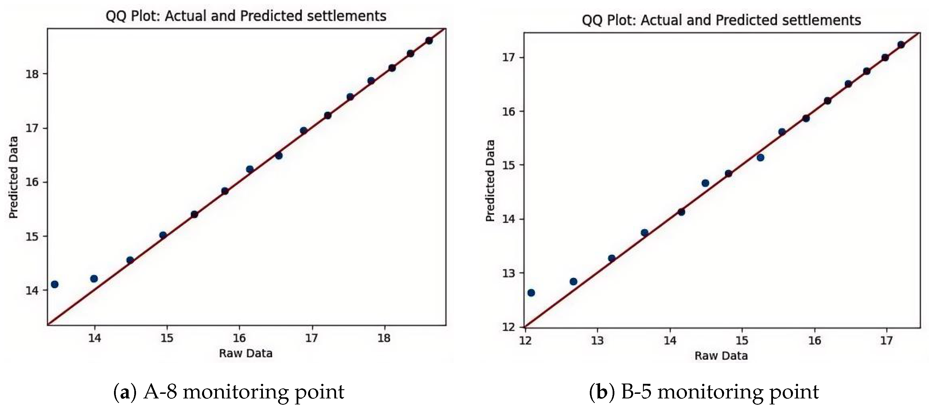
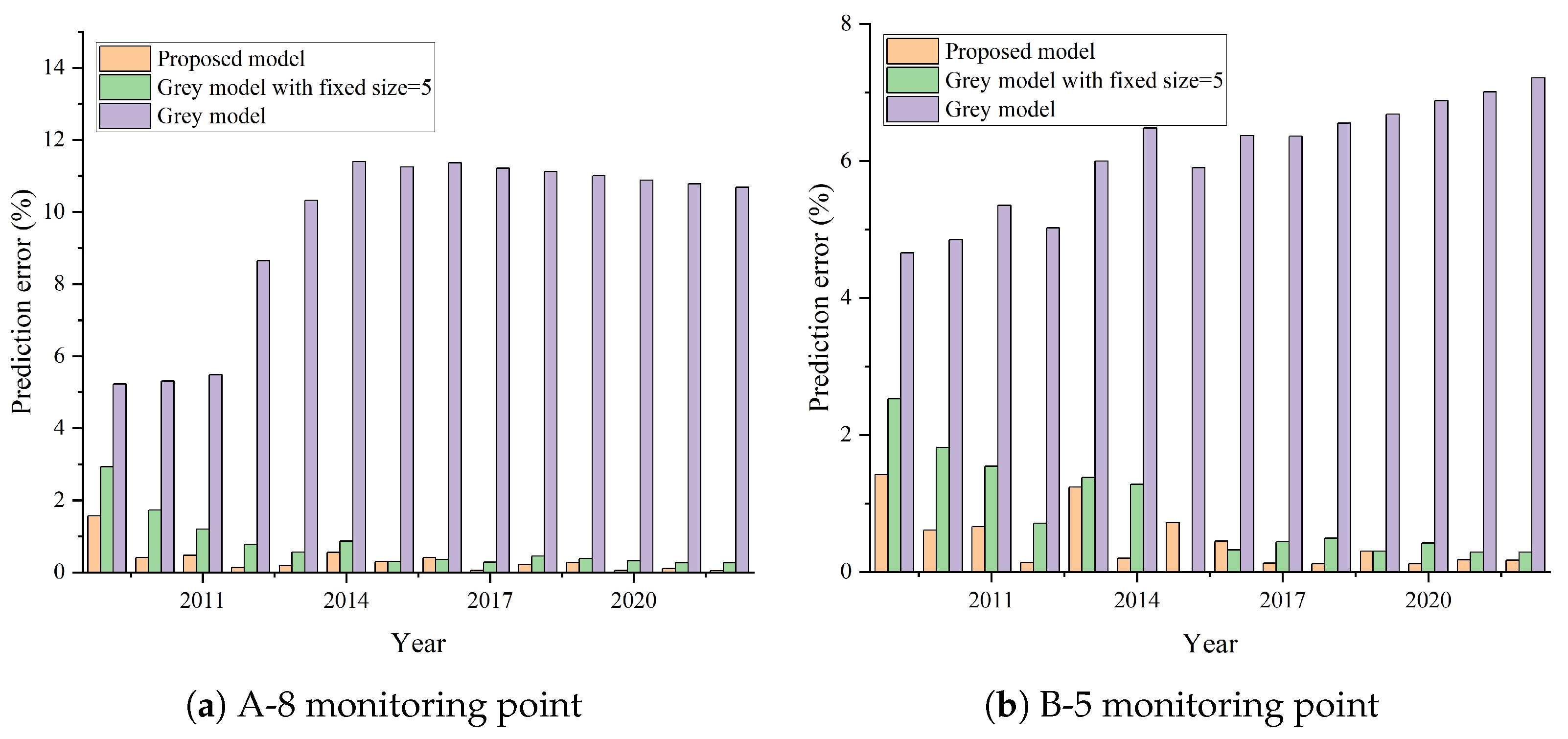
3.1. Settlement Prediction Experiment on Kansai International Airport Dataset

This section utilizes publicly available settlement data from Kansai International Airport (http://www.kansai-airports.co.jp/efforts/our-tech/kix/sink/sink3/sink3_e.html, accessed on 31 August 2024) to verify the prediction accuracy of the proposed dynamic grey model, where the settlement of each monitoring point is recorded every year. The monitoring data from the A-8 and B-5 monitoring point at Kansai International Airport from 2003 to 2022 are used as inputs for comparison experiments between the traditional grey prediction model, the grey prediction model with a fixed-size sliding window, and the dynamic grey prediction model proposed in this study. For the proposed model, the equidistant mechanism is used, and the interval of the time series is one year.

Figure 4a shows the comparative experimental results of the settlement predictions for Kansai International Airport A-8 monitoring point. The results show that the traditional grey model can effectively predict settlement for the first 4 years, but after 2012, the accuracy is low, with a prediction deviation of more than 2 m. The proposed model can continuously and effectively predict settlement, with a prediction deviation of less than 0.1 m for the last few years. Moreover, the proposed model can use existing data to predict settlement after 2 years, making it more accurate than the traditional grey model.

Figure 5a,b shows QQ plots of the actual and predicted values using the three models and for different years at Kansai International Airport. The figure illustrates the one-year prediction results obtained using the proposed model. The data points closely align with the y = x line, demonstrating strong agreement between the predicted values and the actual monitoring data.

Figure 6a and

Table 1. Experimental results of Kansai International Airport A-8 monitoring point.

	Measured Value (m)	Proposed Model			Grey Model		Fixed-Size Window
		Next 1	Next 2		Next 1		Next 1	Next 2
2003	8.55	-	-		-		-	-
2004	9.87	-	-		-		-	-
2005	11.13	-	-		-		-	-
2006	12.08	-	-		-		-	-
2007	12.82	-	-		-		-	-
2008	13.45	4.91%	-		4.91%		4.91%	-
2009	13.99	1.57%	9.79%		5.22%		2.93%	9.79%
2010	14.49	0.41%	3.52%		5.31%		1.73%	5.73%
2011	14.94	0.47%	1.27%		5.49%		1.20%	3.61%
2012	15.38	0.13%	1.04%		8.65%		0.78%	2.41%
2013	15.80	0.19%	0.51%		10.32%		0.57%	1.58%
2014	16.14	0.56%	0.99%		11.40%		0.87%	1.61%
2015	16.54	−0.30%	0.79%		11.25%		0.30%	1.27%
2016	16.88	0.41%	1.90%		11.37%		0.36%	0.89%
2017	17.22	0.06%	0.87%		11.21%		0.29%	0.75%
2018	17.53	0.23%	0.29%		11.12%		0.46%	0.74%
2019	17.82	0.28%	0.62%		11.00%		0.39%	0.95%
2020	18.10	0.06%	0.61%		10.88%		0.33%	0.77%
2021	18.36	0.11%	0.27%		10.78%		0.27%	0.71%
2022	18.61	0.05%	0.32%		10.69%		0.27%	0.59%
RSME	-	0.1851	0.4145		1.6395		0.2615	0.4857
t-value (DF = 13)	-	−2.8494	−2.6659		−12.3249		−3.8979	−3.5789

present the settlement data for the A-8 monitoring point at Kansai International Airport from 2003 to 2022, along with the deviation results obtained using the three prediction models. For the traditional grey model, only the next position of the existing data sequence is predicted (e.g., using the settlement data sequence from 2003 to 2012 to predict settlement in 2013, or comparing the predicted result with the monitored value in 2013 to obtain the prediction error). In the other two prediction models, the next one to three positions of the existing data sequence can be predicted effectively.

Table 1 shows that the soil settlement prediction accuracy using the traditional grey model is poor, with errors exceeding 10%. Based on the traditional grey model, adding a fixed-size sliding window mechanism (with a size of 5) can effectively predict the next one to three positions of the existing data sequence. Using the proposed model, the prediction accuracy can be further improved based on the fixed-size sliding window grey model. According to the experimental results, the proposed model maintains prediction deviation below 0.5% when forecasting the next position in the data sequence. For the next two to three positions, the prediction deviation remains below 2% in most cases, except for certain instances (e.g., predicting settlement in 2014 using data from 2003 to 2011). Among the three models, the proposed model consistently demonstrates the highest prediction accuracy. Additionally, the t-test results for the last 14 years (with a degree of freedom of 13) indicate that the proposed model outperforms both the traditional grey model and the grey model with a fixed-size sliding window. The absolute value of t for the proposed model is less than 3, significantly lower than those of the other two models, confirming its superior performance.

Figure 4b shows the comparative experimental results of settlement predictions for the Kansai International Airport B-5 monitoring points. The settlement variation shows that the prediction deviation of the traditional grey model increases with time, with deviation of more than 1.2 m in 2022. The proposed model can continuously and effectively predict settlement, with a prediction deviation of less than 0.1 m for the last few years. Moreover, the proposed model can use existing data to predict settlement after 2 years, making it more accurate than the traditional grey model.

Figure 6b and

Table 2. Experimental results of Kansai International Airport B-5 monitoring point.

	Measured Value (m)	Proposed Model			Grey Model		Fixed-Size Window
		Next 1	Next 2		Next 1		Next 1	Next 2
2003	7.20	-	-		-		-	-
2004	8.75	-	-		-		-	-
2005	9.89	-	-		-		-	-
2006	10.72	-	-		-		-	-
2007	11.46	-	-		-		-	-
2008	12.08	4.55%	-		4.55%		4.55%	-
2009	12.66	1.42%	8.85%		4.66%		2.53%	8.85%
2010	13.19	0.61%	3.34%		4.85%		1.82%	5.16%
2011	13.65	0.66%	1.83%		5.35%		1.54%	3.88%
2012	14.15	−0.14%	1.13%		5.02%		0.71%	2.61%
2013	14.49	1.24%	0.90%		6.00%		1.38%	2.48%
2014	14.81	0.20%	2.70%		6.48%		1.28%	2.90%
2015	15.25	−0.72%	−0.39%		5.90%		0.00%	1.44%
2016	15.55	0.45%	−0.51%		6.37%		0.32%	0.77%
2017	15.88	−0.13%	0.94%		6.36%		0.44%	0.69%
2018	16.18	0.12%	−0.06%		6.55%		0.49%	0.99%
2019	16.46	0.30%	0.43%		6.68%		0.30%	1.09%
2020	16.72	0.12%	0.72%		6.88%		0.42%	0.72%
2021	16.97	0.18%	0.35%		7.01%		0.29%	0.82%
2022	17.20	0.17%	0.47%		7.21%		0.29%	0.70%
RSME	-	0.1644	0.3561		0.9379		0.2031	0.4335
t-value (DF = 13)	-	−2.2205	−2.4865		−16.9147		−4.778	−4.3224

present the settlement data for monitoring point B-5 at Kansai International Airport from 2003 to 2022, and the deviation results of the predictions made using the three different models are presented. Table 2 shows that the traditional grey model exhibits high prediction deviations for soil settlement. After adding the fixed-size sliding window mechanism, predictions for the next one to three positions in the existing data sequence can be effectively made. The experimental results demonstrate that the proposed model achieves a prediction error of less than 1% when predicting the next position in the data sequence. For predictions of the next two to three positions, the error remains below 3% in most cases, with only a few exceptions. Among the three models, the proposed model consistently delivers the highest prediction accuracy. Furthermore, the t-test results for the last 14 years (with a degree of freedom of 13) confirm that the proposed model outperforms both the traditional grey model and the grey model with a fixed-size sliding window. The absolute value of t for the proposed model is less than 2.5, significantly lower than those of the other two models, underscoring its superior performance.

3.2. Settlement Prediction Experiment on Data from Xiamen Xiang’an International Airport

This section uses the settlement data of Xiamen Xiang’an International Airport obtained in ref. [30], which include the deformation data of six monitoring points at Xiamen Xiang’an International Airport. The monitoring data from 2016 to 2020 are used as inputs for comparison experiments between the dynamic grey prediction model proposed in this study, the grey prediction model with a fixed-size sliding window, and the traditional grey prediction model. For the proposed model, the equidistant mechanism is used, and the interval of the time series is 0.25 years.

Figure 7a–e shows the comparative experimental results of settlement predictions for the different monitoring points. The experimental results demonstrate that the proposed prediction model more effectively captures the variations in airport settlement and delivers more accurate predictions. Except for a few specific time periods (e.g., around June 2017 for monitoring points P1 and P2, and around January 2018 for monitoring point P3), the settlement prediction error of the proposed model remains below 2 mm. While the grey model with a fixed window performs slightly less effectively, its results are acceptable. In contrast, the traditional grey model produces significant errors, with these inaccuracies compounding over time.

Figure 8a–e show QQ plots of the actual and predicted values obtained using the three models and in different years at Xiamen Xiang’an International Airport. The figure illustrates the one-year prediction results obtained using the proposed model. The data points closely align with the y = x line, demonstrating strong agreement between the predicted values and the actual monitoring data.

Figure 9a presents the root-mean-square error (RMSE) of the proposed model, grey model with a fixed size, and the fitting methods proposed in ref. [30]. The experimental results demonstrate that the proposed prediction model consistently achieves the lowest root-mean-square error (RMSE) across all monitoring points. Furthermore, excluding a few specific time periods (e.g., around June 2017 for monitoring points P1 and P2, and around January 2018 for monitoring point P3), the RMSE of the proposed model is even lower. The RMSE of the grey model with a fixed window is also within an acceptable range, roughly aligning with the hyperbolic fitting model referenced in the literature. In contrast, the prediction errors of the traditional grey model are significantly larger and deemed unacceptable. Overall, the proposed prediction model exhibits outstanding prediction accuracy.

Figure 9b presents the t-test results, showing that, in most cases, the proposed model performs either the best or second best. Additionally, the average absolute t-value for the proposed model is less than 1.5, outperforming all three fitting methods described in ref. [30] and the other two grey models. This confirms that the proposed model delivers superior performance.

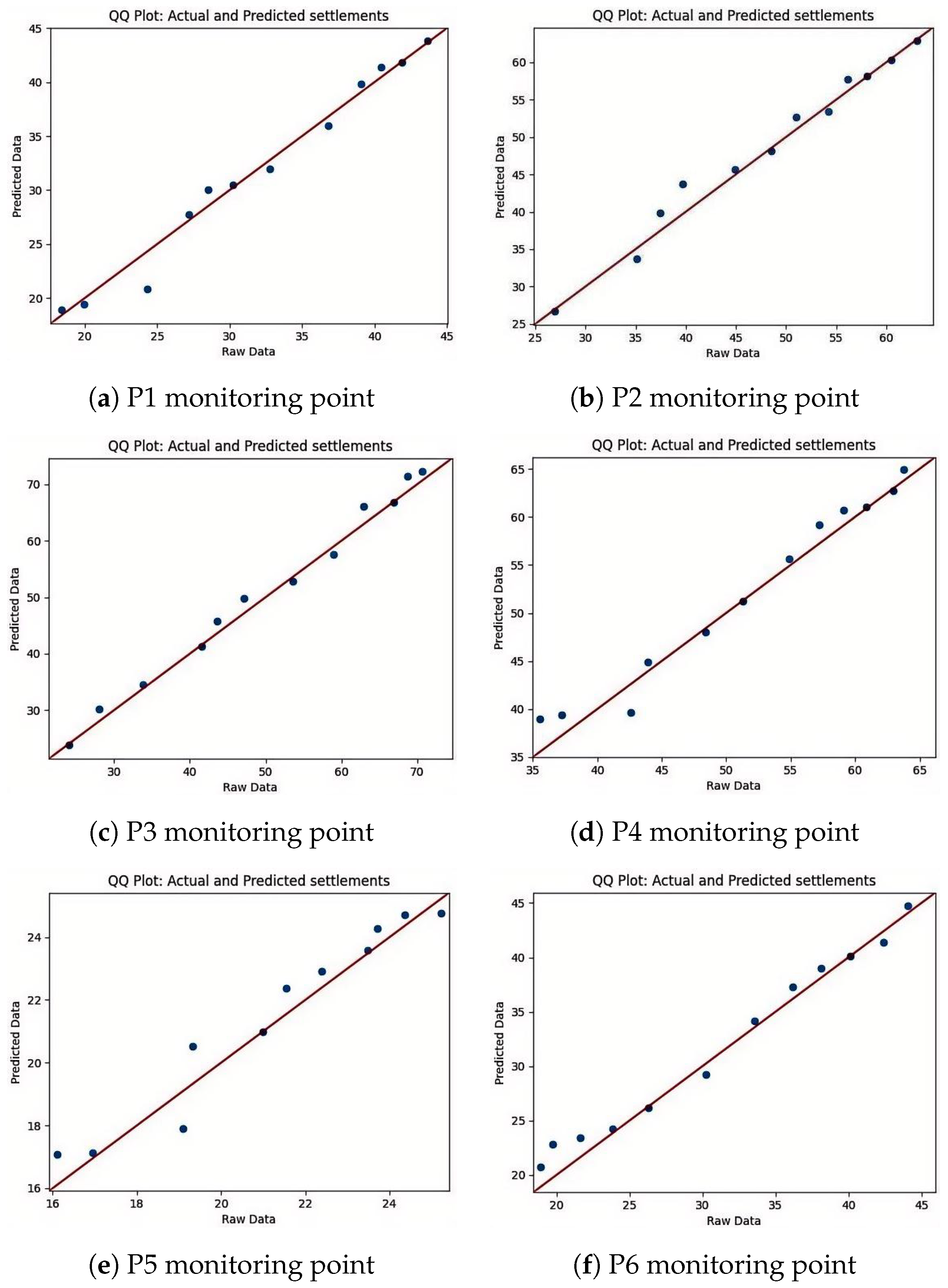
3.3. Settlement Prediction Experiment on Data from Shanghai Pudong International Airport

In this section, the monitoring data from the P215 and P230 monitoring points at Shanghai Pudong International Airport from 1998 to 2010 are used as inputs for the predictions of the dynamic grey model proposed in this study. Shanghai Pudong International Airport is not an offshore reclaimed airport, but it has a typical soft soil foundation. Therefore, settlement prediction for this airport is equally important. In the prediction of settlement at Pudong International Airport, the exponential increment mechanism is employed. During the experiment, settlement data from each year are used to predict the settlement conditions for the following 0.5 years, 1 year, and 1.5 years. For example, data from March 2000 to March 2001 are used to predict settlement from April to September 2001, April 2001 to March 2002, and April 2001 to September 2002.

Figure 10a,b shows the settlement prediction results for monitoring points P215 and P230. The experimental results show that the proposed prediction model effectively forecasts airport settlement in most cases. As shown in the figures, the prediction performance for the period from 2001 to 2003 is less accurate compared to that for other periods. This is attributed to the lack of settlement monitoring data during this time, requiring older data to be used for the simulation, which diminishes the prediction accuracy. When monitoring data are recorded consistently, the proposed model efficiently leverages a limited amount of historical data (from the last year) to predict long-term settlement conditions over the next 0.5 to 1.5 years.

4. Discussion

4.1. Performance and Comparisons Between Different Models

This study presents a dynamic grey model based on the GM(1,1) grey model and sliding window technology. The model is designed to utilize a small amount of recent settlement data to perform accurate predictions. Additionally, the sliding window size can be flexibly adjusted to improve prediction accuracy. As long as some monitoring data are available, the model maintains robustness and accuracy, making it applicable across various scenarios.

The model also incorporates two preprocessing mechanisms tailored to different prediction scenarios. The equidistant mechanism is ideal for short-term settlement predictions, such as using one year of settlement data to forecast settlement over the next three months. Conversely, the exponential increment mechanism is better suited for long-term predictions, such as leveraging one year of data to estimate settlement over a decade. While the equidistant mechanism typically delivers higher accuracy, the two mechanisms can be used simultaneously to complement each other, enhancing the model’s adaptability to diverse prediction scenarios.

Table 3. Comparisons between different models.

	Dynamic	Requirements for Data	Demand for Resources
Proposed model	Yes	Small size, easy to obtain	Low
Models based on consolidation theory	No	Small size, easy to obtain	Moderate
Models based on function fitting	No	Small size, easy to obtain	Low
Models based on machine learning	Yes/no	Big size, difficult to obtain	High
Other grey system-based models	No	Small size, easy to obtain	Low

compares the proposed model with models based on consolidation theory, function fitting, machine learning, and other grey system-based approaches. Unlike other grey system-based models, the proposed model incorporates sliding window technology, enabling it to utilize the most recent monitoring data for prediction. This makes it a dynamic prediction model.

While some machine-learning algorithms are also dynamic, their prediction models often require large amounts of high-dimensional data for effective modeling. However, in practical single engineering projects, obtaining sufficient valid data can be challenging, which negatively impacts prediction accuracy. The other models lack a mechanism for dynamic prediction.

Compared to these alternatives, the proposed prediction model demonstrates superior performance.

4.2. Future Directions

Further research could focus on the following areas:

(1) Expansion to different grey models and data preprocessing methods: The dynamic grey model proposed in this study is based on the traditional GM(1,1) grey model and employs a simple mean-difference method for data preprocessing. Depending on the application requirements, other grey models, such as GM(1,n) or GM(2,1), could also be utilized. This study considered predicting settlement based on previous settlement monitoring data. I have checked. However, if additional multidimensional data—parameters that collectively influence settlement—were available, the GM(1,n) model would likely be more effective. Furthermore, if rapid detection of settlement acceleration is required, the GM(2,1) model would be more appropriate. By combining sliding window techniques with various data preprocessing approaches, dynamic models tailored to a wider range of scenarios could be developed. In that case, the dynamic prediction framework demonstrates significantly enhanced applicability across diverse operational scenarios [31,32].

The GM(1,n) model enhances predictive interpretability in complex scenarios through multivariate expansion, though this requires increased data acquisition costs (collecting multi-dimensional parameters) and enables the incorporation of geotechnical variables (e.g., soil permeability) and environmental factors (e.g., groundwater fluctuations) as auxiliary inputs—a capability absent in the univariate GM(1,1) framework. In contrast, the GM(2,1) model strengthens nonlinear adaptability via second-order dynamic modeling, but demands extended monitoring sequences (typically more than 10 data points), achieving superior performance in long-term nonlinear settlement prediction where conventional first-order models exhibit progressive error accumulation.

(2) Enhancing early warning systems: The proposed model demonstrates strong predictive performance and can also be effectively applied to early warning systems. If significant deviations between monitoring data and predicted settlement values persist over a certain period, an early warning can be issued.

For instance, the proposed prediction model can be seamlessly integrated into airport infrastructure monitoring and maintenance systems. By continuously comparing real-time monitoring data with predicted settlement values, the model can promptly detect significant deviations, assess potential risks, and issue timely warnings. For example, if the monitored settlement exceeds the predicted value by X cm and this discrepancy continues for N consecutive days (X and N should be calculated depending on factors such as soil type, foundation conditions, and external loads), the model can trigger an early warning to highlight potential issues.

(3) Integration of physical significance into dynamic grey models: The dynamic grey prediction model proposed in this study is purely a mathematical model driven by monitoring data, without requiring an analysis of the physical mechanisms behind settlement. Future research could achieve more accurate predictions by integrating data-driven methods with the physical principles underlying settlement behavior. For instance, physical mechanisms such as soil consolidation, secondary settlement, and creep deformation can be used to constrain the prediction range of the model proposed in this study.

(4) Application to other settlement predictions: The settlement prediction model proposed in this study is a versatile dynamic forecasting model that can be used for predictions as long as continuous monitoring data are available. It is believed that this model can be applied to other settlement prediction scenarios, particularly in settlement predictions for building construction in other land reclamation projects.

5. Conclusions

Based on grey system theory and sliding window techniques, this study proposes a dynamic model for airport settlement prediction. The model evaluates predictions using the most recent data and refines its forecasting capability by dynamically adjusting the sliding window size. In addition, two mechanisms—an equidistant mechanism and an exponential mechanism—are integrated into the model to address short-term and long-term settlement prediction scenarios, respectively. For short-term predictions, comparative experiments using historical settlement data from Kansai International Airport and Xiamen Xiang’an International Airport—two offshore reclaimed airports—demonstrated an improvement in accuracy of over 20% compared to existing models. In the long-term scenario, effective predictions were obtained using historical data from Pudong International Airport, which is constructed on a soft alluvial deposit. The proposed forecasting model is purely mathematical, eliminating the need to account for numerous physical parameters, and is straightforward to implement. However, the model relies solely on a single dimension of real-time monitoring data (i.e., historical settlement data); although it provides an interpolation method to estimate data at specific time points, it still requires high-quality monitoring data and a sufficient acquisition frequency. Poor data quality or prolonged gaps in data collection may significantly compromise the model’s predictive accuracy. Incorporated multidimensional data monitoring can be used to mitigate potential issues arising from data gaps.

References

1. Mesri, G.; Funk, J. Settlement of the Kansai international airport islands. J. Geotech. Geoenviron. Eng. 2015, 141, 04014102. [Google Scholar]
2. Dan, G.; Sultan, N.; Savoye, B. The 1979 Nice harbour catastrophe revisited: Trigger mechanism inferred from geotechnical measurements and numerical modelling. Mar. Geol. 2007, 245, 40–64. [Google Scholar]
3. Fujima, K.; Shigihara, Y.; Tomita, T.; Honda, K.; Nobuoka, H.; Hanzawa, M.; Fujii, H.; Ohtani, H.; Orishimo, S.; Tatsumi, M.; et al. Survey results of the Indian Ocean tsunami in the Maldives. Coast. Eng. J. 2006, 48, 81–97. [Google Scholar]
4. Shi, X.S.; Zhao, J. Practical estimation of compression behavior of clayey/silty sands using equivalent void-ratio concept. J. Geotech. Geoenviron. Eng. 2020, 146, 04020046. [Google Scholar]
5. Nikakhtar, L.; Zare, S.; Nasirabad, H.M.; Ferdosi, B. Application of ANN-PSO algorithm based on FDM numerical modelling for back analysis of EPB TBM tunneling parameters. Eur. J. Environ. Civ. Eng. 2022, 26, 3169–3186. [Google Scholar] [CrossRef]
6. Liu, C.; Wang, Z.; Liu, H.; Cui, J.; Huang, X.; Ma, L.; Zheng, S. Prediction of surface settlement caused by synchronous grouting during shield tunneling in coarse-grained soils: A combined FEM and machine learning approach. Undergr. Space 2024, 16, 206–223. [Google Scholar] [CrossRef]
7. Feng, W.Q.; Yin, J.H. A new simplified Hypothesis B method for calculating consolidation settlements of double soil layers exhibiting creep. Int. J. Numer. Anal. Methods Geomech. 2017, 41, 899–917. [Google Scholar]
8. Nour, A.; Slimani, A.; Laouami, N. Foundation settlement statistics via finite element analysis. Comput. Geotech. 2002, 29, 641–672. [Google Scholar]
9. Sexton, B.G.; McCabe, B.A.; Castro, J. Appraising stone column settlement prediction methods using finite element analyses. Acta Geotech. 2014, 9, 993–1011. [Google Scholar]
10. Al-Shamrani, M.A. Applicability of the rectangular hyperbolic method to settlement predictions of sabkha soils. Geotech. Geol. Eng. 2004, 22, 563–587. [Google Scholar]
11. Fan, H.; Chen, Z.; Shen, J.; Cheng, J.; Chen, D.; Jiao, P. Buckling of steel tanks under measured settlement based on Poisson curve prediction model. Thin-Walled Struct. 2016, 106, 284–293. [Google Scholar] [CrossRef]
12. Zhu, L.; Xing, X.; Zhu, Y.; Peng, W.; Yuan, Z.; Xia, Q. An advanced time-series InSAR approach based on poisson curve for soft clay highway deformation monitoring. IEEE J. Sel. Top. Appl. Earth Obs. Remote Sens. 2021, 14, 7682–7698. [Google Scholar]
13. Wang, B.; Wang, X.; Ma, X. Study on optimal combination settlement prediction model based on logistic curve and Gompertz curve. Stavební Obz.-Civ. Eng. J. 2020, 29, 347–357. [Google Scholar]
14. Pulket, T.; Arditi, D. Construction litigation prediction system using ant colony optimization. Constr. Manag. Econ. 2009, 27, 241–251. [Google Scholar]
15. Song, Z.; Liu, S.; Jiang, M.; Yao, S. Research on the Settlement Prediction Model of Foundation Pit Based on the Improved PSO-SVM Model. Sci. Program. 2022, 2022, 1921378. [Google Scholar]
16. Yang, P.; Yong, W.; Li, C.; Peng, K.; Wei, W.; Qiu, Y.; Zhou, J. Hybrid random forest-based models for earth pressure balance tunneling-induced ground settlement prediction. Appl. Sci. 2023, 13, 2574. [Google Scholar] [CrossRef]
17. Xie, X.; Pan, C. Safety Prediction of Deep Foundation Pit Based on Neural Network and Entropy Fuzzy Evaluation. E3S Web Conf. 2021, 233, 03001. [Google Scholar]
18. Cao, Y.; Zhou, X.; Yan, K. Deep learning neural network model for tunnel ground surface settlement prediction based on sensor data. Math. Probl. Eng. 2021, 2021, 9488892. [Google Scholar]
19. Xie, S.L.; Hu, A.; Wang, M.; Xiao, Z.R.; Li, T.; Wang, C. 1DCNN-based prediction methods for subsequent settlement of subgrade with limited monitoring data. Eur. J. Environ. Civ. Eng. 2025, 29, 759–784. [Google Scholar]
20. Deng, J.L. Control problems of grey systems. Syst. Control Lett. 1982, 1, 288–294. [Google Scholar]
21. Tong, M.; Yan, Z.; Chao, L. Research on a grey prediction model of population growth based on a logistic approach. Discret. Dyn. Nat. Soc. 2020, 2020, 2416840. [Google Scholar] [CrossRef]
22. Li, B.; He, C.; Hu, L.; Li, Y. Dynamical analysis on influencing factors of grain production in Henan province based on grey systems theory. Grey Syst. Theory Appl. 2012, 2, 45–53. [Google Scholar]
23. Liu, C.; Xie, W.; Lao, T.; Yao, Y.t.; Zhang, J. Application of a novel grey forecasting model with time power term to predict China’s GDP. Grey Syst. Theory Appl. 2021, 11, 343–357. [Google Scholar] [CrossRef]
24. Zhang, W.; Xiao, R.; Shi, B.; Zhu, H.h.; Sun, Y.j. Forecasting slope deformation field using correlated grey model updated with time correction factor and background value optimization. Eng. Geol. 2019, 260, 105215. [Google Scholar] [CrossRef]
25. Wu, L.; Li, S.; Huang, R.; Xu, Q. A new grey prediction model and its application to predicting landslide displacement. Appl. Soft Comput. 2020, 95, 106543. [Google Scholar]
26. Jin, S.J.; Zhang, D.S.; Shu, Z.; Zhao, Y. Grey model theory used in prediction of subgrade settlement. Appl. Mech. Mater. 2012, 105, 1576–1579. [Google Scholar] [CrossRef]
27. Wang, Y.; Yang, G. Prediction of composite foundation settlement based on multi-variable gray model. Appl. Mech. Mater. 2014, 580, 669–673. [Google Scholar] [CrossRef]
28. Zhang, J.; Qin, Y.; Zhang, X.; Che, G.; Sun, X.; Duo, H. Application of non-equidistant GM(1,1) model based on the fractional-order accumulation in building settlement monitoring. J. Intell. Fuzzy Syst. 2022, 42, 1559–1573. [Google Scholar] [CrossRef]
29. Zhang, C.; Li, J.z.; He, Y. Application of optimized grey discrete Verhulst–BP neural network model in settlement prediction of foundation pit. Environ. Earth Sci. 2019, 78, 441. [Google Scholar] [CrossRef]
30. Xiong, Z.; Deng, K.; Feng, G.; Miao, L.; Li, K.; He, C.; He, Y. Settlement prediction of reclaimed coastal airports with InSAR observation: A case study of the Xiamen Xiang’an International Airport, China. Remote Sens. 2022, 14, 3081. [Google Scholar] [CrossRef]
31. Zeng, J.J.; Feng, P.; Dai, J.G.; Zhuge, Y. Development and behavior of novel FRP-UHPC tubular members. Eng. Struct. 2022, 266, 114540. [Google Scholar]
32. Douglas, I.; Lawson, N. Airport construction: Materials use and geomorphic change. J. Air Transp. Manag. 2003, 9, 177–185. [Google Scholar]
Figure 1. Flow chart of dynamic grey model.
Buildings 15 01034 g001
Figure 2. An example of a sliding window (size: 5).
Buildings 15 01034 g002
Figure 3. Flow chart of prediction (using exponential increment mechanism).
Buildings 15 01034 g003
Figure 4. Experimental results of settlement predictions at Kansai International Airport.
Buildings 15 01034 g004
Figure 5. Experimental results of QQ plots at Kansai International Airport.
Buildings 15 01034 g005
Figure 6. Experimental results of prediction errors at Kansai International Airport.
Buildings 15 01034 g006
Figure 7. Experimental results of settlement predictions at Xiamen Xiang’an Airport.
Buildings 15 01034 g007
Figure 8. Experimental results of QQ plots at Xiamen Xiang’an Airport.
Buildings 15 01034 g008
Figure 9. Experimental results of settlement predictions at Xiamen Xiang’an International Airport.
Buildings 15 01034 g009
Figure 10. Experimental results of settlement predictions at Shanghai Pudong International Airport.
Buildings 15 01034 g010