Integrated Optimization System for Geotechnical Parameter Inversion Using ABAQUS, Python, and MATLAB

Abstract

Accurate inversion of geotechnical parameters is essential for assessing foundation-bearing capacity and stability, which directly impact structural safety and serviceability. Accurate prediction of load settlement behavior is crucial to prevent overdesign and underperformance, ensuring that foundations support anticipated loads without excessive deformation or failure. This paper presents an integrated optimization system combining ABAQUS (2022), Python (PyCharm21.3.3), and MATLAB (2022b) software, based on the Duncan–Chang (DC) model, for inversion of key geotechnical parameters. The ABAQUS UMAT subroutine customizes the DC model, facilitating its application in finite element simulations for soil–structure interaction analysis. To improve the optimization process, an adaptive genetic algorithm that dynamically adjusts crossover and mutation rates, thereby improving solution searches and parameter space exploration, is implemented. Key parameters of the DC model—the initial tangent stiffness (K) and nonlinear deformation characteristics (n) of soil—are inverted. The accuracy of this inversion is validated through comparisons with experimental pressure–settlement curves obtained from indoor bearing plate tests. Therefore, this optimization system effectively integrates intelligent algorithms with finite element analysis, serving as a reliable tool for precise geotechnical parameter inversion, with potential for improving foundation design accuracy, optimizing soil–structure interaction predictions, and improving the overall stability and safety of geotechnical structures.

1. Introduction

Predicting pressure–settlement (p–s) curves of foundations is crucial in geotechnical engineering, enabling accurate estimation of post-construction settlements. Reliable p–s curve predictions help prevent structural damage, preserve serviceability, and mitigate the risk of catastrophic failures [1]. Understanding settlement behavior is crucial for designing foundations capable of accommodating the expected deformations without compromising structural performance [2].

Several studies have focused on predicting p–s settlement curves during the elastic deformation stage of foundations before overall shear failure. Current methodologies, including the layered summation method recommended by the Chinese Code for the Design of Foundations (GB 50007-2011) [3], involve dividing the soil mass into discrete layers and summing settlement contributions from each layer under applied loads. However, a significant limitation of the layered summation method is its assumption that soil parameters remain constant during elastic deformation. In reality, the initial tangent modulus varies with stress levels [4,5,6,7], leading to inaccuracies in settlement predictions, particularly under complex loading conditions.

Furthermore, traditional p–s curve prediction approaches often employ simplified soil models that fail to capture the inherent nonlinearities of soil behavior. Soil–structure interactions are inherently complex, and the nonlinear soil deformation characteristics under varying stress conditions are inadequately represented by these models. Moreover, conventional methods rely heavily on extensive field testing to obtain accurate soil parameters, making the process time-consuming and labor-intensive. Conducting comprehensive tests across all sections of a large-scale project site is impractical and cost-prohibitive. Consequently, there is an urgent need for more efficient and reliable methods to predict p–s curves with minimal reliance on extensive field testing.

To address these challenges, in this study, we conducted comprehensive indoor bearing plate experiments to obtain accurate p–s curve data, providing a reliable empirical foundation for parameter inversion. These experiments offer advantages such as controlled testing conditions, reduced time and labor requirements compared to those in extensive field tests, and the ability to replicate varying stress conditions to capture the nonlinear behavior of soils. Building upon the experimental data, this study introduces a joint inversion optimization system that integrates ABAQUS, Python, and MATLAB, using the Duncan–Chang (DC) model to represent soil behavior. The DC model is a widely recognized nonlinear elastic model that effectively captures the stress–strain relationships of soils and accommodates the nonlinear deformation characteristics observed in real-world scenarios [8,9,10,11,12]. A user material (UMAT) subroutine is developed in ABAQUS for the DC model [13], leveraging the superior capabilities of the finite element method in modeling complex soil–structure interactions compared to conventional plane strain or plane stress approaches [14,15,16,17]. This integration enables precise simulation of soil behavior under varying stress conditions, enhancing the reliability of settlement predictions [18,19,20]. Furthermore, this method focuses on parameter inversion based on p–s curves measured within small stress ranges, enabling the prediction of p–s curves over broader stress ranges [21]. Consequently, settlement curve testing can be performed at multiple locations across a site, providing a more comprehensive understanding of the site’s geotechnical characteristics [22,23].

The proposed inversion method leverages the robust nonlinear solving capabilities of finite element analysis combined with the precision of parameter inversion from empirical data, effectively overcoming the limitations of traditional optimization techniques prone to local optima entrapment. This integrated approach improves the accuracy of soil parameter identification and reduces the dependency on extensive field testing, streamlining the foundation design process. Validation through indoor bearing plate experiments demonstrates the efficacy of the method in accurately inverting soil parameters and predicting settlement behavior, highlighting its potential for practical engineering applications.

This study introduces a novel joint optimization system that advances geotechnical parameter inversion by combining finite element analysis with a customized inversion approach. The system’s ability to accurately invert soil parameters and predict settlement behavior under varying stress conditions offers significant improvements in foundation design reliability and efficiency, establishing a solid foundation for engineering design.

2. Physical Model Tests

A series of carefully designed controlled indoor loading tests were conducted in accordance with the established standards to ensure the reliability of the resulting data. The experimental setup included a loading plate, rigid model box, and self-balancing loading frame, arranged to simulate real-world engineering conditions. The loading plate used in the tests had dimensions of 0.5 m × 0.5 m, while the model box measured 1.4 m × 1.3 m × 1.2 m. The model box was designed to accommodate both the loading plate and the soil sample while minimizing the boundary effects that could influence soil behavior. To further minimize boundary effects, the interior walls of the model box were coated with petroleum jelly. This coating reduced the friction between the soil and walls, allowing the soil to deform more freely under load and preventing stress concentrations and deformation restrictions caused by wall–soil interactions.

The soil samples used in the experiment consisted of fully weathered mudstone cohesive soil with a sieve aperture size of 0.25 mm, ensuring uniformity and representativeness of the soil properties. The preparation process began by crushing dry soil into individual particles using tools such as shovels. Water was then added to the soil to achieve a moderately moist state, facilitating efficient compaction and handling. The moist soil was then divided into three layers, each being approximately 10 cm thick. A vibrating compactor was used to compact the middle and lower layers, with six passes applied to the middle layer and four to the lower layer to ensure sufficient soil density. Before adding the topsoil layer, the surface of the middle layer was roughened to enhance interlayer adhesion and prevent slippage. The uppermost layer was then compacted with a 9.2 kg aluminum cylinder, completing six passes to ensure uniformity. Finally, the surface was sprayed with water and left undisturbed for 48 h. This curing period allowed the soil to reach saturation, eliminating the effects of natural settlement and stabilizing the test specimen. Forty-eight-hour standing ensured that the capillary water inside the soil was fully transported and that the local moisture content difference caused by compaction during the preparation process was eliminated. During the experiments, the ambient laboratory temperature was strictly maintained at 20 °C ± 2 °C, and natural airflow conditions were maintained without forced airflow to avoid excessive evaporation from the specimen surfaces. The initial moisture content of the soil specimens was controlled at 18% ± 0.5% (determined using the oven-drying method). In addition, the specimens were covered with plastic film during the 48 h curing period to minimize water loss and ensure that the variations in moisture content were negligible.

The test was conducted in strict accordance with GB 50007-2011, which explicitly specifies that, for shallow plate loading tests on soils, the area of the loading plate must be no smaller than 0.25 m². In addition, the specifications align closely with the international standard ISO 22477-2:2015 [24], which outlines the requirements for shallow plate loading tests, recommending loading plate diameters ranging from 300 to 750 mm and a thickness no less than 25 mm, determined according to specific test requirements and soil conditions. Both standards were consistent regarding the dimensional criteria for the loading plates used in the shallow foundation tests. A 0.5 m × 0.5 m load plate was placed on the prepared soil surface, supported by a multilayer canvas and airbags. This setup ensured a uniform load distribution and prevented direct contact between the load plate and soil, thereby reducing the risk of premature edge failure. As Figure 1 illustrates, the system’s key components included a square flexible bearing plate and an inductive displacement sensor. The inductive displacement sensor measured the movement of the airbag within the square flexible bearing plate, providing precise data on soil deformation under load.

Figure 1a shows a square flexible pressure plate consisting of a steel box, steel frame, airbag, and multilayer canvas. The steel box, constructed from horizontal and vertical steel plates, primarily bears pressure, protects it, and constrains the airbag. It was made of 304 stainless steel with a yield strength of 210 MPa. The overall height of the steel box was 48 mm (including an 8 mm thick horizontal steel plate). The side length was 510 mm (with a 5 mm thick vertical steel plate), and two holes were drilled in the horizontal steel plate for the pump (exhaust) port and wire passage. The steel frame, comprising eight Q235 steel pipes and Q235 iron plates, has thick iron plates and a steel pipe outer diameter of 40 mm. Its main function is to enhance the bending strength of the pressure plate structure, thereby increasing the load-bearing capacity of the device. The airbag, installed beneath the steel box, maintains a uniform internal air pressure to ensure even soil loading, while the multilayer canvas protects the airbag. The design of the steel box and steel frame ensures that the bearing threshold of the structure reaches 500 kPa. For convenience, the steel frame was not placed between the jack and bearing plate during this test.

Figure 1b shows that inductive displacement sensors typically employ self-inductance or mutual inductance methods when measuring displacement. These sensors mainly consist of a solenoid coil and an iron core connected to the measured object. As the measured object moves, the iron core within the coil alters the coil’s inductance, reflecting the displacement through changes in inductance.

The loading apparatus consiste of a self-balancing loading frame comprising upper and lower frames. The lower frame measuring 1.4 m × 1.3 m × 1.2 m was constructed from 12 square steel tubes, each with 60 mm sides and 5 mm thicknesses, welded together. The base of the lower frame was reinforced with channel steel, whereas the perimeter was fitted with thin-walled C-shaped galvanized steel sheets as retaining walls. The upper reaction frame was made of square steel tubes with 40 mm sides and a 4 mm thickness, welded together. A central platform 350 mm wide was securely fastened to four vertical posts, allowing the hydraulic jack to exert an upward force. To prevent direct contact between the loading plate and soil, a controlled amount of air was pumped into the airbags beneath the loading plate, slightly inflating them. This inflation gently elevated the loading plate, thereby preventing premature damage to the soil edges. The loading plate was then positioned atop multiple layers of canvas, which were wrapped around the steel casing to ensure a uniform load distribution. The hydraulic jack, pressure sensor, and reaction frame were securely positioned on the loading plate and fastened with bolts. An inductive displacement sensor was connected to the loading plate, and a micrometer was mounted on a magnetic base. The micrometer probe was carefully aligned with the displacement sensor to ensure precise displacement measurements. A uniformly distributed load ranging from 0 kPa to 160 kPa was applied to the flexible bearing plate using a hydraulic jack mounted in a self-balancing frame. After each incremental load application, sufficient time was allowed to elapse to ensure that initial soil consolidation was achieved. During the loading process, the two operators oversaw the experiment. The operator on the left controlled the air pump according to the pressure gauge reading and recorded the data from the inductive displacement sensor (δ) and micrometer (δ’). The readings from the displacement sensor and micrometer represented the displacement in the air cushion and plate settlement, respectively. The operator on the right managed the oil pump rod according to the force display (P) reading. Because fully weathered argillaceous soil deforms rapidly under load, precise and coordinated data collection was essential. The total settlement (S) was determined as the sum of the displacements measured by the inductive sensor (δ) and the micrometer (δ′), i.e., S = δ + δ′. This integrated measurement approach provided a comprehensive evaluation of the deformation of the soil under loading. During the loading process, the reaction frame experienced upward forces from the hydraulic jack which were transmitted to the lower frame through four bolts. The self-weight of the soil sample, combined with the applied load on the loading plate, counterbalanced these upward forces and maintained equilibrium during testing. Figure 2 illustrates the calibration procedure employed for the displacement sensors. Calibration was conducted by applying an external force to pull the internal iron core outward, thereby obtaining the actual displacement (δ) of the sensor. Simultaneously, the corresponding electrical readings (L) within the sensor were recorded to establish a correlation curve. The accuracy of the calibration significantly improved with increased precision of the externally applied displacement. Therefore, a custom calibration device was fabricated (see Figure 2). Specifically, a vertical ruler was mounted on a stainless steel base using a lower bracket. An extension rod connected to the sensor’s iron core (i.e., the measurement end) was extended and adhered to a PVC plate constructed by bonding two 3 mm thick PVC strips, forming a rectangular plate measuring 60 mm × 6 mm. This extension rod enabled the precise control of the displacement without interfering with sensor operation. For the calibration process, an external force incrementally moved the sensor core outward in 0.1 mm increments. The sensor measured the displacement (δ), and simultaneously, the corresponding electrical signal (L) from the LCR bridge was recorded, enabling the construction of a displacement–inductance relationship. The collected inductance values and corresponding displacements were subsequently plotted as a calibrated scatter plot, and a linear fit of the two was accomplished, accurately reflecting the sensor’s characteristics.

After completing the triaxial test on the test soil, the shear strength parameters of the soil were determined to be c = 18 kPa and φ = 28°. In this test, a displacement sensor was placed at the edge of the airbag in the load-bearing plate, and the settlement at the edge of the load-bearing plate was used for inversion. The test incorporated a flexible water pressure plate that was meticulously designed and positioned at the edge of the load-bearing plate to emulate the surcharge present at the edge of the infrastructure under operational conditions. The configuration of the flexible water pressure plate entailed the integration of a plexiglass tube, lead shot, weight box, and rectangular water bladder. The weight box consisted of a plastic container with a diminutive aperture at the center of the base into which a hollow screw was fixed. A thin rectangular water bladder was fabricated by bonding a latex film to the bottom, and an acrylic tube was inserted into the hollow screw and connected to the water bladder. During the load test, the airbag was filled with water. Subsequently, an appropriate amount of water was poured into the weight box, allowing the water in the airbag to enter the acrylic tube. The water column reached a height of 15 cm, and the surface load was measured at 1.5 kPa. Figure 3 illustrates the specific process of the loading test. It should be additionally noted that a polytetrafluoroethylene film with a thickness of 0.3 mm (Figure 3) and a friction coefficient of $\mu \approx 0.04$ was employed to significantly reduce the canveline–soil interface friction, thereby approximating smooth contact conditions. For surface flatness control, a level was used to calibrate the surface, ensuring that the horizontal error in all directions remained below 0.1° (equivalent to a water offset of <1 mm).

Figure 4 shows the settlement data from the loading test. The reason for setting the upper pressure limit to 160 kPa is as follows: During the loading process, the settlement rate increased significantly in the 128–132 kPa range, and we believe that the soil entered a local plastic state. In addition, when we loaded 150 kPa in the test, we heard abnormal sounds from the self-balancing frame likely because of the excessive number of experiments performed for a long period, and the performance was reduced. Considering the safety of field testers, we stopped the continuous loading at approximately 160 kPa.

As shown in Figure 4, in the settlement p–s curve, the settlement behavior of the soil exhibited distinct nonlinear characteristics. The initial settlement rate was relatively rapid; however, as the pressure increased, the settlement rate gradually decreased and stabilized. Notably, at higher pressures, the rate of increase in the settlement significantly decreased. This nonlinear relationship indicates that the soil is highly compressible at low pressures, whereas at high pressures, it tends to compact, resulting in slower settlement changes. This phenomenon cannot be precisely quantified using a linear model owing to the deformation characteristics of the soil under varying stress levels. This limitation is particularly evident in compressible soils, where the stress–strain relationship becomes more complex under higher loads. To ensure accurate analysis, the use of a nonlinear constitutive model such as the DC model is essential. The DC model represents the nonlinear deformation behavior of the soil through reasonable parameters.

3. DC Model and Parameters to Be Inverted

The DC model (Appendix A) [25] describes the hyperbolic stress–strain relationship of soil, and its typical tangent modulus equation is expressed as follows:

$$E_t=K\mathrm{P}\mathrm{a}{\left({\displaystyle \frac{{\sigma }_3}{\mathrm{P}\mathrm{a}}}\right)}^n{\left[1-R_f{\displaystyle \frac{{\sigma }_1-{\sigma }_3}{{\left({\sigma }_1-{\sigma }_3\right)}_f}}\right]}^2.$$

(1)

In the DC model, the parameters $K$ (modulus coefficient) and $n$ (dimensionless exponent) are selected as reflection variables. These two parameters define the variation in the tangent modulus as a function of confining pressure. Adjusting $K$ and $n$ enables an accurate representation of various stiffness magnitudes under different confining pressures. Compared to other soil constitutive models, the parameters $K$ and $n$ within the DC model are relatively more physically intuitive and sensitive to variations in confining pressure conditions. The failure ratio parameter $R_f$ is comparatively well defined, representing the ratio between the peak stress state and the ultimate stress state at failure, and typically falls between 0.6 and 0.95. It is related to the soil physical properties and failure morphology in a straightforward manner. In finite element calculations, the parameter $R_f$ mainly influences the calculated deformation behavior; when $R_f$ increases, the effects of lateral deformation become relatively prominent, while axial deformation diminishes. Conversely, smaller $R_f$ values reflect relatively rigid soil characteristics. It is typically suggested that, except in special circumstances, $R_f$ should not approach zero because actual soil behavior seldom exhibits absolute brittleness. Generally, soils experience progressive yield phenomena; hence, $R_f$ typically varies within a medium–high range, characteristically around 0.7. To determine the parameters $K$, $n$, and $R_f$ from the experimental results, regression analysis can be performed utilizing conventional triaxial compression test data.

4. Implementation of the DC Model in ABAQUS

To establish the relationship curve between the deviatoric stress and axial strain, the DC model was implemented in ABAQUS. This relationship was derived by simulating a triaxial test within a finite element framework. The next step included calculating the constitutive equation of the model to verify whether it satisfied the established requirements. The model parameters were set to a cube unit with a confining pressure of 50 kPa. The constraints of the triaxial test were incorporated, with cohesion set to 30 kPa, an internal friction angle of 20°, and a failure ratio $R_f$ of 0.9. During loading, a strain of 0.05 was gradually applied to the model’s top surface in the opposite direction to the axis. Figure 5 shows the finite element model (FEM) used in the triaxial test.

As shown in Figure 6, the axial strain and deviatoric stress were measured at one point in the model.

The principal equation of the DC model is as follows [26]:

$${\sigma }_1-{\sigma }_3={\displaystyle \frac{{\epsilon }_1}{a+b{\epsilon }_1}},$$

(2)

where ${\sigma }_1-{\sigma }_3$ is the deviatoric stress, and ${\epsilon }_1$ is the axial strain. The deviatoric strain data in Figure 2 were fitted according to Equation (2), resulting in the following equation:

$${\sigma }_1-{\sigma }_3={\displaystyle \frac{{\epsilon }_1}{0.000254+0.006{\epsilon }_1}}.$$

(3)

An initial tangent modulus $E_i$ = 4000 kPa was calculated from the inductive displacement sensor calibration curve in Figure 2. It is known that a = 1/$E_i$= 0.00025, which is close to the fitted value of 0.000254. The following mathematical relationship was used [27]:

$$b={{\displaystyle \frac{R_f}{{(\sigma }_1-{\sigma }_3)}}}_f,$$

(4)

$${\left({\sigma }_1-{\sigma }_3\right)}_f={\displaystyle \frac{2·c·\mathrm{c}\mathrm{o}\mathrm{s}\phi +2{\sigma }_3\mathrm{s}\mathrm{i}\mathrm{n}\phi }{1-\mathrm{s}\mathrm{i}\mathrm{n}\phi }}.$$

(5)

Calculations performed using Equations (4) and (5) yielded a b value of 0.006017. This demonstrates a high degree of compatibility with the constitutive equation of the DC model [28,29], thereby substantiating the efficacy of this secondary development and paving the way for subsequent steps.

5. Adaptive Genetic Algorithm

A genetic algorithm (GA) is an optimization method based on natural selection and genetic mechanisms that is employed to determine the global optimal solution for complex problems. An adaptive GA (AGA) is an enhanced version of a GA, improving its performance by adaptively adjusting parameters such as the crossover and mutation rate [30]. The AGA optimization process is given in Appendix B.

6. Joint Optimization Method

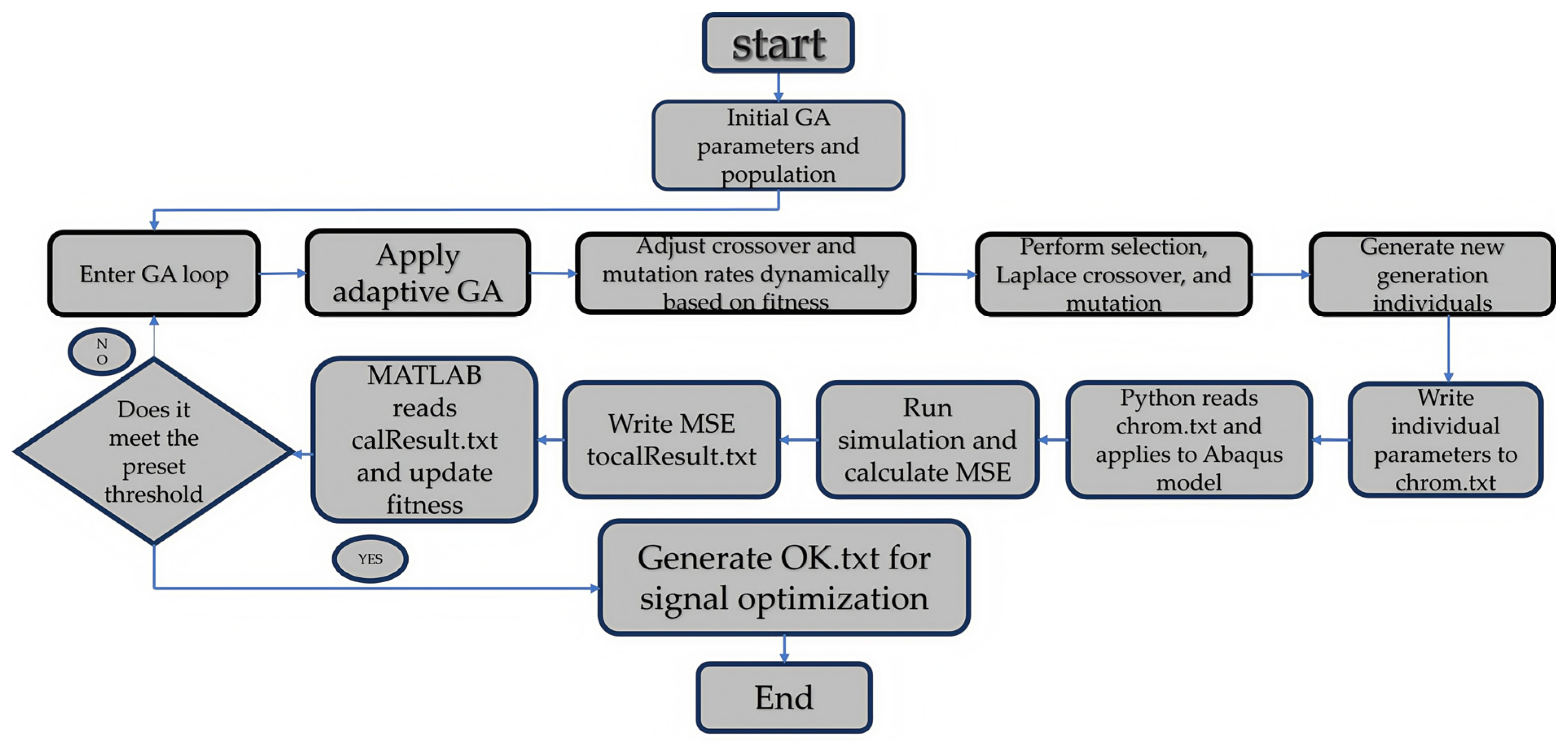
6.1. Joint Optimization Process

The joint optimization process begins with the initialization of the parameters and population for the GA, after which the system enters the main optimization loop. Using an AGA, the crossover and mutation rates are dynamically adjusted based on the fitness of the current individuals. The algorithm then performs selection, Laplacian crossover, and mutation to generate a new population. Subsequently, the system writes the parameters of these new individuals to a chrom.txt file and applies them to the ABAQUS model using Python scripts for the simulation. After the simulations are completed, the MSE for each individual is calculated, and the results are written in the calResult.txt file. MATLAB then reads the MSE values from this file, updates the fitness of each individual, and checks whether the preset optimization threshold has been reached. If the threshold is not met, the loop continues, generating new individuals and repeating the optimization steps. Once the threshold is achieved, the system generates an OK.txt file, which marks the completion of the optimization process.

Figure 7 shows a flowchart of the joint optimization method.

6.2. Application for Proposed Procedures

Prior to conducting a numerical inversion based on the experimental curves, a series of stability tests were conducted employing the following methodology. The initial parameters were set at K = 350, n = 0.35, $R_f$ = 0.8, u = 0.25, c = 18 kPa, and φ = 28°. These parameters were then entered into the ABAQUS user material based on the subroutine material definition sequence. The initial parameter inversion ranges were set as K $\in$[300, 600] and n $\in$[0.1, 0.6]. Thereafter, an indoor flexible bearing plate load test model was established using ABAQUS (see Figure 8).

The flexible bearing plate (0.5 m × 0.5 m) was subjected to a uniformly distributed load applied to its underside. The load magnitude was gradually increased from 0 kPa to 100 kPa in increments of 10 kPa. The settlement curve at the center point of the bottom of the plate was extracted, and the settlement corresponding to each load level was recorded as the measured settlement.

The inversion output parameters were determined as K = 360.6 and n = 0.3467, with an error rate of K = 3.03% and n = 0.94% and an MSE of 0.0081. Figure 9 shows the inversion curve. The inversion process began with an assumed set of soil parameters that were used to calculate the corresponding p–s curve in ABAQUS. The computed p–s curve was then input as the measured p–s curve into the joint inversion optimization program. The output parameter values from the inversion program exhibited limited variation from the assumed values, reflecting the stability of the AGA in the joint inversion process.

6.3. Finite Element Mesh Size Sensitivity Analysis

In the FEM of this experiment, C3D8 (eight-node 3D linear brick element) was selected rather than C3D8R, primarily due to having the following advantages. C3D8 uses the fully integrated method, significantly enhancing the numerical stability and avoiding the bell jar effect that may result from simplified integration. This step ensured the reliability of the simulation process and precision of the results. Figure 10 and Figure 11 show the 3D diagrams of C3D8 and C3D8R and the hourglass effect diagram, respectively.

Figure 10 presents a comparison of the integration methods between the C3D8 (fully integrated) and C3D8R (reduced integration) elements. The fully integrated C3D8 element uses eight integration points (Gaussian points) to enhance numerical accuracy and stability, which is particularly beneficial in regions subjected to high stress. Conversely, the C3D8R element uses fewer integration points, which can significantly improve the computational efficiency but may introduce numerical instabilities.

The reduced integration decreases the computational points, thereby improving the computational efficiency; however, it may induce numerical instability or “hourglass” modes, resulting in unrealistic or incompatible deformation patterns. To mitigate these adverse effects, full integration methods (C3D8) are preferred to ensure reliable and accurate simulations.

Figure 11 demonstrates the differences between these two methods in terms of the hourglass effect. The C3D8 element (Figure 11a) avoids hourglass deformation entirely owing to its fully integrated nature, whereas the C3D8R element (Figure 11b) clearly displays the hourglass deformation pattern. This undesirable deformation is characterized by nonphysical distortions resembling an hourglass shape, illustrating the drawbacks of using reduced integration in numerical simulations.

Furthermore, C3D8 elements are better suited for accurately capturing complex strain distributions, making them particularly effective in handling the nonlinear elasticity of soil and complex geometries. The high-precision stress calculation capability of these elements is crucial for inverting key geological parameters and predicting settlement behavior, ensuring consistency between the finite element analysis and experimental data. Therefore, in this study, the use of C3D8 elements was deemed optimal for achieving precise inversion of soil parameters and predicting the settlement. Before initiating the inversion process, a grid sensitivity analysis was conducted. Three grid sizes, 0.125, 0.083, and 0.0625, were selected for this purpose. Figure 12 shows a comparison of the p–s curves for the same point under identical loading conditions for different grids.

Using a grid size of 0.0625 as the standard, the MSE between the curves with grid sizes of 0.125 and 0.0625 was 0.01347. The MSE between the curves with grid sizes of 0.083 and 0.0625 was 0.00236. At the maximum settlement, the error of the curve with a grid size of 0.083 compared to that of the curve with a grid size of 0.0625 was 4%, while the error of the curve with a grid size of 0.125 compared to that of the curve with a grid size of 0.0625 was 11%. In terms of the calculation efficiency, the calculation times for a single set of parameters with grid sizes of 0.125, 0.083, and 0.0625 were approximately 3–4 min, 10 min, and 20 min, respectively. Given the trade-off between calculation accuracy, time, and cost, the FEM with a grid size of 0.083 was selected for parameter inversion in this study.

7. Parameter Inversion of the Measured Curve

In the next stage of the analysis, the surface load was incorporated into the FEM based on the experiments (see Figure 6). Figure 13 shows the FEM results.

The soil shear strength parameters were c = 18 kPa and φ = 28°, as described in Section 2. Concurrently, Poisson’s ratio was μ = 0.25, and the failure ratio was $R_f$ = 0.8. The initial parameter inversion ranges were set to K$\in$ [300, 600] and n$\in$[0.1, 0.6], derived from [31].

As Figure 4 illustrates, the load–settlement response of the cohesive soil sample was measured in the laboratory using the bearing plate test. The curve demonstrates that no settlement data were recorded until 20 kPa, at which point the airbag gradually inflated. Once the airbag internally reached approximately 20 kPa, it was fully inflated. Beyond 20 kPa, the data from the inductive testing device underwent significant alterations, suggesting that the displacement sensor experienced stretching and the soil underwent settling. As Figure 4 shows, the curve exhibited a precipitous decline until it reached 128 kPa, after which the rate of descent slightly decreased. Between 128 kPa and 148 kPa, the curve attained a nearly horizontal orientation, which was attributable to soil compaction under the prevailing boundary conditions. Notably, within the narrow range of 128–132 kPa, the trend of the curve deviated significantly from the previously observed trend, and the settlement increment exhibited a pronounced decrease. This abrupt change signifies that under high pressure, local structural reorganization in the soil is initiated, leading to rapid alterations in particle contact and porosity. This phenomenon extends beyond the realm of pure nonlinear elasticity, suggesting the potential for local plastic damage. Given that the DC model is a nonlinear elastic model, the curve preceding 128 kPa was used as the basis for the inversion.

The measured data were entered into the Python script for inversion, yielding output values of K = 401.40, n = 0.55, and MSE = 0.4773. Figure 14 shows the inversion results.

As Figure 14 illustrates, a comparison between the predicted and measured settlement curves reveals notable discrepancies. While the settlement values were almost identical under a load of 110 kPa, visual observation revealed that the two curves followed different geometric trends. Beyond 132 kPa, the measured curve gradually flattened, accompanied by a slight reduction in the slope. This phenomenon can be attributed to the increasing influence of the boundary effects under elevated load conditions, which is inherently unavoidable in soil testing. However, as the load increased, the limitations of the Duncan–Chang (DC) model became evident, leading to a steepening of the curve’s tangent line. At pressures exceeding 110 kPa, the predicted settlement typically exceeded the measured settlement, reflecting a conservative prediction. However, before this pressure point, the predicted curve underestimated the actual settlement value. Considering the necessity for prospective enhancements to the flexible bearing plate and the myriad of uncontrollable safety factors, the test did not further escalate the soil load. However, it can be deduced that when the load surpasses a critical threshold, the soil undergoes extensive shear failure, leading to a rapid decline in settlement. The overall trajectory of the measured p–s curve closely aligns with the constitutive characteristics of the DC model.

In areas with small boundary effects, the tangent slope of the p–s curve typically increases with load. Based on the constitutive characteristics of the DC model and following a series of field tests, it is possible to accurately predict the actual settlement and perform precise parameter inversion, including the geometric characteristics and maximum settlement, thus providing a solid parameter foundation for practical building design. In areas with large boundary effects and potential safety hazards, although the geometric characteristics of the measured p–s curve do not conform to the constitutive properties of the DC model, the model can provide conservative and safe settlement predictions.

8. Conclusions

The main conclusions are summarized as follows:

(1)

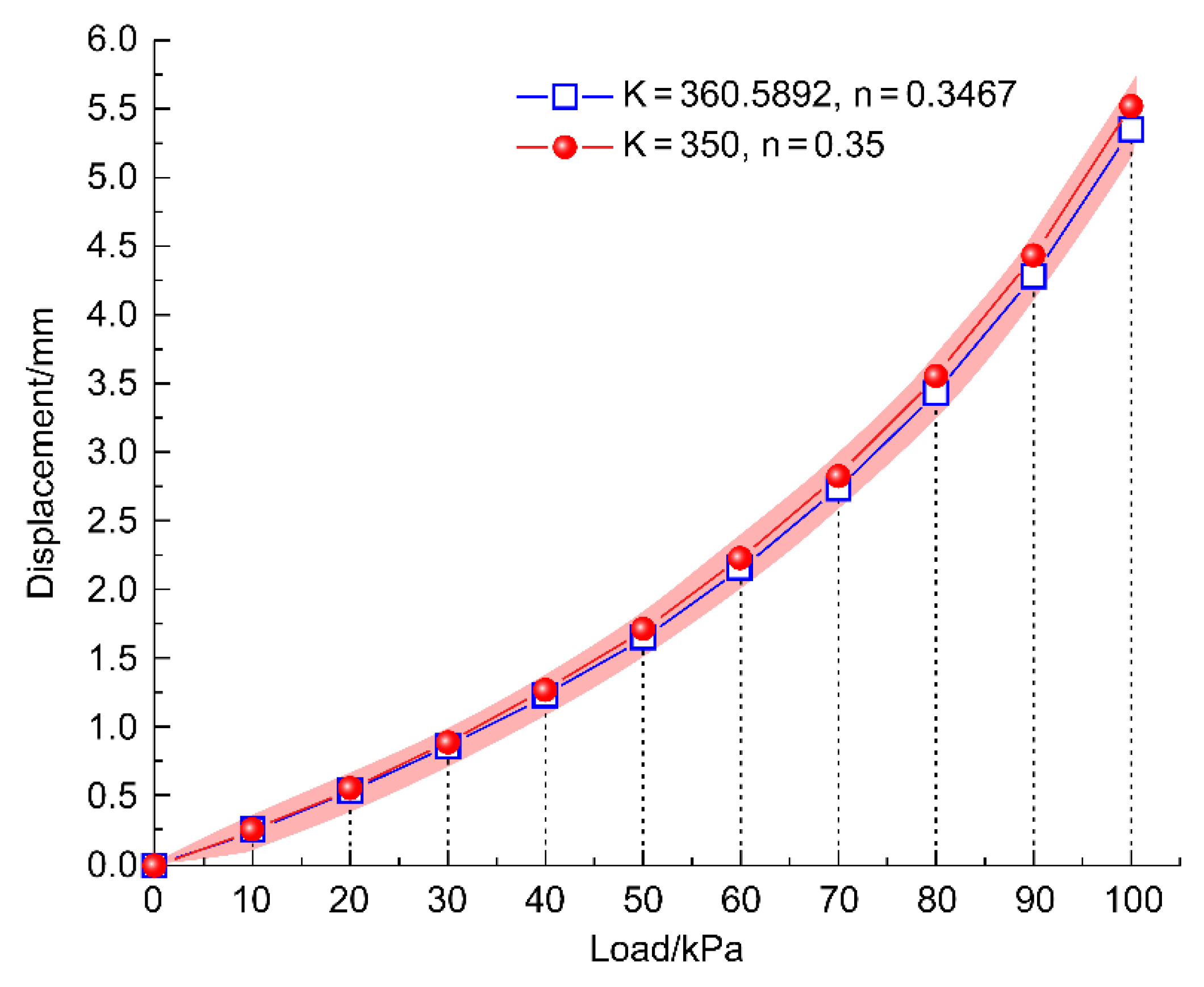
A collaborative optimization system integrating ABAQUS, Python, and MATLAB software was developed. In the context of self-test parameter inversion stability, parameter deviation did not exceed 5% of the preset value.

(2)

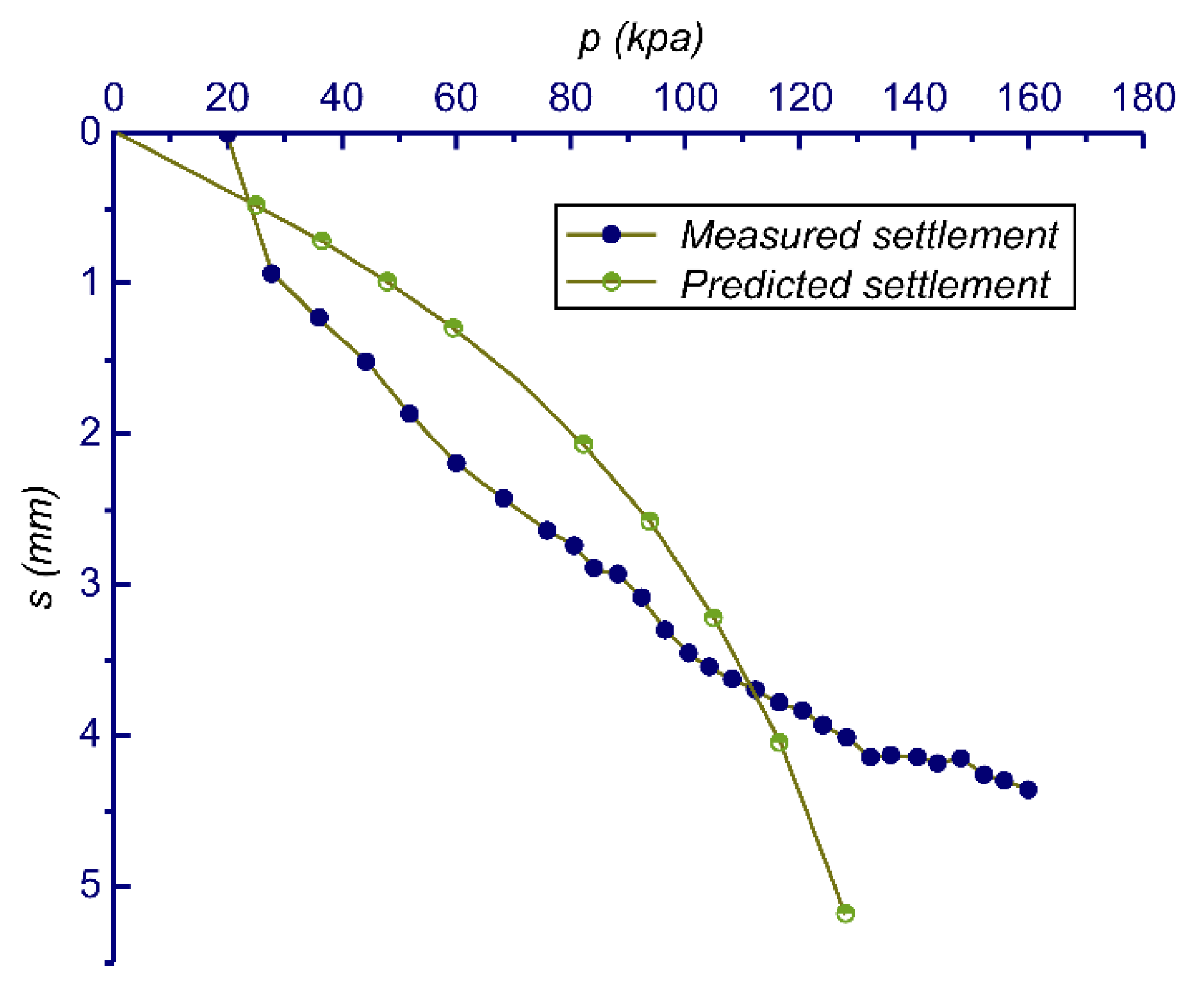
The experimental configuration, incorporating a 0.5 m × 0.5 m loading plate and inductive sensors, was used to generate pressure–settlement (p–s) curves. Through parameter inversion, the optimized DC model parameters were determined to be K = 401.40 and n = 0.55, with an MSE of 0.4773.

(3)

When the applied load exceeded 132 kPa, boundary effects significantly influenced the test results owing to local stress concentrations at the edges.

(4)

The DC constitutive model adopted herein characterizes the soil as a nonlinear model. Although the DC model can reasonably predict nonlinear elastic deformation, it inherently lacks accuracy in capturing complex plastic deformation or localized shear behaviors, exhibiting limitations under high-loading scenarios as the boundary effects intensify.

(5)

Such inherent locality constraints of the DC approach might pose challenges in accurately modeling more sophisticated engineering problems. In particular, with increasingly complex simulations in ABAQUS, computational demands will notably increase, implying the necessity for further improvements and refinements in future research.

(6)

The DC model exhibits good performance under the following conditions:

The constitutive framework of the DC model is simple and its parameters are easy to calibrate; thus, it is widely applied in geotechnical engineering.

When conducting parameter inversion based on load–settlement (p–s) curves from shallow plate load tests, the DC model can well represent the general characteristics and accurately reproduce the measured curves, effectively supporting engineering design under moderate-loading conditions without significant boundary effects.

This study presents a practical procedure: prior to structural construction, data obtained from field loading tests are combined with optimization algorithms to identify nonlinear constitutive parameters of soils. These identified parameters then facilitate precise predictions of the actual foundation behaviors.

For existing structural foundations, the method can rapidly invert soil constitutive parameters using a limited amount of plate loading test data, effectively predicting foundation settlement behaviors under extended loading scenarios.

While assessing slope stability, the method combines inversion-derived parameters with numerical calculations to evaluate slope stability more precisely, thus supporting stability assessments of slopes in engineering practice.

Regarding pavement design and subgrade assessments, the method facilitates the accurate prediction of deformation responses under traffic loading through parameter inversion, ensuring reliable engineering designs of transportation infrastructure founded on homogeneous soils.

For cohesive soil regions, inversion results can guide adjustments of the supporting structure stiffness, helping avoid excessive settlement.

(7)

The proposed method has the following limitations:

Original tests, such as the plate loading tests conducted in this study, generally represent common engineering observational scenarios. However, when applied to situations involving complex boundary conditions or substantial foundation load testing, the accuracy and reliability decrease owing to the inherent constraints of the DC model. Specifically, limitations arise owing to increased computational demands and complexity, potentially requiring significantly enhanced computational resources. The DC model’s sensitivity to boundary effects may cause discrepancies between the predictions and actual results under high-stress conditions.

(8)

If the DC constitutive model is replaced with more complex elastoplastic models, such as the modified Cam–Clay model, in future research, the increased number of parameters and computational complexity will present challenges. Further algorithmic improvements and refinements are thus necessary.

In summary, the collaborative optimization framework integrating ABAQUS, Python, and MATLAB developed in this study effectively addresses numerical stability and parameter identification accuracy. Although the DC model proved reliable under moderate loading and minimal boundary effects, further enhancements and validations are required to extend its applicability to more complex geotechnical scenarios involving significant boundary effects or substantial plastic deformation.

References

1. Anderson, J.B.; Townsend, F.C.; Rahelison, L. Load testing and settlement prediction of shallow foundation. J. Geotech. Geoenviron. Eng. 2007, 133, 1494–1502. [Google Scholar] [CrossRef]
2. Coduto, D.P.; Kitch, W.A.; Yeung, M.R. Foundation Design: Principles and Practices, 3rd ed.; Pearson: Boston, MA, USA, 2016; ISBN 978-0-13-341189-8. [Google Scholar]
3. GB 50007-2011; Code for Design of Building Foundation. Architecture & Building Press: Beijing, China, 2011.
4. Bray, J.D.; Macedo, J. 6th Ishihara Lecture: Simplified Procedure for Estimating Liquefaction-Induced Building Settlement. Soil Dyn. Earthq. Eng. 2017, 102, 215–231. [Google Scholar] [CrossRef]
5. Cho, G.-C.; Dodds, J.; Santamarina, J.C. Particle shape effects on packing density, stiffness, and strength: Natural and crushed sands. J. Geotech. Geoenviron. Eng. 2006, 132, 591–602. [Google Scholar] [CrossRef]
6. Chang, C.S.; Duncan, J.M. Consolidation analysis for partly saturated clay by using an elastic–plastic effective stress–strain model. Int. J. Numer. Anal. Methods Geomech. 1983, 7, 39–55. [Google Scholar] [CrossRef]
7. Chen, C.L.; Shao, S.J.; Ma, L. Duncan-Chang nonlinear elastic model considered loess structure. Appl. Mech. Mater. 2011, 90–93, 176–181. [Google Scholar] [CrossRef]
8. Zhang, L.; Chen, Y.; Liu, X.; Wei, X. A unified monotonic model for sand based on modified hyperbolic equation and state-dependent dilatancy. Comput. Geotech. 2020, 128, 103788. [Google Scholar] [CrossRef]
9. Dong, W.; Hu, L.; Yu, Y.Z.; Lv, H. Comparison between Duncan and Chang’s EB model and the generalized plasticity model in the analysis of a high earth-rockfill dam. J. Appl. Math. 2013, 2013, 709430. [Google Scholar] [CrossRef]
10. Dong, L.; Wu, N.; Zhang, Y.; Liao, H.; Hu, G.; Li, Y. Improved Duncan-Chang model for reconstituted hydrate-bearing clayey silt from the South China Sea. Adv. Geo-Energy Res. 2023, 8, 136–140. [Google Scholar] [CrossRef]
11. Cai, X.; Zhang, Y.; Guo, X.; Liu, Q.; Zhang, X.; Xie, X. Functional zoning optimization design of cemented sand and gravel dam based on modified Duncan-Chang nonlinear elastic model. Case Stud. Constr. Mater. 2022, 17, e01511. [Google Scholar] [CrossRef]
12. Wang, W.; He, P.; Zhao, B.; Hu, A.; Shang, J. Application of Duncan-Chang model on the numerical analysis considering the clay heterogeneity. In Proceedings of GeoShanghai 2018 International Conference: Fundamentals of Soil Behaviours; Zhou, A., Tao, J., Gu, X., Hu, L., Eds.; Springer: Singapore, 2018; pp. 929–937. [Google Scholar]
13. Dai, Z.P.; Zhao, C.; Zhao, C.F. The development and implementation of improved Duncan-Chang constitutive model in ABAQUS. Appl. Mech. Mater. 2011, 99–100, 965–971. [Google Scholar] [CrossRef]
14. Guan, Q.Z.; Yang, Z.X.; Guo, N.; Hu, Z. Finite element geotechnical analysis incorporating deep learning-based soil model. Comput. Geotech. 2023, 154, 105120. [Google Scholar] [CrossRef]
15. Wan, J.; Jiang, S.; Li, X.; Chang, Z. Development of improved finite element formulations for pile group behavior analysis under cyclic loading. Int. J. Numer. Anal. Methods Geomech. 2024, 48, 4089–4109. [Google Scholar] [CrossRef]
16. Ghorbani, J.; Aghdasi, S.; Nazem, M.; McCartney, J.S.; Kodikara, J. Parameters in play: AlphaZero-inspired AI for autonomous parameter identification in soil constitutive and finite element models. Comput. Geotech. 2024, 174, 106657. [Google Scholar] [CrossRef]
17. Erayman, E.; Yildiz, M.; Çavuş, U.Ş.; Yildiz, A. Finite element solution of dim dam under static loading using Duncan–Chang modelling. Online J. Sci. Technol. 2016, 6, 42–48. [Google Scholar]
18. MolaAbasi, H.; Saberian, M.; Khajeh, A.; Li, J.; Jamshidi Chenari, R. Settlement predictions of shallow foundations for non-cohesive soils based on CPT records-polynomial model. Comput. Geotech. 2020, 128, 103811. [Google Scholar] [CrossRef]
19. Fattahi, H.; Ghaedi, H. Improving accuracy in shallow foundation settlement prediction using rock engineering system method. Indian Geotech. J. 2024. [Google Scholar] [CrossRef]
20. Hu, A.-F.; Xie, S.-L.; Li, T.; Xiao, Z.-R.; Chen, Y.; Chen, Y.-Y. Soil parameter inversion modeling using deep learning algorithms and its application to settlement prediction: A comparative study. Acta Geotech. 2023, 18, 5597–5618. [Google Scholar] [CrossRef]
21. Singh, A.; Mitchell, J.K. General stress-strain-time function for soils. J. Soil Mech. Found. Div. 1968, 94, 21–46. [Google Scholar] [CrossRef]
22. Asgarkhani, N.; Kazemi, F.; Jankowski, R. Machine learning-based prediction of residual drift and seismic risk assessment of steel moment-resisting frames considering soil-structure interaction. Comput. Struct. 2023, 289, 107181. [Google Scholar] [CrossRef]
23. He, B.-H.; Du, X.-L.; Bai, M.-Z.; Yang, J.-W.; Ma, D. Inverse analysis of geotechnical parameters using an improved version of non-dominated sorting genetic algorithm II. Comput. Geotech. 2024, 171, 106416. [Google Scholar] [CrossRef]
24. ISO 22477-2:2015; Geotechnical Investigation and Testing—Field Testing—Part 2: Static Load Testing of Piles. International Organization for Standardization: Geneva, Switzerland, 2015.
25. Ji, Y.; Zuo, S.; Zhang, J.; Zhang, Y. Modified Duncan-Chang Model and Mechanics Parameter Determination Based on Triaxial Consolidated Drained Tests of Guiyang Red Clay in China. In New Solutions for Challenges in Applications of New Materials and Geotechnical Issues; Wang, S., Xinbao, Y., Tefe, M., Eds.; Springer International Publishing: Hangzhou, China, 2019; pp. 1–17. [Google Scholar]
26. Peng, W.; Wang, Q.; Liu, Y.; Sun, X.; Chen, Y.; Han, M. The influence of freeze-thaw cycles on the mechanical properties and parameters of the Duncan-chang constitutive model of remolded Saline Soil in Nong’an County, Jilin Province, Northeastern China. Appl. Sci. 2019, 9, 4941. [Google Scholar] [CrossRef]
27. Yan, M.; Yan, R.; Yu, H. Strain-softening characteristics of hydrate-bearing sediments and modified Duncan–Chang Model. Adv. Mater. Sci. Eng. 2021, 2021, 2809370. [Google Scholar] [CrossRef]
28. Tang, B.; Liu, T.; Zhou, B. Duncan–Chang E-υ Model Considering the thixotropy of clay in the Zhanjiang formation. Sustainability 2022, 14, 12258. [Google Scholar] [CrossRef]
29. Lang, M.; Deng, C. Comparative Analysis of Duncan-Zhang E-ν and E-B Models. In Proceedings of the 2021 3rd International Academic Exchange Conference on Science and Technology Innovation (IAECST), Guangzhou, China, 10 December 2021; pp. 2008–2011. [Google Scholar]
30. Ali, R.; Mounir, G.; Moncef, T. Adaptive probabilities of crossover and mutation in genetic algorithm for solving stochastic vehicle routing problem. Int. J. Adv. Intell. Paradig. 2016, 8, 318. [Google Scholar] [CrossRef]
31. Liu, Y.; Zheng, Y. Plastic Mechanics of Geomaterial; Springer: Singapore, 2019. [Google Scholar]
32. Deep, K.; Bansal, J.C. Optimization of Directional Overcurrent Relay Times Using Laplace Crossover Particle Swarm Optimization (LXPSO). In Proceedings of the 2009 World Congress on Nature & Biologically Inspired Computing (NaBIC), Coimbatore, India, 9–11 December 2009; pp. 288–293. [Google Scholar] [CrossRef]
33. Wang, G.; Yang, C.; Ma, X. A Novel Robust Nonlinear Kalman Filter Based on Multivariate Laplace Distribution. IEEE Trans. Circuits Sys. II Express Briefs 2021, 68, 2705–2709. [Google Scholar] [CrossRef]
Figure 1. (a) Square flexible bearing plate and (b) inductive displacement sensor.
Buildings 15 01108 g001
Figure 2. Calibration of the inductive displacement sensor. 1—millimeter; 2—extension rod; 3—stainless steel base.
Buildings 15 01108 g002
Figure 3. Loading test process. (a) Placing of polytetrafluoroethylene membrane; (b) Placing of multilayer canvas; (c) Placing of pressure plate and water pressure plate; (d) Loading test.
Buildings 15 01108 g003
Figure 4. Measured settlement ps curve.
Buildings 15 01108 g004
Figure 5. Triaxial test model.
Buildings 15 01108 g005
Figure 6. Curve of deviation stress versus axial strain.
Buildings 15 01108 g006
Figure 7. Flowchart of joint optimization method.
Buildings 15 01108 g007
Figure 8. FEM of indoor flexible bearing plate load test.
Buildings 15 01108 g008
Figure 9. Comparison of inversion curves.
Buildings 15 01108 g009
Figure 10. Comparison diagram of integration methods between C3D8 and C3D8R elements.
Buildings 15 01108 g010
Figure 11. Hourglass effect comparison.
Buildings 15 01108 g011
Figure 12. Comparison of ps curves for different grid sizes.
Buildings 15 01108 g012
Figure 13. FEM based on experiments.
Buildings 15 01108 g013
Figure 14. Comparison of predicted and measured settlement.
Buildings 15 01108 g014
Disclaimer/Publisher’s Note: The statements, opinions and data contained in all publications are solely those of the individual author(s) and contributor(s) and not of MDPI and/or the editor(s). MDPI and/or the editor(s) disclaim responsibility for any injury to people or property resulting from any ideas, methods, instructions or products referred to in the content.