Abstract
This paper constructs a theoretical framework integrating health risk transmission, remote work constraints, and spatial equilibrium to analyze the impact mechanisms of major public health events on the real estate market. This study finds that pandemics affect market equilibrium through multiple channels, including changes in residents’ utility functions, the reshaping of labor market structures, and adjustments in location choices. The model combines the SIR model from epidemiology with spatial economics to depict the endogenous decision mechanism of health risks. By constructing a two-sector general equilibrium model that includes remote work sectors, this study reveals the impact of technological change on the spatial structure of the real estate market. Based on the mobility preference theory, an asset pricing framework incorporating health risk premiums is established. Comparative static analysis shows that the health risk transmission coefficient influences housing prices through two channels: directly lowering willingness to pay and indirectly affecting the distribution of population density. Dynamic analysis indicates that, under specific parameter conditions, the market exhibits asymptotic stability. Policy simulation results show that the transmission effects of monetary and fiscal policies exhibit significant spatial heterogeneity, requiring policymakers to pay more attention to regional differences. This study not only enriches the analytical tools of real estate economics but also provides theoretical support for relevant policy formulation.
1. Introduction
The COVID-19 pandemic, as a major exogenous shock, provides a unique theoretical perspective for revisiting the price formation mechanism, spatial equilibrium theory, and asset pricing models in the real estate market (Gormsen & Koijen, 2020 [1]; Ye, 2016 [2]; Mo et al., 2023 [3]). Traditional real estate economics primarily focuses on the impact of fundamental factors like income and interest rates on market equilibrium (Giglio et al., 2021 [4]; Gupta et al., 2010 [5]; Preece et al., 2023 [6]). However, under the impact of significant public health events, the role of external factors such as health risks and spatial distance lacks systematic theoretical analysis (Wei & Liu, 2022 [7]; Caballero et al., 2021 [8]). This theoretical gap not only limits our understanding of the current trends in the real estate market but also hinders the improvement and innovation of related policy tools (Zhou et al., 2021 [9]; Yu et al., 2023 [10]).
We define several key concepts that are fundamental to our theoretical framework. “Health risk premium” refers to the additional return required by investors to compensate for the perceived health-related risks during pandemic periods, which directly affects asset pricing through changes in risk preferences and liquidity constraints. “Spatial equilibrium” describes a state where accounting for differences in amenities, prices, and health risks across locations, households and firms have no incentive to relocate, leading to a stable distribution of economic activities and population across space. This equilibrium is significantly altered during pandemic periods as health risks create new trade-offs in residential and workplace location decisions. Understanding these concepts is essential for analyzing how pandemic shocks restructure real estate markets through changes in risk assessment, spatial preferences, and the adoption of remote work technologies.
The existing literature on the impact of sudden events on asset prices is mainly based on utility maximization frameworks, incorporating risk premium terms to describe market responses (Campbell & Cochrane, 1999 [11]; Nazemi et al., 2024 [12]). However, such models often treat risks as exogenously given and fail to capture the endogenous evolution of factors like health risks and population mobility (Pedersen, 2022 [13]; Wan et al., 2021 [14]). At the same time, new working models such as remote work challenge traditional spatial equilibrium theories regarding the relationship between work and housing (Ehlert, 2021 [15]; Gao et al., 2023 [16]; Øvrelid et al., 2019 [17]). These theoretical dilemmas highlight the need for constructing a new analytical framework.
This paper aims to construct a unified theoretical framework based on general equilibrium theory by introducing elements such as a spatial transmission equation for health risks, distance-based labor market constraints for remote work, and liquidity preference in asset markets (Lorenz et al., 2023 [18]; Song et al., 2021 [19]; Rana et al., 2024 [20]). Specifically, the theoretical innovations in this paper are reflected in three main aspects:
First, by combining the SIR model from epidemiology with the location choice theory in spatial economics, we establish an endogenous decision-making mechanism for health risks (Moscone et al., 2014 [21]; Gu et al., 2020 [22]). By solving the utility maximization problem of representative agents under infection risk constraints, we derive the equilibrium relationship between health risks, population density, and housing prices (Merton, 1973 [23]; Kholodilin et al., 2020 [24]). This theoretical extension enriches the microfoundations of traditional real estate pricing models.
Second, we construct a two-sector general equilibrium model that includes a remote work sector to analyze the impact of labor market structural changes on real estate spatial equilibrium (Alonso, 1964 [25]; Mills, 1967 [26]; Ch et al., 2021 [27]). The model incorporates differentiated commuting cost functions to characterize the endogenous relationship between the proportion of remote work and location choice, providing a theoretical basis for explaining real estate market differentiation during the pandemic.
Third, based on liquidity preference theory, we establish an asset pricing framework that includes health risk premiums (Costola et al., 2023 [28]; Shiller, 2020 [29]). By incorporating the interaction between health risks and liquidity preferences, the model is able to explain certain paradoxical phenomena observed in the real estate market during the pandemic, such as price deviations from fundamentals in some regions.
The establishment of this theoretical framework not only helps us gain deeper insights into the operational patterns of the real estate market under pandemic shocks but also provides a theoretical foundation for designing related policy tools (Chernick et al., 2023 [30]; de La Paz et al., 2023 [31]; Stieglitz et al., 2013 [32]). Our analysis suggests that under significant public health events, traditional demand management policies may need to be differentially adjusted based on the spatial distribution characteristics of health risks (He et al., 2020 [33]; Benhabib et al., 2011 [34]). At the same time, the development of new employment models such as remote work requires policymakers to adopt more forward-looking measures in spatial planning and real estate regulation (Glaeser et al., 2005 [4]; Sun et al., 2023 [35]).
2. Literature Review
The development of health risks and asset pricing theory can be traced back to traditional asset pricing models. Early research focused primarily on how to incorporate external risk factors into pricing models, providing a fundamental analytical framework for understanding the impact of health risks on asset prices (Merton, 1973 [23]; Campbell & Cochrane, 1999 [11]). In the context of pandemics, academic discussions have delved deeper into the unique characteristics of health risks and their pricing effects. A large body of empirical research has found that health risks not only influence market expectations but also significantly heighten investors’ attention to tail risks.
Recent research has made important breakthroughs in model frameworks, particularly in attempting to integrate epidemiological models with asset pricing theory. In particular, scholars have found that the spatial diffusion characteristics of health risks can effectively explain the cross-sectional differences in asset prices when embedding the SIR model into a general equilibrium framework. At the same time, behavioral finance perspectives have provided new insights into the impact of health risks on investor behavior. These studies suggest that health risks not only alter investors’ risk preferences but also influence their investment decisions through attention allocation mechanisms (Kang et al., 2021 [36]; Ataullah et al., 2022 [37]; Alam et al., 2021 [38]; Walby et al., 2016 [39]).
In the area of panic sentiment contagion, recent scholars have achieved fruitful results through diverse research methods. The rise in social media has provided a new perspective for studying market sentiment, with studies showing that the information dissemination mechanism significantly accelerates the market panic spread (Hirshleifer et al., 2021 [40]; Lim et al., 2021 [41]). Notably, during crises, the spatial correlation of market sentiment exhibits a significant strengthening trend. Some pioneering studies have explored the physiological basis of panic emotions from a neuroscience perspective, finding that health risk-related news reports trigger risk-averse behavior among investors (Kang et al., 2020 [42]). These findings provide a deeper understanding of the formation mechanisms of market sentiment.
In terms of identifying the impact of sentiment contagion on asset prices, recent studies have adopted more rigorous empirical strategies. By comparing similar regions with different social network connectivity, researchers found that sentiment contagion explained a significant portion of housing price synchronization during the pandemic (Ho et al., 2024 [43]; Jiang et al., 2024 [44]). More in-depth theoretical studies have introduced social learning theory into asset pricing models, analyzing the diffusion mechanism of panic emotions under incomplete information environments and constructing general equilibrium models with heterogeneous beliefs to explain the dynamic evolution of market participants’ expectations (Bikhchandani et al., 2024 [45]; Brunnermeier et al., 2021 [46]).
The development of spatial economics theory reflects academia’s ongoing attention to emerging technological changes. With the widespread adoption of remote work technology, researchers have expanded traditional monocentric city models (Ehlert, 2021 [15]; Haefner et al., 2020 [47]). Empirical studies using big data methods have recorded the spatial restructuring of office activities during the pandemic, finding significant differentiation in housing prices between commercial and residential areas (Yang et al., 2023 [48]). In cities with higher remote work friendliness, suburban housing prices exhibited more pronounced appreciation trends (Choudhury et al., 2021 [49]; Henderson et al., 2021 [50]).
In the study of policy transmission mechanisms, the recent literature has increasingly focused on the spatial heterogeneity characteristics. Cross-regional studies have found that the impact of interest rate changes on housing prices varies significantly by region, mainly due to differences in the development levels of local financial markets (Gupta et al., 2010 [5]; Liu et al., 2022 [51]). Research on fiscal policy has focused on comparing the effects of different policy tools, finding that infrastructure investment has stronger spatial spillover effects compared to tax incentives (Deng et al., 2023 [52]; Lima, 2020 [53]). Recent systematic reviews and empirical studies further support these findings, with Di Liddo et al. (2023) [54] documenting emerging trends in real estate market dynamics following COVID-19 and Holmgren Bentzer (2024) [55] providing evidence on the persistent transformation of office vacancy patterns in Stockholm as an indicator of the “new normal” in commercial real estate markets.
At the policy coordination level, scholars have paid more attention to the interaction between monetary and fiscal policies. By constructing a DSGE model with heterogeneous agents, studies have found that the optimal policy mix varies according to the spatial characteristics of income distribution (Baccini et al., 2024 [56]; Tian et al., 2017 [57]). Methodological innovations, such as machine learning methods and spatial effect decomposition using high-dimensional panel data, have provided new tools for identifying policy effects (Calainho et al., 2024 [58]; Jarrow et al., 2022 [41]).
Firstly, while some research has started to focus on the impact of health risks on asset pricing, most studies still treat the pandemic shock as an exogenous variable, neglecting the endogenous interactions between health risks, market sentiment, and spatial structure. Although empirical studies have documented the pricing effects of health risks, they have failed to reveal the micro-mechanisms of risk transmission (He & Xia, 2020 [59]). Secondly, regarding the spatial contagion characteristics of panic sentiment, existing studies tend to focus on correlation analysis using network data, lacking an in-depth understanding of the contagion mechanism (Meyfroidt et al., 2022 [60]). Thirdly, research on the impact of remote work on spatial structure has rarely considered the moderating effect of health risks, making it difficult to fully explain the asymmetric adjustment phenomena observed during the pandemic. Finally, in exploring the spatial heterogeneity of policy effects, existing research often overlooks the impact of health risk distribution on policy transmission.
Based on the above understanding, this paper proposes a unified theoretical framework with the following three major innovations: First, by integrating the SIR model with asset pricing theory and introducing a dynamic health risk equation with a spatial diffusion term, it enables the endogenous treatment of the risk transmission mechanism. This innovation overcomes the limitation of existing research that treats the pandemic shock as an exogenous impact, allowing the model to better explain the dynamic interaction between risks and prices (Lim et al., 2021 [61]). Second, this paper constructs a behavioral finance model that considers the spatial contagion of panic sentiment, using a social network structure to design an emotion diffusion equation. This provides new explanations for understanding irrational market responses during the pandemic. Third, it introduces health risk constraints into the classic spatial equilibrium framework, analyzing how the distribution of risks influences remote work decisions and location choices. This enriches the traditional theory and reveals the interactive effects of technological change and health risks in reshaping urban spatial structure (Muth, 1969 [62]).
The theoretical scope of this study focuses primarily on the dynamic mechanisms of real estate markets under pandemic conditions, particularly by integrating epidemiological models with spatial economics principles to explore the endogenous interactions among health risks, remote work, and asset pricing. The research framework encompasses not only micro-level individual decision-making behaviors but also extends to macro-policy transmission and spatial equilibrium analysis, providing a comprehensive theoretical explanation system for the real estate market in the post-pandemic era. The application range of this framework includes, but is not limited to, urban planning policy formulation, real estate regulatory measure evaluation, and macroeconomic policy effect analysis.
Figure 1 presents the theoretical framework constructed in this paper and its underlying mechanisms. The framework centers on the equilibrium of the real estate market and depicts the market operation mechanism under pandemic impact through three transmission levels. At the upper level, the SIR transmission model describes the spatial diffusion process of health risks, which affects population density , thereby altering the remote work equilibrium and labor market structure . At the central level, these factors jointly determine the equilibrium price of the real estate market, considering not only traditional income and commuting costs but also the discounting effect of health risks. At the lower level, the model outlines the triple feedback channels in the market: first, through the risk premium , which affects asset pricing; second, through policy transmission , which adjusts market operations; and third, through market sentiment and social welfare , reflecting the overall equilibrium state of the market. This theoretical framework not only unifies the mechanisms in the existing literature but also reveals the endogenous interactions between health risks, spatial structure, and market behavior, providing a systematic analytical tool for understanding the dynamics of the real estate market under pandemic impact. Notably, this framework highlights the following three innovative features: First, by combining the SIR model with spatial economics, it enables the endogenous treatment of the health risk transmission mechanism. Second, by introducing a differentiated commuting cost function, it portrays the reshaping effects of remote work on spatial structure. Finally, through constructing an asset pricing framework that includes health risk premiums, it reveals how health-related uncertainties reshape asset valuation and investor behavior.

Figure 1.
Theoretical framework of the real estate market under pandemic impact.
3. Theoretical Framework and Model Construction
3.1. Basic Model Setup
This study examines an economic system with continuous spatial distribution characteristics, where represents the spatial location index. The core idea of this setup is to continue the spatial dimension, allowing the analysis to cover diverse spatial structures such as the central business district (CBD), sub-center areas, and more remote suburban regions. In a typical urban structure before the pandemic, CBDs usually have high population density, concentrated public facilities and services, and high rent and land prices. With the deep and widespread impact of the pandemic, people’s demand for spatial dispersion, low-density residential environments, and remote work has become increasingly prominent, driving urban spatial structures to begin to expand from the center outwards. The continuous spatial setting of this model naturally accommodates such phenomena and provides a theoretical foundation for analyzing the impact of “dispersed housing” and “remote work” on the traditional spatial structure during the pandemic.
At each location , there are three main economic agents: representative households, real estate developers, and the government. Households decide the allocation between housing and general consumption goods while facing the dual considerations of health risk and commuting costs; real estate developers influence the regional housing price structure through the construction and supply of housing in different locations; and the government influences the asset price dynamics and the transmission path of health risks across regions through monetary and fiscal policies. The interaction between these economic agents forms an endogenous equilibrium at the spatial scale, enabling the model to explore the chain effects of the pandemic on urban spatial structure and asset pricing.
3.1.1. Representative Household Behavior Model
During the pandemic, household decision making is significantly influenced by health risks. To capture this feature, we set the following utility function for the representative household at location :
where represents the housing service consumption at location is the consumption of general goods, and is the health risk level of the region. The parameter measures the relative importance of housing services in total utility. Due to the pandemic-induced home isolation and social distancing measures, households’ demand for living space significantly increases, and thus, may increase during the pandemic. The parameter represents the risk aversion coefficient, which describes the utility loss households experience when facing health risks. This coefficient may vary across regions, for instance, households in areas with a higher elderly population or insufficient healthcare resources may be more sensitive to health risks.
The budget constraint faced by households at location is
where is the price of housing at location is the local wage level, is the commuting cost coefficient, is the commuting distance, and represents the proportion of the household in region that engages in remote work. The detailed derivation of the household’s optimization problem is presented in Appendix A. This budget constraint considers three key factors during the pandemic:
Housing price fluctuations: With the pandemic-induced shift in spatial demand, housing prices may differ across regions due to changes in households’ demand for living space. As remote work increases, households’ location choices become more flexible, and the growing demand for more remote areas may lead to price increases in those regions.
A reduction in commuting costs: With the widespread adoption of remote work, household income structures change. As the proportion of remote work increases, households no longer need to bear commuting-related costs . Therefore, the higher the proportion of remote work, the smaller the impact of commuting costs on the household’s budget, thus increasing disposable income.
Changes in spatial structure: The popularization of remote work changes traditional working models, influencing household choices in residential areas. When (complete remote work), households no longer need to consider commuting distances. The budget constraint simplifies to , meaning the entire wage is available without being affected by commuting costs, making more distant areas attractive.
By solving the household utility maximization problem, we can derive the demand for housing services and general goods and further analyze the spatial distribution sensitivity of housing prices, wages, and commuting costs. These results will provide the theoretical foundation for subsequent spatial equilibrium analysis, helping us understand the far-reaching effects of the pandemic on the real estate market and household behavior.
3.1.2. Health Risk Spatial Transmission Mechanism
To describe the transmission dynamics of the pandemic across space, we introduce elements from the epidemiological SIR model. Here, we focus on the evolution of the health risk status (such as infection rates or infection risk indicators), with the dynamic equation given by
This dynamic equation incorporates two types of transmission mechanisms: First is the local transmission effect , where is the local infection rate and is the population density at location . Densely populated areas typically have higher transmission intensities, which explains why high-density areas are more severely affected during the initial stages of an outbreak. Second is the cross-region transmission effect , where describes the intensity of cross-region transmission, and is the spatial weight kernel function, representing the degree of population movement or interaction between locations and . This setup helps explain the “risk diffusion” phenomenon during the pandemic, where people may migrate from high-risk areas to low-density regions, but this also causes risk spillovers across regions.
Figure 2 presents the dynamic diffusion of risk in a social network in terms of nodes and edges, with the color intensity reflecting the level of risk (darker colors represent higher risks). Over time (from to ), high-risk nodes gradually transmit the risk to other nodes through the network structure. The network density and risk distribution change significantly, helping to understand the social transmission mechanisms of emotions and risks during the pandemic. Through this risk transmission mechanism, we incorporate health risks into the spatial dimension of the study, providing the foundation for analyzing the interaction between spatial structures and economic decisions (such as housing choices and remote work arrangements).
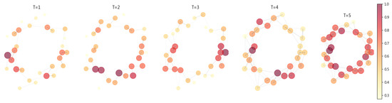
Figure 2.
Network density dynamic evolution.
3.2. Equilibrium Analysis of Remote Work
3.2.1. The Binary Structure of the Labor Market
The pandemic highlighted the significant differences in the feasibility and flexibility of remote work across industries. We divide the economy into two sectors: the remote work (T-type) sector and the non-remote work (NT-type) sector. The T-type sector, including financial services, technological research and development, and information transmission, is characterized by the ability to complete work tasks via online platforms. The NT-type sector, such as manufacturing, logistics, transportation, and retail services, requires physical presence or on-site operations.
The total output function can be represented as
where and are the production efficiency parameters of the two sectors, and and are the output elasticities. and represent the labor inputs in the remote work and non-remote work sectors, respectively. This setup suggests that an increase in the proportion of remote work (via an increase in ) will influence the output structure and reshape the characteristics of the labor market. Additionally, can be used to represent digital infrastructure and technological proficiency. When the level of digitization is high, the marginal return on labor input in the T-type sector is higher, which promotes an increase in the proportion of remote work.
3.2.2. The Determination of the Proportion of Remote Work
In a given region , firms face the decision of how to allocate labor between the remote work (T-type) sector and the non-remote work (NT-type) sector. To simplify the analysis, we assume that the total labor is fixed, and the firm’s decision variable is the proportion of remote work , which represents the proportion of labor allocated to the T-type sector. Based on the modified household budget constraint, firms must maximize output while considering changes in labor cost structures. Especially with the combination of remote work and traditional work models, labor costs and productivity will differ. Therefore, the firm’s objective function can be expressed as
In this equation, and are the production efficiency parameters for the remote work (T-type) and non-remote work (NT-type) sectors, respectively; is the local wage level; is the commuting cost coefficient; is the commuting distance; is the proportion of remote work; and is the proportion of traditional work. This model considers two main factors. The Impact of Remote Work on Labor Costs: When firms decide to shift labor toward remote work, the wages paid to employees may not change, but remote work eliminates commuting costs. For traditional work , firms must pay wages adjusted for commuting costs . Therefore, remote work alters the labor cost structure, particularly in regions with high commuting costs, where the relative advantage of remote work increases.
Productivity and Technological Factors: The proportion of remote work also depends on the technological parameters of the T-type and NT-type sectors. When digital infrastructure is well developed and online collaboration efficiency is high, remote work (in the T-type sector) becomes more attractive, increasing . Therefore, firms adjust their labor allocation based on technological conditions and productivity to optimize their production process.
By solving the first-order condition for , we can derive the equilibrium solution for the proportion of remote work:
This conclusion shows that the proportion of remote work depends not only on the technological parameters of the two sectors and but also on commuting costs . When the level of digitization is higher, the proportion of remote work increases, reflecting that improved digital infrastructure facilitates the expansion of remote work. Similarly, when commuting costs are high, the relative advantage of remote work strengthens, pushing upward.
This result helps explain the phenomenon of industrial differentiation during the pandemic: on the one hand, industries with higher levels of digitalization can more quickly adapt to remote work, making it easier to increase the proportion of remote work, and on the other hand, firms located in regions with high commuting costs (such as urban fringe or suburban areas) have more motivation to increase the proportion of remote work to reduce labor costs. This also explains why, in the post-pandemic era, the proportion of remote work may remain high due to structural reasons—not only because of technological factors but also because of spatial economic efficiency considerations. The promotion of remote work makes the trade-off between commuting costs and production modes more flexible and efficient.
3.2.3. Reconstruction of Spatial Equilibrium
After endogenizing the proportion of remote work and health risks, the equilibrium condition across locations requires that the utility levels of representative households in all locations be equal, i.e.,
By substituting the equilibrium demand quantities from the budget constraint and household utility function, we derive the equilibrium housing price expression, which can be simplified as follows:
This result integrates the key factors affecting housing prices into the same framework and reveals the mechanisms through which the pandemic impacts spatial price structures: First, health risks negatively affect housing prices through the function. Higher health risks in a region reduce housing demand, leading to lower prices. Second, the proportion of remote work reduces the impact of commuting costs on housing prices, making more remote areas and suburban regions more attractive after the pandemic. Finally, the wage level and industrial structure (implicitly reflected in and ) represent the economic vitality of a location, helping distinguish areas that can maintain strong housing prices and industrial structure advantages after the pandemic.
3.3. A Dynamic Extension of the Asset Pricing Framework
During the pandemic, market liquidity and investor risk preferences fluctuated significantly with changes in health risks, which not only affected capital markets but also had a profound impact on the real estate market. The rise in health risks typically leads to an increase in investor risk aversion, thereby altering the process of asset price formation. To capture these dynamic adjustments, we introduce a dynamic risk premium term in the traditional asset pricing model, which adjusts according to the health risk . The specific asset pricing model can be expressed as
where represents the real estate price at location is the expected total return on real estate in period (including rental income and capital appreciation); is the expectation operator conditioned on the information set at time is the risk-free rate; and is the risk premium function that reflects the non-linear impact of health risk on asset prices.
The Risk Premium Function and the Impact of Health Risks
The risk premium function takes into account how health risks during the pandemic influence market liquidity and investor risk preferences. Specifically, the risk premium function is expressed in a non-linear form as
where is the baseline risk premium, is the linear risk impact parameter capturing the direct effect of health risks on asset prices, and reflects the non-linear effects such as liquidity exhaustion or market mispricing that may occur in high-risk areas. This non-linear setup explains why asset prices in high-risk areas tend to fall more deeply during the peak of the pandemic and why market liquidity may contract non-linearly.
Next, we analyze the structure of the total return on assets and the impact of the pandemic. The expected total return can be further decomposed as
where rent i,t+1 is the expected rental income for period and is the expected property price in period . This return structure reflects the dual characteristics of real estate as an investment asset: on the one hand, real estate provides current rental income, and on the other, it offers potential capital appreciation. The impact of the pandemic not only influences asset returns by changing current rental levels but also alters investor expectations about future property prices, thereby affecting the overall return on assets.
For instance, in the early stages of the pandemic, due to a significant increase in health risks, rental levels in many areas may be suppressed, particularly in high-risk regions. This will lead investors to lower their expectations for future capital appreciation in these areas, thereby depressing property prices. As the pandemic progresses, the widespread adoption of remote work and the gradual decrease in health risks will restore investor confidence, possibly leading to a recovery in rental income and a rebound in property prices.
In addition to the direct impact of health risks, the perspective of spatial economics becomes particularly important during the pandemic. With the rise in remote work, the demand for location has changed significantly for both households and businesses. Certain areas, with lower commuting costs and higher residential comfort, have become more attractive. Property prices in these regions may show higher growth potential during the pandemic, altering the market’s pricing logic for assets. Furthermore, market liquidity is also an important factor to consider. In high-risk areas, due to the economic uncertainty triggered by the pandemic, investors may choose to reduce their holdings of risk assets, further exacerbating price declines in these regions. Conversely, in relatively low-risk areas, as market liquidity gradually recovers, real estate assets in these regions may show more stable growth.
The model and analytical framework presented above provide a theoretical foundation for asset pricing in the post-pandemic era. By incorporating health risks, the impact of remote work, and changes in market liquidity, we can better understand the dynamic adjustment mechanisms of asset prices. In practical applications, this model helps predict the performance of different industries and regions during the pandemic and provides valuable market guidance for investors. For example, investors can adjust their asset allocation strategies based on the dynamic changes in the risk premium function , thereby reducing potential risk exposure and seizing opportunities for market recovery.
While the baseline model assumes rational decision making, real-world pandemic responses often feature market panic and irrational behavior. To address this limitation, we extend our framework by incorporating behavioral elements through a sentiment contagion model with heterogeneous agents. We introduce a sentiment variable representing the deviation from rational expectations in location at time , which follows a modified Bass diffusion process with spatial properties:
where represents the direct impact of health risks on sentiment, captures social contagion intensity, is the social connectivity kernel between locations and measures price feedback effects, and is the sentiment decay rate reflecting gradual return to rationality.
With this sentiment variable, the asset pricing equation is modified to incorporate behavioral effects:
where represents the behaviorally biased expectation operator and is the sentiment premium function, specified as follows:
with and . This asymmetric specification captures the empirical observation that negative sentiment (panic) exerts a disproportionately larger impact on risk premiums than positive sentiment.
The behavioral expectation operator introduces bounded rationality through
where represents the weight on non-rational expectations , which follows an adaptive process based on recent price movements:
with being a non-linear transformation function capturing trend-chasing behavior and representing the lookback window.
In equilibrium, sentiment dynamics introduce multiple potential steady states. Defining the system state vector as , the fixed points satisfy
where is the system dynamics function. Under certain parameter configurations, this system admits multiple equilibria characterized by different sentiment regimes:
where represents the panic equilibrium with depressed prices, represents the rational expectation equilibrium, and represents the exuberance equilibrium.
Through bifurcation analysis, we find that the threshold for transitioning between equilibria depends on both the health risk level and the social connectivity structure:
When exceeds a critical threshold , the system can tip from the rational equilibrium into the panic regime, producing price dynamics that deviate substantially from fundamentals-based predictions. This insight helps explain why similar health risk levels can produce markedly different market outcomes across regions with different social structures or information environments.
The introduction of sentiment dynamics significantly enriches the model’s predictive capabilities, particularly in explaining the heightened volatility and apparent overreaction in housing markets during the initial phases of the pandemic. Moreover, it offers a theoretical foundation for understanding how non-pharmaceutical interventions like clear communication strategies might mitigate harmful sentiment contagion during public health crises.
3.4. Dynamic Adjustment Mechanism
3.4.1. Price Dynamics and Risk Evolution
To further analyze the linkage between asset prices and risks during the pandemic, we consider a dynamic system to describe the price adjustment and risk transmission:
In this system, describes the speed at which the price regresses toward its equilibrium level , with indicating that the market has a mean-reverting characteristic. The evolution mechanism of the health risk is consistent with the previously discussed SIR-type design. This dynamic system influences the asset price adjustment path through the spatial transmission of health risks, reflecting the spatial characteristics of severe price fluctuations in high-density areas during the early stages of the pandemic and a gradual stabilization of risks in the later stages. To better understand the spatial and temporal changes in price dynamics, Figure 3 presents a three-dimensional visualization of house prices across the spatial dimension and their evolution over time.
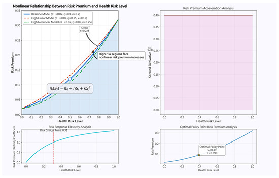
Figure 3.
System stability region diagram. Note: This figure presents a three-dimensional perspective showing the trajectory of house price indices changing with time and spatial locations. The color scale from dark to light corresponds to the levels of house prices, with the time axis displaying the price adjustment process from the early to late stages of the pandemic, highlighting the dynamic process where prices in high-risk areas drop rapidly in the early stage, followed by a gradual stabilization due to policy interventions and risk reduction.
3.4.2. System Stability Analysis
As shown in Figure 3, the stability of the system’s equilibrium state varies with different combinations of transmission coefficients () and price adjustment speeds (). The color transitions from cool to warm tones represent the system transitioning from a stable state to an unstable state. The left side of the diagram represents the stable region, while the right side represents the unstable region. This helps to understand the key conditions for market dynamic adjustments under the impact of the pandemic. By performing a local linearization analysis of the dynamic system, we can obtain its Jacobian matrix . A comprehensive mathematical analysis of the system’s stability and convergence properties is provided in Appendix A.7. The determination of stability depends on the eigenvalues of . In general, if the price adjusts sufficiently fast toward the equilibrium deviation and the local transmission rate is insufficient to maintain sustained infection (i.e., , leading to a weakening of cross-regional risk or gradual control), the system will exhibit local asymptotic stability. This stability result helps explain why, after an adjustment period, some regions can return to relatively stable price levels, while others may fall into long-term decline due to persistent high risks and asset value losses.
3.5. Policy Framework and Intervention Mechanism
3.5.1. Monetary Policy Response Function
During the pandemic, the central bank’s policy tools and response functions became particularly important. Suppose the central bank’s policy interest rate is set according to the standard Taylor rule:
where is the base interest rate, is the inflation rate, and are policy parameters, and is the potential output. During the pandemic, health risks may force the central bank to reassess the balance between price stability and economic stimulus. For example, in regions with extremely high health risks, monetary policy might encounter liquidity traps in high-risk assets, and the multiplier effect may be weak. At this point, and may vary with the risk level, leading to a non-linear response of monetary policy to regional economic conditions.
3.5.2. Fiscal Policy Framework
Similarly, the government can dynamically adjust fiscal expenditure in response to health risks and economic recovery needs:
where is the base public expenditure, is the average health risk level across regions, is the health risk response coefficient, and is the response to the output gap. During the pandemic, high-risk areas often require more significant fiscal support, such as the expansion of medical facilities, social protection measures, and subsidies. The response to fiscal stimulus in different regions is not uniform and may depend on the local industrial structure, infrastructure, and previous capital stock. The following figure (Figure 4) illustrates the evolution of network density over time, which can be viewed as the dynamic process through which risks gradually spread across regions.
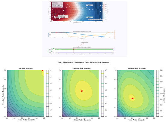
Figure 4.
Policy overlay effects under different risk scenarios.
3.5.3. Policy Coordination and Effect Evaluation
Ultimately, the coordination of monetary and fiscal policies affects the social welfare expression:
where represents the social cost of health risks. Policymakers must consider multiple objectives when formulating measures: in the short term, suppressing the pandemic, alleviating panic, and avoiding extreme asset market fluctuations; in the medium term, promoting industrial transformation and digital infrastructure development; and in the long term, guiding the urban spatial structure toward more resilient and adaptive adjustments through appropriate fiscal and monetary policy combinations. Due to spatial heterogeneity, industrial differentiation, and the non-linear characteristics of health risk transmission, policy effects will naturally vary between regions, meaning that differentiated and regionalized policy combinations may be better suited to the challenges of the post-pandemic era. By using monetary and fiscal policy intensities as the horizontal and vertical axes, Figure 3 displays the social welfare levels under various policy combinations. The figure presents the impact of different combinations of monetary policy (the horizontal axis) and fiscal policy (the vertical axis) intensities on social welfare in contour form. The color scale, from light to dark, corresponds to the improvement in welfare levels, with red stars marking the optimal policy combinations. This helps policymakers to develop better policy mixes in the pandemic context.
Through the above theoretical framework, this study integrates health risks, the expansion of remote work, spatial structure transformation, and policy transmission mechanisms within the same model. This framework not only helps explain the observed phenomena during the pandemic, such as the urban decentralization of residence, asset price differentiation, and industrial structure transformation, but also provides a theoretical foundation for future policy design. The spatial dimension considered in the model, dynamic adjustment mechanisms, and the flexible adjustment of policy parameters offer clear analytical paths and logical bases for empirical research and strategic formulation.
4. Model Equilibrium Analysis and Theoretical Implications
Based on the above theoretical framework, this section will delve into the equilibrium characteristics of the model and its underlying policy implications, aiming to reveal the profound impacts of the pandemic on the real estate market and the critical role played by government policies. First, we examine the existence and uniqueness of the model equilibrium, given the exogenous parameter set . The model equilibrium must simultaneously satisfy the utility maximization of the representative household, the profit maximization of developers, labor market clearing, spatial equilibrium, and the health risk steady state. Under basic assumptions such as the strict concavity of the utility function, diminishing returns to scale of the production function, and the continuity and boundedness of the spatial weight kernel function, we can construct the mapping from the bounded closed convex set , which contains all possible equilibrium variable combinations, to itself. By applying the Banach Fixed Point Theorem or the Brouwer–Tychonoff Fixed Point Theorem, we can prove the existence of an equilibrium solution. Furthermore, if the utility and production functions satisfy strict concavity, then the mapping possesses contraction properties, ensuring the uniqueness of the equilibrium solution according to the Contraction Mapping Theorem. This result suggests that, even in the context of pandemic shocks, the real estate market still has endogenous stabilization mechanisms that can clear the market and ensure the effective allocation of resources.
Based on the above theoretical framework, this section will further explore the equilibrium characteristics of the model and its underlying policy implications, aiming to reveal the profound impacts of the pandemic on the real estate market and the key role played by government policies. First, we will focus on the existence and uniqueness of the model equilibrium, which is based on the exogenous parameter set . According to the model setup, achieving an equilibrium solution requires satisfying a series of key conditions, including the utility maximization of the representative household, the profit maximization of developers, labor market clearing, spatial equilibrium, and the steady state of health risks. These conditions reflect the interactions of various economic agents in the market and ensure that, even when considering the pandemic shock, the market can still achieve an effective allocation of resources.
For the mathematical proof, we first analyze the properties of the utility function. Assuming the utility function is strictly concave, this guarantees that the representative household’s optimization problem has a unique solution. Specifically, the representative household will choose the optimal residential location and consumption structure based on the spatial structure, health risks, and labor market conditions. Next, the assumption of diminishing returns to scale in the production function ensures the optimal allocation of resources between different locations, further facilitating the existence of the equilibrium solution. The continuity and boundedness of the spatial weight kernel function ensure that the interregional interactions are mathematically manageable, which is crucial for simulating the spatial propagation of health risks.
Based on these assumptions, we define the feasible solution region , which contains all possible equilibrium variables. Specifically, the space is a set composed of the following variables:
These variables represent the price , consumption of general goods , consumption of housing services , health risk level , and proportion of remote work in each region. Due to the strict concavity of the utility function and the diminishing returns to scale of the production function, we can prove that is a bounded closed convex set. This conclusion guarantees that all equilibrium solutions lie within this range and ensures that no unrealistic solutions will emerge during numerical solutions. Next, we construct the mapping , which maps any element of space to the equilibrium solution in the next period. The mapping can be decomposed into several component functions, each corresponding to different economic behaviors and market constraints. Specifically, the mapping includes the following component functions:
- : Calculates the new equilibrium price based on the spatial equilibrium condition.
- : Updates consumption based on the household’s budget constraint.
- : Updates housing service consumption based on the household’s utility maximization problem.
- : Updates the risk level based on the health risk dynamic equation.
- : Calculates the remote work ratio based on the labor market equilibrium condition.
These component functions reflect the various economic interactions in the model and update the equilibrium variables at each time step. Specifically, adjusts the price based on the spatial equilibrium condition, while depends on the dynamic equation for the propagation of health risks to adjust the risk levels. These dynamic rules reflect the mutual influence between the real estate market and the labor market under pandemic shocks and help describe how the market achieves optimal resource allocation across different regions.
For the mapping , we can prove that it satisfies the contraction mapping condition, i.e., there exists a constant such that for any , we have
This contraction property arises from the boundedness of the marginal effects between each variable in the equilibrium process. Specifically, for each region , the marginal changes between price, consumption, housing service, health risk, and the remote work ratio are all bounded within a certain range, ensuring the contraction property of the mapping . This contraction property indicates that with multiple iterations, the model will gradually converge to a stable equilibrium solution.
According to the Contraction Mapping Theorem (Banach Fixed Point Theorem), the mapping has a unique fixed point , i.e., there exists a unique equilibrium solution such that
This result proves that, even under the impact of the pandemic, the real estate market can still achieve market clearing and that market resources will be effectively allocated under various economic parameter constraints. Furthermore, this result suggests that regardless of how strong the pandemic shock is, the market has endogenous stabilization mechanisms that can adjust prices and demand to ensure market equilibrium.
Additionally, we emphasize several key assumptions and conclusions in the model. First, the strict concavity of the utility function ensures that the representative household can make rational choices in response to health risks and labor market structure. Second, the diminishing returns to scale in the production function and the boundedness of the spatial weight kernel function ensure that interregional interactions are manageable and do not lead to excessive market fluctuations. Finally, the contraction property of the mapping guarantees the uniqueness of the equilibrium solution and provides a solid theoretical foundation for subsequent numerical simulations. To further illustrate the dynamic convergence toward equilibrium described by our model, Figure 5 depicts the iterative convergence process of housing prices across different risk-level regions under pandemic shocks, clearly confirming the theoretical stability discussed above.
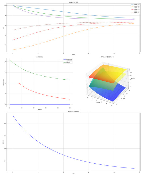
Figure 5.
Policy analysis diagram.
From the diagram, we observe that the blue solid line represents the price trajectory of low-risk areas, which shows a relatively smooth downward trend. The red dashed line indicates the price fluctuations in high-risk areas, which initially experience larger adjustments but stabilize afterward. The green line represents the price adjustments in medium-risk areas, which fall between the other two cases. These empirical observations strongly support the theoretical prediction that the market has an endogenous stabilizing mechanism.
Next, through comparative static analysis, we reveal the mechanism by which key parameters affect equilibrium. For example, the impact of the local transmission coefficient on equilibrium can be expressed as
This result suggests that as the health risk transmission coefficient increases, housing prices decline due to the direct reduction in residents’ willingness to pay and the indirect effects on the spatial distribution of population density. This theoretical prediction aligns with the phenomenon of significant price adjustments in high-risk areas during the pandemic, confirming the applicability of the model in real-world scenarios.
To validate our theoretical propositions empirically, Figure 6 presents comprehensive evidence from Chinese housing markets that strongly supports our model’s predictions. The top panel illustrates housing price indices across different tiers of Chinese cities from 2010 to 2024, with the vertical red dashed line marking the COVID-19 outbreak. This time series visualization reveals a notable reduction in price volatility post pandemic compared to previous market fluctuations in 2016–2017, consistent with our dynamic stability analysis that predicted market self-adjustment mechanisms would gradually stabilize prices after the initial shock. The bottom left panel demonstrates the spatial heterogeneity of housing price changes, presenting box plots that clearly show high-risk areas experienced more pronounced price adjustments, particularly in first-tier and second-tier cities. This empirical pattern precisely confirms our comparative static analysis, which predicted that the health risk transmission coefficient (β) would negatively impact equilibrium prices through both direct willingness-to-pay and indirect population density channels. The bottom right panel quantifies housing price volatility between pre-COVID and post-COVID periods across city tiers, revealing that post-pandemic volatility consistently decreased to approximately 45–50% of pre-pandemic levels. This systematic volatility reduction aligns with our theoretical framework’s prediction that health risk awareness creates a new equilibrium with different market response characteristics to exogenous shocks. Collectively, these empirical findings provide robust validation for our theoretical model, demonstrating its effectiveness in explaining real-world market dynamics during significant public health events.

Figure 6.
An empirical analysis of housing price dynamics before and after the COVID-19 pandemic across Chinese city tiers (2010–2024).
The risk premium curve clearly demonstrates the non-linear relationship between risk premium and the health risk level, with the horizontal axis representing the health risk level and the vertical axis showing the risk premium. The curve exhibits a distinct non-linear feature, indicating that high-risk areas face higher risk premiums. This non-linear relationship can be described by
where reflects the acceleration effect of risk.
At the same time, analyzing the impact of advancements in remote work technology (i.e., the increase in ) on equilibrium reveals how technological progress alters labor market structures and subsequently affects urban spatial configurations. Specifically, from the model, we can derive the following results:
where represents the remote work ratio at location is the housing price, is the wage level, represents housing service consumption, is certain costs or tax rates, and is the commuting distance at location . The above equation reflects that as increases, the remote work ratio grows, thereby reducing dependence on commuting distance. This makes more remote areas, with higher commuting costs, attractive to residents, and the impact on housing prices is expressed as follows: as the remote work ratio increases, housing prices begin to decrease, especially in traditional urban core areas, because the demand spillover effect is dispersed to peripheral areas.
Specifically, with technological progress, an increasing number of residents can choose to live in suburban areas or the outskirts of cities without being constrained by commuting time. This change manifests in two aspects: first, remote work technology makes living in suburban areas feasible, where housing costs are relatively lower, and modern work arrangements can still be enjoyed, and second, the demand for commuting convenience in urban centers decreases, leading to reduced housing demand in these areas, which in turn puts downward pressure on prices. Therefore, technological progress, by increasing the proportion of remote work, reduces dependence on commuting convenience, which influences residential location choices and the formation of housing prices. This result is of great significance in explaining the rise in suburban housing prices during the pandemic. With the rapid development of remote work technology, especially during the pandemic, residents no longer needed to commute long distances daily. Especially during the pandemic, residents no longer needed to commute long distances daily. This led many to move from expensive urban centers to relatively cheaper suburban or peripheral areas, further boosting the demand for suburban housing. This process highlights the critical role of technological progress in reshaping labor market structures and spatial resource allocation, providing valuable insights for future urban planning and housing policies. As the labor market gradually detaches from traditional geographical constraints, the rise in suburban housing prices reflects not only the diversification of residents’ living choices but also signals significant changes in the geographic distribution of labor demand.
In dynamic characteristic analysis, consider the linearized system around the equilibrium point:
where the Jacobian matrix is
By analyzing the eigenvalues of this matrix, we derive the characteristic equation , i.e.,
which gives two eigenvalues:
Based on these eigenvalues, we can further analyze the stability of the system. When and , both eigenvalues are negative real numbers, and the system exhibits local asymptotic stability. Specifically, if , that is, the local transmission rate is less than the cross-region suppression effect, the equilibrium point is locally stable.
Furthermore, we construct a Lyapunov function:
where is positive. We then compute the derivative of the Lyapunov function along the system trajectory :
Substituting the linearized system’s equations, we obtain
When and is chosen as specified, we obtain for all nonequilibrium points. Therefore, based on Lyapunov stability theory, under these parameter conditions, the system has global asymptotic stability.
This means that even in the presence of external shocks such as the pandemic, the market will automatically converge to an equilibrium state through endogenous adjustment mechanisms. This conclusion provides a solid theoretical basis for policymakers, demonstrating the necessity and effectiveness of policy interventions in promoting market stability.
The time series plot in the figure also provides direct empirical support for this conclusion. The vertical axis represents the degree of deviation from equilibrium, and the horizontal axis represents time. The curve shows clear signs of gradual convergence, validating the model’s stability prediction. However, we also note that when the system parameters approach the critical condition , the convergence speed noticeably slows down.
This reflects the non-linear characteristics of the market adjustment process. This phenomenon also provides valuable reference for subsequent policy adjustments and market predictions. Policy effect analysis further reveals the transmission mechanisms of monetary and fiscal policies at different health risk levels. Specifically, the impact of interest rate adjustments on housing prices can be expressed as
This indicates that an increase in interest rates will lead to a decrease in housing prices, with the impact level depending on the health risk level . This conclusion provides important guidance for monetary policy formulation during the pandemic, especially in high-risk areas where more aggressive policy support may be needed to stabilize the real estate market. At the same time, the effects of fiscal policy show significant spatial heterogeneity, i.e.,
where is a function dependent on location characteristics. This means that a uniform fiscal policy may produce different effects across regions, requiring policymakers to fully consider regional heterogeneity when designing fiscal measures. The three-dimensional diagram strongly supports this argument, where the X-axis represents spatial distance, the Y-axis shows health risk levels, and the Z-axis reflects policy effects. The color gradient clearly illustrates the spatial differences in policy effects. We can observe that the policy effects indeed diminish as the distance increases and are more pronounced in high-risk areas. Differentiated policy measures should be adopted for regions with varying risk levels and stages of development to achieve more efficient resource allocation and maximize social welfare.
From the perspective of welfare economics, if we define the social welfare function as
where represents the social cost of health risks, the optimal policy combination can be obtained by solving the social planner’s problem:
This provides a theoretical benchmark for policy design, emphasizing the necessity of balancing the control of health risks and maintaining economic vitality. Specifically, the optimal policy should find a balance between reducing the social costs of health risks and promoting economic growth. This theoretical framework helps explain the different regulatory measures adopted by various countries during the pandemic. Some regions prioritize controlling health risks and implement strict preventive measures to reduce the impact of the pandemic on public health, while others focus more on the continuity of economic activities and adopt relatively relaxed policies to maintain economic vitality. The model suggests that these policy differences may arise from different regions assigning different weights to health risks and economic losses in the social welfare function, reflecting value judgments and priorities in policymaking.
Overall, the above analysis provides a systematic theoretical framework for understanding the dynamics of the real estate market under the pandemic shock and the corresponding policy choices. The model not only reveals the impact mechanisms of new factors such as health risks and remote work on market equilibrium but also explores the role of government policies in stabilizing markets and promoting economic recovery. In particular, the analysis emphasizes the spatial heterogeneity of policy effects, which requires policymakers to consider regional characteristics fully when designing regulatory measures, adopting targeted and differentiated policy combinations to achieve more efficient resource allocation and maximize social welfare. At the same time, the model highlights the importance of the market’s own adjustment mechanisms, suggesting that policy interventions should respect market rules and provide moderate support rather than excessive interference, thus fostering the market’s self-regulation ability and achieving long-term stability and sustainable development.
5. Model Extension and Policy Implications
In this section, we further explore the impact of introducing credit constraints on real estate market equilibrium. Based on the model established in the previous sections, we incorporate credit constraints into the budget constraint and derive the new equilibrium housing price expression. Credit constraints refer to the limitations on the amount of money a household can borrow when purchasing a home, typically defined as a certain proportion of their disposable income. The introduction of this constraint alters household consumption and housing choices, subsequently impacting the market equilibrium housing price.
First, starting from the baseline model where credit constraints are not included, the household utility maximization problem can be expressed as
Meanwhile, the household’s budget constraint is
where is the amount of housing chosen by the household, is the consumption, is the housing price, is household income, is the tax rate, is the commuting distance, is the proportion of remote work, and is the weight of health risk.
When we introduce the credit constraint into the model, the household’s budget constraint changes. Specifically, the household’s housing expenditure can no longer exceed a certain proportion of their income. The credit constraint is represented as
where is the credit constraint coefficient, reflecting the household’s borrowing capacity when purchasing a home. This constraint implies that in a more tightened credit policy environment, the household’s ability to purchase a home is restricted, thereby affecting the equilibrium housing price. At this point, the household’s optimization problem becomes
subject to the following budget and credit constraint:
To solve this optimization problem, we construct the Lagrange function and apply Kuhn–Tucker conditions. The Lagrange function is
where and are the Lagrange multipliers for the budget and credit constraints, respectively.
Under Kuhn–Tucker conditions, if the credit constraint is not binding (i.e., ), the solution is the same as in the baseline model, and the equilibrium housing price is
However, if the credit constraint is binding (), the housing price is influenced by the credit constraint, and the household’s housing expenditure will be limited by the credit constraint:
After rearranging, the new equilibrium housing price expression is
Thus, the effect of the credit constraint on the equilibrium housing price depends on the tightness of the credit constraint. When the credit constraint is more relaxed, the equilibrium housing price is primarily determined by the household’s fundamental factors (such as income, commuting distance, remote work ratio, etc.). When the credit constraint is more stringent, housing prices are constrained by the household’s borrowing capacity, and therefore, housing prices are significantly affected by changes in credit policies. To combine both cases, we can write the final equilibrium housing price expression as
This result reveals the impact of credit constraints on equilibrium housing prices under different market conditions. Specifically, when credit constraints are more relaxed, housing prices are more influenced by fundamental factors, whereas when credit constraints are more stringent, housing prices are constrained by the household’s borrowing capacity. This finding is significant for understanding the role of credit policies under different market conditions, especially in uncertain environments such as during a pandemic. Changes in credit constraints can have a significant impact on the real estate market, providing a theoretical basis for policymakers to develop more flexible financial policies.
Furthermore, we find that the introduction of credit constraints not only changes the mechanism of equilibrium housing price formation but may also influence regional differences in the real estate market. Specifically, when credit constraints are more stringent, housing prices in certain regions may be more constrained, particularly in high-risk areas. In these areas, due to the impact of health risks, residents’ location choices and consumption decisions will undergo structural changes, further altering market equilibrium. This result suggests that the effects of credit policies may differ across regions, and policymakers should design differentiated credit policies based on the specific circumstances of each region.
Based on the theoretical framework established earlier, this section further expands the model’s application scope and delves into its policy implications to comprehensively reveal the profound impact of the pandemic on the real estate market and related economic sectors. First, we consider the impact of credit market constraints on real estate market equilibrium. In the baseline model, we introduce the credit constraint , meaning that household housing expenditure cannot exceed a certain proportion of their income, expressed as . The introduction of this constraint modifies the equilibrium housing price expression to . Through comparative static analysis, we find that
indicating that the relaxation of credit constraints will drive housing prices higher, but this effect may vary significantly across regions. In particular, when health risks are higher, the effect of credit policy may be diminished, i.e.,
This conclusion has important implications for understanding the differences in the effects of monetary policy across countries during the pandemic, reflecting the heterogeneous response of credit markets under different health risk scenarios, further emphasizing the need for policymakers to account for regional health risk differences and implement more refined financial policy adjustments.
Next, we expand the model to consider the heterogeneity of real estate developers, assuming that developers have different marginal cost functions , where and represent the cost characteristics and economies of scale for different developers. Under this setting, the developer’s optimization problem becomes
Solving the first-order condition gives
This extension allows the model to explain differences in real estate supply elasticity across regions during the pandemic and reveals the behavior differences in developers under different market conditions. Furthermore, if developers are subject to financing constraints , their investment decisions will be additionally restricted, i.e.,
This setting helps to understand the liquidity difficulties faced by some developers during the pandemic and reflects the regulatory role of financial markets in real estate supply under uncertain environments, further enriching the model’s practical applicability.
Third, we extend the model to a multi-period framework to analyze the role of expectations. Let represent the value function at time with the state . The dynamic programming equation is expressed as
By solving this equation numerically, we can analyze the impact of expectations on market equilibrium. Specifically, when the market expects that health risks will persist, residents’ location choices and consumption decisions undergo structural changes, explaining the deep adjustments in real estate markets in certain regions during the pandemic. Additionally, the multi-period model introduces the time dimension, allowing us to capture path dependence and lag effects in dynamic decision making, thereby more accurately reflecting the evolution of the market under long-term uncertainty.
The policy implications of the model mainly manifest in the following aspects. First, regarding monetary policy, considering the significant impact of health risks on policy transmission, central banks should adopt more flexible and differentiated policies. Specifically, for regions with high health risks, more substantial credit support may be needed to alleviate the negative impact of credit constraints on housing prices and economic activity; whereas, for regions with lower risks, gradual normalization management could be adopted to avoid the asset bubble risks caused by excessive stimulus. This policy recommendation is based on financial stability theory, emphasizing the flexibility and targeting of financial policies in uncertain environments.
Second, fiscal policy should focus more on spatial coordination. The model shows that uniform fiscal stimulus policies may have different effects across regions, requiring policymakers to fully consider regional heterogeneity and design more targeted support measures. For example, in regions severely affected by the pandemic, targeted support can be provided through special bonds to quickly alleviate local economic pressure; whereas in regions that have recovered economically, fiscal policies can be moderately tightened to prevent potential risks and overheating. This recommendation draws on spatial imbalance theory in regional economics and emphasizes the important role of fiscal policy in promoting regional coordinated development.
In real estate regulation policy, the model emphasizes the importance of expectations management. From the expression of , it is clear that market expectations directly influence the current equilibrium state. This means that policymakers need to guide market expectations through clear and consistent policy signals to avoid market volatility caused by expectation deviations. Especially in the context of repeated pandemics, it is essential to pay attention to policy continuity and predictability to enhance market confidence and stability. Furthermore, considering the heterogeneity of developers, real estate relief policies should distinguish between the actual situations of different enterprises, offering targeted support to firms facing temporary difficulties but with growth prospects, rather than applying blanket rescue measures. This aligns with the principle of the differentiated treatment of heterogeneous firms in corporate behavior theory.
In addition, the model also reveals new ideas for urban planning policies. The equilibrium expression of remote work ratio shows that technological progress is reshaping the relationship between work and housing, which requires urban planning to focus more on functional mixing and flexible adaptation. Specifically, in new infrastructure investment, the impact of new work patterns such as remote work on infrastructure needs should be fully considered. For example, enhancing digital upgrades to community facilities, improving connections between urban clusters, and providing residents with more diverse housing options not only improves the livability of cities but also promotes diversified economic development, aligning with the demand for multi-functional urban areas in modern urban economics.
The proliferation of remote work necessitates a fundamental recalibration of urban planning frameworks. We develop a spatio-temporal optimization model that captures the evolving relationship between work arrangements and urban morphology. Let us define the spatial planning efficiency function where represents the vector of zoning designations across locations and captures the spatial distribution of remote work ratios:
where represents the local utility derived from zoning designation given remote work ratio , while the second term captures spatial coherence costs with measuring the connectivity between locations and , and controlling the strength of spatial consistency preferences.
The optimal zoning configuration must satisfy the first-order condition:
This equilibrium condition reveals a critical insight: as increases, the optimal zoning designation shifts from strict segregation toward mixed-use developments. Specifically, when exceeds a threshold , the solution bifurcates from the traditional monocentric configuration to a polycentric arrangement with multiple functional nodes.
For infrastructure planning, we propose a dynamic network investment model that accommodates the shifting mobility patterns under remote work. The objective function for infrastructure planners becomes
subject to budget constraint , where represents infrastructure investment between locations and is the social benefit function, and is the cost function. Critically, depends on remote work ratios in both origin and destination locations, with , indicating diminishing marginal returns to traditional commuting infrastructure as remote work increases.
For housing policy evolution, we characterize the optimal inclusionary zoning requirement as
where is the baseline requirement, captures how remote work reduces affordability pressures, and the integral term represents policy diffusion across jurisdictions with spatial weights .
These analytical frameworks collectively demonstrate that optimal urban policy in the post-pandemic era must transition from rigid Euclidean zoning toward form-based codes accommodating functional hybridization, redirect infrastructure investments from radial commuting networks toward distributed digital connectivity nodes, and evolve housing policies to address the spatial redistribution of affordability pressures catalyzed by remote work flexibility. Finally, from the perspective of risk management, the model suggests that preventing systemic risks requires multi-level policy coordination. The spatial transmission equation of health risks reveals that risks have significant externalities, which necessitate a full consideration of cross-regional coordination when formulating policies. For example, in real estate financial risk prevention, differentiated risk management measures should be formulated based on health risk levels in different regions, and a cross-regional risk coordination mechanism should be established, which emphasizes diversification and synergy in systemic risk management theory. Additionally, by establishing cross-regional risk-sharing mechanisms and emergency response systems, the risk of regional risk spillover can be effectively reduced, enhancing the resilience and stability of the overall economic system.
In conclusion, through the multi-dimensional extension of the model, we have not only enriched the theoretical framework but also provided more detailed and targeted policy recommendations. The introduction of credit market constraints reveals the important role of financial policies in the real estate market, the consideration of developer heterogeneity emphasizes the diversity and dynamics of the market supply side, and the analysis of expectations in the multi-period framework highlights the time dependency and dynamic adjustment processes of market behavior. These extensions not only enhance the model’s practical applicability but also provide a more comprehensive and in-depth theoretical basis for understanding the impact of the pandemic on the real estate market and related economic sectors. In terms of policy implications, the recommendations on monetary policy, fiscal policy, real estate regulation, and urban planning are all based on the model’s theoretical derivation and empirical analysis, aiming to help policymakers adopt more scientific and effective responses in the face of a pandemic and other uncertain shocks, achieving the dual goals of economic stability and social welfare.
6. Conclusions and Future Directions
The theoretical framework constructed in this study clearly defines its application scope: on the one hand, it provides tools for analyzing the microeconomic mechanisms of real estate markets under pandemic shocks, elucidating how health risks, remote work proportions, and housing preferences collectively shape market equilibrium, and on the other hand, it also provides theoretical support for macroeconomic policy formulation, particularly explaining the heterogeneous transmission effects of monetary and fiscal policies across different spatial regions. The innovative aspect of this theoretical scope lies in combining traditional spatial economics with epidemiological models, revealing the endogenous impact mechanisms of health risk distribution on asset pricing.
This study builds a theoretical framework that integrates health risks, remote work, and spatial equilibrium to deeply analyze the operational mechanisms of the real estate market under the impact of significant public health events and the corresponding policy implications. Our research shows that the pandemic influences real estate market equilibrium through multiple channels, including changes in household utility functions, the restructuring of the labor market, and adjustments in location choices. In the baseline model, we demonstrate the existence and uniqueness of equilibrium solutions and, by introducing the spatial transmission equation for health risks, reveal the endogenous evolution process of risks. Furthermore, by constructing a two-sector equilibrium model that includes the remote work sector, we analyze the impact of changes in the labor market structure on real estate spatial equilibrium. The model’s extension analysis shows that factors such as credit constraints, developer heterogeneity, and the dynamic evolution of expectations all significantly affect the path to achieving market equilibrium.
Comparative static analysis reveals the mechanisms through which key parameters influence equilibrium. Specifically, the increase in the local transmission coefficient affects housing prices through two channels: the direct channel, which lowers the willingness to pay due to the rise in risks, and the indirect channel, which influences housing prices by altering the spatial distribution of population density. At the same time, advancements in remote work technology change the work–housing relationship and, in turn, reshape the spatial equilibrium. Dynamic analysis shows that under certain parameter conditions, the market equilibrium exhibits asymptotic stability, providing a theoretical foundation for understanding the market’s self-adjustment mechanism. Policy effect analysis points out that the transmission effects of monetary and fiscal policies exhibit significant spatial heterogeneity, requiring more attention to regional differences and the adoption of more targeted regulatory measures in policy formulation.
This study’s theoretical innovations are mainly reflected in three aspects: First, by combining the SIR model from epidemiology with location theory in spatial economics, it depicts for the first time the endogenous decision-making mechanism of health risks at the theoretical level. Second, by constructing a general equilibrium framework that includes remote work, it reveals the impact of technological change on the spatial structure of the real estate market. Third, based on a multi-period dynamic model, this study analyzes the crucial role of expectations in the market adjustment process. These theoretical breakthroughs not only enrich the analytical tools in real estate economics but also provide a theoretical basis for the development of related policies.
Looking ahead, several areas deserve further exploration. First, in terms of theory, it would be beneficial to introduce behavioral economics paradigms into the existing framework to analyze the impact of bounded rationality and cognitive biases on market equilibrium. Particularly, in the perception of health risks, individuals’ overreaction or underreaction may lead to irrational market fluctuations. Second, the model could be expanded to incorporate more complex spatial structures, such as considering equilibrium characteristics in multi-center urban systems or using network theory to analyze the spatial transmission patterns of risks. Third, in policy research, it would be useful to explore the synergies between different policy tools and construct a more complete framework for policy combination optimization. Lastly, with the development of digital technologies, new work modes like remote work may further alter the spatial economic landscape, and the long-term structural changes brought about by this should continue to be studied in terms of their impact on the real estate market.
This study also has some limitations that need to be addressed: First, the model assumes completely rational economic agents, which may deviate from reality under major shocks. Second, due to limitations in data availability, some theoretical predictions have not been fully tested empirically. Third, the model mainly focuses on short-term equilibrium characteristics, and its analysis of long-term structural changes requires further strengthening. Addressing these issues will require further deepening the theoretical framework, enriching analytical tools, and enhancing the integration with empirical research in future studies.
Overall, this study provides a systematic theoretical framework for understanding the impact of major public health events on the real estate market, and its conclusions have significant implications for improving related policies. This study suggests that, in the face of sudden public health events, policymakers need to focus more on spatial heterogeneity, balance short-term stability with long-term development, and fully consider the synergies between policy tools. At the same time, as the economic and social landscape continues to evolve, the external environment faced by the real estate market is becoming increasingly complex. This necessitates continuous innovation in theoretical research to provide stronger support for policy practice.
Funding
This research was partially funded by the Office of Research and Development, National Chengchi University.
Data Availability Statement
The original contributions presented in the study are included in the article, further inquiries can be directed to the corresponding author.
Conflicts of Interest
The author declares no conflict of interest.
Appendix A
Appendix A.1. A Derivation of the Optimization Problem for the Representative Household
This section derives the optimal consumption choice of families, including the housing consumption of goods and the general decision-making process .
Appendix A.1.1. Utility Maximization Problem
The utility function of the representative household is as follows.
The budget constraint it faces is
To solve the optimal consumption decisions, we build the Lagrangian function:
We find the first-order conditions for :
Combining the two equations, we obtain
We substitute this into the budget constraint:
After finishing this, we obtain
Then, we obtain the general commodity consumption:
Appendix A.1.2. Dynamic Derivation of Health Risks
The spatial transmission model of health risk draws on the SIR model, and the specific expression is as follows:
Among them is the mentioned local transmission coefficient, the mentioned cross-regional transmission coefficient, the weighted kernel function for the space . In this model, two transmission routes are considered: one is the impact of population density within the location on health risk, and the other is the interaction between different locations .
Appendix A.2. An Equilibrium Derivation of the Proportion of Telecommuters
This section derives the equilibrium expression for the proportion of telecommuting .
The Optimization Problem in the Labor Market
The total output of the economic system is expressed as follows.
where the labor input of the remote sector (category ) is , and the labor input of the non-remote sector (category NT) is ).
The typical family optimization problem is
For first-order conditions ,
To calculate the derivative, the following is calculated:
Shortened, this becomes
Upon further derivation, the available telecommuting ratio Nash equilibrium is:
The results showed that the telecommuting ratio equilibrium depends on the production efficiency and the output elasticity of two kinds of departments .
Appendix A.3. Space Equilibrium Condition Is Derived
In the space equilibrium state, all of the positions are of an equal utility level, namely for all . Substituting the utility function and budget constraint, we obtain
Using the results obtained in Appendix A.1.1 and this expression,, further improvement can balance the expression of house prices,
This expression reflects the prices by wage level, commuting costs, telecommuting proportion and the health risk level of mutual influence. In the actual solution, we use numerical methods dealing with continuous space equilibrium conditions. Specifically, to separate discrete space into a finite number of points, each location is determined by repeated computation to solve the equilibrium equations of equilibrium prices . This method retains the continuity of the model theory and is convenient for numerical implementation.
Appendix A.4. The Expansion of the Asset Pricing Model Is Derived
To consider the change in the liquidity preference and the introduction of liquidity premium items, the expression of asset prices is as follows: .
Among them, the liquidity premium is related to the level of health risk in the following form:.
Construction of Liquidity Premium
The liquidity premium is designed to take into account the impact of health risks on market liquidity . In particular, with the increase in health risk, investors demand liquidity, which would push up the liquidity premium. The quadratic term reflects the non-linear effect of health risk on liquidity premium .
Appendix A.5. Dynamic Adjustment Mechanism of Stability Analysis
A dynamic adjustment mechanism is introduced to describe the evolution of asset prices and health risks over time:
Appendix A.5.1. The Stability of the Dynamic Equation of Asset Prices
Consider the dynamic equation of asset prices as follows:
Order the equation :
The equation for a linear homogeneous differential equation, the solution for exponential growth or decay, depends on the symbol . In order to ensure stability, requirements must be met, which converge to the equilibrium price .
Appendix A.5.2. The Stability of the Health Risk Dynamic Equation
Consider the health risk dynamic equation:
For numerical analysis purposes, we discretize the continuous space into a finite set of points , resulting in the state vector . The equation can then be expressed as
where is the propagation matrix containing and . The stability of the system depends on the eigenvalues of . If the real parts of all the eigenvalues are negative, the system is stable, and the health risk level will converge to a steady state; otherwise, the system may exhibit instability or oscillatory behavior. The propagation matrix is constructed by discretizing the continuous kernel function , where the diagonal elements contain the local propagation term , and the off-diagonal elements represent the cross-region propagation strength , with being the discretization step size.
Appendix A.6. Derivation of Policy Function
The government, by adjusting the risk-free interest rate and fiscal spending, affects the market equilibrium, and the specific policy function is as follows: .
Appendix A.6.1. Construction of Interest Rate Policy Function
The interest rate policy function captures the response of the central bank to inflation and the output gap . Specifically, the following applies:
- : The benchmark risk-free interest rate.
- : Rising inflation: the inflation target response coefficient, with an effect on interest rates.
- : The output gap response coefficient, which shows the adjustment of interest rates when the output is above target.
Appendix A.6.2. Construction of Fiscal Expenditure Policy Function
Fiscal policy function takes into account the health risks and the output gap on the impact of government spending. Specifically, the following applies:
- : Benchmark fiscal spending.
- : Health risks to the reaction coefficient of fiscal expenditure; said health risks rise when the government increases spending.
- : The output gap response coefficient; said output is lower than the target increased government spending, carried out to stimulate the economy.
Appendix A.7. Stability and Convergence of Mathematical Analysis
In this section, the stability and convergence of the non-linear dynamical system formed by the whole model are analyzed mathematically to ensure the rationality and stability of the model in the dynamic environment.
Appendix A.7.1. The Linearization of the System and Stability Judgment
Consider the system’s state variable with the dynamic equation:
For the stability analysis, we linearize the system around the equilibrium point :
where is the Jacobian matrix, whose elements are the first-order partial derivatives of with respect to each state variable.
Stability is determined by the eigenvalues of the Jacobian matrix. If the real parts of all eigenvalues are negative, the equilibrium point is asymptotically stable; if any eigenvalue has a positive real part, the equilibrium point is unstable.
Appendix A.7.2. Global Xi Qualitative Non-Linear System
In addition to the linearization analysis, the global stability of the non-linear system should be considered . The Lyapunov function can be used to determine the global stability. If there is a positive definite function in the whole state space, which is negative, then the system is at the equilibrium global asymptotic stability .
Appendix A.8. Numerical Simulation and Parameter Setting
In order to verify the theoretical results of the model, numerical simulation analysis is carried out. The simulation settings include parameter selection, initial condition setting and numerical solution method selection.
Appendix A.8.1. Selection of Urgency Number
The parameter values are selected as follows:
- : The household’s preference for housing consumption.
- : The household’s aversion to health risks.
- : The coefficient of local health risk transmission.
- : The coefficient of cross-regional health risk transmission.
- : The rate of asset price adjustment.
Other parameters are set according to the specific economic environment.
Appendix A.8.2. Initial Condition Setting
The initial asset price and health risk level are set as small deviations around the equilibrium value to observe the dynamic convergence behavior of the system .
Appendix A.8.3. Selection of Numerical Solution Methods
The Runge–Kutta fourth order method was selected for the numerical solution of the differential equations to ensure high-precision dynamic simulation results.
Appendix A.9. Economic Implications of the Model
This appendix, through detailed mathematical derivations and numerical simulations, reveals the mechanisms through which various parameters in the model influence economic behavior and market equilibrium. Specifically, the following conclusions can be drawn:
Trade-off between housing consumption and general goods consumption: The choice between housing and consumption reflects household preferences, influencing the equilibrium level of housing prices.
Health risk transmission mechanism: The spatial transmission model of health risks demonstrates the impact of the pandemic on economic activities in different regions, which in turn affects asset prices.
Equilibrium analysis of remote work: The equilibrium solution for the proportion of remote work explains how technological advancements and changes in labor market structure impact spatial asset prices, thereby affecting household location choices.
Liquidity premium in asset pricing: The introduction of liquidity premium reflects how health risks influence market liquidity, which in turn affects the asset pricing mechanism.
Multidimensional impact of policy functions: Government adjustments in interest rates and fiscal spending influence the equilibrium state of the economic system, demonstrating the critical role of macroeconomic policy in responding to pandemics and economic fluctuations.
Appendix B
1. Problem Setup and Solution Process
Problem Setup: Our goal is to solve the following dynamic programming problem:
where is the value function at time given and is the utility function, is the time discount factor, and is the expectation operator reflecting the uncertainty of future health risks, policy measures, and technological conditions.
2. Discretization and Aggregation of State Space—Spatial Discretization: The region space is discretized into grid points , where typically ranges from 10 to 20. This allows for the capture of spatial heterogeneity and significantly reduces the number of state variables per period.
Health Risk State Aggregation: The health risk is divided into intervals, each considered as being in the same state. Typically, . This aggregation helps reduce dimensionality and avoids the curse of dimensionality in high-dimensional spaces.
3. Parameterization of Value Function: We use function approximation to parameterize the value function. Specifically, the value function is approximated as a linear combination of basis functions:
where are the basis functions, are the parameters to be estimated, and is much smaller than the dimension of the state space. This parameterization approach allows us to estimate only a few parameters, avoiding the need to solve for each possible state individually.
4. Solution Steps: To solve this dynamic programming problem, we employ the Approximate Dynamic Programming (ADP) method with the following steps:
Initialization: Set the initial value , typically obtained from the solution to the single-period optimization problem, expressed as
This represents the optimal choice of the household at given the house price and health risk conditions.
Forward Simulation: For each period , solve for the optimal choices and at each discrete state . This requires solving for the optimal choice at each time step based on the current state and generating the next-period state based on these choices. If and represent the choices for housing and consumption, the optimal choices can be obtained by solving the following optimization problem:
Backward Learning: For each state sample, update the parameters of the value function using least squares or stochastic gradient descent for parameter optimization. Specifically, we aim to find a set of parameters that minimize the difference between the computed predicted value and the observed actual value for each state sample. This continuously adjusts the parameters of the value function until convergence.
Convergence Condition: Repeat steps 2 and 3 until the value function converges. The convergence criterion is usually when the update to the parameters becomes very small, i.e., , where is a small threshold.
Computational Complexity of Model: The computational complexity of the above method is
where is the number of spatial discretization grid points, is the number of health risk level aggregates, is the number of states simulated per period, and is the total number of periods. This computational effort arises because each period requires calculations for all states, and each period’s calculation involves multiple parameter updates and optimal control solutions. However, due to the discretization and state aggregation strategies, the computation can be completed within a reasonable time frame.
5. Result Interpretation: By solving the dynamic programming problem, we can obtain the optimal decisions for each period, i.e., how households should make consumption and housing choices based on house prices and health risks. These optimal decisions will change over time, reflecting the market’s adjustments to health risks, policy interventions, and technological advancements. Additionally, through numerical results, we can more clearly observe the long-term effects of expectations on market equilibrium and analyze the timing and intensity of policy interventions and their effects on the market. This will provide targeted recommendations for policymakers.
References
- Gormsen, N.J.; Koijen, R.S. Coronavirus: Impact on stock prices and growth expectations. Rev. Asset Pricing Stud. 2020, 10, 574–597. [Google Scholar] [CrossRef]
- Ye, J. Spatialising the politics of coexistence: Gui ju in Singapore. Trans. Inst. Br. Geogr. 2016, 41, 91–103. [Google Scholar]
- Mo, W.S.; Yang, J.J.; Chen, Y.L. Exchange rate spillover, carry trades, and the COVID-19 pandemic. Econ. Model. 2023, 121, 106222. [Google Scholar] [CrossRef] [PubMed]
- Glaeser, E.L.; Gyourko, J. Urban decline and durable housing. J. Political Econ. 2005, 113, 345–375. [Google Scholar] [CrossRef]
- Gupta, R.; Jurgilas, M.; Kabundi, A. The effect of monetary policy on real house price growth in South Africa: A factor-augmented vector autoregression (FAVAR) approach. Econ. Model. 2010, 27, 315–323. [Google Scholar] [CrossRef]
- Preece, J.; McKee, K.; Robinson, D.; Flint, J. Urban rhythms in a small home: COVID-19 as a mechanism of exception. Urban Stud. 2023, 60, 1650–1667. [Google Scholar] [PubMed]
- Wei, L.; Liu, Z. Spatial heterogeneity of demographic structure effects on urban carbon emissions. Environ. Impact Assess. Rev. 2022, 95, 106790. [Google Scholar] [CrossRef]
- Caballero, R.J.; Simsek, A. A model of endogenous risk intolerance and LSAPs: Asset prices and aggregate demand in a “COVID-19” shock. Rev. Financ. Stud. 2021, 34, 5522–5580. [Google Scholar]
- Zhou, Y. Qujing as policy mobility with Chinese characteristics: A case study of ultralow-energy building policy in China. Environ. Plan. A Econ. Space 2021, 53, 410–427. [Google Scholar] [CrossRef]
- Yu, Q.; Hui, E.C.M.; Shen, J. Do local governments capitalise on the spillover effect in the housing market? Quasi-experimental evidence from house purchase restrictions in China. Land Use Policy 2023, 133, 106851. [Google Scholar] [CrossRef]
- Campbell, J.Y.; Cochrane, J.H. By force of habit: A consumption-based explanation of aggregate stock market behavior. J. Political Econ. 1999, 107, 205–251. [Google Scholar] [CrossRef]
- Nazemi, A.; Fabozzi, F.J. Interpretable machine learning for creditor recovery rates. J. Bank. Financ. 2024, 164, 107187. [Google Scholar] [CrossRef]
- Pedersen, L.H. Game on: Social networks and markets. J. Financ. Econ. 2022, 146, 1097–1119. [Google Scholar] [CrossRef]
- Wan, D.; Xue, R.; Linnenluecke, M.; Tian, J.; Shan, Y. The impact of investor attention during COVID-19 on investment in clean energy versus fossil fuel firms. Financ. Res. Lett. 2021, 43, 101955. [Google Scholar] [CrossRef] [PubMed]
- Ehlert, A. The socio-economic determinants of COVID-19: A spatial analysis of German county level data. Socio-Econ. Plan. Sci. 2021, 78, 101083. [Google Scholar] [CrossRef]
- Gao, J.; Ma, S.; Zou, H.; Du, H. How does population agglomeration influence the adoption of new energy vehicles? Evidence from 290 cities in China. Technol. Forecast. Soc. Change 2023, 196, 122857. [Google Scholar] [CrossRef]
- Øvrelid, E.; Bygstad, B. The role of discourse in transforming digital infrastructures. J. Inf. Technol. 2019, 34, 221–242. [Google Scholar] [CrossRef]
- Lorenz, F.; Willwersch, J.; Cajias, M.; Fuerst, F. Interpretable machine learning for real estate market analysis. Real Estate Econ. 2023, 51, 1178–1208. [Google Scholar] [CrossRef]
- Song, Y.; Zhang, X.; Zhang, M. The influence of environmental regulation on industrial structure upgrading: Based on the strategic interaction behavior of environmental regulation among local governments. Technol. Forecast. Soc. Change 2021, 170, 120930. [Google Scholar] [CrossRef]
- Rana, P.; Sills, E.O. Inviting oversight: Effects of forest certification on deforestation in the Brazilian Amazon. World Dev. 2024, 173, 106418. [Google Scholar] [CrossRef]
- Moscone, F.; Tosetti, E.; Canepa, A. Real estate market and financial stability in US metropolitan areas: A dynamic model with spatial effects. Reg. Sci. Urban Econ. 2014, 49, 129–146. [Google Scholar] [CrossRef]
- Gu, S.; Kelly, B.; Xiu, D. Empirical asset pricing via machine learning. Rev. Financ. Stud. 2020, 33, 2223–2273. [Google Scholar] [CrossRef]
- Merton, R.C. An intertemporal capital asset pricing model. Econometrica 1973, 41, 867–887. [Google Scholar] [CrossRef]
- Kholodilin, K. Long-term, multicountry perspective on rental market regulations. Hous. Policy Debate 2020, 30, 994–1015. [Google Scholar]
- Alonso, W. Location and Land Use: Toward a General Theory of Land Rent; Harvard University Press: Cambridge, MA, USA, 1964. [Google Scholar]
- Mills, E.S. An aggregative model of resource allocation in a metropolitan area. Am. Econ. Rev. 1967, 57, 197–210. [Google Scholar]
- Ch, R.; Martin, D.A.; Vargas, J.F. Measuring the size and growth of cities using nighttime light. J. Urban Econ. 2021, 125, 103254. [Google Scholar]
- Costola, M.; Hinz, O.; Nofer, M.; Pelizzon, L. Machine learning sentiment analysis, COVID-19 news and stock market reactions. Res. Int. Bus. Financ. 2023, 64, 101881. [Google Scholar]
- Shiller, R.J. Narrative Economics: How Stories Go Viral and Drive Major Economic Events; Princeton University Press: Princeton, NJ, USA, 2020. [Google Scholar]
- Chernick, H.; Copeland, D.; Reschovsky, A. The fiscal effects of the COVID-19 pandemic on cities: An initial assessment. Natl. Tax J. 2020, 73, 699–732. [Google Scholar]
- de La Paz, P.T.; Sánchez, R.P.; Tárraga, F.J.; Mora, E.N.; Su, Z. Synchronisation among short-term rental markets, co-movements and cycles in 39 European cities. Cities 2023, 134, 104148. [Google Scholar] [CrossRef]
- Stieglitz, S.; Dang-Xuan, L. Emotions and information diffusion in social media—Sentiment of microblogs and sharing behavior. J. Manag. Inf. Syst. 2013, 29, 217–248. [Google Scholar]
- Giglio, S.; Maggiori, M.; Stroebel, J.; Utkus, S. Five facts about beliefs and portfolios. Am. Econ. Rev. 2021, 111, 1481–1522. [Google Scholar] [CrossRef]
- Benhabib, J.; Bisin, A.; Zhu, S. The distribution of wealth and fiscal policy in economies with finitely lived agents. Econometrica 2011, 79, 123–157. [Google Scholar]
- Sun, N.; Kong, D.; Tao, Y. Does broadband infrastructure affect corporate mergers and acquisitions? Quasi-natural experimental evidence from China. Int. Rev. Financ. Anal. 2023, 85, 102461. [Google Scholar]
- Kang, Y.; Zhang, F.; Peng, W.; Gao, S.; Rao, J.; Duarte, F.; Ratti, C. Understanding house price appreciation using multi-source big geo-data and machine learning. Land Use Policy 2021, 111, 104919. [Google Scholar] [CrossRef]
- Ataullah, A.; Le, H.; Wood, G. Institutional investor heterogeneity and corporate response to the COVID-19 pandemic. Br. J. Manag. 2022, 33, 634–656. [Google Scholar] [CrossRef]
- Alam, N.; Gao, J.; Jones, S. Corporate failure prediction: An evaluation of deep learning vs. discrete hazard models. J. Int. Financ. Mark. Inst. Money 2021, 75, 101455. [Google Scholar]
- Walby, S.; Towers, J.; Francis, B. Is violent crime increasing or decreasing? A new methodology to measure repeat attacks making visible the significance of gender and domestic relations. Br. J. Criminol. 2016, 56, 1203–1234. [Google Scholar]
- Hirshleifer, D.; Peng, L.; Wang, Q. News diffusion in social networks and stock market reactions. Rev. Financ. Stud. 2024, 38, 883–937. [Google Scholar]
- Jarrow, R.; Lamichhane, S. Risk premia, asset price bubbles, and monetary policy. J. Financ. Stab. 2022, 60, 101005. [Google Scholar]
- Kang, Y.; Cai, Z.; Tan, C.W.; Huang, Q.; Liu, H. Natural language processing (NLP) in management research: A literature review. J. Manag. Anal. 2020, 7, 139–172. [Google Scholar]
- Ho, E.L.E.; Gao, S.; Lim, S.S. Social infrastructures and older adults’ webs of care: COVID-19 as spatial breach. Trans. Inst. Br. Geogr. 2024, 49, e12635. [Google Scholar] [CrossRef]
- Jiang, E.X.; Matvos, G.; Piskorski, T.; Seru, A. Monetary tightening and US bank fragility in 2023: Mark-to-market losses and uninsured depositor runs? J. Financ. Econ. 2024, 159, 103899. [Google Scholar]
- Bikhchandani, S.; Hirshleifer, D.; Tamuz, O.; Welch, I. Information cascades and social learning. J. Econ. Lit. 2024, 62, 1040–1093. [Google Scholar]
- Brunnermeier, M.; Farhi, E.; Koijen, R.S.; Krishnamurthy, A.; Ludvigson, S.C.; Lustig, H.; Nagel, S.; Piazzesi, M. Perspectives on the future of asset pricing. Rev. Financ. Stud. 2021, 34, 2126–2160. [Google Scholar]
- Haefner, L.; Sternberg, R. Spatial implications of digitization: State of the field and research agenda. Geogr. Compass 2020, 14, e12544. [Google Scholar] [CrossRef]
- Yang, Y.; Ren, X.; Yan, J. Trade-offs or synergies? Identifying dynamic land use functions and their interrelations at the grid scale in urban agglomeration. Cities 2023, 140, 104384. [Google Scholar]
- Choudhury, P.; Foroughi, C.; Larson, B. Work-from-anywhere: The productivity effects of geographic flexibility. Strateg. Manag. J. 2021, 42, 655–683. [Google Scholar] [CrossRef]
- Henderson, J.V.; Nigmatulina, D.; Kriticos, S. Measuring urban economic density. J. Urban Econ. 2021, 125, 103188. [Google Scholar]
- Liu, J.; Yu, Q.; Chen, Y.; Liu, J. The impact of digital technology development on carbon emissions: A spatial effect analysis for China. Resour. Conserv. Recycl. 2022, 185, 106445. [Google Scholar] [CrossRef]
- Deng, Q.S.; Alvarado, R.; Cheng, F.N.; Cuesta, L.; Wang, C.B.; Pinzón, S. Long-run mechanism for house price regulation in China: Real estate tax, monetary policy or macro-prudential policy? Econ. Anal. Policy 2023, 77, 174–186. [Google Scholar]
- Lima, V. The financialization of rental housing: Evictions and rent regulation. Cities 2020, 105, 102787. [Google Scholar] [CrossRef]
- Di Liddo, F.; Anelli, D.; Morano, P.; Tajani, F. The Impacts of COVID-19 on Real Estate Market Dynamics: A Systematic Literature Review of Emerging Trends. Buildings 2023, 13, 2334. [Google Scholar] [CrossRef]
- Holmgren Bentzer, E. Stockholm Office Vacancy: Post Pandemic Indicator of the New Normal. 2024. Available online: https://www.diva-portal.org/smash/record.jsf?pid=diva2%3A1875795&dswid=-8953 (accessed on 26 March 2025).
- Baccini, A.; Cioni, M.; Dal Pont Legrand, M.; Petrovich, E. Does cross-fertilization occur in recent macroeconomics? A quantitative exploration of the interactions between DSGE and MAB models. J. Econ. Surv. 2024; early view. [Google Scholar]
- Tian, G.; Wei, Y.D.; Li, H. Effects of accessibility and environmental health risk on housing prices: A case of Salt Lake County, Utah. Appl. Geogr. 2017, 89, 12–21. [Google Scholar] [CrossRef]
- Calainho, F.D.; van de Minne, A.M.; Francke, M.K. A machine learning approach to price indices: Applications in commercial real estate. J. Real Estate Financ. Econ. 2024, 68, 624–653. [Google Scholar] [CrossRef]
- He, Y.; Xia, F. Heterogeneous traders, house prices and healthy urban housing market: A DSGE model based on behavioral economics. Habitat Int. 2020, 96, 102085. [Google Scholar] [CrossRef]
- Meyfroidt, P.; de Bremond, A.; Ryan, C.M.; Archer, E.; Aspinall, R.; Chhabra, A.; Camara, G.; Corbera, E.; DeFries, R.; Díaz, S.; et al. Ten facts about land systems for sustainability. Proc. Natl. Acad. Sci. USA 2022, 119, e2109217118. [Google Scholar] [CrossRef]
- Lim, W.M.; Yap, S.F.; Makkar, M. Home sharing in marketing and tourism at a tipping point: What do we know, how do we know, and where should we be heading? J. Bus. Res. 2021, 122, 534–566. [Google Scholar] [CrossRef]
- Muth, R.F. Cities and Housing: The Spatial Pattern of Urban Residential Land Use; University of Chicago Press: Chicago, IL, USA, 1969. [Google Scholar]
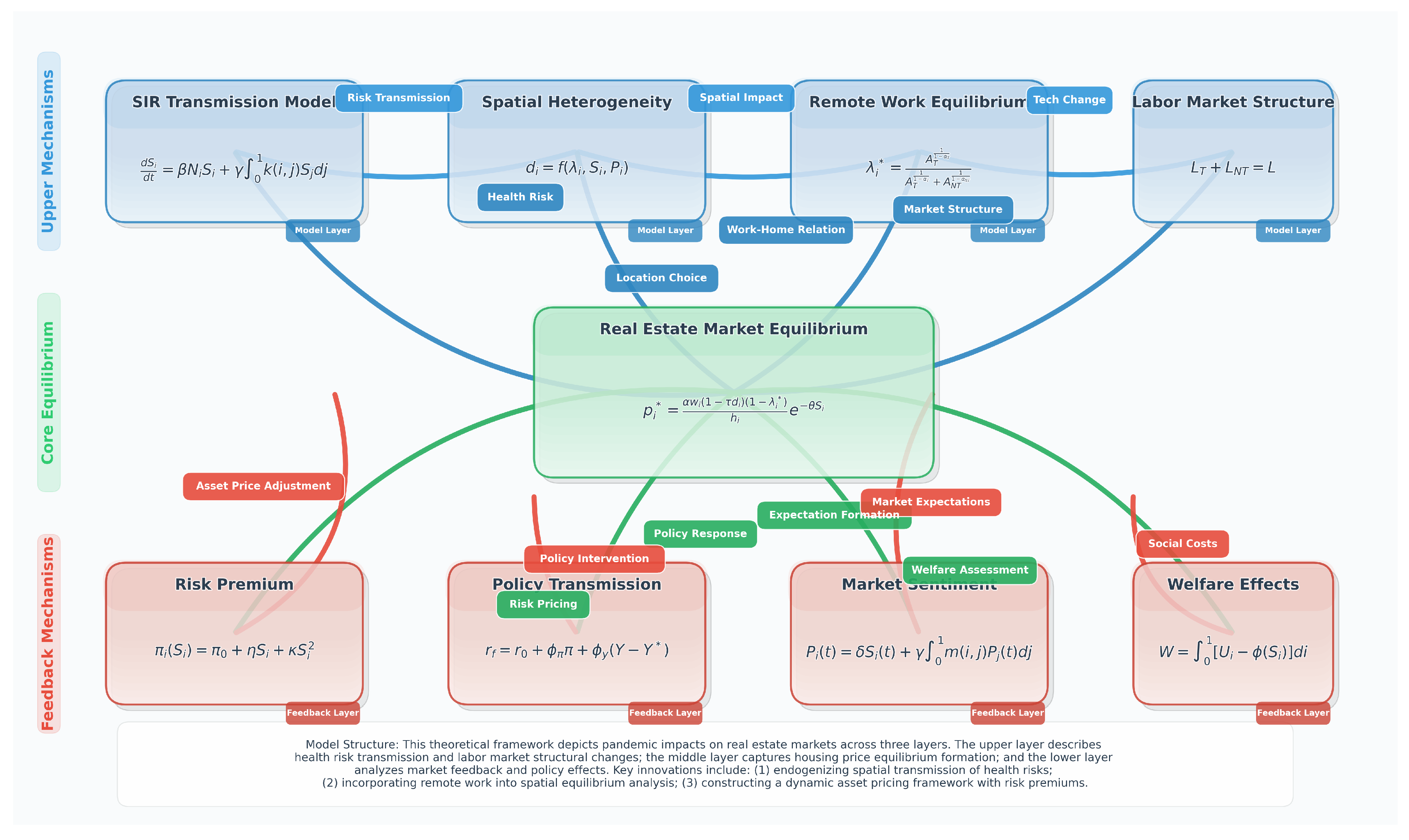

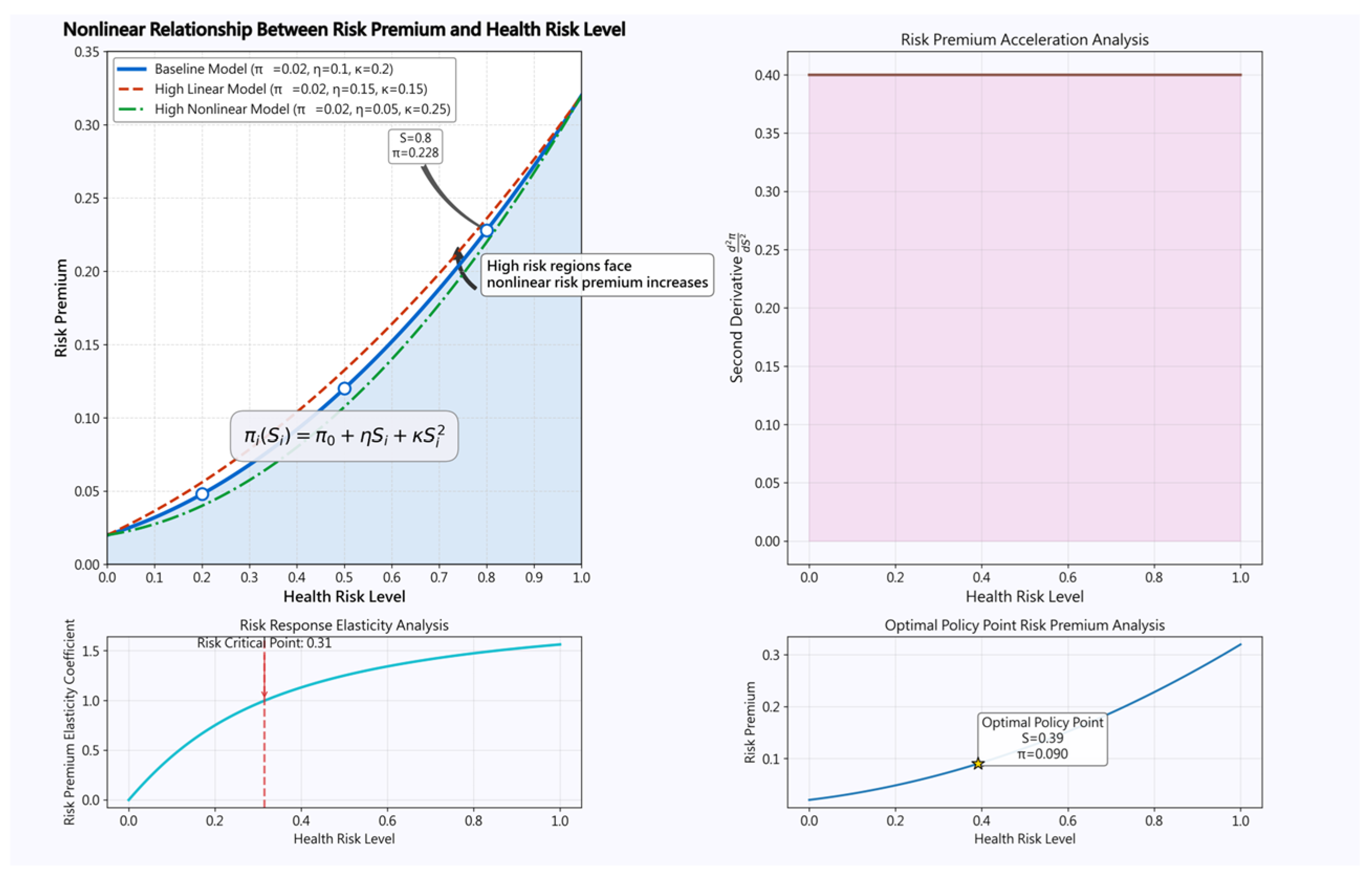

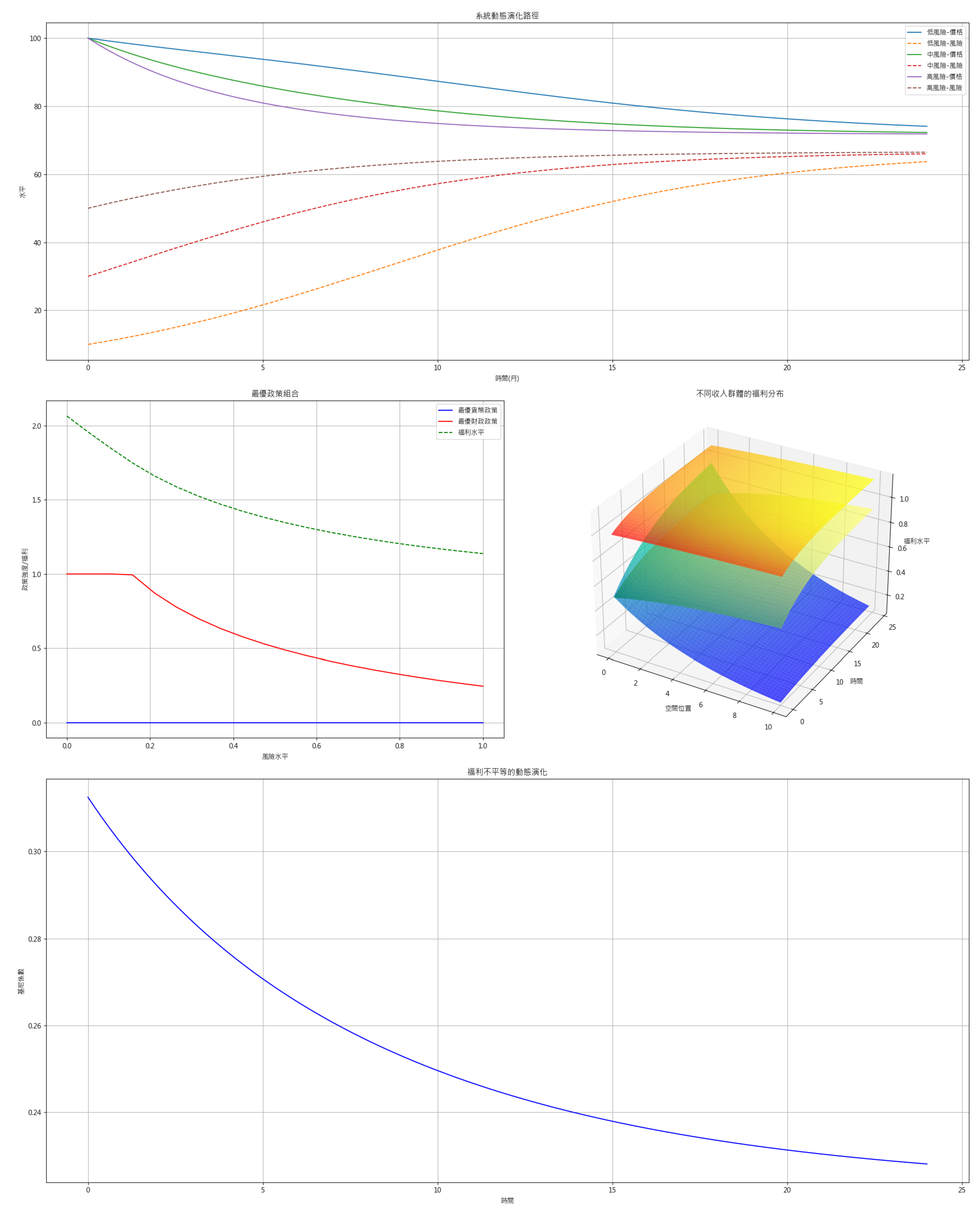
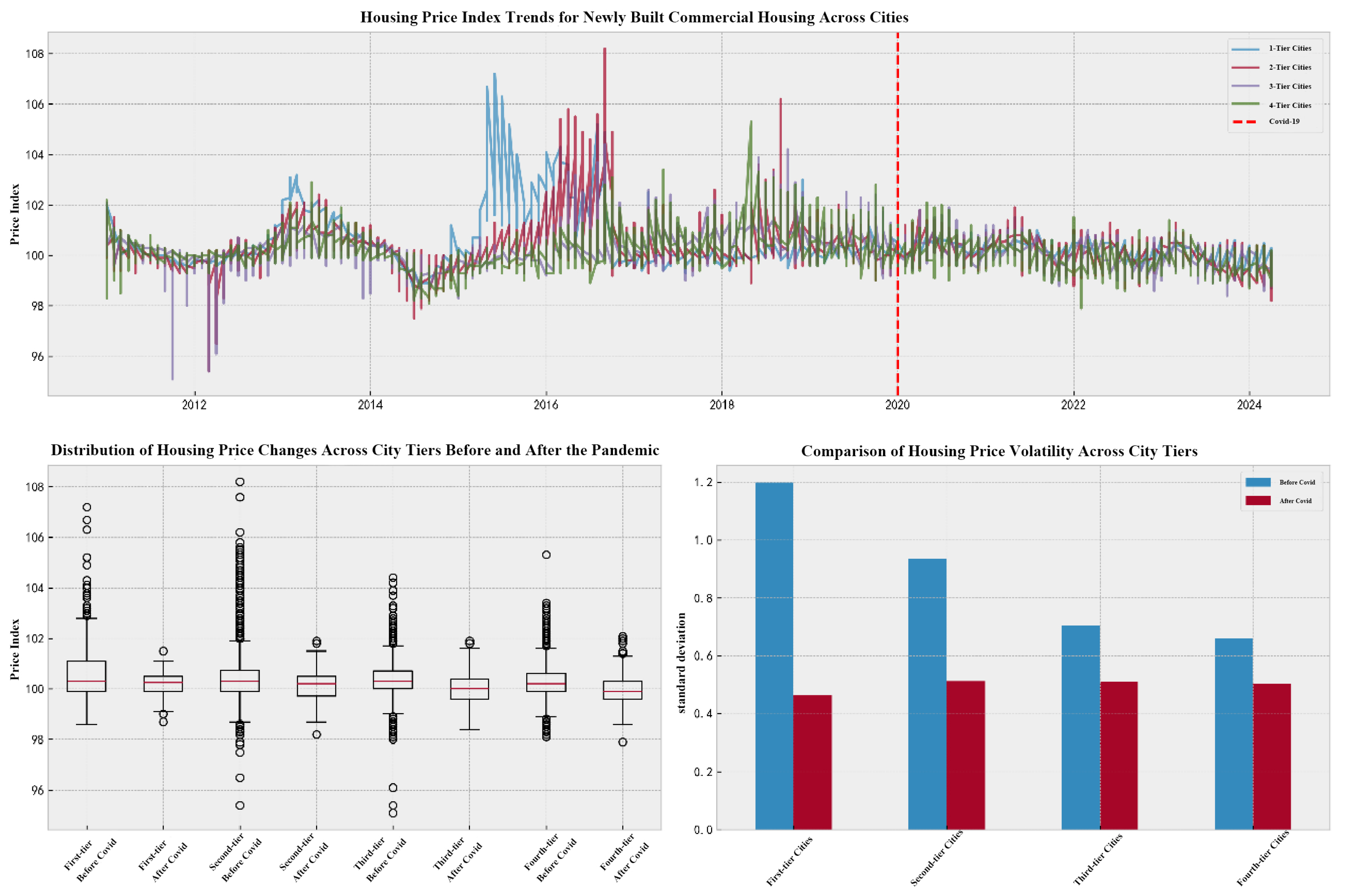
Disclaimer/Publisher’s Note: The statements, opinions and data contained in all publications are solely those of the individual author(s) and contributor(s) and not of MDPI and/or the editor(s). MDPI and/or the editor(s) disclaim responsibility for any injury to people or property resulting from any ideas, methods, instructions or products referred to in the content. |
© 2025 by the author. Licensee MDPI, Basel, Switzerland. This article is an open access article distributed under the terms and conditions of the Creative Commons Attribution (CC BY) license (https://creativecommons.org/licenses/by/4.0/).