Concrete Carbonization Prediction Method Based on Bagging and Boosting Fusion Framework

Abstract

Concrete carbonation is an important factor causing corrosion of steel reinforcement, which leads to damage to reinforced concrete structures. To address the problem of concrete carbonation depth prediction, this paper proposes a prediction model. The framework synergistically integrates Bagging and Boosting algorithms, specifically replacing the original Random Forest base learner with gradient Boosting variants (LightGBM (version 4.1.0), XGBoost (version 2.1.1), and CatBoost (version 1.2.5)). This hybrid approach exploits the strengths of all three algorithms to reduce variance and bias, and to further improve prediction accuracy, Bayesian optimization algorithms were used to fine-tune the hyperparameters, resulting in three hybrid-integrated models: Random Forest–LightGBM Fusion Framework, Random Forest–XGBoost Fusion Framework, and Random Forest–CatBoost Fusion Framework. These models were trained on a dataset containing 943 case sets and six input variables (FA, t, w/b, B, RH, and CO₂). The models were comprehensively evaluated using the comprehensive scoring formula and Taylor diagrams. The results showed that the hybrid-integrated model outperformed the single model, with the RF–CatBoost fusion framework having the highest test set performance (R² = 0.9674, MAE = 1.4199, RMSE = 2.0648, VAF = 96.78%). In addition, the Random Forest–CatBoost Fusion Framework identified exposure t and CO₂ concentration as the most important features. This paper demonstrates the applicability of a predictive model based on the Random Forest–CatBoost Fusion Framework in predicting the depth of concrete carbonation, providing valuable insights into the durability design of concrete.

1. Introduction

Concrete carbonation is the ingress of acidic carbon dioxide (CO₂) gas from the air through defects in the concrete surface (e.g., pores, cracks, etc.) and the carbonation reaction with alkaline substances in the concrete (Ca(OH)₂ and C-S-H gels, etc.) [1,2,3]. The process of producing the alkaline material is in decline, and the impact of carbonation on reinforced concrete is reflected in the neutralization of the concrete and the failure of the protective layer. The protective layer of the reinforcement will gradually deteriorate, leading to rusting under the combined effects of water and air, as well as other factors, while the corrosion products are caused by a two- to six-fold volume expansion. This, in turn, leads to concrete cracking, which accelerates the process of rusting. As a result, the concrete structure becomes detached from the protective layer, thereby reducing its bearing capacity. This, in turn, threatens the stability and safety of the structure.

There are many factors that affect carbonization behavior, including concrete’s service environment factors (temperature, relative humidity, CO₂ concentration, etc.) and its own quality factors (auxiliary cementitious material content, water–cement ratio, cement content, etc.).

Relative humidity (RH) is defined as the humidity condition in the service environment. It has been shown that environmental RH significantly affects the rate of concrete carbonation, as it influences the water content within the concrete’s pore structure. Wierig [4] found the fastest rate of carbonation to be in the range of 50–70 per cent RH, with a maximum point of approximately 55 per cent, through long-term observations. Papadakis et al. [1] found the fastest rate of carbonation to be in the range of 50–60 per cent RH, with a maximum point of about 55 per cent, through accelerated carbonation tests.

The effect of ambient temperature on the rate of carbonation is primarily evident in the effect of temperature on the rate of the carbonation reaction [5]. Papadakis et al. [1] conducted carbonation experiments within the temperature range of 22–42 °C at constant RH levels, and the results demonstrated that the effect of temperature variation on the rate of carbonation was limited and almost negligible. Bahador [5] utilised the Arrhenius formula to apply a temperature correction to the rate of carbonation.

$$x_c\left(T=298 \mathrm{K}\right)=x_c\left(T\right)·\mathrm{e}\mathrm{x}\mathrm{p}(8.6-{\displaystyle \frac{2563}{T}})$$

(1)

where $x_c$ is the depth of carbonization (mm), and T is the absolute ambient temperature (K). The correction is based on an absolute temperature of 298 K as the base temperature. The correction is made considering the impact of temperature on the reaction rate. When the ambient RH is high, and the carbonation process is primarily governed by CO₂ diffusion, temperature changes have a minimal effect on the overall carbonation rate.

The porosity of cementitious materials typically decreases after carbonation [6]. However, Ngala and Page [6] found that the chloride ion and oxygen diffusion coefficients of specimens before and after carbonation were significantly increased when tests were compared. This finding indicates that carbonation reduces the concrete’s ability to resist the diffusion of ions and gases, which adversely affects its durability. The most direct effect of carbonation on reinforced concrete structures in general environments is to decrease the alkalinity of the concrete pore solution near the reinforcing bars, leading to the deobturation of the reinforcement and inducing corrosion [7,8,9,10].

Cement type and content directly affect concrete’s carbonatable material [11]. As cement production accounts for 8–10% of global industrial CO₂ emissions [12], researchers use supplementary cementitious materials (SCM) like silica fume (SF), fly ash (FA), and limestone (LS) to reduce environmental impact while altering carbonation behavior. RILEM TC 281-CCC [13] reported SCM concrete carbonation rates under identical conditions as FA > SF > LS. Zhang et al. [14] compared the effect of different fly ash admixtures and water–cement ratios on the carbonation of fly ash concrete through carbonation tests under natural curing conditions. The findings suggest that increasing the fly ash admixture and water–binder ratio would somewhat weaken the resistance to carbonation. However, reducing the water–binder ratio can effectively mitigate the deterioration of concrete caused by the fly ash admixture. Cheng et al. [15] found that fly ash can accelerate the carbonation process of concrete, with the average carbonation rate increasing significantly as the fly ash dosage rises. They also demonstrated a positive correlation between the carbonation depth of concrete and the amount of fly ash used. A strong correlation has been identified between the water-to-cement ratio and the carbonation depth [16]. It has been shown that a higher water–cement (w/c) ratio leads to increased internal porosity in concrete, which in turn accelerates the diffusion rate of CO₂ and promotes a faster carbonation rate.

Numerous studies have been conducted to date on predicting the carbonation depth of concrete. Empirical formulas, regression analysis of experimental data, and finite element diffusion analysis have typically been utilized to establish a prediction model for concrete carbonation depth [17,18]. Fick’s diffusion law is one of the most frequently employed models for predicting the carbonation depth [19]:

$$x_c=k\sqrt{t}$$

(2)

where $x_c$ is the carbonation depth, k is the carbonation rate coefficient, and t is the carbonation time. The carbonation rate coefficient k is determined by the concentration of CO₂ in the exposed environment, the diffusion coefficient of CO₂ in the concrete, and the CO₂ absorption property of the concrete.

However, accurately developing a prediction model for concrete carbonation typically requires a large amount of data, leading to complex calculations and statistical challenges.

The advent of artificial intelligence (AI) has precipitated the emergence of machine learning (ML) methodologies, which have emerged as a novel solution for the resolution of intricate, non-linear engineering challenges [20]. ML algorithms are well suited for addressing complex, non-linear, multi-factor problems. With their robust data analysis capabilities, they can efficiently identify optimal solutions. They have been widely used in engineering research related to predictive analysis and optimization [21]. In recent years, machine learning algorithms such as Random Forest (RF) and artificial neural network (ANN) have seen widespread use in engineering fields [22]. For example, Londhe et al. [23] predicted the carbonation depth of concrete by RF and represented the output in the form of multiple trees. Kellouche et al. [24] developed an ANN prediction model, which was in strong agreement with the experimental data. P. Akpinar et al. [25] used an ANN and presented two models with different training learning schemes, and the results showed that the use of ANN to predict carbonation depth can provide satisfactory accuracy. Models such as XGBoost, LightGBM, and CatBoost have good prediction accuracy and efficiency compared to traditional machine learning algorithms [26]. For example, Kumar et al. [27] used three machine learning models (i.e., Adaboost, Random Forest, and XGBoost) to predict the permeability values of blended concrete containing Blast Furnace Slag (BFS) and FA. Both Adaboost and XGBoost showed excellent accuracy [27]. Wu et al. [28] combined GBDT with Particle Swarm Optimization Algorithm (PSO) and Sparrow Search Optimization Algorithm (SSA) to form two hybrid models, PSO-GBDT and SSA-GBDT, and compared them with the three classical models, namely, GBDT, ANN, and SVR, which showed that the two hybrid models show better prediction performance in the dataset.

However, individual ML models may be susceptible to overfitting and local minima issues, potentially resulting in an inadequate capture of the underlying data patterns present within the dataset [29]. In order to address this issue, some researchers have developed hybrid-integrated ML models that integrate multiple independent models for the purpose of achieving more accurate and efficient predictions [30,31]. For example, Wang et al. [32] proposed the Sand Cat Swarm algorithm (SCSO) to optimize the hyperparameters of three integrated models, leading to the creation of three hybrid models: SCSO-GBDT, SCSO-LGBM, and SCSO–CatBoost. All three models were effective in accurately predicting the carbonation depth of fly ash concrete, with the SCSO–CatBoost model demonstrating the best performance. Huo et al. [33] developed two integrated models based on the inverse variance method and artificial neural network, which are more accurate than single models in predicting the carbonation of concrete. Han et al. [34] applied an RF-SVM integrated machine learning model for the first time to predict the modulus of elasticity (MOE) of recycled aggregate concrete with high accuracy, which outperformed a single model.

Many existing prediction models require a pre-assigned and pre-determined selection of unexplained features, often derived from empirical experiments, and the incorporation of explainable features into the prediction model is critical to improving accuracy and practical applicability [35]. In recent years, research in the field of carbonation depth prediction has begun to incorporate interpretable characterization features in prediction models in order to address related issues. For example, Wang et al. [32] used various machine learning models as well as predictive equation models to predict the carbonation depth of recycled concrete. The prediction results were quantitatively analyzed and interpreted using SHAP value analysis. This method shows obvious advantages in explaining the carbonation factors of recycled concrete.

Bagging and Boosting are two commonly used integrated learning methods. Bagging involves constructing multiple Bootstrap training sets from a given dataset, and each base learner is trained on these sets to generate an ensemble of base learners [36]. In contrast, Boosting assigns weights to the training samples and modifies these weights dynamically according to the classifier’s performance on the training data. For misclassified samples, their weights are increased, thus enabling adaptive tuning of the training set distribution, and the performance of each classifier influences the training process of the next classifier [37].

Although previous studies have applied Bagging or Boosting methods to predict the carbonation depth of concrete, there is still room for improvement in the prediction accuracy of a single model. The integration of Boosting into the Bagging structure can simultaneously reduce the variance and bias, more accurately predict the carbonation depth of concrete, and systematically analyze the roles of various influencing factors. Therefore, in this study, an RF–CatBoost-based fusion framework (RCFF) [38] was developed to predict the carbonation depth of fly ash concrete. A dataset was compiled from the existing literature, including six specific input parameters and carbonation depth as the output variable, and the data were subjected to statistical analysis. A Bayesian optimization algorithm was employed to search for the optimal hyperparameters across seven different models, namely RF, LightGBM, XGBoost, CatBoost, RCFF, RLFF (a fusion framework based on RF– LightGBM), and RXFF (a fusion framework based on RF–XGBoost), and four performance evaluation methods were used for comparing the different model performance differences. Subsequently, SHAP was utilized on the optimal hybrid integration model for interpretability analysis, aiding in the understanding of the relationship between input features and carbonation depth. The model’s prediction results can serve as a valuable reference for enhancing concrete durability in engineering applications. It provides a data-driven theoretical basis for the durability design of concrete structures and the development of carbonation protection strategies. Compared with traditional empirical formulations or experimental methods, RCFF can effectively handle a large number of multidimensional input variables and their complex interactions, resulting in a more comprehensive assessment of the carbonation process.

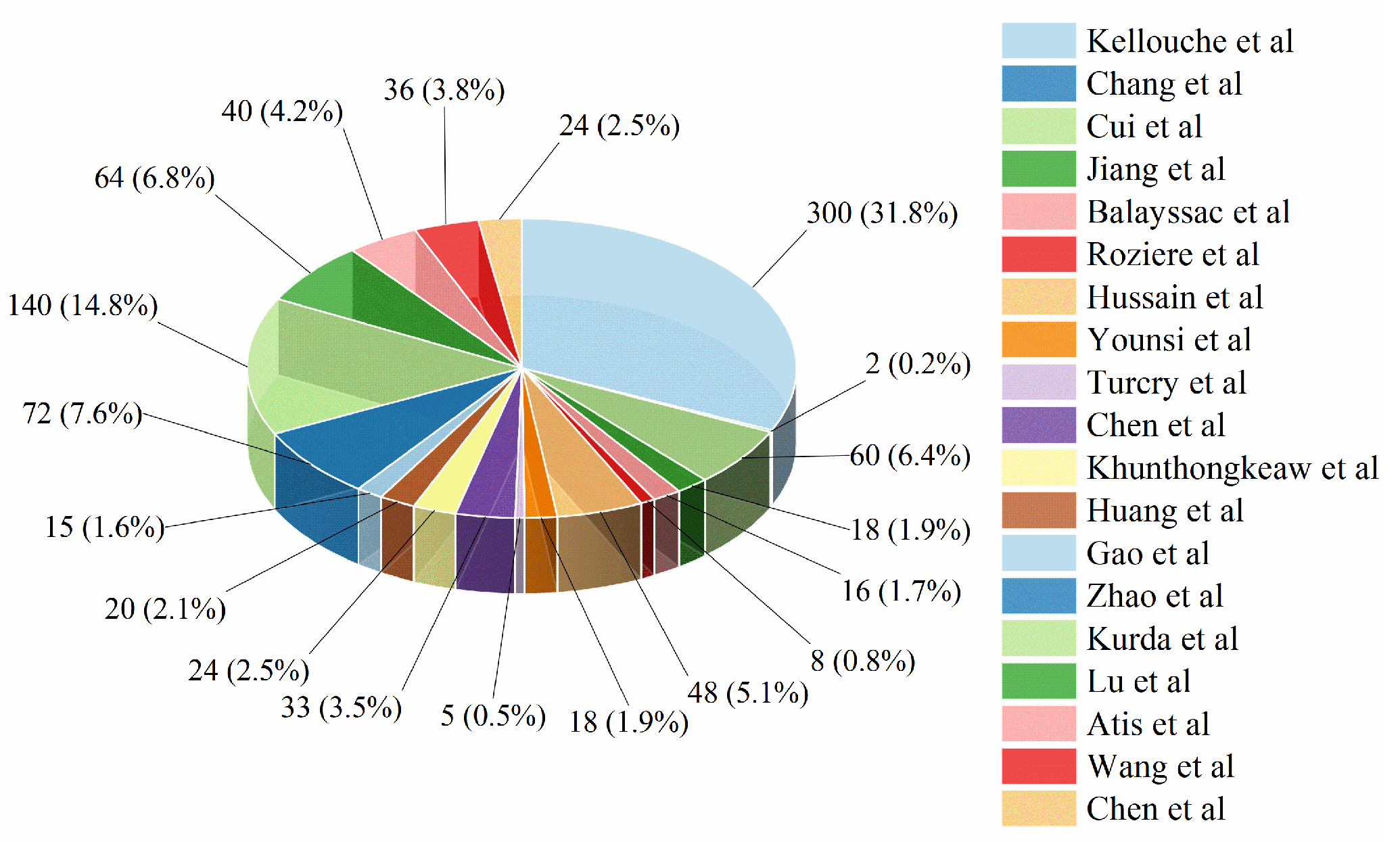
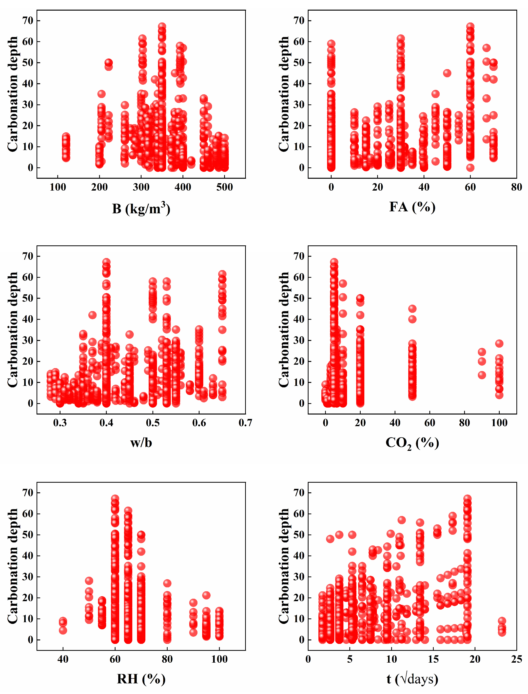
2. Dataset Description and Analysis

In this paper, RFCC is used to investigate the six main features affecting the depth of concrete carbonation, i.e., cement dosage (B), fly ash dosage (FA), water–cement ratio (w/b), relative humidity (RH), CO₂ concentration, and exposure time (t), which are used as input features to the model and the output is the depth of concrete carbonation (X). For this purpose, a database collected from the relevant literature [11,24,39,40,41,42,43,44,45,46,47,48,49,50,51,52,53,54] was created, totaling 943 samples of concrete carbonation depth. The source and distribution ratio of the data are shown in Figure 1 (Specific data can be viewed in Supplementary Materials).

In this study, the database was visualized to facilitate data analysis.

Table 1. Statistical descriptions of the variables in the dataset.

	Input						Output
	B (kg/m3)	FA (%)	w/b	CO2 (%)	RH (%)	$\mathit{t}\left(\sqrt{\mathit{d}\mathit{a}\mathit{y}\mathit{s}}\right)$	X (mm)
Count	943	943	943	943	943	943	943
Mean	360.94	22.65	0.46	14.35	66.66	6.71	12.62
STD	74.39	22.18	0.09	16.30	9.44	4.71	12.55
Min	120.00	0.00	0.28	0.03	40.00	1.73	0.00
25%	325.00	0.00	0.39	5.00	60.00	3.74	4.00
50%	350.00	20.00	0.45	6.5	65.00	5.29	9.00
75%	400.00	39.60	0.53	20.00	70.00	7.94	17.00
Max	500.00	70.00	0.65	100.00	100.00	23.24	67.20

presents the descriptive statistics for each feature, while Figure 2 displays scatterplots illustrating the relationships between each input variable and the output variable. These visualizations help in understanding the distribution of features in the dataset. For instance, in the plot depicting the relationship between exposure time and carbonation depth, it can be tentatively inferred that prolonged exposure results in an increased carbonation depth. Figure 3 depicts the Pearson correlation coefficient (PCC) for each input variable relative to the output variable, ranging from −1 to 1 [55]. The correlation between different input and output variables can be visualized by calculating the PCC. Positive values indicate a positive correlation between two variables, while negative values suggest a negative correlation. According to the results in Figure 3, there is a strong positive correlation between the depth of concrete carbonation and its exposure time in this 943 sample data with a value of 0.47, which is predictable and has been demonstrated in the commonly used Fick diffusion model [56]. The correlation between concrete carbonation depth and CO₂ concentration was weak, with a value of 0.02. However, CO₂ has been demonstrated to be a key factor affecting carbonation depth in previous studies. Upon analyzing the correlation between the input variables, it was observed that, aside from the significant correlation between B and w/b, the remaining input variables exhibited weak correlations. This weak correlation makes it challenging to consider multiple variables simultaneously when predicting concrete carbonation depth using methods like the Fick diffusion model, ultimately resulting in reduced accuracy in long-term predictions. Meanwhile, the correlation coefficient serves as a tool for examining the interdependence within the data. When the correlation coefficient between two variables exceeds 0.80, a strong correlation is present. This type of situation is commonly known as the “multicollinearity problem” [57]. As depicted in Figure 3, the absolute values of all correlation coefficients are below 0.5. Consequently, there is no “multicollinearity problem” among the variables.

3. Methods

3.1. Machine Learning Algorithms

3.1.1. Random Forest Regression

The Random Forest algorithm is an integrated learning algorithm, first proposed by Breiman in 2001 [58], derived from the decision tree (DT) algorithm. Single models, such as decision trees or linear regression, are vulnerable to data noise, which can result in overfitting or underfitting. To address the shortcomings of individual models, researchers have proposed integration techniques, such as “Bagging” and “Boosting”, to improve the model’s generalization capacity. RF integrates the Bagging technique into DT generation and introduces randomly selected sample features. RF is widely utilized in carbonation prediction tasks. It has high performance in dealing with high-dimensional data with low computational cost and high parallel computing capability [59]. The method involves building several decision trees and combining their predictions through averaging (for regression tasks) or majority voting (for classification tasks) to generate the final output. RF first samples the training data randomly using Bootstrap Sampling, which randomly and retrospectively draws n samples from the original dataset (the same number as the original dataset) to form a sub-dataset and then randomly selects n samples (the same number as the original dataset) in the sub-dataset to form a sub-dataset. For the formation of sub-datasets, on the sub-datasets, the decision tree is trained. In the process of generating, the decision tree will be formed because of the different sub-datasets and different structures, and finally, the final prediction is output by integrating the results of multiple decision trees.

3.1.2. Categorical Boosting (Catboost)

CatBoost (version 1.2.5) is a machine learning algorithm based on gradient Boosting, released by the Russian company Yandex in 2018 [60]. It has the unique advantage of efficiently processing categorical data. In the field of machine learning, CatBoost has superior generalization ability and model stability compared to other decision tree-based Boosting algorithms such as XGBoost (version 2.1.1) and LightGBM (version 4.1.0) [60,61]. Unlike traditional GBDT, CatBoost uses a symmetric tree structure, i.e., the same splitting decision is made simultaneously on multiple branches of each tree. This approach accelerates both the training and prediction processes of CatBoost while simultaneously improving the model’s generalization capability. For regression tasks, CatBoost optimizes an explicit objective function combining a loss function (e.g., mean squared error, $L(y,F)={\displaystyle \frac{1}{N}}\sum _{i=1}^N (y_i-F_i{)}^2)$ and regularization terms (e.g., L2 penalty on leaf weights). Moreover, CatBoost enhances the conventional GBDT gradient estimation by incorporating stochastic gradient descent (SGD), which helps mitigate the issue of gradient drift and boosts the model’s robustness. In the training process, CatBoost gradually generates new decision trees, each trained to approximate the negative gradient (pseudo-residuals) of the loss function with respect to the current model predictions. The iterative process usually contains hundreds of decision trees, with each iteration minimizing the objective function $L\left(y,F\right)+\lambda {\Sigma }_{t=1}^T{\Sigma }_{j=1}^{J_t}={ w}_{t,j}^2$ where λ controls the strength of L₂ regularization on leaf weights w_t,j. To avoid overfitting, CatBoost further constrains model complexity by limiting tree depth and adjusting the learning rate η during the additive updates $F_t\left(x\right)={ F}_{t-1}\left(x\right)+\eta ·h_{t }\left(x\right)$. Finally, the prediction results of all decision trees are integrated and averaged. This integrated output makes the model more stable with higher generalization ability.

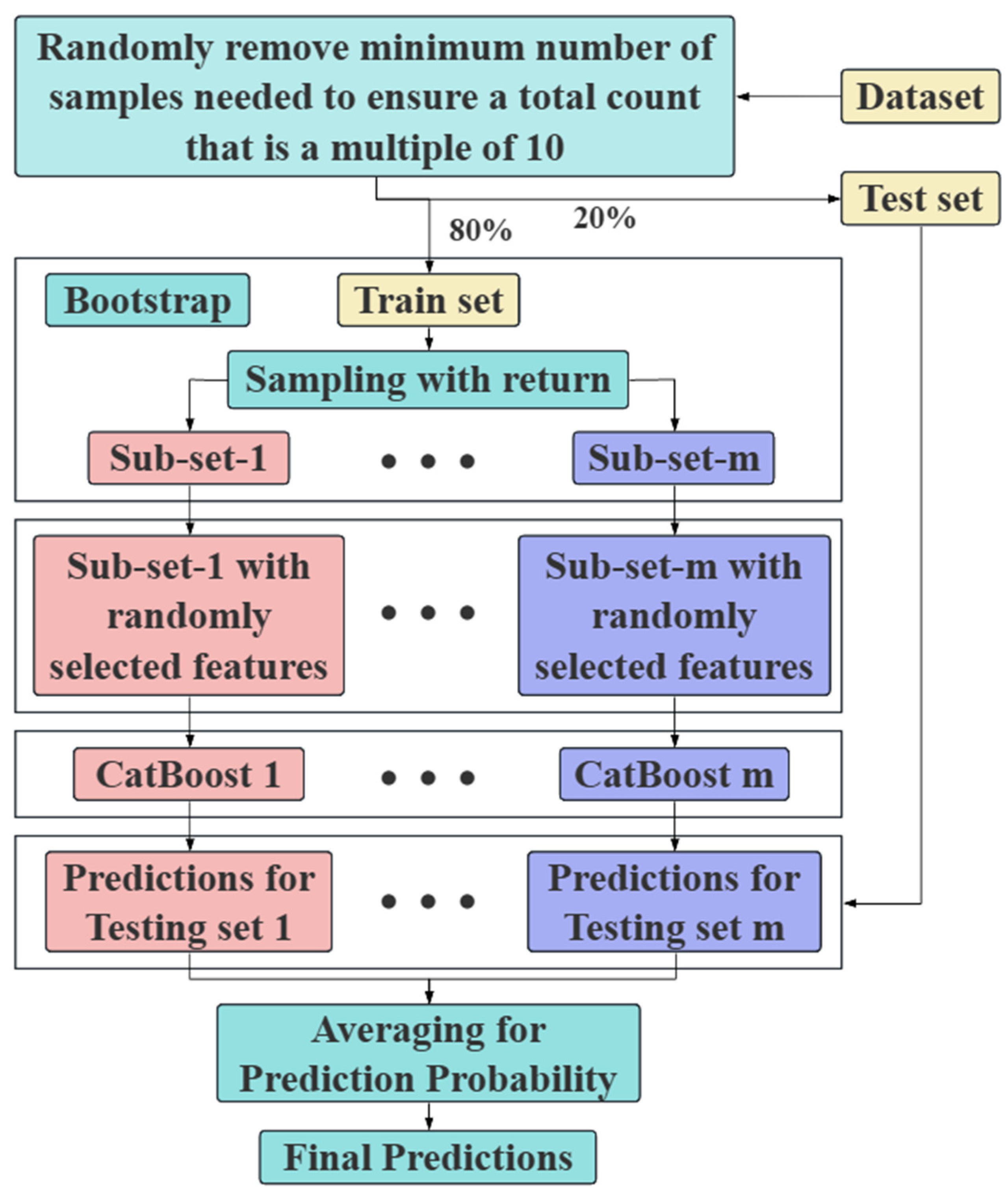
3.1.3. RF–CatBoost-Based Fusion Framework

Bagging methods are good at reducing the prediction variance while Boosting methods are good at reducing the prediction bias. In order to utilize their respective strengths, the fusion framework that combines Bagging and Boosting was chosen to integrate CatBoost into the RF framework to synergize the strengths of these algorithms [35,39]. RCFF is composed of a series of independent CatBoost models. During the training process, bootstrapping is employed to generate multiple subsets from the original training set, and then m CatBoost models are individually constructed. Each CatBoost model provides a prediction for each instance, and the final output is determined by averaging the predictions from all the individual CatBoost classifiers. The construction of RCFF follows three phases: partitioning the sub-training set, constructing the m CatBoost models, and aggregating the results to obtain the final prediction. The detailed process is summarized as follows [38]. Figure 4 shows the workflow diagram of RCFF.

Phase 1: Partitioning of sub-training sets

To mitigate the issue of potential correlations among multiple CatBoost models trained on the same complete training dataset $\Omega ={\left\{\left(x_k,y_k\right)\right\}}_{k=1}^n$ (with n instances), a Bootstrap method is used to create m uncorrelated training sets ${\Omega }_j={\left\{\left(x_k,y_k\right)\right\}}_{k=1 }^n$ (j = 1,2,…,m). The Bootstrap method involves forming a new training set and replacing the original set using uniform sampling [38]. Instances may recur in different training subsets ${\Omega }_j={\left\{\left(x_k,y_k\right)\right\}}_{k=1}^n$ (j = 1,2,…,m), where a fraction (1$-$1/e$)$ ($\approx$63.2%) of the unique instances are duplicated, and the rest are duplicated [62]. Segmentation of the sub-training set using the Bootstrap method reduces the variance without increasing the bias, thus improving the prediction performance.

Phase 2: Construction of m CatBoosts

Given the newly generated subset ${\Omega }_j={\left\{\left(x_k,y_k\right)\right\}}_{k=1}^n$ ( j= 1,2,…,m), where $x_k=(x_k^1,x_k^2,···,x_k^w)$ represents a random vector with w features and $y_k\in \left\{0,1\right\}$ is a binary variable, each $\left(x_k,y_k\right)$ pair follows an independent and identical distribution governed by an unknown distribution Ξ(⋅, ⋅). The objective of the learning process is to train a function $F:R^m\to R$ that minimizes the expected loss $L\left(F\right)=\mathrm{E}L\left(y,F\left(x\right)\right)$, where L(⋅, ⋅) denotes a smooth loss function and (x,y) represents a test sample drawn from the training subset ${\Omega }_j$.

During the iterative process, gradient Boosting is employed to generate a series of approximations of ${ F}^t:R^m\to R t=$1, 2,… in a greedy way. Specifically, $F^t$ can be estimated based on the $F^{t-1}$ additively, that is, ${ F}^t=F^{t-1}+\alpha h^t$. Here, $\alpha$ denotes a step size and $h^t:R^t\to R$ is a base classifier chosen from a set of functions H with the goal of minimizing the expected loss; that is,

$$h^t=\underset{h\in H}{\mathrm{argmin}}L\left(F^{t-1}+h\right)=\underset{h\in H}{\mathit{argmin}}\mathrm{E}L\left(F^{t-1}\left(x\right)+h\left(x\right)\right)$$

(3)

Equation (3) can be solved using the Newton method by applying a second-order approximation of $L\left(F^{t-1}+h\right) \mathrm{a}\mathrm{t} F^{t-1}$ or via a (negative) gradient step. The gradient step ${ h }^t$ is determined by using $h^t\left(x\right)$ approximates $g^t \left(x,y\right)$, where $g^t\left(x,y\right)={\displaystyle \frac{\partial L\left(y,F^{t-1}\left(x\right)\right)}{\partial F^{t-1}\left(x\right)}}$ [38]. Generally, the least-squares approximation is employed, and Equation (3) can be further expressed as

$$h^t={\underset{h\in H}{\mathit{argmin}}\mathrm{E}\left({-g}^t\left(x,y\right)-h\left(x\right)\right)}^2$$

(4)

CatBoost introduces two key advancements: the use of ordered target statistics for handling categorical features and the implementation of ordered Boosting to address gradient bias. In the case of ordered target statistics, CatBoost first performs a random permutation of all instances. Then, it calculates the average label value for instances with the same categorical value that precedes the given instance in the permutation, denoted as $y_{{\delta }_s}$. Given a permutation $\delta =({\delta }_1,{\delta }_2,{···\delta }_n$), the original p-th permutated observation with categorical feature q is replaced by ${ x}_{{\delta }_{p,}q}$, and the mathematical expression of $x_{{\delta }_{p,}q}$ is

$$x_{{\delta }_{p,}q}={\displaystyle \frac{{\sum }_{s=1}^{p-1}\left[x_{{\delta }_{s,}q}=x_{{\delta }_{p,}q}\right]y_{{\delta }_{s,}}+\xi P}{{\overline{z}}_{s=1}^{p_{-1}}\left[x_{{\delta }_{s,}q}=x_{{\delta }_{p,}q}\right]+\xi }}$$

(5)

where P and $\xi$ denote the prior value and weight associated with the prior value, respectively. The prior value helps reduce noise, particularly in low-frequency categories. To address the issue of gradient bias inherent in traditional Boosting methods, CatBoost introduces ordered Boosting for calculating leaf values during tree structure determination. Specifically, based on the random permutation $\delta =({\delta }_1,{\delta }_2,{···\delta }_n$), for the i-th instance in the permutation dataset $x_i$, the gradient of the previous instances of $x_i$ is computed using the gradients of all preceding instances, i.e., ($x_1$, $x_2$, ⋅⋅⋅$x_{i-1}$). The tree is then scored by M_i, which estimates the gradient for $x_i$. This approach allows CatBoost to effectively mitigate the overfitting problem commonly observed in other gradient Boosting algorithms.

Phase 3: Aggregating the final predictions

The final model is composed of multiple CatBoost models, each trained on a newly generated sub-training set ${\Omega }_j={\left\{\left(x_k,y_k\right)\right\}}_{k=1 }^n$(j = 1, 2,…, m). The final prediction is obtained by averaging the predictions from all m CatBoosts models.

3.2. Hyperparameter Tuning

In the hyperparameter tuning of RCFF, a Bayesian optimization algorithm (BOA) is used to obtain more efficient and accurate prediction results. BOA is an optimization method based on Bayesian inference. The core idea is to use a probabilistic model (usually a Gaussian process) to construct the prior distribution of the objective function [63]. The acquisition function is used to guide the selection of new hyperparameters, and the optimal value of the objective function is found by iteratively updating the prior distribution. Compared with grid search and random search, BOA reduces the number of unnecessary attempts through the cooperation of the probabilistic model and acquisition function, which makes hyperparameter tuning more efficient and accurate.

3.3. K-Fold Cross-Validation

The K-fold cross-validation technique is an effective method to prevent model overfitting. Many machine learning methods tend to exhibit poor generalization, demonstrating strong predictive performance during the training phase but struggling to maintain accuracy during testing. To address this situation, a 5-fold cross-validation (CV) method is used, where the data will be divided into 5 subsets during the hyperparameter optimization phase, and one subset will be selected as the validation set and the remaining 4 as the training set in each round. A suitable combination of hyperparameters can significantly improve the predictive ability of the model [64]. The R² value of the validation set is computed to evaluate and compare the performance variations, helping identify the optimal combination of hyperparameters.

3.4. Performance Evaluation Indicators

In this paper, four evaluation metrics [65] were used to assess the prediction performance of individual and fusion models for carbonation depth, namely, the Coefficient of Determination (R²), the Root Mean Square Error (RMSE), the mean Absolute Error (MAE), and the Variance Accounted For (VAF). The formulas for each metric are provided as follows: where n represents the total number of samples, $y_i^{*}$ denotes the predicted value, $y_i$ represents the true value, and $\overline{y_i}$ indicates the mean value.

$$R^2=1-{\displaystyle \frac{\sum _{i=1}^n{\left(y_i-y_i^{*}\right)}^2}{\sum _{i=1}^n{\left(y_i-\overline{y_i}\right)}^2}}$$

(6)

$$\mathrm{M}\mathrm{A}\mathrm{E}={\displaystyle \frac{1}{n}}\sum _{i=1}^n\left|y_j-y_i^{*}\right|$$

(7)

$$\mathrm{R}\mathrm{M}\mathrm{S}\mathrm{E}=\sqrt{{\displaystyle \frac{1}{n}}\sum _{i=1}^n{\left(y_i-y_i^{*}\right)}^2}$$

(8)

$$\mathrm{V}\mathrm{A}\mathrm{F}=\left(1-{\displaystyle \frac{\mathrm{var}\left(y_i-y_i^{*}\right)}{\mathrm{var}\left(y_i\right)}}\right)\times 100\%$$

(9)

In the evaluation metrics, a lower MAE and RMSE value indicates better model performance. Conversely, the closer the R² and VAF values are to 1, the more favorable the model’s performance.

3.5. Explanatory Analysis of the Best Model

3.5.1. Global Significance Analysis and Local Output Explanation

Using the SHAP method, the contribution of input features to the carbonation depth is calculated in the best ML model, thus revealing the impact of each feature on the ML model [66]. The interpretability of the machine learning process is enhanced by this method, which also leads to an increase in the credibility of the model [26]. The marginal contribution of each input feature in the optimal machine learning prediction model is determined through attribution analysis using SHAP theory, which combines Equations (10) and (11).

Based on the additive nature of SHAP, the contribution of each input feature is quantified by Equation (10) [67,68].

$$Shaply\left(X_j\right)={\sum }_{S\subseteq N\backslash \left\{j\right\}}{\displaystyle \frac{k!\left(p-k-1\right)!}{p!}}\left(f\left(S\cup \left\{j\right\})-f(S\right)\right)$$

(10)

where p represents the total number of features; $N\backslash \left\{j\right\}$ denotes the set of all possible feature combinations, excluding $X_j$; S is a subset of the features from $N\backslash \left\{j\right\}$; $f\left(S\right)$ refers to the model’s prediction using the feature subset S; and $f\left(S\cup \left\{j\right\}\right)$ indicates the model’s prediction when including feature $X_j$ in the subset S.

On the basis of the above, the prediction of a single sample can be further explained. For each feature of the current sample, the marginal contribution of the feature when added to the subset is calculated over all possible subsets of features, considering all possible combinations of subsets. The sum of the Shapley values for each feature is equal to the difference between the model prediction and the baseline value, thus explaining the contribution of each feature to the current prediction. As shown in Equation (11),

$$f\left(x\right)=E\left[f\left(x\right)\right]+\sum _{j=1}^n{Shaply(X}_j)$$

(11)

where $E\left[f\left(x\right)\right]$ represents the average of all predicted values, and ${Shaply(X}_j)$ denotes the marginal contribution of feature j to the prediction.

3.5.2. Feature Interaction Analysis

Global importance analysis and feature importance analysis explain the model learning process from two perspectives, respectively; however, existing studies rarely analyze the interactions between multiple features. There are usually complex interrelationships between individual input features and other features that are intuitively unknown [26]. Even when two or more features are independent, they can occasionally exhibit a synergistic effect on the output values, which may be either positive or negative. In this case, identifying potential interactions between features is crucial for interpreting the interactions of input features [69]. The SHAP interaction value matrix plot illustrates the influence of the interaction between two features on the prediction outcomes.

3.5.3. Characteristic Importance Analysis

Feature importance analysis identifies the most influential features of the model’s output. By understanding which features hold the greatest significance, it becomes easier to interpret the underlying patterns within the data. To determine the overall contribution of each feature to the model’s prediction results, the average of the absolute values of the SHAP values is used as the contribution value ($\left|SHAP\right|$) [70], a higher ($\left|SHAP\right|$) indicates that the feature contributes more to the prediction results, thus indicating its importance in the model [71].

4. Results and Discussion

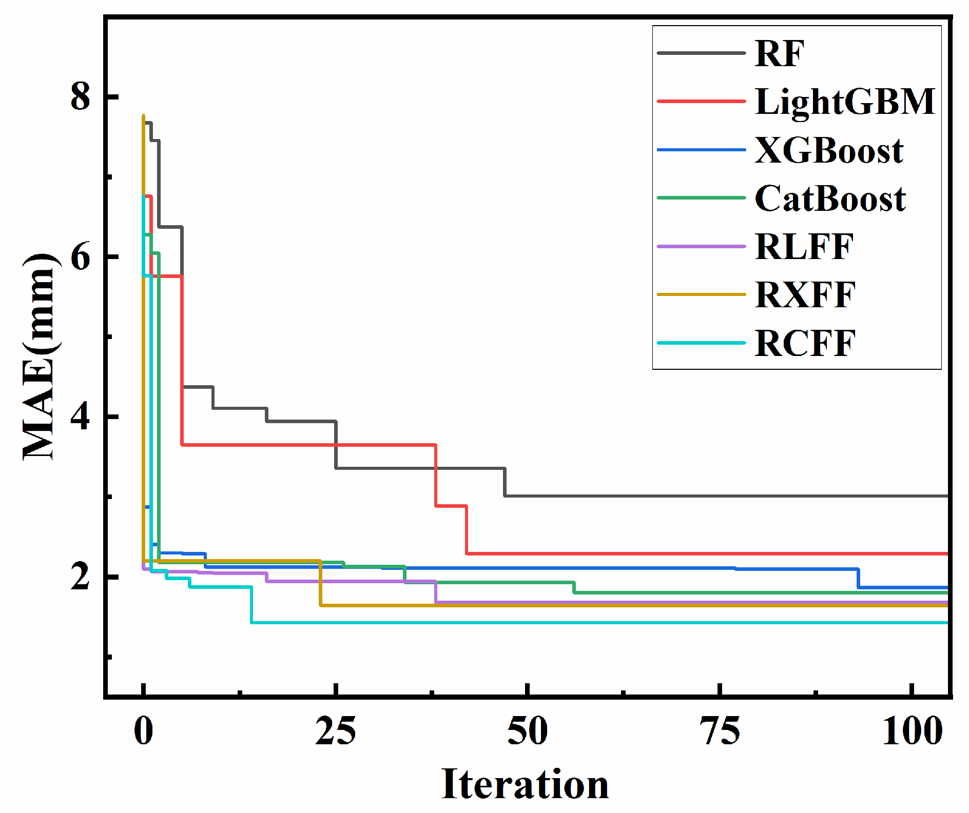
4.1. Hyperparameter Optimization

In this study, seven models were set up, including four individual models: RF, LightGBM, XGBoost, and CatBoost, and two fusion frameworks were constructed, based on RF–LightGBM (RLFF) and based on RF–XGBoost (RXFF), and the six models mentioned above were compared with RCFF, and the dataset was randomly split into a training set (80%) and a test set (20%) for model training. All models were optimized using a Bayesian algorithm for hyperparameters, and a five-fold cross-validation method was used to compare each model to verify the effectiveness of RCFF. The average R² was extracted from each iteration to find the optimal hyperparameter combination while going through 100 iterations by five-fold cross-validation and BOA methods.

Table 2. Candidate parameter setting of all models.

Model	Parameter	Scope	Optimal Value	Ave R2	MAE
RF	n_estimators	[50, 500]	282	0.8582	2.8687
	max_depth	[3, 10]	9
	min_samples_leaf	[1, 20]	1
	min_samples_split	[5, 20]	5
LightGBM	n_estimators	[50, 500]	398	0.9401	2.0865
	learning_rate	[0.01, 1]	0.31
	max_depth	[3, 10]	4
	num_leaves	[20, 100]	48
	min_child_samples	[5, 30]	18
XGBoost	n_estimators	[50, 500]	487	0.9432	1.8069
	learning_rate	[0.01, 1]	0.50
	max_depth	[3, 10]	3
	reg_lambda	[1, 10]	3
CatBoost	iterations	[50, 500]	427	0.9455	1.7018
	learning_rate	[0.01, 1]	0.39
	max_depth	[3, 10]	4
	l2_leaf_reg	[1, 10]	2
RLFF	Number of DTs inLightGBMs	[50, 500]	234	0.9483	1.5243
	Nodes number of DTs in LightGBMs	[20, 100]	20
	Learning rate in LightGBMs	[0.01, 1]	0.20
	Maximum depth in LightGBMs	[3, 10]	4
	Minimum value of the sum of sample weights in each node of DTs in LightGBMs	[5, 30]	20
RXFF	Number of DTs in XGBoosts	[50, 500]	195	0.9501	1.5025
	Learning rate in XGBoosts	[0.01, 1]	0.21
	Maximum depth of DTs in XGBoosts	[3, 10]	4
	Minimum number of samples contained in the nodes of DTs in XGBoost	[1, 20]	9
RCFF	Number of DTs in CatBoosts	[50, 500]	483	0.9524	1.4262
	Learning rate in CatBoosts	[0.01, 1]	0.23
	Depth of DTs in CatBoosts	[3, 10]	4
	Minimum number of samples contained in the nodes of DTs in CatBoosts	[1, 20]	12

shows the range of hyperparameter optimization, the optimization results, and the average R² for each model. In this study, the approximate range of hyperparameters for each model is determined through repeated trial and error, and a sufficient range of optimization is selected for each model to ensure optimal results and the fairness of the comparisons. Figure 5 depicts the model’s iterative process to find the optimal hyperparameter combination by calculating the average MAE value of the model on the validation set through cross-validation. In the figure, RCFF reaches the lowest MAE value the fastest. In addition, the models using the fusion framework have improved speed and accuracy compared to the corresponding individual models, reflecting the effectiveness of the framework. It can be seen that RCFF has the highest average R²: 0.9524, followed by RXFF, RLFF, CatBoost, XGBoost, LightGBM, and RF (version 1.0.2), where the models of all three fusion frameworks have an improved performance compared to the individual models. Here, the number of single models generated in each of the three fusion models is taken as optimal as well as minimum number: 50 as tested by trial and error method.

4.2. Model Prediction Results

Building upon the previous study, all individual models and the fusion framework model were trained and tested using the optimal parameters. This led to a quantitative depiction of the relationship between the predicted carbonation depths from each model and the experimental data across the entire dataset. As shown in Figure 6 and Figure 7, the figures clearly highlight the discrepancies between the actual carbonation depth measurements and the model predictions. At the top of each sub-figure, the corresponding prediction model and the assigned random partition are displayed, with the specific evaluation index value shown in the upper left corner. The results indicate that all models, except for RF, demonstrate high prediction accuracy. By examining the performance of the seven models on both the training and test sets, it is evident that the fusion model outperforms the individual models. This is demonstrated by a reduced number of points falling outside the lines y = 1.2x and y = 0.8x, with a greater concentration of points along the y = x line. This is in line with the proposed framework that combines the advantages of Bagging and Boosting, making RCFF, RXFF, and RLFF have lower errors compared to RF, CatBoost, XGBoost, and LightGBM.

The values of the four statistical error metrics for the seven models on the training and test sets are provided in

Table 3. Performance evaluation of different models with statistical error indicators.

	Model	R2	MAE	RMSE	VAF	Si
Training	RF	0.9453	2.0026	2.8428	94.53%	0.8930
	LightGBM	0.9852	0.8515	1.4449	98.52%	0.9554
	XGBoost	0.9865	0.7849	1.3808	98.65%	0.9583
	CatBoost	0.9871	0.7982	1.3831	98.71%	0.9583
	RLFF	0.9877	0.6908	1.3209	98.77%	0.9616
	RXFF	0.9881	0.7096	1.3269	98.81%	0.9614
	RCFF	0.9884	0.6727	1.3112	98.84%	0.9625
Testing	RF	0.8960	2.6786	3.6869	89.62%	0.8432
	LightGBM	0.9507	1.9493	2.7754	95.07%	0.8977
	XGBoost	0.9583	1.7256	2.5506	95.83%	0.9091
	CatBoost	0.9607	1.6105	2.2666	96.09%	0.9166
	RLFF	0.9617	1.4958	2.2362	96.18%	0.9198
	RXFF	0.9623	1.4826	2.2205	96.23%	0.9205
	RCFF	0.9674	1.4199	2.0648	96.78%	0.9267

, which further supports that the fusion models have higher predictive power than the individual models. RF performs relatively weakly in all the metrics.

Its test set R² is only 0.8960, and its MAE and RMSE values are higher (2.6786 and 3.6869, respectively) compared to other models based on Boosting techniques, indicating that its prediction error is relatively large. The VAF of RF is 89.62%, which also indicates that its ability to explain the data variance is limited. The results of LightGBM and XGBoost, as Boosting models, perform significantly better than RF, with their test set R² reaching 0.9507 and 0.9583, MAE and RMSE 1.9493, 2.7754 and 1.7256, 2.5506, respectively, and their VAFs also reaching 95.07% and 95.83%. Nevertheless, the error metrics of LightGBM and XGBoost are slightly inferior to those of the CatBoost model. RCFF, RXFF, and RLFF have better prediction performances compared to their counterparts, with individual Boosting techniques showing improvements in performance on both the training and test sets. On the test set, R² is improved by 0.074, 0.040, and 0.117, respectively; MAE is reduced by 0.1906, 0.2430, and 0.4535, respectively; and RMSE is reduced by 0.2018, 0.3301, and 0.5392, respectively. The RLFF fetches the highest combined Boosting effect, while the RCFF has the lowest combined Boosting effect due to the fact that the CatBoost single model itself already has a high level of prediction accuracy, while the prediction accuracy of LightGBM for carbonation depth is lower in comparison, and it also precisely illustrates that the fusion framework of Bagging and Boosting has an excellent bias correction effect and anti-variance property for lower accuracy models, which makes the model’s ability to explain the variation of the output enhanced, and its ability of carbonation depth fitting ability is enhanced.

Comparing the magnitude of individual evaluation metrics alone is one-sided, and in order to comprehensively evaluate the effectiveness of each model in predicting the depth of carbonation, a composite scoring method was used in this study, which can combine multiple metrics to quantify the predictive performance of the models [72]. The following equation shows the comprehensive scoring formula, which is derived from the idea of multi-criteria decision analysis (MCDM) [73], which is based on the comparison of the distances between positive and negative ideal solutions, and calculates the comprehensive score using normalization and weighting [74].

$$S_i={\omega }_1·Norm\left(R_i^2\right)+{\omega }_2·\left[1-Norm\left(MA{E}_i\right)\right]+{\omega }_3·\left[1-Norm\left(RMS{E}_i\right)\right]+{\omega }_4·Norm\left(VAF\right)$$

(12)

where $Norm\left(·\right)$ denotes the normalization operation to scale the indicator values to between 0 and 1, ${\omega }_1,{ \omega }_2{, \omega }_3, {\omega }_4$ are the weights of each indicator, which satisfy ${\omega }_1 + {\omega }_2 + {\omega }_3 + {\omega }_4 = 1$. The setting of weights should be based on the demand of the problem. If the explanatory ability of the model is more important, the weights of R² and VAF can be increased (e.g., ${\omega }_1=0.3$, ${\omega }_4=0.3$). If the absolute error of the model is more important, the weights of MAE and RMSE can be increased (e.g., ${\omega }_2{ =0.3, \omega }_3=0.3$). Here, the default equilibrium weights are used (${\omega }_1 = 0.25$, ${\omega }_2{ = 0.25, \omega }_3 = 0.25, {\omega }_4 = 0.25$).

S_i in Table 3 is the comprehensive evaluation score of each model, and it can be intuitively seen that RCFF achieved the highest comprehensive evaluation score, highlighting its balanced overall performance in the carbonation depth prediction task, with high fitting accuracy, low error, and good variance interpretation.

Figure 8 presents a Taylor diagram that compares the performance metrics of the seven models. The diagram illustrates the R², standard deviation, and root mean square deviation (RMSD) of the models based on their performance on the test set. The further the radial direction from the center of the circle in the graph represents, the larger its standard deviation; the red dotted line is the standard deviation calculated based on the collected carbonation depth dataset, and the closer it is to the red dotted line, the closer it represents the standard deviation of the model prediction result to the result of the dataset; the direction of the circle is the magnitude of the correlation coefficient, which is gradually increasing clockwise from 0 to 1; the green rounded dotted line represents the magnitude of the RMSD, and the red five-pointed star point is the reference point. It can be seen that RCFF is the closest to the reference point, which represents that it has the highest R² and, at the same time, has a lower RMSD, indicating that it has the most superior prediction performance among the seven models. This figure effectively demonstrates the superiority of the hybrid integration model developed in this study.

4.3. SHAP Interpretation Analysis of the Best Model

4.3.1. Global Significance Analysis

Figure 9 illustrates the outcomes of the global importance analysis for the input features in the RCFF model. The figure uses varying colors to represent the different feature values; data points that are more red indicate higher feature values, whereas those with a bluer tone reflect smaller values. Additionally, as the value increases along the horizontal axis, the feature’s influence on the predicted results becomes more significant. The graph reveals that t has the most significant impact on the carbonation depth of concrete, followed by FA, B, CO₂ concentration, w/b, and RH in that order. Higher values of t and CO₂ concentration generally lead to an increased carbonation depth. The features FA and w/b exhibit a more complex, bidirectional influence, with both high and low values affecting the carbonation depth in non-linear ways. B also shows a mixed effect, but a higher total binder content tends to reduce carbonation depth. Exposure time demonstrates a clear positive correlation with carbonation depth, making it a crucial predictor in the model. However, other features, while also important, have more complex and non-linear effects, making their influence less direct. Despite this complexity, the SHAP interpretation emphasizes that this does not diminish their importance but rather underscores the intricate interactions between these features and carbonation depth. Figure 10 shows the impact of specific cases on the predicted results through visualization. The $E\left[f\left(x\right)\right]$ is 12.27 mm, which represents the average of all predicted values. It can be seen that the four parameters, t, FA, RH, and B, contribute negatively to the carbonation depth, with corresponding SHAP values of −5.3, −2.82, −1.38, and −0.51, whereas w/b and CO₂ contribute to the carbonation depth, with SHAP values of +0.35 and +0.1, respectively.

4.3.2. Analysis Results of Feature Interaction

Figure 11 illustrates the impact of feature interactions on the predicted values. The color shading of the dots in the figure reflects the magnitude of the respective feature values, while the horizontal axis represents the SHAP interaction values. Positive interaction values indicate a positive contribution to the predicted value from that combination of features, while negative values signify a negative contribution. The dot plots along the diagonal show the main effect of each feature, representing the individual contribution of each feature to the predicted value. The off-diagonal portion represents the interaction between two features. An interaction point distribution of two features that is more spread out and away from the zero value indicates that the two features synergize significantly in the sample, e.g., t shows a strong interaction effect with FA and CO₂, FA shows some interaction effect with w/b and RH, CO₂ shows a strong interaction effect with w/b, B has only a slightly strong interaction with w/b, and RH shows a weak interaction effect with all other features. A strong interaction effect represents a synergistic influence between the two features on the model’s prediction of carbonation depth, e.g., at longer times, CO₂ concentration may have an increased effect on carbonation depth. When the interaction effect is weak, it represents that the two features act almost independently of each other, e.g., the interaction values of RH and w/b have a narrow distribution and are concentrated around the zero value, indicating that the water–glue ratio and relative humidity act independently of each other in the model.

4.3.3. Analysis Results of Characteristic Importance

Figure 12 presents the outcomes of the feature importance analysis for the input features in the RCFF model. The average SHAP value for each feature, depicted in the figure, quantifies the overall effect of the feature on the prediction outcomes. The features are arranged in descending order of importance, with those ranked higher having a greater influence on the model’s predictions. In the figure, the average SHAP value for exposure time t is the largest (5.43), and the model is highly dependent on the exposure time, which is consistent with the fact that the carbonation depth usually has a square root growth relationship with increasing exposure time according to Equation (2) [19]. The SHAP average of CO₂ concentration was 3.81, which was ranked second. Under consistent conditions, a higher CO₂ concentration accelerates the surface carbonation reaction of concrete, resulting in a more pronounced increase in carbonation depth. The model identifies a significant effect of CO₂ concentration on the carbonation depth, which is consistent with the results of existing experiments [75]. The average SHAP value of FA is 3.56, which is ranked third. Fly ash, as a mineral admixture in concrete, alters both the pore structure and the chemical composition of the material, thereby influencing the rate of carbonation. As shown in the global importance analysis in Figure 9, a moderate amount of fly ash admixture enhances the pore structure of concrete, facilitating the advancement of the carbonation interface into the interior. The SHAP mean value for B was 2.78, ranking fourth. The total amount of cementitious materials influences the strength and density of concrete. A higher total binder content leads to a more compact matrix structure, especially under an optimal water–cement ratio (as indicated by the significant interaction in Figure 11) and favorable curing conditions. This typically reduces porosity and CO₂ diffusion rate, ultimately affecting the carbonation depth. The matching results are also shown in Figure 9, where the darker colored dots mostly correspond to SHAP values below zero. The mean SHAP value of 1.78 for w/b is of relatively low importance. Higher water–cement ratio concrete is more conducive to gas diffusion and water migration due to its higher initial porosity, and CO₂ will reach deeper in this porous structure more easily, resulting in carbonation that tends to progress inwards. w/b shows a strong interaction effect with CO₂ in the SHAP interaction analysis in Figure 11, which suggests that the model’s identification of the significance of the water–cement ratio is consistent with the carbonation mechanism. Although the effect of the water–ash ratio is not as significant as exposure time and CO₂ concentration, it is still a more important factor affecting carbonation. The mean SHAP value of relative humidity was 1.62, which had the smallest effect among all variables. The impact of relative humidity on the carbonation process is more intricate and non-linear, with its influence varying under different conditions. It has been shown that the maximum rate of carbonation occurs when the humidity is in the range of 50–70%. Too low humidity inhibits the carbonation chemistry, while too high humidity hinders the diffusion of CO₂ [4]. The SHAP value analysis highlighted the contributions of key features in predicting concrete carbonation depth, with exposure time and CO₂ concentration emerging as the most influential predictors. In contrast, relative humidity had the least impact. This analysis offers a scientific foundation for understanding the relative significance of each feature in the carbonation process.

4.4. Significance and Limitations of the Study

This study employed RCFF to accurately predict the depth of concrete carbonation and systematically analyze the role of various influencing factors. The aim was to provide a data-driven theoretical foundation for the durability design of concrete structures and the development of carbonation protection strategies. Compared to traditional empirical formulations or experimental methods, RCFF can effectively handle a large number of multidimensional input variables and their complex interactions, offering a more thorough evaluation of the carbonation process. In this study, the SHAP values were used to quantify the contribution of each input variable in the model, making the prediction results highly interpretable. This analysis highlights the dominant effects of exposure time, CO₂ concentration, fly ash content, and other factors on the carbonation process, providing a quantitative basis for optimizing concrete material design and protective measures. Additionally, this study presents a novel and effective numerical method for evaluating concrete durability, enabling the prediction of carbonation depth during the design phase. This approach aids in the scientific formulation of protective measures to mitigate the risk of structural deterioration throughout the service life of the structure, thereby reducing maintenance costs. This data-driven prediction framework not only enhances the accuracy of model predictions but also deepens the quantitative understanding of the sensitivity of various design parameters. It holds significant value for engineering practice and offers substantial potential for theoretical advancement.

Despite the promising results achieved in this study regarding the prediction of concrete carbonation depth, there are still notable limitations. Firstly, the model’s validity is highly dependent on the size and quality of the dataset used. The dataset in this study may be limited by insufficient sample size and uneven data distribution, which could hinder the generalization ability and prediction performance of the model. Consequently, future research should focus on expanding the dataset to ensure greater diversity and representativeness, thereby improving the applicability and robustness of the model across a broader range of scenarios. Second, although SHAP values provide an intuitive means for model interpretation, their results are also affected by the distribution of data features, multicollinearity among features, and model complexity. In the case of highly correlated features, SHAP values may not be able to fully isolate the independent effects of each feature, thus affecting the rigor of the interpretation. Additionally, the machine learning model in this study primarily relies on a data-driven approach to capture the complex non-linear relationships in the carbonation process without fully incorporating the physical mechanisms underlying carbonation. Therefore, future work could explore the integration of a physical model with the data-driven model to create a hybrid framework that combines the physical insights with the advantages of data-driven techniques. This approach could enhance the scientific accuracy and rationality of the prediction results.

In conclusion, this study presents a machine learning method with promising potential for predicting concrete carbonation depth. However, there is still room for improvement in terms of the model’s generalization ability, data quality, and integration with the physical mechanisms of carbonation. These limitations highlight clear directions for future research, including optimizing the carbonation prediction model and enhancing the reliability and credibility of the prediction results.

5. Conclusions

In this paper, a concrete carbonation dataset containing 943 samples was established. The dataset was statistically analyzed and evaluated for relevance. The amount of cementitious material, fly ash admixture, water–cement ratio, CO₂ concentration, relative humidity, and exposure time were selected as the input variables, and the depth of carbonation as the output variable, and the modeling was carried out by using the RCFF framework. The RCFF, by combining the techniques of Bagging and Boosting, the CatBoost algorithm was utilized to capture the complex non-linear relationships and adjust the hyperparameters through Bayesian optimization. In addition, the model performance is assessed by the metrics of R², RMSE, MAE, and VAF and combined with SHAP analysis to reveal the contribution and interaction of input features. The main research conclusions are as follows:

(1)

The RCFF model outperforms single models (RF, CatBoost, LightGBM, XGBoost) and other fusion models (RLFF, RXFF) on both the training and test sets. The R² of the test set reaches 0.9674, the MAE is 1.4199, the RMSE is 2.0648, and the VAF is 96.78%, which is significantly better than the rest of the models, indicating that RCFF effectively improves the prediction accuracy through the advantages of the fusion framework;

(2)

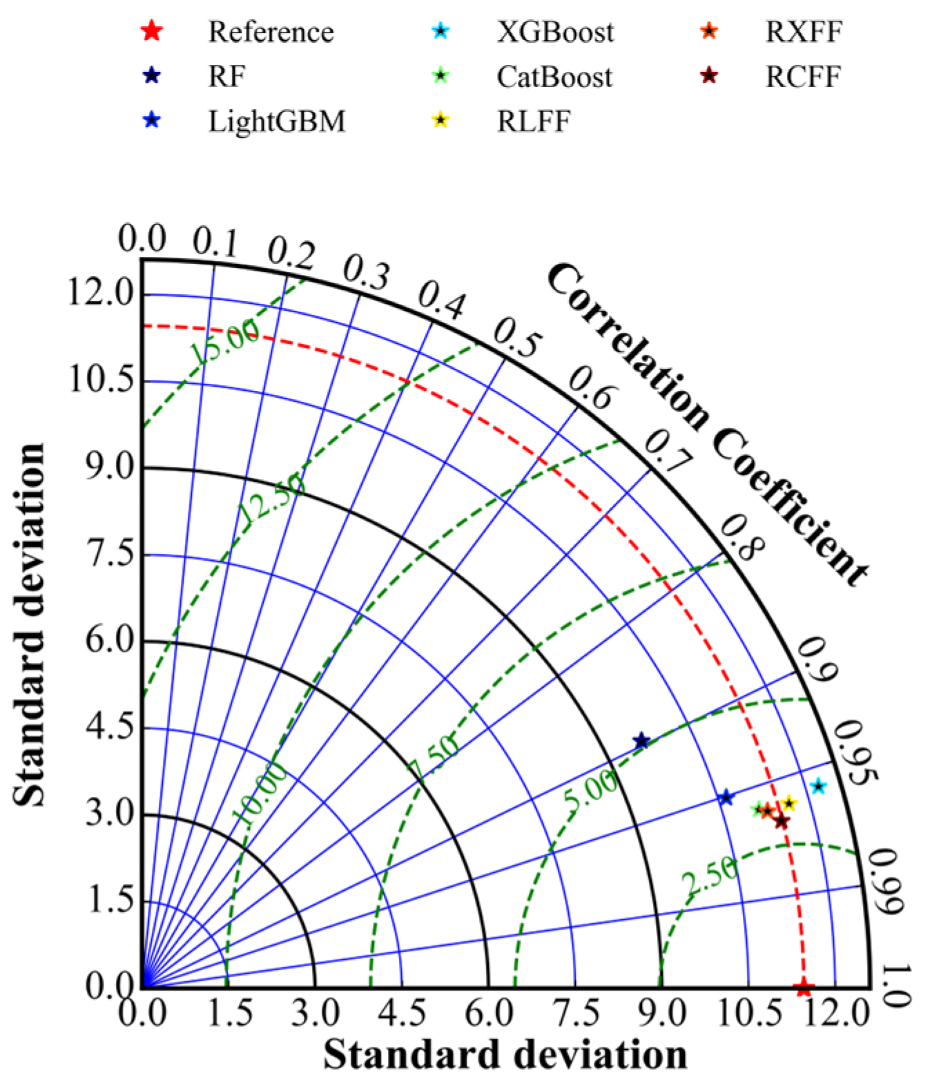
The prediction ability of each model on the test set was comprehensively evaluated and compared through the comprehensive scoring formula as well as Taylor diagrams. The results of the study show that RCFF has the highest comprehensive score. Taylor diagrams further visualize the performance of multiple performance metrics of different models, corroborating the excellent performance of the hybrid integration framework proposed in this paper in carbonation depth prediction;

(3)

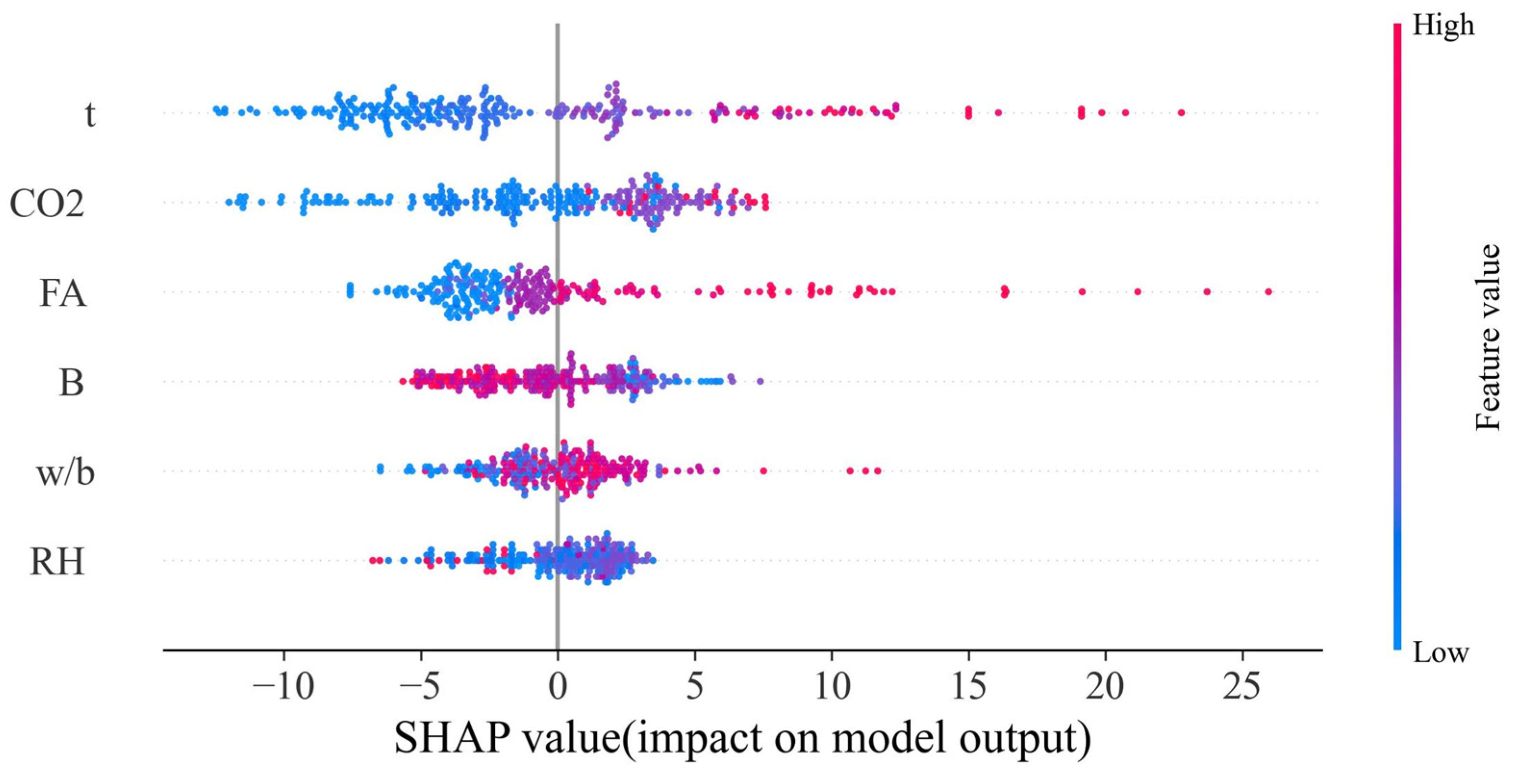
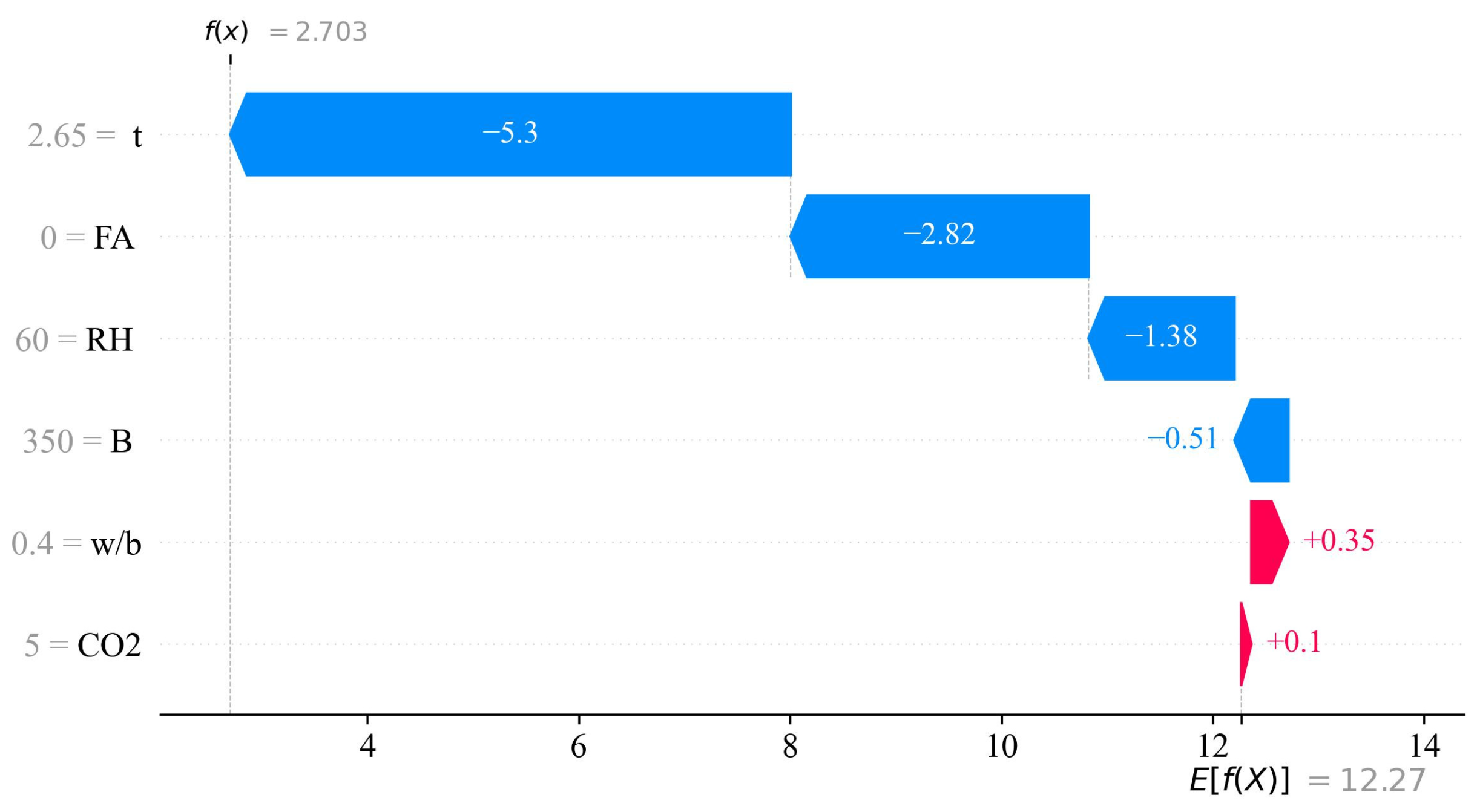
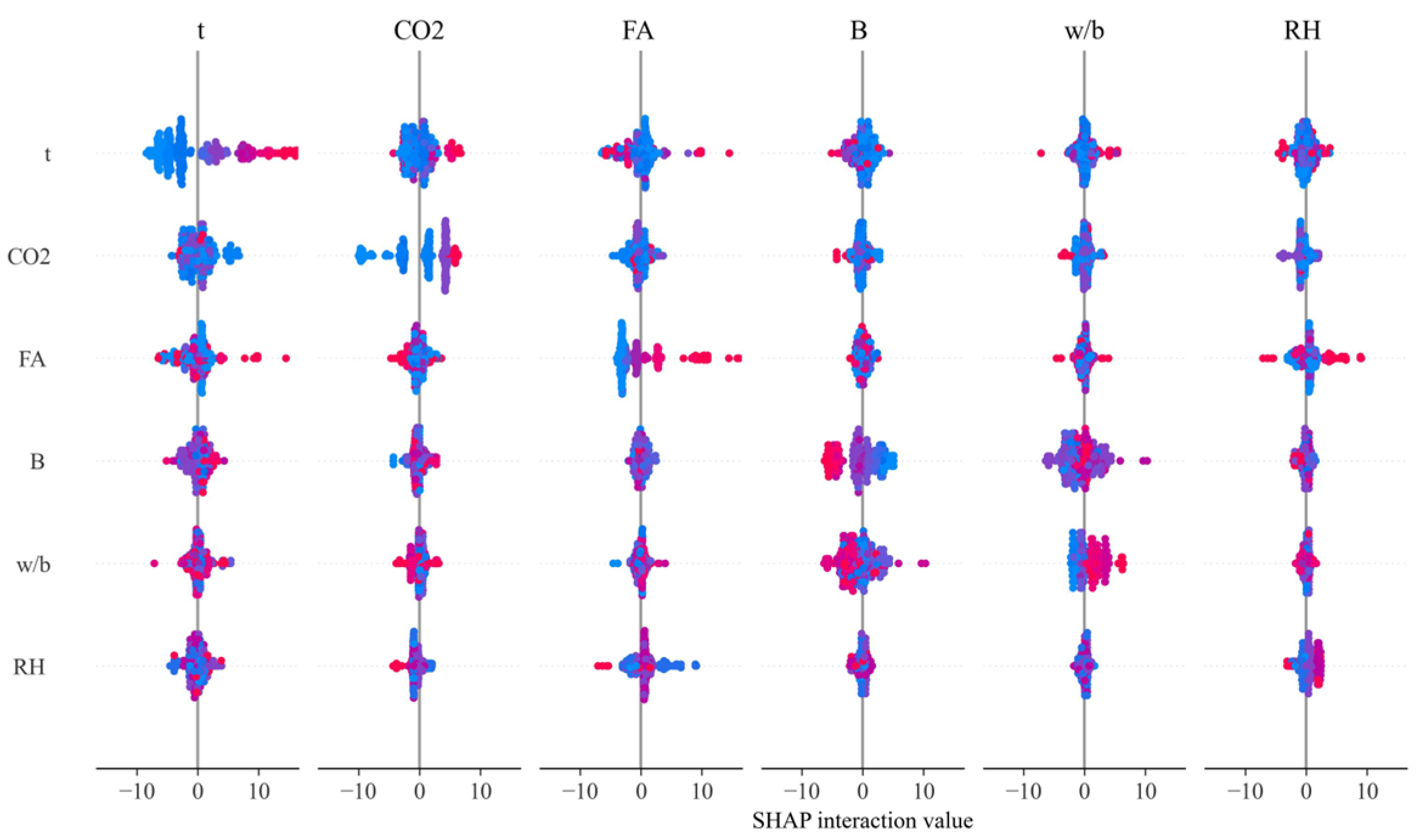
In this paper, the RCFF model was analyzed for SHAP interpretation through three levels. Based on the SHAP analysis, it was found that exposure time and CO₂ concentration were the most important factors affecting the depth of carbonation, with exposure time contributing the highest SHAP value. This indicates that prolonged exposure significantly deepens the carbonation. In addition, FA and B also had a significant effect on the depth of carbonation, while w/b and RH had the second highest but still not negligible effect. SHAP interaction analysis revealed a significant interaction between FA, CO_2, and t, which suggests that fly ash admixture and CO₂ concentration intensified the effect of carbonation under prolonged exposure. Whereas RH interacted weakly with other variables, relative humidity was more inclined to influence the carbonation process alone.

Although the superiority of RCFF is demonstrated in this paper, the generalization ability of the model is still limited by the size and quality of the dataset, and the dataset needs to be further expanded in the future to enhance the applicability of the model. Meanwhile, combining physical mechanisms with data-driven methods to construct a hybrid model is expected to further improve the scientific rationality of the prediction results.

References

1. Papadakis, V.G.; Vayenas, C.G.; Fardis, M.N. Fundamental Modeling and Experimental Investigation of Concrete Carbonation. Mater. J. 1991, 88, 363–373. [Google Scholar]
2. Papadakis, V.G.; Vayenas, C.G.; Fardis, M.N. Physical and Chemical Characteristics Affecting the Durability of Concrete. Mater. J. 1991, 88, 186–196. [Google Scholar]
3. Amorim, P.; de Brito, J.; Evangelista, L. Concrete Made with Coarse Concrete Aggregate: Influence of Curing on Durability. Mater. J. 2012, 109, 195–204. [Google Scholar]
4. Wierig, H. Longtime studies on the carbonation on concrete under normal outdoor exposure. In Proceedings of the Rilem Seminar Durability of Concrete Structures under Normal Outdoor Exposure, Hannover, Germany, 26–29 March 1984; pp. 239–249. [Google Scholar]
5. Bahador, S.D.; Cahyadi, J.H. Modelling of carbonation of PC and blended cement concrete. IES J. Part A Civ. Struct. Eng. 2009, 2, 59–67. [Google Scholar] [CrossRef]
6. Ngala, V.; Page, C. Effects of carbonation on pore structure and diffusional properties of hydrated cement pastes. Cem. Concr. Res. 1997, 27, 995–1007. [Google Scholar] [CrossRef]
7. Ahmad, S. Reinforcement corrosion in concrete structures, its monitoring and service life prediction—A review. Cem. Concr. Compos. 2003, 25, 459–471. [Google Scholar] [CrossRef]
8. Page, C.; Treadaway, K. Aspects of the electrochemistry of steel in concrete. Nature 1982, 297, 109–115. [Google Scholar] [CrossRef]
9. Leek, D.S. The passivity of steel in concrete. Q. J. Eng. Geol. Hydrogeol. 1991, 24, 55–66. [Google Scholar] [CrossRef]
10. Ghods, P.; Isgor, O.B.; Bensebaa, F.; Kingston, D. Angle-resolved XPS study of carbon steel passivity and chloride-induced depassivation in simulated concrete pore solution. Corros. Sci. 2012, 58, 159–167. [Google Scholar] [CrossRef]
11. Jiang, L.; Lin, B.; Cai, Y. A model for predicting carbonation of high-volume fly ash concrete. Cem. Concr. Res. 2000, 30, 699–702. [Google Scholar] [CrossRef]
12. Shen, W.; Cao, L.; Li, Q.; Zhang, W.; Wang, G.; Li, C. Quantifying CO2 emissions from China’s cement industry. Renew. Sustain. Energy Rev. 2015, 50, 1004–1012. [Google Scholar] [CrossRef]
13. von Greve-Dierfeld, S.; Lothenbach, B.; Vollpracht, A.; Wu, B.; Huet, B.; Andrade, C.; Medina, C.; Thiel, C.; Gruyaert, E.; Vanoutrive, H.; et al. Understanding the carbonation of concrete with supplementary cementitious materials: A critical review by RILEM TC 281-CCC. Mater. Struct. 2020, 53, 136. [Google Scholar] [CrossRef]
14. Zhang, D.; Cai, X.; Shao, Y. Carbonation curing of precast fly ash concrete. J. Mater. Civ. Eng. 2016, 28, 04016127. [Google Scholar] [CrossRef]
15. Zhang, J.; Cheng, M.; Zhu, J. Carbonation depth model and prediction of hybrid fiber fly ash concrete. Adv. Civ. Eng. 2020, 2020, 9863963. [Google Scholar] [CrossRef]
16. Carević, V.; Ignjatović, I.; Dragaš, J. Model for practical carbonation depth prediction for high volume fly ash concrete and recycled aggregate concrete. Constr. Build. Mater. 2019, 213, 194–208. [Google Scholar] [CrossRef]
17. Te Liang, M.; Qu, W.J.; Liang, C.-H. Mathematical modeling and prediction method of concrete carbonation and its applications. J. Mar. Sci. Technol. 2002, 10, 128–135. [Google Scholar] [CrossRef]
18. Bonnet, S.; Balayssac, J.-P. Combination of the Wenner resistivimeter and Torrent permeameter methods for assessing carbonation depth and saturation level of concrete. Constr. Build. Mater. 2018, 188, 1149–1165. [Google Scholar] [CrossRef]
19. Tuutti, K. Corrosion of Steel in Concrete. Ph.D. Thesis, Swedish Cement and Concrete Research Institute, Stockholm, Sweden, 1982. [Google Scholar]
20. Long, W.; Bao, Z.; Chen, K.; Ng, S.T.; Wuni, I.Y. Developing an integrative framework for digital twin applications in the building construction industry: A systematic literature review. Adv. Eng. Inform. 2024, 59, 102346. [Google Scholar] [CrossRef]
21. Liu, W.; Li, A.; Fang, W.; Love, P.E.; Hartmann, T.; Luo, H. A hybrid data-driven model for geotechnical reliability analysis. Reliab. Eng. Syst. Saf. 2023, 231, 108985. [Google Scholar] [CrossRef]
22. Hou, H.; Liu, C.; Wei, R.; He, H.; Wang, L.; Li, W. Outage duration prediction under typhoon disaster with stacking ensemble learning. Reliab. Eng. Syst. Saf. 2023, 237, 109398. [Google Scholar] [CrossRef]
23. Londhe, S.; Kulkarni, P.; Dixit, P.; Silva, A.; Neves, R.; de Brito, J. Tree based approaches for predicting concrete carbonation coefficient. Appl. Sci. 2022, 12, 3874. [Google Scholar] [CrossRef]
24. Kellouche, Y.; Boukhatem, B.; Ghrici, M.; Tagnit-Hamou, A. Exploring the major factors affecting fly-ash concrete carbonation using artificial neural network. Neural Comput. Appl. 2019, 31, 969–988. [Google Scholar] [CrossRef]
25. Akpinar, P.; Uwanuakwa, I.D. Intelligent prediction of concrete carbonation depth using neural networks. Bull. Transilv. Univ. Bras. Ser. III Math. Comput. Sci. 2016, 9, 99–108. [Google Scholar]
26. Huang, X.; Liu, W.; Guo, Q.; Tan, J. Prediction method for the dynamic response of expressway lateritic soil subgrades on the basis of Bayesian optimization CatBoost. Soil Dyn. Earthq. Eng. 2024, 186, 108943. [Google Scholar] [CrossRef]
27. Kumar, N.; Prakash, S.; Ghani, S.; Gupta, M.; Saharan, S. Data-driven machine learning approaches for predicting permeability and corrosion risk in hybrid concrete incorporating blast furnace slag and fly ash. Asian J. Civ. Eng. 2024, 25, 3263–3275. [Google Scholar] [CrossRef]
28. Wu, J.; Zhao, G.; Wang, M.; Xu, Y.; Wang, N. Concrete carbonation depth prediction model based on a gradient-boosting decision tree and different metaheuristic algorithms. Case Stud. Constr. Mater. 2024, 21, e03864. [Google Scholar] [CrossRef]
29. Luo, L.; Chen, X. Integrating piecewise linear representation and weighted support vector machine for stock trading signal prediction. Appl. Soft Comput. 2013, 13, 806–816. [Google Scholar] [CrossRef]
30. Asteris, P.G.; Skentou, A.D.; Bardhan, A.; Samui, P.; Pilakoutas, K. Predicting concrete compressive strength using hybrid ensembling of surrogate machine learning models. Cem. Concr. Res. 2021, 145, 106449. [Google Scholar] [CrossRef]
31. Cook, R.; Lapeyre, J.; Ma, H.; Kumar, A. Prediction of compressive strength of concrete: Critical comparison of performance of a hybrid machine learning model with standalone models. J. Mater. Civ. Eng. 2019, 31, 04019255. [Google Scholar] [CrossRef]
32. Wang, M.; Mitri, H.S.; Zhao, G.; Wu, J.; Xu, Y.; Liang, W.; Wang, N. Performance comparison of several explainable hybrid ensemble models for predicting carbonation depth in fly ash concrete. J. Build. Eng. 2024, 98, 111246. [Google Scholar] [CrossRef]
33. Huo, Z.; Wang, L.; Huang, Y. Predicting carbonation depth of concrete using a hybrid ensemble model. J. Build. Eng. 2023, 76, 107320. [Google Scholar] [CrossRef]
34. Han, T.; Siddique, A.; Khayat, K.; Huang, J.; Kumar, A. An ensemble machine learning approach for prediction and optimization of modulus of elasticity of recycled aggregate concrete. Constr. Build. Mater. 2020, 244, 118271. [Google Scholar] [CrossRef]
35. Meng, S.; Shi, Z.; Xia, C.; Zhou, C.; Zhao, Y. Exploring LightGBM-SHAP: Interpretable predictive modeling for concrete strength under high temperature conditions. Structures 2025, 71, 108134. [Google Scholar] [CrossRef]
36. Breiman, L. Bagging predictors. Mach. Learn. 1996, 24, 123–140. [Google Scholar] [CrossRef]
37. Schapire, R.E. The strength of weak learnability. Mach. Learn. 1990, 5, 197–227. [Google Scholar] [CrossRef]
38. Liu, Z.; Zhang, Y.; Abedin, M.Z.; Wang, J.; Yang, H.; Gao, Y.; Chen, Y. Profit-driven fusion framework based on bagging and boosting classifiers for potential purchaser prediction. J. Retail. Consum. Serv. 2024, 79, 103854. [Google Scholar] [CrossRef]
39. Chang, C.F.; Chen, J.W. The experimental investigation of concrete carbonation depth. Cem. Concr. Res. 2006, 36, 1760–1767. [Google Scholar] [CrossRef]
40. Cui, H.; Tang, W.; Liu, W.; Dong, Z.; Xing, F. Experimental study on effects of CO2 concentrations on concrete carbonation and diffusion mechanisms. Constr. Build. Mater. 2015, 93, 522–527. [Google Scholar] [CrossRef]
41. Balayssac, J.P.; Détriché, C.H.; Grandet, J. Effects of curing upon carbonation of concrete. Constr. Build. Mater. 1995, 9, 91–95. [Google Scholar] [CrossRef]
42. Roziere, E.; Loukili, A.; Cussigh, F. A performance based approach for durability of concrete exposed to carbonation. Constr. Build. Mater. 2009, 23, 190–199. [Google Scholar] [CrossRef]
43. Hussain, S.; Bhunia, D.; Singh, S.B. Comparative study of accelerated carbonation of plain cement and fly-ash concrete. J. Build. Eng. 2017, 10, 26–31. [Google Scholar] [CrossRef]
44. Younsi, A.; Turcry, P.; Aït-Mokhtar, A.; Staquet, S. Accelerated carbonation of concrete with high content of mineral additions: Effect of interactions between hydration and drying. Cem. Concr. Res. 2013, 43, 25–33. [Google Scholar] [CrossRef]
45. Turcry, P.; Oksri-Nelfia, L.; Younsi, A.; AT-Mokhtar, A. Analysis of an accelerated carbonation test with severe preconditioning. Cem. Concr. Res. 2014, 57, 70–78. [Google Scholar] [CrossRef]
46. Chen, Y.; Liu, P.; Yu, Z. Effects of Environmental Factors on Concrete Carbonation Depth and Compressive Strength. Materials 2018, 11, 2167. [Google Scholar] [CrossRef]
47. Khunthongkeaw, J.; Tangtermsirikul, S.; Leelawat, T. A study on carbonation depth prediction for fly ash concrete. Constr. Build. Mater. 2006, 20, 744–753. [Google Scholar] [CrossRef]
48. Huang, C.; Geng, G.; Lu, Y.; Bao, G.; Lin, Z. Carbonation depth research of concrete with low-volume fly ash. In Proceedings of the International Conference on Mechanical Engineering and Green Manufacturing (MEGM 2012), Chongqing, China, 16–18 March 2012. [Google Scholar]
49. Gao, Y.; Cheng, L.; Gao, Z.; Guo, S. Effects of different mineral admixtures on carbonation resistance of lightweight aggregate concrete. Constr. Build. Mater. 2013, 43, 506–510. [Google Scholar] [CrossRef]
50. Zhao, Q.; He, X.; Zhang, J.; Jiang, J. Long-age wet curing effect on performance of carbonation resistance of fly ash concrete. Constr. Build. Mater. 2016, 127, 577–587. [Google Scholar] [CrossRef]
51. Kurda, R.; Brito, J.D.; Silvestre, J.D. Carbonation of concrete made with high amount of fly ash and recycled concrete aggregates for utilization of CO2. J. CO2 Util. 2019, 29, 12–19. [Google Scholar] [CrossRef]
52. Lu, C.F.; Wang, W.; Li, Q.T.; Hao, M.; Xu, Y. Effects of micro-environmental climate on the carbonation depth and the pH value in fly ash concrete. J. Clean. Prod. 2018, 181, 309–317. [Google Scholar] [CrossRef]
53. Atis, C.D. Accelerated carbonation and testing of concrete made with fly ash. Constr. Build. Mater. 2003, 17, 147–152. [Google Scholar] [CrossRef]
54. Tu, L.Q.; Xu, W.B.; Chen, W. Carbonation of Fly Ash Concrete and Micro-Hardness Analysis. Adv. Mater. Res. 2011, 378–379, 56–59. [Google Scholar]
55. Felix, E.F.; Carrazedo, R.; Possan, E. Carbonation model for fly ash concrete based on artificial neural network: Development and parametric analysis. Constr. Build. Mater. 2021, 266, 121050. [Google Scholar] [CrossRef]
56. Papadakis, V.G. Effect of fly ash on Portland cement systems Part I. Low-calcium fly ash. Cem. Concr. Res. 1999, 29, 1727–1736. [Google Scholar] [CrossRef]
57. Dunlop, P.; Smith, S. Estimating key characteristics of the concrete delivery and placement process using linear regression analysis. Civ. Eng. Environ. Syst. 2003, 20, 273–290. [Google Scholar] [CrossRef]
58. Breiman, L. Random forests. Mach. Learn. 2001, 45, 5–32. [Google Scholar] [CrossRef]
59. Xia, Y.; Zhao, J.; He, L.; Li, Y.; Niu, M. A novel tree-based dynamic heterogeneous ensemble method for credit scoring. Expert Syst. Appl. 2020, 159, 113615. [Google Scholar] [CrossRef]
60. Prokhorenkova, L.; Gusev, G.; Vorobev, A.; Dorogush, A.V.; Gulin, A. CatBoost: Unbiased boosting with categorical features. In Proceedings of the 32nd Conference on Neural Information Processing Systems (NIPS), Montreal, QC, Canada, 3–8 December 2018. [Google Scholar]
61. Dorogush, A.V.; Ershov, V.; Gulin, A. CatBoost: Gradient boosting with categorical features support. arXiv 2018, arXiv:181011363. [Google Scholar]
62. Avrizal, R.; Wibowo, A.; Yuniarti, A.S.; Sandy, D.A.; Prihandani, K. Analysis Comparison of The Classification Data Mining Method to Predictthe Decisions of Potential Customer Insurance. Int. J. Comput. Tech. 2018, 5, 15–20. [Google Scholar]
63. Alam, M.S.; Sultana, N.; Hossain, S.Z. Bayesian optimization algorithm based support vector regression analysis for estimation of shear capacity of FRP reinforced concrete members. Appl. Soft Comput. 2021, 105, 107281. [Google Scholar] [CrossRef]
64. Daneshvar, K.; Moradi, M.J.; Khaleghi, M.; Rezaei, M.; Farhangi, V.; Hajiloo, H. Effects of impact loads on heated-and-cooled reinforced concrete slabs. J. Build. Eng. 2022, 61, 105328. [Google Scholar] [CrossRef]
65. Wang, M.; Zhao, G.; Liang, W.; Wang, N. A comparative study on the development of hybrid SSA-RF and PSO-RF models for predicting the uniaxial compressive strength of rocks. Case Stud. Constr. Mater. 2023, 18, e02191. [Google Scholar] [CrossRef]
66. Rui, J. Exploring the association between the settlement environment and residents’ positive sentiments in urban villages and formal settlements in Shenzhen. Sustain. Cities Soc. 2023, 98, 104851. [Google Scholar] [CrossRef]
67. Nguyen, M.H.; Mai, H.-V.T.; Trinh, S.H.; Ly, H.-B. A comparative assessment of tree-based predictive models to estimate geopolymer concrete compressive strength. Neural Comput. Appl. 2023, 35, 6569–6588. [Google Scholar] [CrossRef]
68. Li, Z. Extracting spatial effects from machine learning model using local interpretation method: An example of SHAP and XGBoost. Comput. Environ. Urban Syst. 2022, 96, 101845. [Google Scholar] [CrossRef]
69. Kim, C.-M.; Jaffari, Z.H.; Abbas, A.; Chowdhury, M.F.; Cho, K.H. Machine learning analysis to interpret the effect of the photocatalytic reaction rate constant (k) of semiconductor-based photocatalysts on dye removal. J. Hazard. Mater. 2024, 465, 132995. [Google Scholar] [CrossRef] [PubMed]
70. Sun, Z.; Li, Y.; Li, Y.; Su, L.; He, W. Investigation on compressive strength of coral aggregate concrete: Hybrid machine learning models and experimental validation. J. Build. Eng. 2024, 82, 108220. [Google Scholar] [CrossRef]
71. Rahmani, P.; Gholami, H.; Golzari, S. An interpretable deep learning model to map land subsidence hazard. Environ. Sci. Pollut. Res. 2024, 31, 17448–17460. [Google Scholar] [CrossRef]
72. Hastie, T. The Elements of Statistical Learning: Data Mining, Inference, and Prediction; Springer: New York, NY, USA, 2009. [Google Scholar]
73. Tzeng, G.-H.; Huang, J.-J. Multiple Attribute Decision Making: Methods and Applications; CRC Press: Boca Raton, FL, USA, 2011. [Google Scholar]
74. Han, J.; Pei, J.; Tong, H. Data Mining: Concepts and Techniques; Morgan Kaufmann: Burlington, MA, USA, 2022. [Google Scholar]
75. Liu, P.; Yu, Z.; Chen, Y. Carbonation depth model and carbonated acceleration rate of concrete under different environment. Cem. Concr. Compos. 2020, 114, 103736. [Google Scholar] [CrossRef]
Figure 1. Detailed references and pertinent information about database [11,24,39,40,41,42,43,44,45,46,47,48,49,50,51,52,53,54].
Buildings 15 01349 g001
Figure 2. Scatter plot of input features.
Buildings 15 01349 g002
Figure 3. Correlation matrix.
Buildings 15 01349 g003
Figure 4. Detailed RCFF process.
Buildings 15 01349 g004
Figure 5. MAE versus iteration for the seven models.
Buildings 15 01349 g005
Figure 6. Predictive performance of models.
Buildings 15 01349 g006
Figure 7. Predictive performance of models.
Buildings 15 01349 g007
Figure 8. Taylor diagram.
Buildings 15 01349 g008
Figure 9. Results of the global importance analysis of the input features for RCFF.
Buildings 15 01349 g009
Figure 10. Local interpretation of sample for carbonation depth for RCFF.
Buildings 15 01349 g010
Figure 11. SHAP interaction value matrix diagram.
Buildings 15 01349 g011
Figure 12. The results of feature importance analysis of the input features for the RCFF.
Buildings 15 01349 g012