Abstract
The location of housing has a significant influence on its pricing. Generally, spatial self-correlation and spatial heterogeneity phenomena affect housing price data. Additionally, time is a crucial factor in housing price modeling, as it helps understand market trends and fluctuations. Currency market fluctuations also directly affect housing prices. Therefore, in addition to the physical features of the property, such as the area of the residential unit and building age, the rate of exchange (dollar price) is added to the independent variable set. This study used the real estate transaction records from Iran’s registration system, covering February, May, August, and November in 2017–2019. Initially, 7464 transactions were collected, but after preprocessing, the dataset was refined to 7161 records. Unlike feedforward neural networks, the generalized regression neural network does not converge to local minimums, so in this research, the Geographically, Temporally, and Characteristically Weighted Generalized Regression Neural Network (GTCW-GRNN) for housing price modeling was developed. In addition to being able to model the spatial–time heterogeneity available in observations, this algorithm is accurate and faster than MLR, GWR, GRNN, and GCW-GRNN. The average index of the adjusted coefficient of determination in other methods, including the MLR, GWR, GTWR, GRNN, GCW-GRNN, and the proposed GTCW-GRNN in different modes of using Euclidean or travel distance and fixed or adaptive kernel was equal to 0.760, 0.797, 0.854, 0.777, 0.774, and 0.813, respectively, which showed the success of the proposed GTCW-GRNN algorithm. The results showed the importance of the variable of the dollar and the area of housing significantly.
1. Introduction
Property price modeling requires samples to be homogeneous and (mutually) independent. Observational independence is a strong assumption in issues that beg the locational component. According to the first law of geography, the connection between adjacent phenomena is stronger than that between distanced ones [1]. In other words, if two independent samples lie close to each other, the assumption of their independence would not be strong anymore. The housing market is an excellent example of this law. For example, two completely identical apartments located in two different neighborhoods do not have the same price. As another example, an uptown apartment has a higher price than its equivalent downtown.
Generally, we face spatial self-correlation and spatial heterogeneity phenomena. Spatial self-correlation means the data exhibit a specific pattern in their spatial dispersion. In other words, if there is a significant relationship between two variables observed in two different locations, then they depend on each other’s spatial position [2]. Spatially heterogeneous means that the anticipated coefficients in a regression relation are not the same for each variable in different locations. Time, in addition to location, is a defining factor in housing price modeling.
Belke and Keil [3] empirically observed that with the change in eurozone money shares, the price of residential property increased in 30 German cities. Therefore, due to the fact that in Iran, the ratio of dollars to rials is always changing, dollars were added to other independent variables to model housing prices, as the US dollar is the main currency in the Iranian housing market. Given the observed correlation between inflation indices and USD exchange rates, the dollar price was selected as the independent variable for housing price modeling, as it effectively captures both currency fluctuations and inflationary effects within the study period. Accordingly, this study incorporated external and economic factors influencing housing prices, including the exchange rate (USD price) and population density. Moreover, other influential independent variables were identified after considering previous studies and related data. In this regard, to measure accessibility to urban services, the Euclidean distance from each property to sports centers, healthcare facilities, religious sites, green spaces, public transit stations (including buses, subways, and taxis), and highways were computed. Furthermore, property safety was assessed using the Euclidean distance to the nearest active and inactive fault lines in Tehran. These factors, combined with other physical housing characteristics, can substantially enhance the housing price modeling process.
In this study, we first establish a linear geographically and temporally weighted regression called GTWR and compare it to a non-linear regression in order to ascertain whether there is a linear relationship between the independent variables and the dimensions of space and time. Chen et al. [4] used a geographical and temporal neural network weighted regression (GTNNWR) model for PM2.5 modelling that can model the non-linear relationship between independent variables and spatiotemporal dimensions. This model is based on back-propagation neural networks (BPNNs). Martinez-Blanco et al. [5] compared BPNN and GRNN models. They achieved better results in their modeling with the GRNN method compared those who used the BPNN method. Wu et al. [6] developed the GTNNWR model, which is based on the BPNN model. Considering that the GRNN model is simpler, faster, and more accurate compared to the BPNN model, which is contrary to its high capability in modeling, in this research, a GRNN model was developed. Also, Li et al. [7] modeled PM2.5 using the GTW-GRNN method. But in their model, the weight of characteristic variables is not considered, and therefore it is not a suitable method for modeling housing price, which is highly dependent on its independent variables. For this purpose, the GTCW-GRNN model was introduced, for which there is a non-linear relationship between the independent variables and spatiotemporal dimensions.
Highlights of this study are categorized as follows:
- Using the GRNN model and accounting for the geographical and temporal heterogeneities in the housing price data, the GCW-GRNN and GTCW-GRNN models were developed and introduced to represent the existing non-linear correlations between dependent and independent variables.
- Analyzing travel distance in addition to Euclidean distance in housing price modeling.
- Examining the impact of the amount of access to urban services on estimating the home price, such as the distance from sports, medical, religious, and educational facilities, etc., and investigating the external and economic variables impacting the housing price, such as the exchange rate (dollar price).
2. Literature Review
According to the first law of geography, closer things are more similar [1]. This principle can be extended to the housing price anticipation problem. The spatial development method presented by Casetti [8] was the first regression model that considered spatial heterogeneity [9]. However, its disadvantage is the way of determining the type of the relationship of parameters using the location coordinates of the observations. Since then, various models have been developed, and the most popular one is Geographically Weighted Regression (GWR). The GWR model has attracted much attention in recent years, as a result of which different models have been developed [10]. In housing price modeling, some variables have different effects in different locations, like proximity to recreation–commercial centers, whilst the impact of the rest of the variables is fixed all over the study field. Based on this idea, Brunsdon et al. [11] presented Multiscale Geographically Weighted Regression (MGWR) using the Back-fitting method, where the coefficients of local/global variables are calculated separately [12].
The Geographical Bandwidth (GB) is the same for the applied variables, while the scale effect of them is not the same. Therefore, Fotheringham et al. [13] introduced Multiscale Geographically Weighted Regression (MGWR) and modeled the different scale effects in variables [14]. It is better to replace Travel Distance (TD) with Euclidean Distance (ED) in GWR. Lu et al. [15] improved the coefficient of determination by 0.011 using TD in GWR [16]. When sample observations are gathered from different locations and at different times, there is a chance that the anticipated regression relation has different parameters for each location and time. Huang et al. [17] introduced Geographically and Temporally Weighted Regression (GTWR) and examined the spatiotemporal heterogeneity in the housing price data of Calgary city. Considering different scale effects of variables, they proposed Multiscale Geographically and Temporally Weighted Regression (MGTWR). The results indicate its efficiency compared to MGWR and GTWR in modeling housing prices [18]. Distances are defined inside the transportation network in the real world. Considering this, Liu et al. [19] improved the coefficients of determination by 0.013 and 0.024 for GWR and GTWR, respectively.
In addition to time and location dimensions [20,21,22], property physical features (like the age of the building) and the quality of the materials could be used as the third dimension of the weight matrix. Jiang et al. [23] changed the weight matrix in GTWR and provided better results. The results are applied only to training data that affects the model by over-fitting or under-fitting processes. Bidanset et al. [24] proposed Geographically, Temporally, and Characteristically Weighted Regression (GTCWR) [25]. Its disadvantage is using a linear regression model, which cannot handle the non-linear relations between the observations. Li et al. [7] therefore, proposed a “Geographically and Temporally Weighted Generalized Regression Neural Network (GTW-GRNN)” method for modeling Suspended Particle Concentration (SPC). For this method to be used in housing price modeling, considering the physical features of housing is necessary, besides spatiotemporal heterogeneity in the weighting function. In this research, therefore, a Geographically, Temporally, and Characteristically Weighted Generalized Regression Neural Network (GTCW-GRNN) is proposed. Then, housing price modeling was examined in district 5 of Tehran using the proposed model. To train on high-dimensional data, feature selection techniques must be used. The recursive elimination approach was applied in this study to exclude unrelated features and find related ones. In this approach, the learning model is analyzed on all possible feature combinations, and the model’s accuracy (adjusted R2) is assessed on each of these combinations with initial feature pool of 17 variables [26]. Lastly, a feature combination that the learning model performs more accurately is chosen. No explanatory variables were eliminated in OLS, GWR, and GTWR methods using the feature recursive elimination method to choose the appropriate combination of features. However, explanatory variables such as parking lot, type of skeleton used, population density, and distances from urban transportation stations, medical centers, industrial centers, and green spaces were removed in the methods of GRNN, GCW-GRNN, and GTCW-GRNN. The variables of dollar price, multiplication of floor by the elevator, warehouse, area of the residential unit, building age, distance from sports center, and distances from the religious place, educational center, fault, and highway were therefore used in these methods to model housing price. Using both fixed and adaptive kernels together with two types of distance measurement (Euclidean and travel distance) can improve housing price predictions. Fixed kernels work well in city centers with large data quantity, while adaptive kernels are better for outer areas with fewer data. Using both distance types helps because sometimes Euclidean distance matters, while other times actual travel distance along roads is more important—especially in cities like Tehran with complex street layouts. It is also important to compare traditional linear models (like GWR and GTWR) with newer non-linear methods (like GRNN). While linear models show overall trends, they miss local patterns that affect prices. Our new GTCW-GRNN method combines both approaches for more accurate results.
3. Case Study
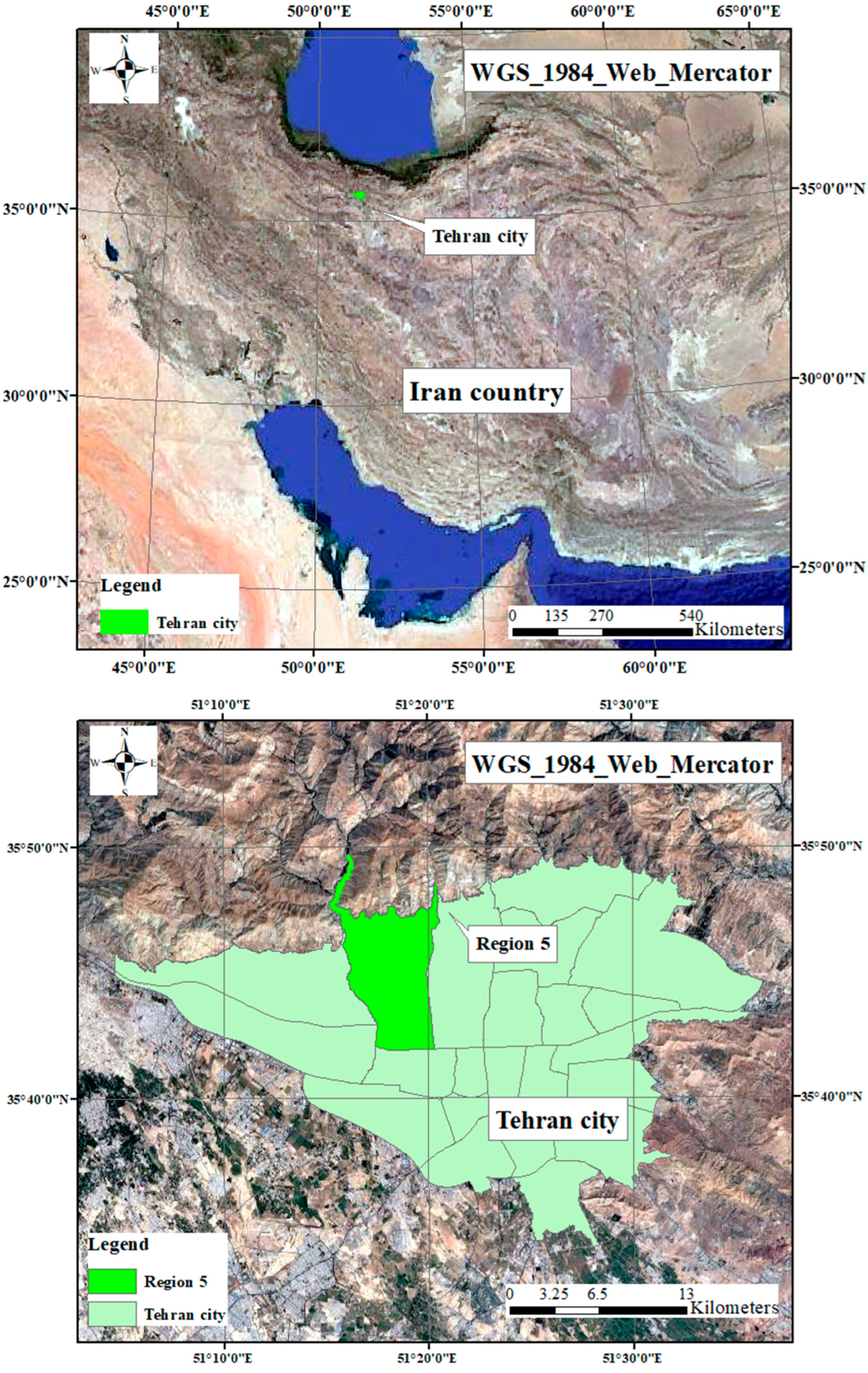
District 5 is one of the most popular districts in Tehran province. It is located between longitudes 51 15′ and 51 20′ east and latitudes 35 41′ and 35 49′ north in the northwest of Tehran. In the 2015 census, its population was 856,565 in 291,665 families. Many of the housing transactions occur in this area. The area of this municipal district is over 59.01 km2 and is ranked as the third-largest district of the capital. Recently, there has been a good opportunity provided for interested people, who are not quite a few, to benefit from this platform and find their appropriate apartment or take advantage of this opportunity. The development indicators are acceptable: indicators such as population density, environmental factors and green spaces, the average age of buildings and types of buildings, per capita in the education sector, proper access to urban infrastructure, the number of public libraries and cultural centers, and even the percentage of people with higher education. The most attractive feature is the reasonable price range. Different people with different tastes can easily find their cases in this district. The urban services in district 5 are desirable. One can easily access different parts of the city using numerous metro stations. According to Tehran real estate stats, one-sixth of transactions are registered in this district. Figure 1 shows the location of this region.
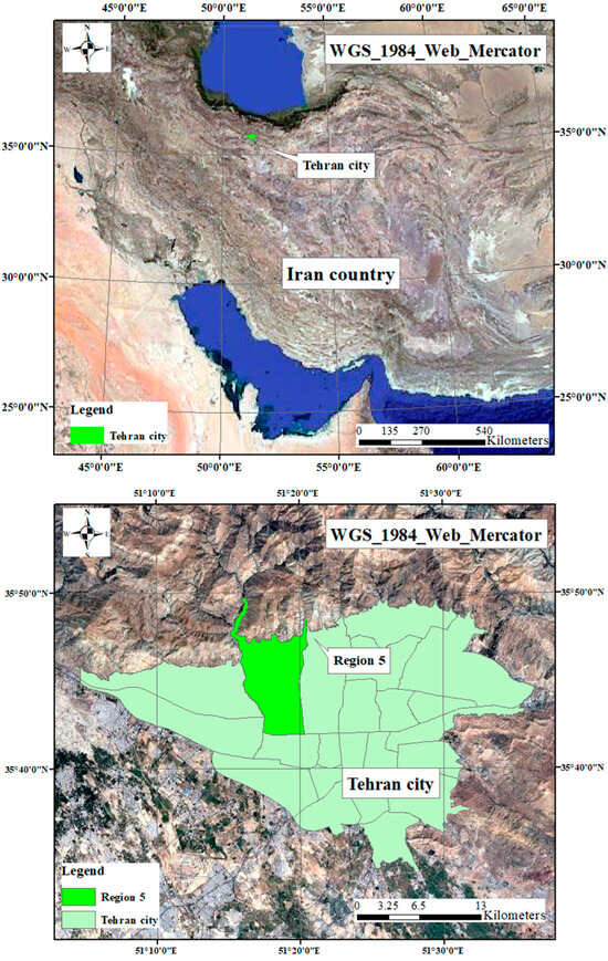
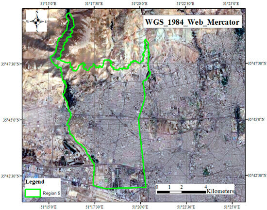
Figure 1.
The location of Tehran and our case study region.
4. Proposed Methodology
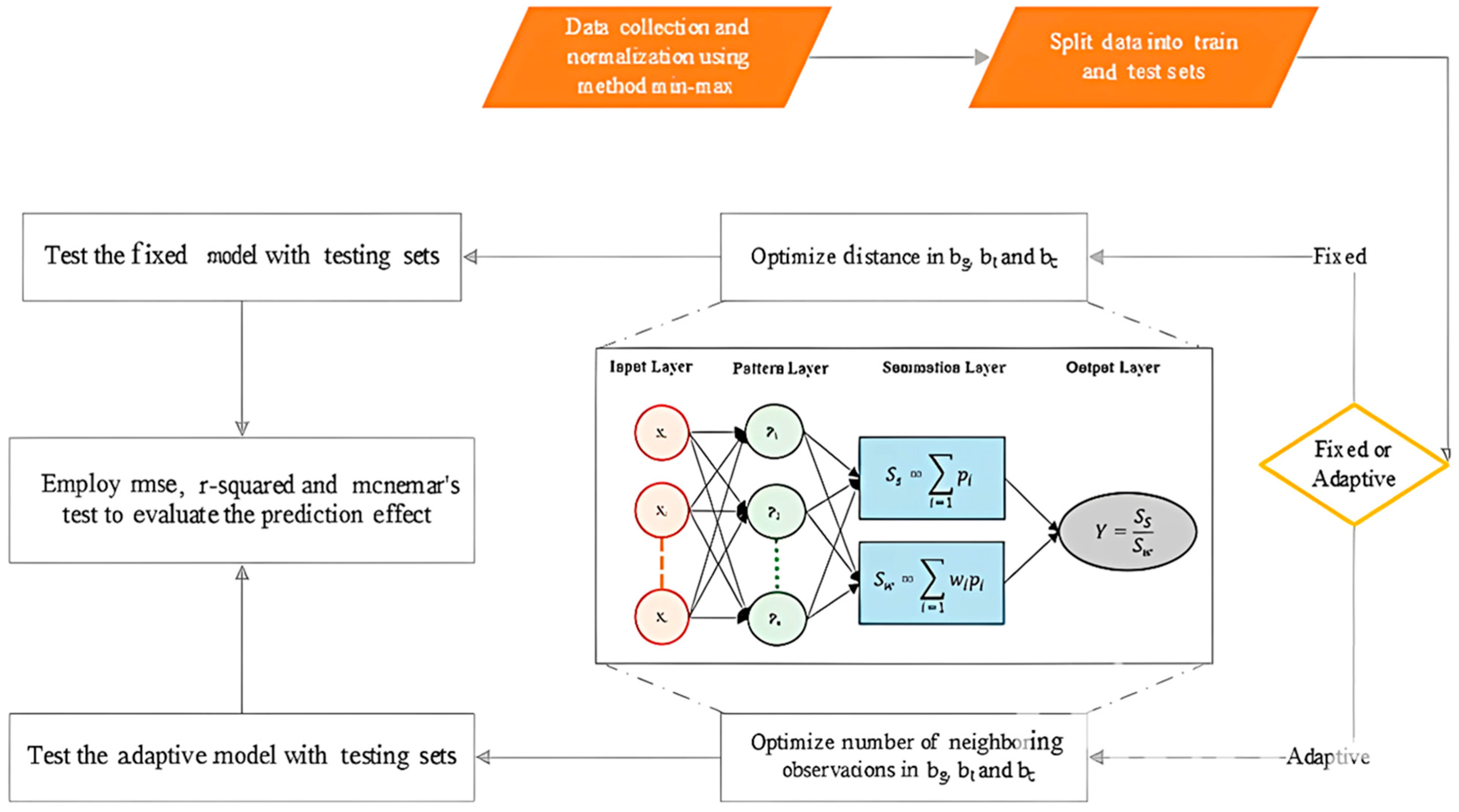
Generalized Regression Neural Network (GRNN) is an advanced supervised neural network engendered in 1991 to estimate continuous functions [27]. In addition to its simplicity and speed in approximation, this algorithm, unlike neural networks with back-propagation error, does not converge into local minimums and there is no need for continuous training [28]. This algorithm is based on non-linear regression theory and addresses the possible non-linear relations among the observations. This algorithm allows for forming a level of linear or non-linear regression from dependent or independent variables [29]. In summary, the structure of the GRNN network comprises four layers: input layer, pattern layer, aggregate layer, and output layer. The first layer provides the inputs to the network. All neurons of this layer are connected to all neurons of the pattern layer. The pattern layer, which is the same argument in the denominator of Equation (2), provides the related calculations to the transition function (Equation (1)). The number of neurons in this layer equals the number of existing learning patterns. The aggregate layer calculates the integrals used in the denominator and numerator of Equation (2). Finally, the output layer divides the outputs of the previous layer and predicts the outcome of the model [30]. The transition function of the ith neuron in the pattern layer is calculated as follows [30]:
where ||.|| is the Euclidean norm calculator operator, σ indicates the slope of the Gaussian function changes, and Xi is the ith learning pattern vector. The following equation provides the output of the GRNN model [30]:
As Equations (1) and (2) indicate, the point of anticipation is a weighted average of different values of Yi. The impact degree of Yi, in fact, depends on the distance between the training point, anticipation point, and σ parameter [31]. Pai and Wang [32] modeled the housing price in Taichung using this method. They considered the geographical coordinates of the centers of the parcels as an independent variable. Modeling the spatial heterogeneities of the observations requires the geographical coordinates of the centers of the parcels to be used in the transition function, and the geographical distance between the training point and anticipation point to be calculated. Therefore, the more the geographical distance between the training point and the anticipation point decreases, the more it will impact the amount of Y of the anticipation point. Time heterogeneity is calculated similarly by transferring the time distance between the training point and anticipation point into the transition function. Finally, treating the physical features is the same as in the previous two cases. This algorithm is applicable in two forms: fixed kernel and adaptive kernel. In the fixed kernel form, the bandwidth is fixed and, therefore, the number of training points varies in the vicinity of each anticipation point. On the contrary, this is not true in adaptive kernel form [33]. Thus, the transition function used in the GTCW-GRNN algorithm comprises location, time, and featured components in both fixed and adaptive forms. Just as the GRNN model does not converge to local minimums, the GTCW-GRNN model also does not converge to local minimums. These components and their relations are summarized in Table 1.

Table 1.
Components of GTCW-GRNN [33].
The dc, dT, and dG in this relation indicate geographical distance, time distance, and feature distance, respectively. The distance is between the ith training point and the jth anticipation point. The hG represents the locational bandwidth, hT represents the time bandwidth, and finally, hC represents the bandwidth of the physical features of the housing or the standard deviation used in the GRNN algorithm. Thus, the numerator of the transition function in the GTCW-GRNN algorithm, for both fixed and adaptive kernels, is the product of three components of location, time, and feature:
GCW-GRNN algorithm is defined as the same as the GTCW-GRNN algorithm, but there is no time component in the GCW-GRNN algorithm—the transition function is the product of location and feature components. Figure 2 depicts the general form of the GTCW-GRNN algorithm.
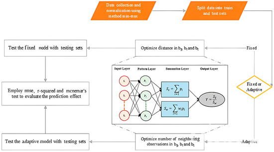
Figure 2.
Proposed GTCW-GRNN algorithm.
R-Squared is used as the main criterion used to compare the accuracy of the models. However, McNemar’s Test is used to investigate the statistical difference in the accuracy of the models. The following equation captures McNemar’s Test [34,35]:
where Z12 represents the statistical difference between the accuracy of the first and second anticipation models; if the difference between the anticipated value and the actual value is smaller than a defined threshold, it will be considered valid. Therefore, f12 represents the number of samples that the first model classified correctly and the second model classified wrongly. Thus, f12 and f21 capture the number of the classified samples on which the first and second anticipation models are not agreed. Z12 specifies a more minor anticipation error (higher accuracy). The negation sign indicates that the results of the second anticipation model are more accurate than those of the first anticipation model. At the 99% confidence level, the difference between the first and second anticipation models is considered as significant, since the amount of |Z12| exceeds 2.575.
5. Dataset
The data were collected using the records of real estate transaction data and retrieved from the real estate registration system of Iran. These data span February, May, August, and November, of 2017, 2018, and 2019 and include 7464 registered transactions. Each point represents a building parcel. In cases where multiple points are assigned to a single parcel, we drew a circle with a diameter equal to the number of points (in centimeters) to avoid any distortions in the calculations. The preprocessing reduced the number of records to 7161. Seventeen influential independent variables were identified after considering previous articles and related data. The dollar price was included in the list of factors used in housing price modeling since the exchange rate influences housing prices in addition to the physical attributes of the housing and the accessibility to urban services [36,37]. Table 2 captures these variables.
Table 2.
Variables used in housing price modeling.
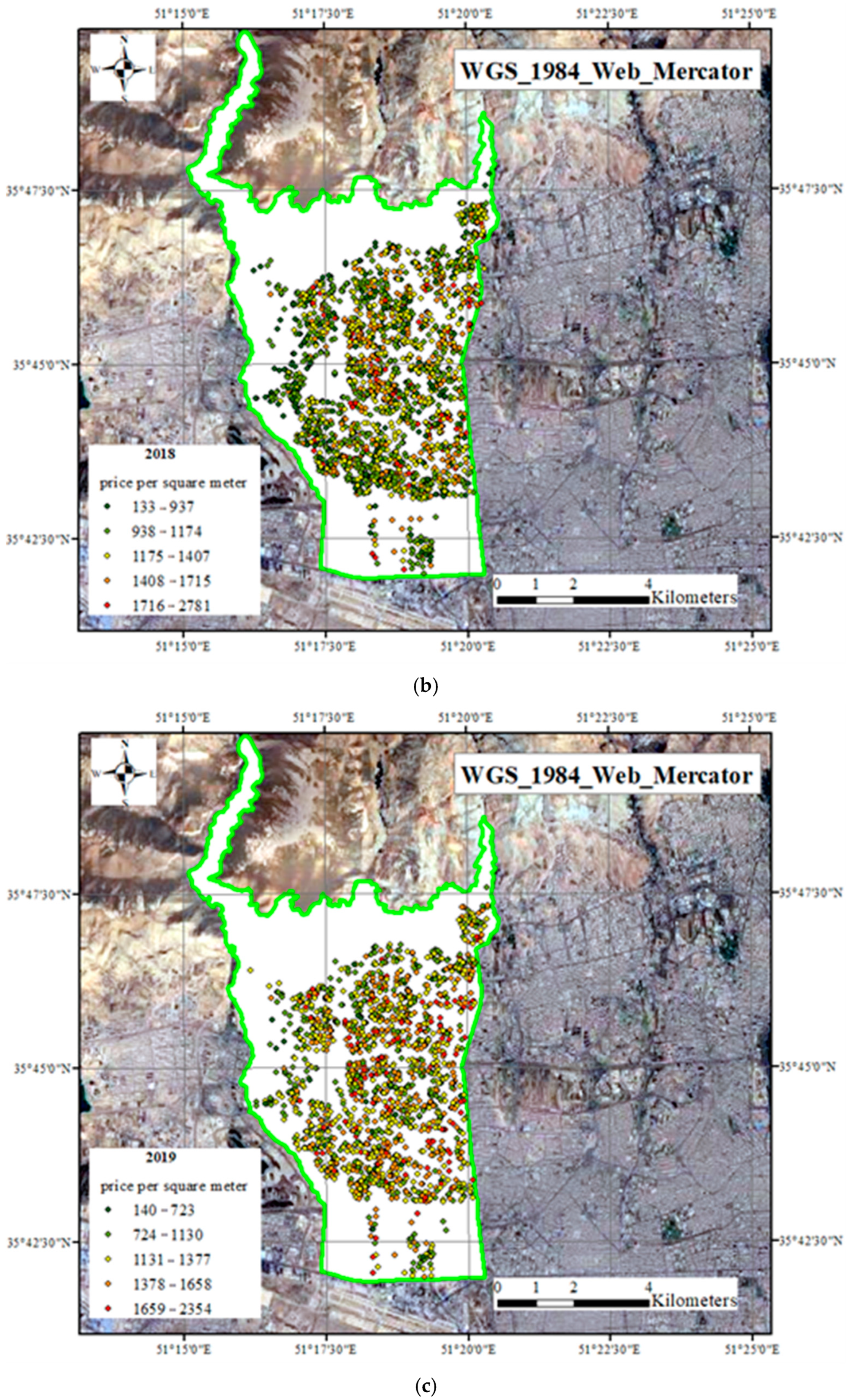
To register the geographical location of the transactions, the “balad.ir” website (routing app) was used to gather the geographical information system data. Figure 3 shows the geographical dispersion of housing transactions prices that occurred in district 5 of Tehran municipality.
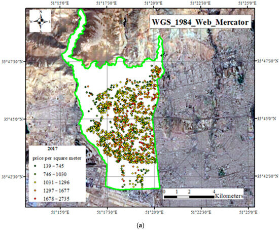
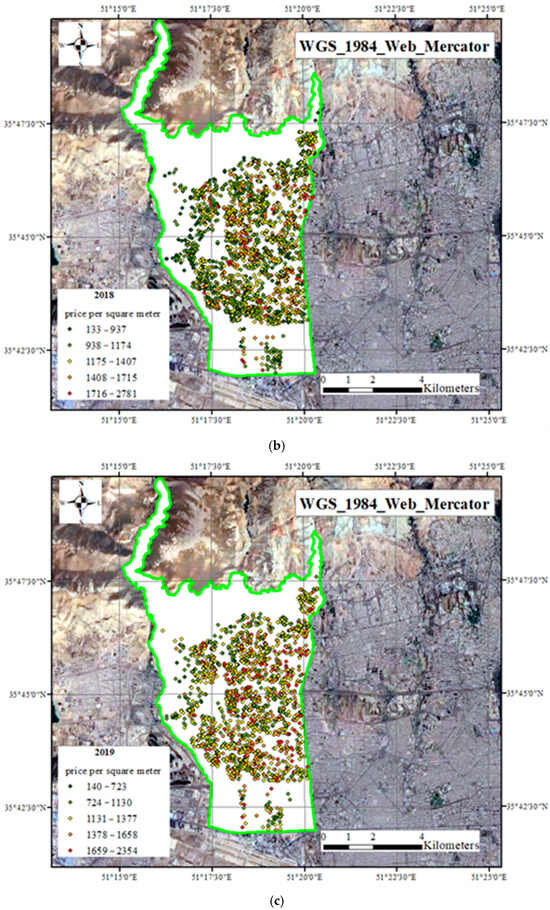
Figure 3.
Geographical distribution of the price per square meter of residential units in 2017 (a), 2018 (b), and 2019 (c) in dollars—district 5 of Tehran municipality.
6. Experimental Results
After preprocessing, 70% of the data were randomly assigned to the train set, and 30% of the data were randomly assigned to the test set. The model is implemented using the Python 3.7 programming language. For those interested in the implementation details, the source code and accompanying documentation are available on GitHub’s web application at https://github.com/SaeidZali/GTCW-GRNN (accessed on 22 April 2024). The repository includes a Jupyter Notebook (v7.1.2). that provides a step-by-step explanation of the main procedures involved in the model’s development and execution.
The parameter tuning for GRNN and GWR models is performed by using the leave-one-out cross validation method, which leaves one record for validation purposes in each stage and uses the rest of the data for training. This method mimics the K-Fold method in which K is considered to be the number of datum records [39]. Since using the leave-one-out cross validation model to find the bandwidth parameters in GTWR, GCW-GRNN, and GTCW-GRNN models is very time-consuming, the golden section search model was used. This method was introduced by Kiefer [40] and recognized by Deb [41] as one of the best single parameter optimization methods. One of the advantages of this method was that 38.2% of the single-variable interval is removed in each loop, and this makes its optimization speed much higher compared to other methods; however, the next challenge was how to use this method for multi-parameter optimization problems. To solve this problem, Chakraborty and Panda [42] introduced an extension of the Golden Section Search method, which is used to optimize multi-parameter problems. They showed that their innovative method works better in comparison with the Nelder–Mead Simplex method. The implementation of their innovative method is difficult for people who do not specialize in mathematics; therefore, in a separate article, Rani et al. [43] introduced Chakraborty and Panda’s [42] innovative method in a simpler way and with MATLAB R2013b code for people who are interested in using this method. Due to the inefficiency of the golden section search method in three-dimensional space [44], Powell’s Conjugate Direction Method was employed for objective function optimization in this study. This derivative-free optimization algorithm operates through orthogonal search directions in the parameter space. The Powell method is particularly efficient for low-dimensional problems (such as three-dimensional cases) and serves as an appropriate choice when calculating the derivative of the objective function is difficult or impossible [45].
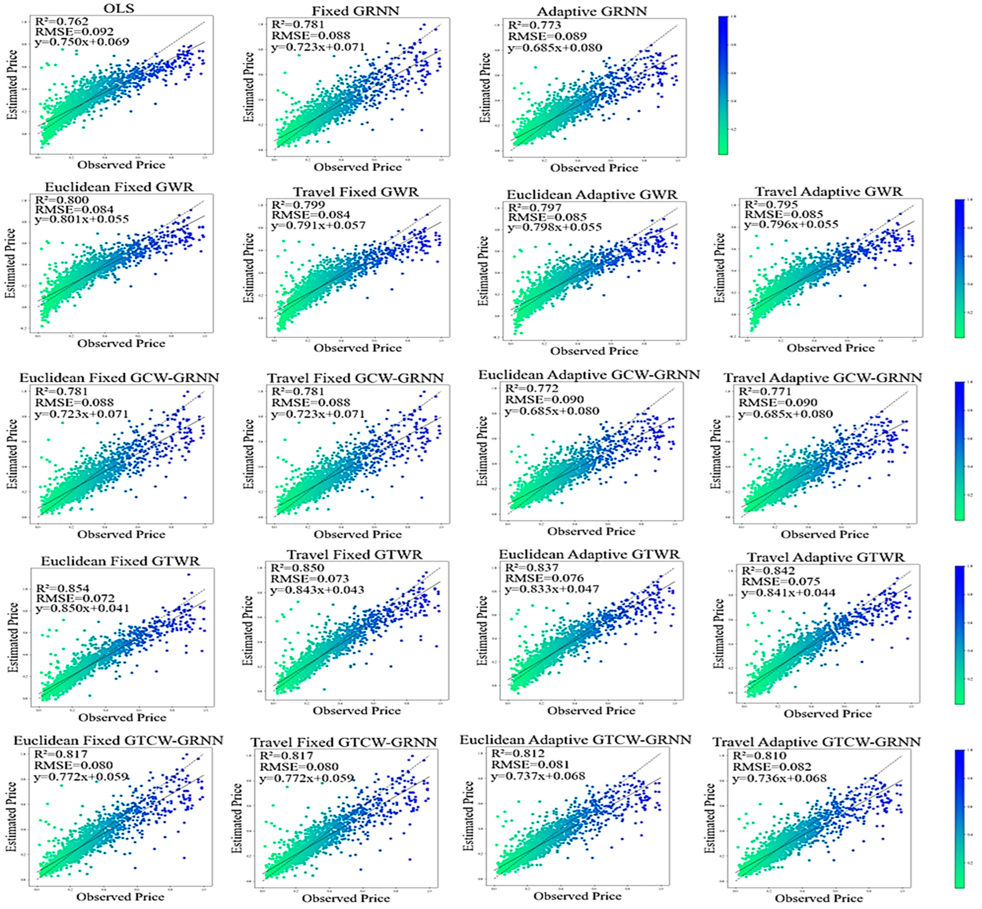
The GRNN, GCW-GRNN, and GTCW-GRNN algorithms are used to investigate the efficiency of the developed models. The heterogeneity of the housing price data in space, time, and physical features is investigated using OLS, GWR, and GTWR algorithms. Figure 4 shows the Root Mean Square Error (RMSE) and R-Squared results for both fixed and adaptive kernel forms, and ED/TD. The fixed form performs better than the adaptive kernel in all cases. The maximum difference of the R-Squared indicator between these two kernels belongs to the Euclidean GTWR algorithm—0.017. The provided results for the GWR, GCW-GRNN, GTWR, and GTCW-GRNN algorithms are almost the same, with a slight difference when the kernel is the same and ED or TD is used. The RMSE and R-Squared indicators in fixed GCW-GRNN and fixed GTCW-GRNN have the same value. In OLS, the R-Squared indicator is 0.762. In GWR, the R-Squared indicator in all fixed, adaptive, ED, or TD is higher compared to the OLS algorithm.
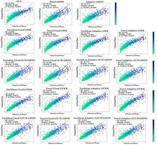
Figure 4.
RMSE and Adjusted R-Squared indicators and related derivatives resulted from OLS and GRNN in housing price modeling.
GTWR, generally, performs better than GWR, and its R-Squared is higher. The average R-Squared captured from different forms of GWR and GTWR is equal to 0.797 and 0.854, respectively. Therefore, compared to OLS, the average R-Squared indicator improved by 0.035 and 0.083 in different forms of GWR and GTWR, respectively. Note that there is spatial and spatiotemporal heterogeneity in the housing price data. The average R-Squared captured from GRNN (fixed and adaptive) is 0.777. Considering the presence of heterogeneity, the average R-Squared indicator is 0.776 and 0.814 in GCW-GRNN and GTCW-GRNN, respectively. In comparison to the GCW-GRNN method, the GRNN algorithm’s mean R-Squared index value is 0.001 greater on average. Additionally, when compared to the GRNN method, the mean value of the R-Squared index in the GTCW-GRNN algorithm is 0.037 greater.
Also, a summary of the results is shown in Figure 5. The coefficient of determination with a value of 0.721 is considered as the zero of the vertical axis of the graph.
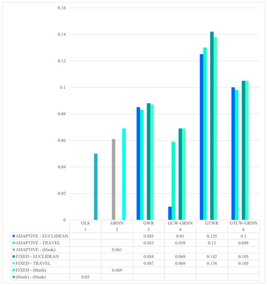
Figure 5.
Summary of the R-Squared (R2) results.
As you can see in Figure 5, better results will be obtained if Euclidean distance and fixed kernel are used in different GWR, GTWR, GCW-GRNN, and GTCW-GRNN methods.
As indicated before, GTWR and GTCW-GRNN models have better performance against other models related to the RMSE and coefficient of determination indicators. This has to be statistically investigated. For this purpose, McNemar’s Test addresses the difference between GTWR and GTCW-GRNN against other models. Supposing the difference between the anticipated price and the actual price is not higher than the determined threshold, the amount is considered as valid (true). Equation (4) captures the amount of Z related to each anticipation model pair. The determined threshold is 0.1%. Figure 6 summarizes the results.
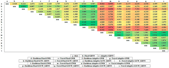
Figure 6.
Statistical results of McNemar’s Test.
Supposing the similarity of the kernel, in the case of ED or TD, the amount of |Z| resulting from McNemar’s Test is less than 2.575 in all GWR, GCW-GRNN, GTWR, and GTCW-GRNN algorithms. Therefore, replacing TD with ED with a 99% confidence level does not make a significant difference.
Considering the negation signs in Figure 6, GTWR has better performance compared to OLS and GWR models. The amount of Z in threshold 1% for GTWR against OLS and GWR (in ED, TD, fixed kernel, and adaptive kernel) is always less than −2.575 in all states. Thus, the GTWR model has significantly higher accuracy than the GWR and OLS models. The results show a significant difference between GTWR against GWR and OLS at a 99% confidence level. The performance of the developed GRNN models (fixed and adaptive) will be examined separately.
Considering the negation signs in Figure 6, fixed GTCW-GRNN has better performance compared to fixed GRNN and fixed GCW-GRNN models. The amount of Z in threshold 0.1% for fixed GTCW-GRNN against fixed GRNN and fixed GCW-GRNN, using ED or TD, is less than −2.575. Therefore, fixed GTCW-GRNN model has significantly higher accuracy compared to the fixed GRNN and fixed GCW-GRNN models. The results show a significant difference between the fixed GTCW-GRNN against fixed GRNN and fixed GCW-GRNN in a 99% confidence level.
Finally, considering the negation signs in Figure 6, adaptive GTCW-GRNN has better performance than the adaptive GRNN and adaptive GCW-GRNN models. The amount of Z in threshold 1% for adaptive GTCW-GRNN against adaptive GRNN and adaptive GCW-GRNN, using ED or TD, is less than −2.575. Therefore, adaptive GTCW-GRNN model has a significantly higher accuracy than adaptive GRNN and adaptive GCW-GRNN models. The results show a significant difference between adaptive GTCW-GRNN against Adaptive GRNN and Adaptive GCW-GRNN in a 99% confidence level.
7. Discussion
Compared to the GRNN model, the mean R-Squared index value in the GCW-GRNN model decreased by 0.001; however, the mean R-Squared index value in the GTCW-GRNN model increased by 0.037. Furthermore, it improved in the GWR and GTWR models by 0.035 and 0.083, respectively, compared to the OLS model. Therefore, the GWR and GTWR models have more power in expressing the spatial distribution and spatiotemporal distribution, respectively, compared to the GCW-GRNN and GTCW-GRNN models.
As the GRNN model captures the non-linear relationship between the dependent and independent variables, the GRNN model is therefore more accurate than the OLS model. The R-Squared and RMSE statistical indicators confirm this statement. Considering the high power of the GWR and GTWR models in expressing spatial and spatiotemporal distributions, they have more accuracy than the GCW-GRNN and GTCW-GRNN models.
The GTWR model has two components of location and time. The GTCW-GRNN model has a feature component in addition to the location and time components. Therefore, the probability of the assigned weight to the y of each training point reaching zero, in the case of the adaptive kernel, is higher in the GTCW-GRNN model compared to the GTWR model. Therefore, in the case of the adaptive kernel, the average of the R-Squares indicator in the GTCW-GRNN model is 0.028 less than in the GTWR model. GWR has one less parameter than the GCW-GRNN model with only the location parameter. Accordingly, when the adaptive kernel is applied, the mean R-Squared index in the GCW-GRNN model is 0.025 lower than in the GWR model.
As the observation points are dense, the fixed kernel always has a better performance compared to the adaptive kernel. Using a fixed kernel in GRNN, GWR, GCW-GRNN, GTWR, and GTCW-GRNN models improved the average of the R-Squared indicator by 0.008, 0.003, 0.010, 0.012, and 0.006, respectively. Using a fixed kernel, therefore, always results in higher R-Squared and lower RMSE. The GRNN is faster than OLS. OLS has no parameter to be set during the training process, while the bandwidth of the physical features has to be determined for the GRNN model and, therefore, training the GRNN is slower. GCW-GRNN and GTCW-GRNN have one parameter more than the GWR and GTWR models. But considering the high speed of the GCW-GRNN and GTCW-GRNN models, their training takes less time compared to GWR and GTWR. Using TD instead of ED, generally, makes the value of |Z| resulting from McNemar’s Test less than 2.575 at a 99% confidence level. The biggest difference occurs in comparing Travel Fixed GTCW-GRNN and Euclidean Fixed GTCW-GRNN models, for which the value of |Z|, in this case, equals 1.732. Therefore, using TD instead of ED does not make a significant difference at the 99% confidence level.
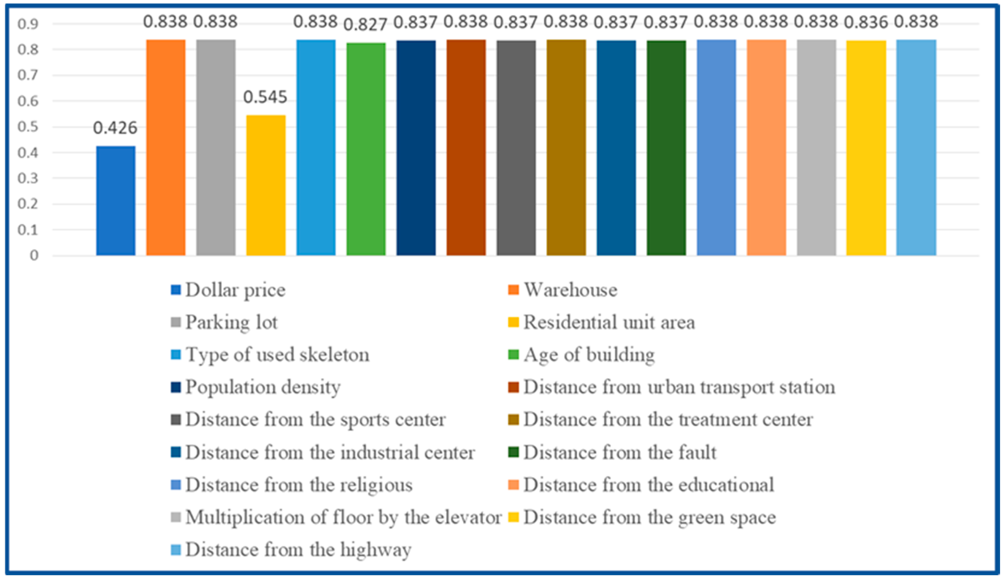
The technique with the best results is the GTWR method with a fixed kernel and Euclidean distance. As a consequence, each independent variable was eliminated independently to examine the sensitivity of each independent variable to the dependent variable, which is the housing price. The Euclidean Fixed GTWR model was then applied to the remaining variables, with the findings shown in Figure 7. Figure 7 shows that the adjusted coefficient of determination from the Euclidean Fixed GTWR method will be equivalent to 0.425 if the exchange rate variable (dollar price) is removed from the independent variables to model the housing price. The exchange rate variable will thus have the most effect on house price modeling. The area of the residential unit has the most influence on housing price modeling after the exchange rate variable. The modified determination coefficient will equal 0.544 if the residential unit area variable is removed from the independent variables in the housing price modeling. The variables of building age, distance from a sports center, distance from green space, distance from the industrial center, distance from a fault, population density, and distance from a medical center have a greater impact on the housing price modeling at the 95% confidence level as well.
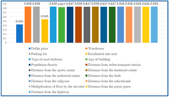
Figure 7.
The adjusted coefficient of determination value according to the elimination of each variable in housing price modeling.
The summary of the data indicates that the exchange rate and other external and economic factors can have the most effects on housing price modeling. The physical qualities of the house, such as the area of the residential unit and the age of the building, have a major impact on the modeling of housing price after the exchange rate variable. The results of housing price modeling can be improved by including additional variables like the property’s level of safety, such as the distance from a fault, and the level of access to urban services, such as the distance from medical, sporting, educational, and religious centers, distance from green space, distance from the highway, and distance from urban transportation stations.
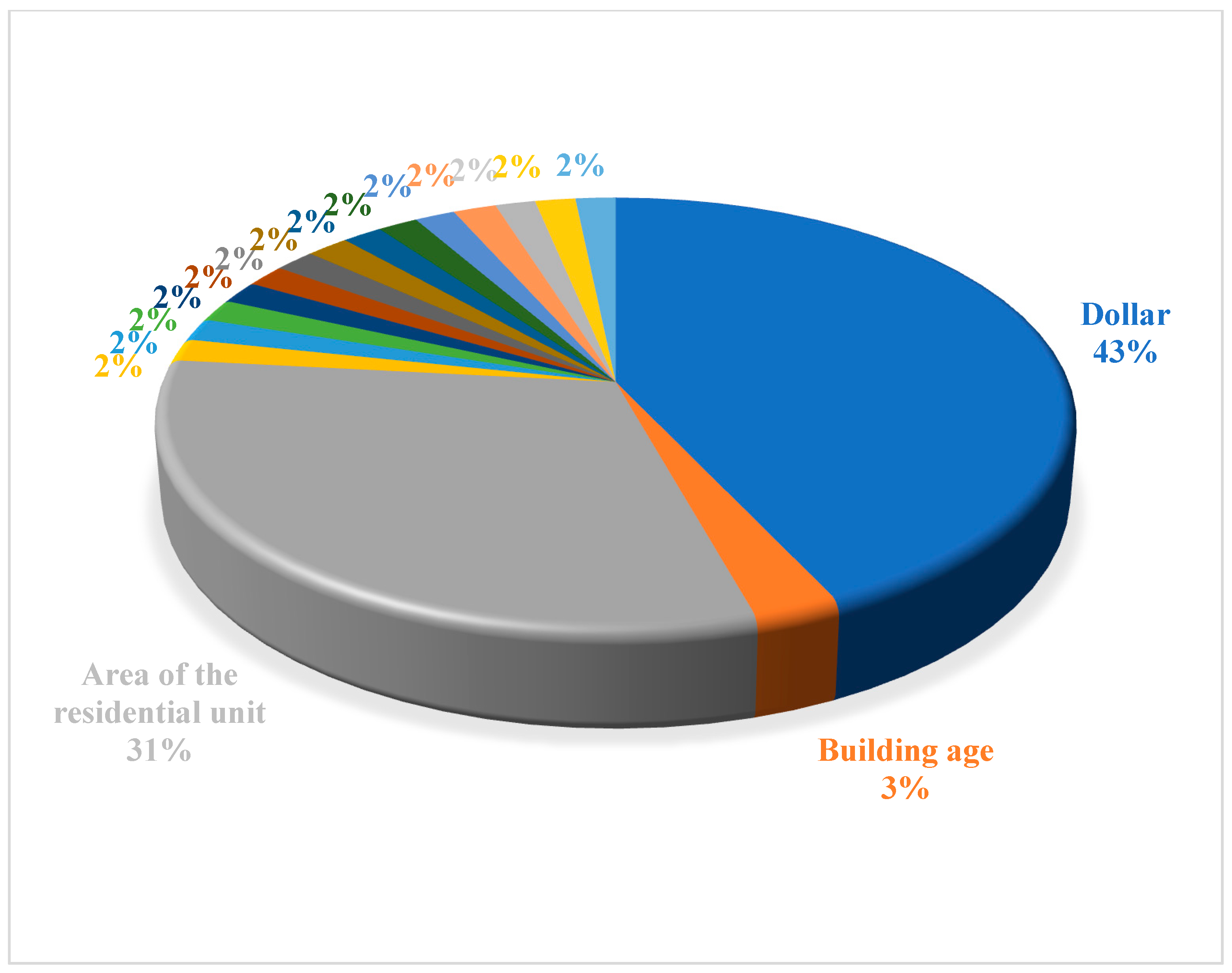
In order to understand how much each variable is influential in the Euclidean Fixed GTWR model, this study summarizes the results of Figure 7 in Figure 8 and shows the effectiveness of each variable as a percentage. In order to make Figure 8 less crowded, this study only shows the names of the three most influential variables, i.e., the dollar, area, and building age variables. The rest of the variables are influential in modeling the Euclidean Fixed GTWR method by 2%.

Figure 8.
The influence of each variable in the modeling of the Euclidean Fixed GTWR method.
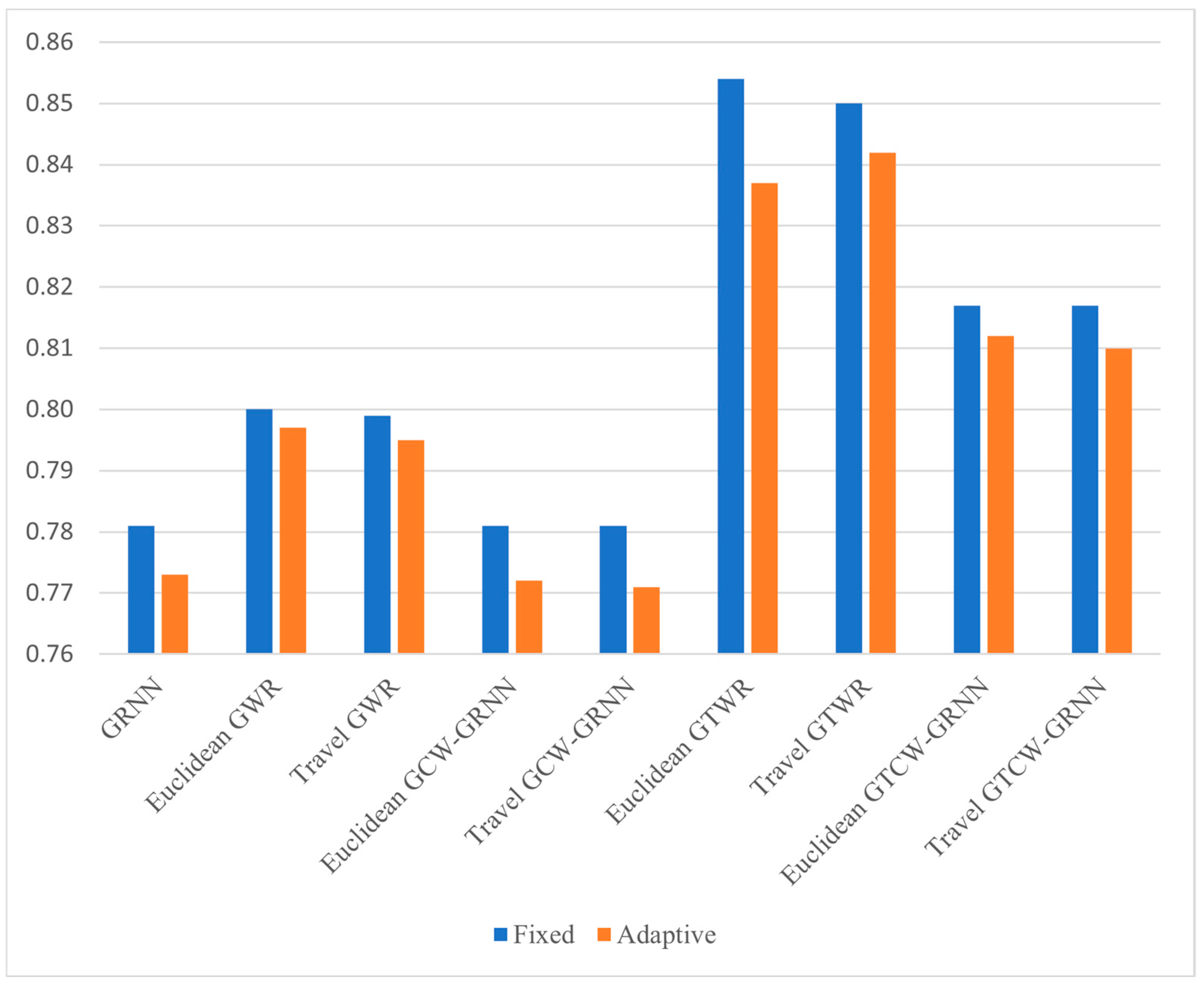
In order to compare the adjusted coefficient of determination in different fixed and adaptive modes, Figure 9 was prepared. Figure 9 is a summary of Figure 4 for different fixed and adaptive modes in the investigated models. As it is clear in this figure, in all models, the fixed mode is more accurate than the adaptive mode.
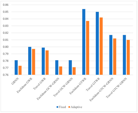
Figure 9.
Adjusted coefficient value in different models in different fixed and adaptive modes.
According to Figure 4 and based on RMSE and Adjusted R-Squared indicators, it can be said that in both fixed and adaptive modes, the GRNN model performs better than the OLS model, indicating the presence of a non-linear relationship in the independent variables that the OLS model cannot model. The GCW-GRNN model performs worse than the GWR model, implying that a linear relationship in the spatial dimension between the independent variables causes the GWR model to outperform the GCW-GRNN. Furthermore, the GTCW-GRNN model performs worse than the GTWR model, indicating that the independent variables have a linear relationship in the spatiotemporal dimensions.
In each of the fixed and adaptive modes in the GRNN model and its derivatives, according to Figure 4 and Figure 6, it can be concluded that considering the spatial, temporal, and characteristic parameters leads to an improvement in results. Therefore, according to the obtained results, the GTCW-GRNN model is more accurate in comparison with the GCW-GRNN and GRNN models.
8. Conclusions
The GRNN algorithm developed in this research effectively models the spatial and spatiotemporal heterogeneity in housing price data, considering both physical housing features and other factors. Therefore, the GCW-GRNN and GTCW-GRNN models are presented based on the GRNN algorithm. One of the advantages of the GRNN algorithm is its high power in modeling non-linear relations among dependent and independent variables. As the results demonstrate, GRNN achieves higher accuracy than the OLS model due to the latter feature.
In this research, all variables were assigned a single bandwidth. As there were three bandwidths, it was proposed to develop GCW-GRNN and GTCW-GRNN algorithms to provide Multiscale GCW-GRNN and Multiscale GTCW-GRNN models, and to compare the results of Multiscale GWR and Multiscale GTWR for future works. To maximize the impact of this research, we suggest developing the proposed GTCW-GRNN model into an optimized software library for broader adoption. The open-source implementation currently available on GitHub (https://github.com/SaeidZali/GTCW-GRNN accessed on 22 April 2024) provides a valuable starting point for such library development.
Author Contributions
Conceptualization, S.Z. and P.P.; Methodology, S.Z. and O.G.; Software, S.G.; Validation, M.A.; Formal analysis, A.K.; Investigation, S.G.; Data curation, P.P.; Writing—original draft, S.Z.; Writing—review & editing, P.P. and O.G.; Visualization, O.G.; Supervision, P.P. and O.G. All authors have read and agreed to the published version of the manuscript.
Funding
This research received no external funding.
Data Availability Statement
The raw data supporting the conclusions of this article will be made available by the authors on request.
Acknowledgments
We appreciate the support provided by the University of Natural Resources and Life Sciences Vienna (BOKU).
Conflicts of Interest
The authors declare no conflicts of interest.
References
- Tobler, W.R. A computer movie simulating urban growth in the Detroit region. Econ. Geogr. 1970, 46, 234–240. [Google Scholar] [CrossRef]
- Baltagi, B.H. A Companion to Theoretical Econometrics; Wiley Online Library: Hoboken, NJ, USA, 2001; Volume 1. [Google Scholar]
- Belke, A.; Keil, J. Fundamental determinants of real estate prices: A panel study of German regions. Int. Adv. Econ. Res. 2017, 24, 25–45. [Google Scholar] [CrossRef]
- Chen, Y.; Wu, S.; Wang, Y.; Zhang, F.; Liu, R.; Du, Z. Satellite-Based Mapping of High-Resolution Ground-Level PM2.5 with VIIRS IP AOD in China through Spatially Neural Network Weighted Regression. Remote Sens. 2021, 13, 1979. [Google Scholar] [CrossRef]
- Martinez-Blanco, M.d.R.; Ornelas-Vargas, G.; Solis-Sánchez, L.O.; Castañeda-Miranada, R.; Vega-Carrillo, H.R.; Celaya-Padilla, J.M.; Garza-Veloz, I.; Martinez-Fierro, M.; Ortiz-Rodriguez, J.M. A comparison of back propagation and generalized regression neural networks performance in neutron spectrometry. Appl. Radiat. Isot. 2016, 117, 20–26. [Google Scholar] [CrossRef]
- Wu, C.; Ren, F.; Hu, W.; Du, Q.; Wu, C. Multiscale geographically and temporally weighted regression: Exploring the spatio-temporal determinants of housing prices. Int. J. Geogr. Inf. Sci. 2019, 33, 489–511. [Google Scholar] [CrossRef]
- Li, T.; Shen, H.; Yuan, Q.; Zhang, L. Geographically and temporally weighted neural networks for satellite-based mapping of ground-level PM2.5. ISPRS J. Photogramm. Remote Sens. 2020, 167, 178–188. [Google Scholar] [CrossRef]
- Casetti, E. Generating models by the expansion method: Applications to geographical research. Geogr. Anal. 1972, 4, 81–91. [Google Scholar] [CrossRef]
- Geerts, M.; vanden Broucke, S.; De Weerdt, J. A Survey of Methods and Input Data Types for House Price Prediction. ISPRS Int. J. Geo-Inf. 2023, 12, 200. [Google Scholar] [CrossRef]
- Fu, R.; Huang, Z.; Lin, Y.; Tang, X.; Zheng, Z.; Hu, Z. Temporal-spatial distribution characteristics and associated socioeconomic factors of visiting frequency for rural patients with hypertension in Fujian Province, Southeast China. BMC Public Health 2024, 24, 656. [Google Scholar] [CrossRef]
- Brunsdon, C.; Fotheringham, A.S.; Charlton, M. Some notes on parametric significance tests for geographically weighted re-gression. J. Reg. Sci. 1999, 39, 497–524. [Google Scholar] [CrossRef]
- Bełej, M.; Cellmer, R.; Foryś, I.; Głuszak, M. Airports in the urban landscape: Externalities, stigmatization and housing market. Land Use Policy 2023, 126, 106540. [Google Scholar] [CrossRef]
- Fotheringham, A.S.; Yang, W.; Kang, W. Multiscale geographically weighted regression (MGWR). Ann. Am. Assoc. Geogr. 2017, 107, 1247–1265. [Google Scholar] [CrossRef]
- He, J.; Shi, Y.; Xu, L.; Lu, Z.; Feng, M. An investigation on the impact of blue and green spatial pattern alterations on the urban thermal environment: A case study of Shanghai. Ecol. Indic. 2024, 158, 111244. [Google Scholar] [CrossRef]
- Lu, B.; Charlton, M.; Harris, P.; Fotheringham, A.S. Geographically weighted regression with a non-Euclidean distance metric: A case study using hedonic house price data. Int. J. Geogr. Inf. Sci. 2014, 28, 660–681. [Google Scholar] [CrossRef]
- Vichiensan, V.; Wasuntarasook, V.; Prakayaphun, T.; Kii, M.; Hayashi, Y. Influence of Urban Railway Network Centrality on Residential Property Values in Bangkok. Sustainability 2023, 15, 16013. [Google Scholar] [CrossRef]
- Huang, B.; Wu, B.; Barry, M. Geographically and temporally weighted regression for modeling spatio-temporal variation in house prices. Int. J. Geogr. Inf. Sci. 2010, 24, 383–401. [Google Scholar] [CrossRef]
- Xiao, F.; Wang, J.; Xiong, M.; Mo, H. Does spatiotemporal heterogeneity matter? Air transport and the rise of high-tech industry in China. Appl. Geogr. 2024, 162, 103148. [Google Scholar] [CrossRef]
- Liu, J.P.; Yang, Y.; Xu, S.H.; Zhao, Y.Y.; Wang, Y.; Zhang, F.H. A geographically temporal weighted regression approach with travel distance for house price estimation. Entropy 2016, 18, 303. [Google Scholar] [CrossRef]
- Chica-Olmo, J.; Cano-Guervos, R.; Chica-Rivas, M. Estimation of Housing Price Variations Using Spatio-Temporal Data. Sustainability 2019, 11, 1551. [Google Scholar] [CrossRef]
- Liu, T.; Wang, J.; Liu, L.; Peng, Z.; Wu, H. What Are the Pivotal Factors Influencing Housing Prices? A Spatiotemporal Dynamic Analysis Across Market Cycles from Upturn to Downturn in Wuhan. Land 2025, 14, 356. [Google Scholar] [CrossRef]
- Chang, Y.-M.; Wang, Y.-T. A Spatial–Temporal Model of House Prices in Northern Taiwan. Mathematics 2025, 13, 736. [Google Scholar] [CrossRef]
- Jiang, R.; Wang, H.; Huang, B.; Guo, G. An Improved Geographically and Temporally Weighted Regression Model with a Novel Weight Matrix. In Proceedings of the 12th International Conference on Geo-Computation, Wuhan, China, 23–25 May 2013. [Google Scholar]
- Bidanset, P.; McCord, M.; Lombard, J.A.; Davis, P.; McCluskey, W. Accounting for locational, temporal, and physical similarity of residential sales in mass appraisal modeling: The development and application of geographically, temporally, and characteris-tically weighted regression. J. Prop. Tax Assess. Adm. 2018, 14, 5–13. [Google Scholar] [CrossRef]
- Yousfi, S.; Dubé, J.; Legros, D.; Thanos, S. Mass appraisal without statistical estimation: A simplified comparable sales approach based on a spatiotemporal matrix. Ann. Reg. Sci. 2020, 64, 349–365. [Google Scholar] [CrossRef]
- Zeng, X.; Chen, Y.W.; Tao, C. Feature selection using recursive feature elimination for handwritten digit recognition. In Proceedings of the 2009 5th International Conference on Intelligent Information Hiding and Multimedia Signal Processing, Kyoto, Japan, 12–14 September 2009. [Google Scholar]
- Specht, D.F. A general regression neural network. IEEE Trans. Neural Netw. 1991, 2, 568–576. [Google Scholar] [CrossRef] [PubMed]
- Yahya, S.I.; Rezaei, A.; Aghel, B. Forecasting of water thermal conductivity enhancement by adding nano-sized alumina particles. J. Therm. Anal. Calorim. 2021, 145, 1791–1800. [Google Scholar] [CrossRef]
- Zhang, S.; Lei, L.; Sheng, M.; Song, H.; Li, L.; Guo, K.; Ma, C.; Liu, L.; Zeng, Z. Evaluating Anthropogenic CO2 Bottom-Up Emission Inventories Using Satellite Observations from GOSAT and OCO-2. Remote Sens. 2022, 14, 5024. [Google Scholar] [CrossRef]
- Li, C.F.; Zhang, J.B.; Wang, S.T. Comparative study on input-expansion-based improved general regression neural network and Levenberg-Marquardt BP network. In Intelligent Computing, Proceedings of the International Conference on Intelligent Computing, Kunming, China, 16–19 August 2006; Springer: Hoboken, NJ, USA, 2006. [Google Scholar]
- Shao, Z.; Wang, Y.; Chen, X. Global prescribed performance control for strict feedback systems pursuing uncertain target. IEEE Trans. Neural Netw. Learn. Syst. 2022, 35, 2403–2412. [Google Scholar] [CrossRef]
- Pai, P.F.; Wang, W.C. Using machine learning models and actual transaction data for predicting real estate prices. Appl. Sci. 2020, 10, 5832. [Google Scholar] [CrossRef]
- Oshan, T.M.; Li, Z.; Kang, W.; Wolf, L.J.; Fotheringham, A.S. mgwr: A Python implementation of multiscale geographically weighted regression for investigating process spatial heterogeneity and scale. ISPRS Int. J. Geo-Inf. 2019, 8, 269. [Google Scholar] [CrossRef]
- Foody, G.M. Thematic map comparison. Photogramm. Eng. Remote Sens. 2004, 70, 627–633. [Google Scholar] [CrossRef]
- Debnath, M.; Islam, N.; Gayen, S.; Roy, P.; Sarkar, B.; Ray, S. Prediction of spatio-temporal (2030 and 2050) land-use and land-cover changes in Koch Bihar urban agglomeration (West Bengal), India, using artificial neural network-based Markov chain model. Model. Earth Syst. Environ. 2023, 9, 3621–3642. [Google Scholar] [CrossRef]
- Bahmani-Oskooee, M.; Wu, T.P. Housing prices and real effective exchange rates in 18 OECD countries: A bootstrap multivariate panel Granger causality. Econ. Anal. Policy 2018, 60, 119–126. [Google Scholar] [CrossRef]
- Salisu, A.; Rufai, A.; Chidi, M. Exchange rate and housing affordability in OECD countries. Int. J. Hous. Mark. Anal. 2024, 18, 668–693. [Google Scholar] [CrossRef]
- Soltani, A.; Heydari, M.; Aghaei, F.; Pettit, C.J. Housing price prediction incorporating spatio-temporal dependency into machine learning algorithms. Cities 2022, 131, 103941. [Google Scholar] [CrossRef]
- Mehmani, A.; Chowdhury, S.; Messac, A. Predictive quantification of surrogate model fidelity based on modal variations with sample density. Struct. Multidiscip. Optim. 2015, 52, 353–373. [Google Scholar] [CrossRef]
- Kiefer, J. Sequential minimax search for a maximum. Proc. Am. Math. Soc. 1953, 4, 502–506. [Google Scholar] [CrossRef]
- Deb, K. Optimization for Engineering Design: Algorithms and Examples; Prentice Hall: New Delhi, India, 1995. [Google Scholar]
- Chakraborty, S.K.; Panda, G. Golden Section Search over a hyper-rectangle: A direct search method. Int. J. Math. Oper. Res. 2016, 8, 279–292. [Google Scholar] [CrossRef]
- Rani, G.S.; Jayan, S.; Nagaraja, K.V. An extension of golden section algorithm for n-variable functions with MATLAB code. In IOP Conference Series: Materials Science and Engineering, Proceedings of the International Conference on Advances in Materials and Manufacturing Applications (IConAMMA-2018), Bengaluru, India, 16–18 August 2018; IOP Publishing Ltd.: Bristol, UK, 2018; Volume 577, p. 012175. [Google Scholar]
- Adebayo, I.G.; Abdulrahaman, O.K.; Olaniyan, O.M.; Adeyanju, I.A.; Ogunbiyi, O. Multi-Objective Golden Flower Optimization Algorithm for Sustainable Reconfiguration of Power Distribution Network with Decentralized Generation. Eng. Proc. 2023, 29, 13. [Google Scholar]
- Powell, M.J.D. An efficient method for finding the minimum of a function of several variables without calculating derivatives. Comput. J. 1964, 7, 155–162. [Google Scholar] [CrossRef]


Disclaimer/Publisher’s Note: The statements, opinions and data contained in all publications are solely those of the individual author(s) and contributor(s) and not of MDPI and/or the editor(s). MDPI and/or the editor(s) disclaim responsibility for any injury to people or property resulting from any ideas, methods, instructions or products referred to in the content. |
© 2025 by the authors. Licensee MDPI, Basel, Switzerland. This article is an open access article distributed under the terms and conditions of the Creative Commons Attribution (CC BY) license (https://creativecommons.org/licenses/by/4.0/).