Investigating the Nonlinear Relationship Between the Built Environment and Urban Vitality Based on Multi-Source Data and Interpretable Machine Learning

Abstract

Optimizing the built environment to foster urban vitality is essential for effective urban planning and sustainable development. Previous studies have predominantly focused on analyzing the relationship between the built environment and urban vitality at either a macro or micro-scale, often assuming a predefined linear relationship. In this study, we investigate the potential non-linear interactions between the built environment and urban vitality by employing an interpretable spatial machine learning framework that integrates the XGBoost model with the SHapley Additive exPlanations (SHAP) algorithm. Additionally, we analyze the determinants of urban vitality across both micro and macro-scales using multi-source data, semantic segmentation models, and street view imagery. Our findings reveal the following key insights: (1) the distribution of urban vitality exhibits spatial heterogeneity within the main urban area of Shanghai, with high vitality areas concentrated in the Huangpu District and at intersections with neighboring districts, demonstrating a decline from the center to the periphery; (2) the XGBoost model outperforms other comparative models, showcasing superior capabilities in simulating and predicting urban vitality; (3) among the various built environment factors influencing urban vitality, building coverage, population density, and distance to the CBD exert the most significant effects, while the green view index and the number of bus stops contribute relatively less; (4) all built environment factors demonstrate nonlinear impacts and exhibit certain threshold effects on urban vitality. The analytical outcomes of this study provide valuable insights for optimizing the spatial layout and resource allocation within urban settings, offering references for urban planning and sustainable development initiatives.

1. Introduction

The concept of urban vitality, which symbolizes the exuberance of a city, was first proposed by Jane Jacobs, who argued that a certain density of people in a city represents a wealth of unparalleled differences and possibilities. The dynamic interplay between these human activities and the environment brings vitality and diversity to the city [1]. Urban vitality is the basis of urban evolution and the propulsion of urban development. Many researchers have investigated urban vitality through various perspectives. They see that urban vitality is an interaction of diverse residential activities and complex environments influenced by the spatial pattern of the city [2,3]. As the economic center and international metropolis of China, the diversity of the built environment and spatial structure of the city of Shanghai is one of the important issues facing urban planning and management. With advancement of urbanization in China, Shanghai’s built environment pattern has changed significantly. The spatial distribution and utilization of the built environment have shown complex evolutionary characteristics, which has resulted in numerous urban issues, resulting in the decline of urban vitality, potentially hindering the sustainable development of the city. Urban vitality reflects the complex interaction of social, economic, and cultural factors, which directly affects the attractiveness of the city and the happiness index of its residents [4]. Therefore, it is a scientific problem to be solved in urban spatial planning and design to study the influence of built environment on urban vitality and optimize the built environment so as to stimulate urban vitality. Analyzing the association between the built environment and urban vitality in Shanghai from both a more detailed micro perspective and a macro overall perspective holds substantial implications for urban planning and sustainable development.

Traditional urban vitality research is mainly based on survey data or interviews [2,5,6], which, having high time and manpower costs, cannot be implemented on a large scale, making it difficult to provide guiding opinions for urban planning. In recent years, a new data environment containing big data and open data has been gradually forming, and the assessment of urban vitality has evolved to encompass a broader range of indicators and greater precision. Currently, diverse large-scale datasets are widely used to carry out research concerning the built environment and urban vitality [7,8,9,10]. Point of interest (POI) data, building vector data, road network, metro station, etc., provide the possibility of extracting built environment elements such as functional mixing, density, and traffic. This can realize comprehensive spatial statistics across city dimensions and macroscopically understand the interaction mechanism between environmental elements and urban vitality. However, despite irreplaceable advantages of macro-scale analyses in revealing large-scale urban development trends, there are still limitations in portraying urban details, especially street-level spatial characteristics. High-precision information at the street level, such as the canopy width of trees, the width of street green belts, and the space for pedestrian activities, are details that are significant for assessing the livability of the urban living environment and the accessibility of the transport environment. Traditional macro-scale analyses have difficulty identifying building façade features, pavement details, street furniture, and vegetation shading in the streetscape, which are important in improving the daily living standards of city dwellers and urban environment quality. In this context, some studies have begun to try to combine street-view-image data with semantic segmentation techniques [11,12,13] to analyze the spatial configuration of metropolitan streets at micro-scale viewpoint. For example, through the semantic segmentation of street view imagery, it is possible to accurately identify different elements within the visual scene (e.g., buildings, trees, roads, and pavements) and calculate indicators reflecting the level of street greening, such as green visibility. This provides new perspectives and methods for analyzing urban environments at the micro-level.

Simultaneously, Shanghai, as a mega-city in China and even globally, has a complex and diverse urban structure, with significant differences in road network density, population density, and land-use diversity between different regions. For example, central urban areas tend to have higher population and road network densities, while suburban areas may exhibit lower development intensity and higher green coverage. The diversity of land use types in different areas also reflects the differentiated characteristics of Shanghai in terms of functional zoning. How to integrate these diverse spatial features at the macro-scale and combine them with the streetscape features at the micro-scale, so as to systematically reveal the driving factors behind the urban vitality features and built environment of Shanghai, has become a difficult and challenging task in the current research field.

Built environment generally refers to the human-made environment that has been planned and transformed. We refer to the “5Ds” built environment indicator system (density, diversity, design, destination accessibility, and distance to transit) proposed by Ewing et al. [14]. We synthesize the constructed indicator system [11,15,16] and select the corresponding indicators as macro variables based on the availability of data and the appropriateness of indicators. Since this paper focuses on research at two scales and highlights the importance of urban environmental factors at the micro-level, we divide the indicators into macro variables and micro variables.

In the studies on built environment and urban vitality, Lyu et al. [17] combined linear regression and geographically weighted regression to analyze the effect of built environment on urban vitality. The results of the study showed that built environment factors significantly affect urban vitality and display spatial heterogeneity in different regions. Zhang et al. [10] proposed a system consisting of three dimensions (urban form, urban village, and urban function) by integrating built environment factors of a city and used a spatial lag model to explain the impact of the built environment on vitality. It was found that dense road networks, abundant transportation, and commercial facilities are positive factors affecting urban vitality, while urban villages and residential compounds have a negative impact on urban vitality. Yang et al. [15] employed gradient boosting decision trees to investigate the nonlinear association between the built environment and urban vitality using Shenzhen as a case study. The results show that the total floor area and access to destinations are the key factors affecting urban vitality, while most built environment variables have respective upper thresholds. Ma et al. [11] explored the street characteristics of the city in depth using relevant data from Qingdao. They extracted relevant indicators in street view images as visual perception factors and analyzed the drivers of urban vitality using random forest and SHAP methods.

Considering the bias of linear assumption, the recent literature has utilized different machine learning methods for nonlinear analysis of other behaviors related to the built environment [18,19,20,21,22]. For example, Gao et al. [19] identified key built environment features that influence cycling volume by using crowdsourced tracker data and machine learning and found that proximity to blue space is the most important factor in promoting cycling volume. In addition, they utilized partial dependence plots to elucidate the nonlinear relationships between environmental features and cycling volume, revealing its nonlinear and threshold effects on cycling. Yang et al. [20] explored the nonlinear and synergistic effects of green spaces on two types of active travel (cycling and running) by analyzing survey data in Chengdu using random forest and SHAP methods and derived the importance ranking of different features on the model prediction results through feature importance analysis. The findings suggest that green spaces can account for up to 20% of the variance in active travel. In addition, some works extracted relevant elements from street view images for research. For example, Liu et al. [21] explored the nonlinear effects of built environment on jogging behavior using random forest, while they used semantic segmentation to extract environmental elements from street view images as independent variables and found that built environment factors have different nonlinear effects on jogging at trip and origin-destination (OD) levels. In another example, Chen et al. [13] used semantic segmentation to extract the green view index from street view images as a dependent variable to study the nonlinear effects of environmental features on green view index. Machine learning has proven to be advantageous in capturing these complex nonlinear relationships, providing greater insight into the effects of variables that are not easily identified through traditional linear models. In contrast, fewer studies have explored the nonlinear effects of the built environment on urban vitality. In this sense, the nonlinear effects of the built environment on urban vitality warrant further attention.

In summary, this literature review suggests that less attention has been given to nonlinear aspect in studies on the built environment and urban vitality, and less attention has been given to urban vitality in nonlinear studies of the built environment and public behavior. Meanwhile, previous studies have employed linear regression frameworks, spatial econometric methodologies, and geographically weighted regression models [23,24,25,26,27] to investigate the influence and significance of environmental elements on vitality. To a certain degree, some research demonstrated that certain environmental elements are correlated with urban vitality, offering valuable implications for spatial planning strategies. Nevertheless, current research has several deficiencies. On the one hand, these studies usually suppose that the built environment and urban vitality follow a predefined linear relationship and ignore the nonlinear relationship [10,17,28,29]. This may underestimate the correlation between urban vitality and the built environment variables, which may lead to misguided impacts on urban planning and management. On the other hand, most of the current research analyzes the impact of the built environment on urban vitality from a single macro or micro-scale [15,26,30] and seldom explores the differences in the impact mechanism between them from both micro and macro-scales. This paper aims to bridge these gaps.

In addition, existing research lacks an explanation of model localization; this phenomenon results in the mechanisms of its operation becoming opaque, making it difficult to analyze its influencing factors in depth [20]. SHapley Additive exPlanations (SHAP) and Local Interpretable Model-agnostic Explanations (LIME) are both common interpretable machine learning methods, each with its own characteristics. In this study, we use the SHAP method to visualize the results and improve the transparency and readability of the models [13,20,31]. SHAP relies on the Shapley value in game theory and is able to provide a consistent and fair assessment of the contribution of each feature, which makes the interpretation of feature importance more theoretically grounded and reliable. Additionally, SHAP provides both global and local interpretability, offering a more comprehensive view for understanding the overall behavior of the model as well as specific predictions. In addition, the consistency property of SHAP implies that when the model is adjusted or the importance of features changes, the corresponding interpreted results will change accordingly, which enhances the credibility of the model results. In contrast, LIME’s local model generation process, although flexible, may lead to instability and randomness in result interpretation. Therefore, based on the above considerations, the SHAP method is more suitable for the needs of this study.

To bridge the gaps mentioned above, in this study, using data from Shanghai, China, we combine the XGBoost model with the SHAP method to investigate complex nonlinear interactions between the built environment and urban vitality. Starting from both micro and macro-scales, we apply the semantic segmentation technique to street view imagery to extract micro factors such as green view index and openness ratio at the street level, characterizing the environmental quality of different areas. At the same time, urban vitality in Shanghai is systematically analyzed using macro-scale elements such as road network density, population density, and land-use entropy, aiming to reveal the spatial differences in urban vitality across various regions and their influencing factors. Through a comprehensive analysis of these multi-dimensional data, this research expects to establish an evidence-based framework for future urban development strategies and spatial optimization in Shanghai and also serve as a reference for research in other metropolises. The remainder of the paper is organized as follows. Section 2 describes the study area and data. Section 3 describes the research methodology. Section 4 describes the analysis of results. Section 5 discusses the results and presents limitations and future work. The final section presents key findings.

2. Study Area and Data

2.1. Study Area

Situated on China’s eastern coast, Shanghai is a significant national economic, financial, trade, and shipping center, as well as a globally renowned mega-city. In the study, Shanghai’ main urban region is designated as this study area, as shown in Figure 1. As a representative area of China’s urbanization process, the main urban area of Shanghai holds important research value with regard to land use, urban spatial structure, and population agglomeration. The central urban zone is situated in the heart of Shanghai, encompassing the districts of Huangpu, Xuhui, Changning, Jing’an, Putuo, Hongkou, and Yangpu and covering the core sites on both sides of the Huangpu River, including both the early developed traditional urban areas and the emerged modernized areas in recent years. This choice of scope enables the study to investigate the built environment’s characteristics and the progression of spatial structure in Shanghai at different stages of development, providing a rich sample for a multi-dimensional study of associations between urban vitality and the environmental elements.

In this study, the main urban area of Shanghai is divided into 1764 cells using a 500 m × 500 m square grid in the spatial dimension [10,15]. The variables are measured at the grid level to ensure that the cell division better matches the spatial scale of the neighborhoods in the central urban area. This approach aims to achieve the research goal of the spatio-temporal visualization of urban vitality and its relationship with the built environment at the neighborhood scale.

2.2. Data Source

Multiple sources of data were used in the research, including the Baidu Heat Index from Baidu Heat Map, street view photos from Baidu Street View Map, data on land-use entropy derived from points of interest (POIs) provided by Baidu Map, data on road network density and intersection density from OpenStreetMap (OSM), data on population density from the WorldPop database, and data on the distance to CBD, as well as the number of metro and bus stops derived from AMap.

2.3. Measurement of Urban Vitality (Dependent Variable)

Urban vitality is defined as active communication activities that take place in an urban space at various times of the day [32]. These activities are measured by people’s visits to the space during different periods. The more intensive the activity, the more vibrant the space and the city become. Therefore, we chose urban vitality as the dependent variable, which is characterized by Baidu Heat Map data. People’s visits can be recorded by the app. The location information of users using Baidu Maps and other Baidu mobile apps that provide location services is recorded 24/7 at one-hour intervals. This user location information is then projected onto the space to calculate the Baidu Heat Index, reflecting the spatial distribution of the users using various colors. Baidu Heat Map data provide an extensive coverage of the population, with the advantages of real-time dynamic updates, fine granularity, and high precision. These kinds of data, which can objectively and realistically reflect the dynamic changes in crowd activity density, have been widely used as a metric for assessing urban vitality [15,17,33].

In this study, we collected Baidu Heat Map data of Shanghai for five weekdays from June 3rd to June 7th, 2024, and used the average value of the collected Baidu Heat Index to characterize the urban vitality of each spatial unit. Figure 2 shows the spatial distribution characteristics of vitality in Shanghai’s main urban area. In general, the high-value areas of vitality are distributed in the center of the study area (Huangpu District and the intersections with other districts to the west of Huangpu District), and the vitality exhibits a radial decay pattern emanating from central zones towards peripheral areas.

2.4. Built Environment Elements (Independent Variables)

The independent variables data in this study include both micro and macro-levels to explore the influences of environmental elements on urban vitality from these two scales. Relevant descriptive and statistical results for all variables are shown in

Table 1. Variable definitions and descriptive statistics.

Variables	Variable Description	Mean	S.D.	Min	Max
Urban vitality	Average Baidu Heat Index	318.44	250.51	0	2419
Micro variables
Road coverage rate	Proportion of pixels occupied by roads in street view images	10.11%	2.91%	1.93%	43.82%
Building coverage rate	Proportion of pixels occupied by buildings in street view images	19.01%	10.56%	0.04%	74.02%
Green view index	Proportion of pixels occupied by green vegetation (e.g., trees, grass, shrubs, etc.) in street view images	22.94%	13.16%	0	78.13%
Openness ratio	Proportion of pixels occupied by sky in street view images	37.35%	12.87%	0.02	73.49%
Macro variables
Population density	Number of people in the region/area of the region (person/km2)	25,741.93	20,002.60	0	153,701.80
Road network density	Road length/area size (m/km2)	35,761.40	22,829.83	0	159,145.22
Intersection density	Number of intersections/area size (counts/km2)	245.19	273.21	0	2348.00
Land-use entropy	$-{\displaystyle \sum _{i=1}^n\frac{p_i\cdot \ln \left(p_i\right)}{\ln \left(n\right)}}$, n is the number of POI types in the grid, and Pi is the percentage of POI type i in the grid	0.81	0.16	0	1.00
Number of tourist attractions	Number of tourist attractions in the region (counts)	0.95	2.43	0	30.00
Distance to CBD	Straight-line distance from grid center to nearest CBD (km)	6.16	3.23	0.16	14.04
Number of metro stations	Number of metro stations in the area (counts)	0.10	0.30	0	2.00
Number of bus stops	Number of bus stops in the area (counts)	3.98	4.30	0	34.00

.

Regarding micro data, to comprehensively portray the street environmental characteristics and spatial utilization in the study area, we adopt DeepLabv3+ model for the semantic segmentation of street images collected from this area. Four key indicators are then extracted from the street view data: the road coverage rate, the building coverage rate, the green view index, and the openness ratio. These indicators provide an important reference for environmental analysis at the micro-scale and effectively reflect the spatial use characteristics and environmental quality of different areas. Baidu Maps’ Street View service covers most roads and public areas in the main urban area of Shanghai, offering high geographic coverage and image clarity. To obtain sufficiently dense street view images to depict the street features in detail, we collected images at an interval of 50 m [34]. These images contain various types of urban spatial information, such as buildings on both sides of the road, green vegetation, pavements, transport facilities, etc. They cover a wide range of typical urban spatial types, ranging from compact commercial areas to spacious residential neighborhoods.

In terms of macro data, this paper selects the macro-scale indicators of population density, road network density, intersection density, land-use entropy, the number of tourist attractions, distance to CBD, and the number of metro stations and bus stops to systematically analyze the urban vitality of Shanghai’s central urban region. Among them, the land-use entropy is calculated from POI data provided by Baidu Maps, which covers 14 various land-use types, including residential, commercial, office, education, healthcare, culture, entertainment, public services, transport facilities, green space, etc. The entropy index spans a scale from 0 to 1, with higher entropy indicating more diversified land-use types in the area. Through these indicators, the spatial structure and human activity characteristics within the study area can be portrayed in detail, offering a quantitative basis for analyzing differences in urban vitality.

3. Methodology

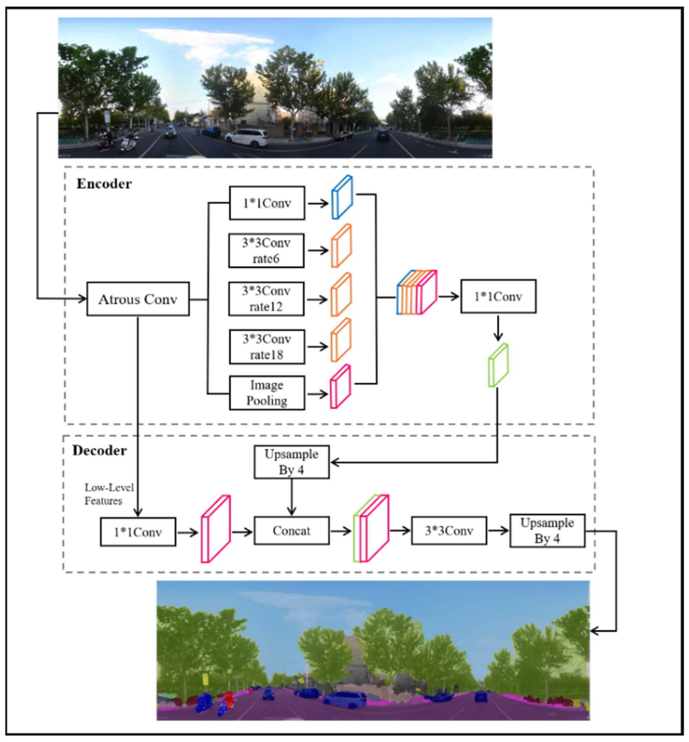
3.1. Semantic Segmentation

Within the domain of computer vision, semantic segmentation is a key goal aimed at classifying each pixel of the image into a predefined semantic category [11]. Distinct from conventional image classification approaches, semantic segmentation needs both identifying visual elements within the imagery and assigning each pixel to its corresponding semantic category, such as buildings, plants, roads, pavements, cars, and pedestrians.

In this study, DeepLabv3+ model [35] is used for semantic segmentation of street view images captured in Shanghai’ main city in order to extract micro-environmental features such as road coverage rate, building coverage rate, green view index, and openness ratio. DeepLabv3+ is a deep learning model based on Convolutional Neural Networks (CNNs), which is one of the best-performing techniques for semantic segmentation [36]. The model improves on its predecessor DeepLabv3 by adopting an Encoder–Decoder structure, which effectively improves the segmentation of image details. The core of DeepLabv3+ is Atrous Convolution and Atrous Spatial Pyramid Pooling (ASPP), which are capable of expanding the sensory field without reducing the image resolution, thus better capturing the features of multi-scale objects in street view images. Atrous convolution can expand the receptive field to capture image features at different scales more comprehensively by introducing a dilation rate in the convolution process, while the ASPP component significantly improves the model’s capability to recognize objects in the scene through multi-scale feature extraction. This approach is especially suitable for identifying objects with significant variations in size in images, such as distant buildings and nearby vegetation. Meanwhile, the decoder part of DeepLabv3+ enhances the resolution and accuracy of semantic segmentation by integrating the feature maps from the encoder with an up-sampling operation, enabling accurate recovery of image edges and details.

The architectural framework of DeepLabv3+ and segmentation effect of the sample data are illustrated in Figure 3. From the sample effect image, we can observe that the model accurately segments various elements, such as sky, buildings, vehicles, roads, and trees. Meanwhile, we extracted the proportions of different elements in images to facilitate further analysis.

3.2. XGBoost

As a Boosting-based model in ensemble learning, XGBoost builds strong learners with improved predictive accuracy by iteratively optimizing multiple weak learners [37]. In each iteration, the model weights the samples according to the residuals of the previous round, giving more focus to samples with higher prediction errors and effectively handling noise and outliers in the data. This weighting mechanism makes XGBoost show strong robustness on complex datasets. Additionally, XGBoost adopts incremental computation and parallel processing techniques to significantly enhance training efficiency. In the paper, we use the XGBoost model to explore the influence of environmental elements on vitality, aiming to identify and quantify the key factors influencing urban vitality. The independent variables of the model consist of 12 built environment factors spanning both micro- and macro-level data, while the dependent variable is urban vitality. By learning the relationships between these independent and dependent variables, the XGBoost model can effectively predict urban vitality in different built environments.

XGBoost can catch complex interactions across features and optimize prediction results by combining multiple decision trees. In each iteration, XGBoost adjusts the model according to the loss function so that each subsequent tree better corrects the errors of the previous round, which is expressed as follows:

$${\widehat{y}}_i^{\left(t\right)}={\displaystyle \sum _{m=1}^t{f}_m}\left(x_i\right)={\widehat{y}}_i^{\left(t-1\right)}+f_t\left(x_i\right)$$

(1)

where m is the mth tree, x_i is the built environment factor of the ith sample, ${\widehat{y}}_i^{\left(t\right)}$ is the predicted value of urban vitality of sample i after t iterations, and f_m(x_i) is the projected result of the mth tree. By continuously iterating and updating the predicted values, the model gradually improves the prediction accuracy of urban vitality.

To prevent overfitting, XGBoost controls the model complexity by bringing in a regularization term. The objective function comprises two distinct components: a loss function l, which examines the deviation between the model’s predicted and real values, and a regularization term Ω(f), which serves as a parameter to constrain model complexity. The objective function L is as follows:

$$L={\displaystyle \sum _{i=1}^{n}l\left(y_i,{\widehat{y}}_i\right)}+{\displaystyle \sum _{m=1}^t\Omega \left(f_m\right)}$$

(2)

$$\Omega \left(f_m\right)=\gamma M+{\displaystyle \frac{1}{2}}\lambda {\displaystyle \sum _{j=1}^M{w}_j^2}$$

(3)

where the true value y_i is the actual vigor of sample i, ${\widehat{y}}_i$ is the vigor predicted by the model, $l\left(y_i,{\widehat{y}}_i\right)$ is the loss function between the predicted and real values describing the difference between them, Ω(f_m) is a regularization term that prevents the model from overfitting, γ is the penalty coefficient used to limit the model’s complexity, M is the number of leaf nodes, λ is the penalty coefficient for the score of leaf nodes used to control the L2 regularization strength of leaf node scores in the model, and w_j is the score of the jth leaf node.

3.3. Shapley Additive Explanations Model

XGBoost is well suited for nonlinear problems as it effectively captures complex nonlinear relationships among features. Nevertheless, the inherent opacity of machine learning models frequently leads to limited explanatory capacity, thereby hindering precise quantification of individual feature contributions to the predictive outcomes. To overcome this methodological constraint, the research implements SHAP framework for model interpretation. SHAP is a game-theoretical-based explanatory framework for interpreting the output of machine learning models [38]. The fundamental principle involves quantifying the contribution of every feature to the predictive results of the model by assigning importance scores to those features. SHAP draws on the notion of Shapley values and aims to fairly distribute benefits of cooperation [39]. Specifically, SHAP synthesizes all potential feature permutations by calculating the marginal contributions of features in different subsets to obtain the global and local importance of each feature. This approach has a solid theoretical foundation and satisfies key properties such as symmetry and consistency, providing a consistent and intuitive explanation for the predictions of complex models [40]. In the computational process, SHAP first generates a background dataset to simulate the real data distribution and then combines it with Monte Carlo methods or other approximation algorithms to improve computational efficiency. This approach is suitable for analyzing the interpretation of tree models, deep learning models, and other nonlinear machine learning models [41]. Recently, SHAP has been widely used in the domains of biomedicine, financial risk assessment, and transportation, providing a powerful tool for studies on model interpretability [42]. In the research, the SHAP model is used to evaluate the influence of environmental features on the prediction outcomes to improve model interpretability and assist in optimizing decision-making. The SHAP value is calculated by the following equation:

$$SHA{P}_{ij}={\displaystyle \sum _{S\subseteq \left\{x_1,x_2\cdots ,x_n\right\}\backslash \left\{x_j\right\}}\frac{\left|S\right|!\left(n-\left|S\right|-1\right)!}{n}}\left(f\left(S\cup \left\{x_j\right\}\right)-f\left(S\right)\right)$$

(4)

where SHAP_ij denotes the SHAP value of the ith sample in feature j, j denotes a built environment indicator, S denotes the feature subset of the model for all possible permutations of built environment indicators other than X_j, and n is the number of built environment indicators.

Additionally, the SHAP summary plot is an important visualization tool, capable of quantifying the average extent to which each feature contributes to the model’s predicted outcomes. Within the swarm visualization plot, individual data points correspond to the specific Shapley value for a single sample, with the vertical axis denoting the features and the horizontal axis representing the amplitude of these values, reflecting the extent to which the feature values influence the model’s predicted outcomes. The color of each point typically represents the actual value taken by the feature. The SHAP summary plot helps identify important features, and features with a broader distribution along the horizontal axis tend to be more influential. It also reveals the direction of influence of feature values and helps to understand their distributions. Overall, the SHAP summary plot provides an effective and intuitive way to comprehensively analyze the association between features and model predictions in machine learning models.

4. Results

4.1. Model Performance

To verify the fitting effect of the XGBoost model constructed in this paper, GBDT and the random forest model are developed as comparison models. During model estimation, the dataset is split into an 80% training set and a 20% test set, where the test set serves to evaluate the generalization ability of models. In the process of applying machine learning algorithms, GridSearchCV combined with cross-validation is used to optimize the hyperparameters and minimize the prediction error. In terms of parameter settings, we set the number of decision trees (100, 200, and 300), the learning rate (0.01, 0.05, and 0.1), the maximum tree depth (3, 4, and 5), the column sampling rate (0.7, 0.8, and 0.9), and the subsampling rate (0.7, 0.8, and 0.9). Ultimately, the most effective parameter configuration for maximizing model efficacy is identified through systematic optimization, with decision trees, learning rate, maximum tree depth, column adoption rate, and subsampling rate set to 100, 0.05, 3, 0.8, and 0.8, respectively. During the optimization process, the maximum depth and learning rate demonstrate substantial influence on the model’s predictive precision. The number of decision trees is implemented to 100 to balance accuracy and efficiency. Additionally, the column sampling rate and subsampling rate are both set to 0.8 for optimal performance. The leaf node splitting threshold is set to 0, indicating that no additional control over node splitting loss is required.

For a thorough assessment of the model’s predictive capabilities, this paper utilizes RMSE, MSE, and R² in the evaluation process. The corresponding outcomes are presented in

Table 2. Model comparison.

Model Name	R2	RMSE	MSE
GBDT	0.315	185.699	34,484.40
Random forest	0.359	179.658	32,276.92
XGBoost	0.432	169.173	28,619.50

. We can find that in the empirical analysis of urban vitality prediction, considerable variations exist in the forecasting effects across different models. The XGBoost model achieves the highest R² of 0.432, representing improvements of 37.14% and 20.33% compared to GBDT and random forest, respectively, indicating that it has the highest goodness-of-fit and superior explanatory ability. The RMSE value of XGBoost is 169.173, which is 8.90% and 5.84% lower compared to GBDT and random forest, respectively, indicating that it has the best stability in prediction results. Since the XGBoost model showed strong performance across all indexes (R², RMSE, and MSE), it was chosen in this study.

4.2. Relative Importance of Built Environment Elements

Figure 4 illustrates the relative importance of various built environment elements in Shanghai’s central area in terms of their impact on vitality. In particular, Figure 4a demonstrates the contributions (measured by SHAP values) and relative importance rankings of the 12 built environment elements. Figure 4b combines the importance of these elements and their impacts on urban vitality. The points in the figure represent the predicted impacts of built environment elements on individual samples, as measured by SHAP values. Sample dots with identical SHAP values are stacked vertically.

As can be seen in Figure 4a, the top six built environment factors in terms of relative importance are the building coverage rate, population density, distance to CBD, the number of metro stations, the openness ratio, and the number of tourist attractions. Among them, the building coverage rate, population density, and distance to CBD have the most significant impact on the model’s prediction of urban vitality. On the other side, the green visibility ratio and the number of bus stops are the least influential elements. In exploring the associations between vitality and built environment variables, the distribution of SHAP values was analyzed. Figure 4b shows the distribution of SHAP values for different variables, revealing the positive and negative feedback effects of each factor on the target variable. The sum of absolute SHAP values decreases gradually from top to bottom. Each color point denotes a separate sample, and the color’s shade reflects the magnitude of feature values for various built environment variables. Taking building coverage rate as an example, locations with a higher building coverage rate in the region show positive SHAP values, indicating that vitality demonstrates elevated levels in regions characterized by greater building density and development intensity. The SHAP values of distance to the CBD are lower than those of the building coverage rate and concentrated on the right side of the x-axis on the graph. This indicates greater urban vitality in areas closer to the CBD. In addition, since the mainstay of urban vitality is people, which are more affected by population density, more densely populated areas also generally show positive SHAP values. The finding aligns with most existing studies [17,43]. Overall, the building coverage rate, population density, the number of metro stations, the number of tourist attractions, road network density, and intersection density have a positive influence on vitality, while distance to CBD and the openness ratio have a negative impact. Other built environment factors show a relatively weak feedback mechanism on urban vitality.

4.3. Nonlinear Association Analysis

Figure 5 uses the SHAP scatterplot to hold a detailed analysis of the association between vitality and environmental elements in which each point represents an observation sample. The right chromaticity bar indicates the magnitude of the SHAP value, and the horizontal coordinates correspond to the eigenvalues of environmental variables. As illustrated in Figure 5a, the SHAP value changes from negative to positive as the building coverage ratio increases. When the building coverage rate exceeds 18%, it has a positive effect on vitality with increasing marginal effects, indicating that a higher building coverage rate contributes to greater economic agglomeration and vitality.

Figure 5b shows that the SHAP value increases gradually as the population density rises, indicating a significant positive correlation between the two. Specifically, when the population density is below 20,000 people/km², the SHAP value is negative, suggesting that a lower population density is not sufficient to support business activities and social interactions. Meanwhile, when it increases from 0 to 26,000 people/km², the urban vitality is significantly improved. However, the improvement becomes relatively weaker when the population density exceeds 26,000 people/km².

Figure 5c demonstrates the correlation between distance to CBD and vitality, which can be divided into two stages according to a threshold value of 1 km. Within 0 to 1 km, the SHAP value improves as the distance increases. However, when the distance exceeds 1 km, a significant negative correlation begins to appear, with the average SHAP value decreasing as distance to the CBD increases. This indicates that, within a certain range, the closer to the CBD, the higher the vitality is. This result aligns with findings from the existing literature [44]. Because the CBD serves as the core business area of the city, it tends to concentrate a large number of commercial, financial, cultural, and other resources, showing a high degree of attraction and radiating influence. Being closer to the CBD makes it easier to access the convenience and opportunities brought by these resources, thus promoting population movement, economic activities and social interactions, and urban vitality enhancement. However, within the range of 0 to 1 km, the SHAP value decreases as the distance to the CBD shortens, which instead negatively effects urban vitality. This might be due to the high volume of traffic and road congestion in the core area of the CBD, which can lower travel efficiency and subsequently impact residents’ quality of life and work productivity, ultimately detracting from the vitality of the city. In addition, housing prices tend to be higher in the CBD area, which leads some residents and businesses to prefer living and operating slightly farther away from the CBD, further inhibiting urban vitality in the core area.

Figure 5d displays the influence of subway stations on vitality, with positive SHAP values when there is a metro station and negative ones when there is no metro station. This suggests that the presence of metro stations can enhance urban vitality because areas with metro stations attract more people and business activities due to the convenience of transport, thus increasing people’s willingness to travel to a certain extent [45], which in turn boosts urban vitality.

The association between the openness ratio and vitality is shown in Figure 5e, which can be approximately divided into two stages according to a threshold value of 0.4. When the openness ratio is less than 0.4, the SHAP value is positive, positively influencing urban vitality. However, when the openness ratio exceeds 0.4, the SHAP value becomes negative, indicating that an excessive openness ratio negatively affects vitality. This might be attributed to insufficient support for commercial activities and social interactions due to inadequate building density and public space.

Figure 5f shows the relationship between the number of tourist attractions and vitality. As the number of tourist attractions increases, the SHAP value increases gradually, and when the number of tourist attractions exceeds 5, the SHAP value increases significantly. However, once it exceeds the threshold value of 10, the SHAP value tends to stabilize, which suggests that the impact of the change in the number of tourist attractions on vitality diminishes after the threshold value is exceeded.

Figure 5g shows the association between road network density and vitality. When it is below 50,000 m/km², the SHAP value is negative, indicating that lower road network density cannot meet the accessibility and connectivity requirements of the city, making it difficult to create spatial vitality. Conversely, when road network density is between 60,000 and 100,000 m/km², the SHAP value significantly increases, indicating that within this range, the increase in road network density can significantly enhance urban vitality.

Figure 5h shows that as the road coverage rate increases, the SHAP value initially increases before decreasing, reaching a maximum when the road coverage rate reaches 12%. When the road coverage rate exceeds the threshold of 14%, the SHAP value becomes negative, suggesting that an excessive road coverage rate can negatively affect urban vitality. This is mainly because excessive road construction potentially damages the urban ecological environment and affects residents’ quality of living, which in turn reduces urban vitality. Another possible reason is that a higher road coverage rate typically implies wider roads in the area, and excessive traffic flow is not friendly to pedestrians, potentially increasing the safety risks for them to a certain extent. When the road coverage rate exceeds 10%, the SHAP value is positive, with sample points concentrated in the 10–14% range, which is a stage that shows a positive impact on vitality and satisfies both traffic accessibility and resident comfort.

Figure 5i illustrates a clear nonlinear association between land-use entropy and vitality, showing a threshold effect. With the increase in land-use entropy, the SHAP value initially increases steadily and then decreases significantly. When entropy falls between 0.6 and 0.87, the SHAP value positively affects vitality, indicating that an increase in entropy value can enhance the diversification of land use. The mixed use of land with different functions, such as the organic combination of commercial, residential, office, and leisure spaces, can satisfy people’s diversified needs within a smaller spatial scope, thus attracting more people and positively contributing to urban vitality. When land-use entropy exceeds the threshold value of 0.87, the SHAP value becomes negative, negatively affecting urban vitality. This indicates that when land-use entropy is too high, excessive diversification and the mixed use of land lead to mutual interference and conflict among different functions, thereby inhibiting urban vitality. For instance, having too many commercial and recreational facilities concentrated in one area can generate noise, traffic congestion, and other issues that negatively impact residents’ quality of life and urban vitality. In addition, excessive mixing also results in disorder and confusion within urban space, reducing the overall image and attractiveness of the city.

Figure 5j shows that as intersection density increases, the SHAP value changes from negative to positive and then turns negative again. When the intersection density exceeds 1200 intersections/km², the SHAP value becomes negative and tends to stabilize. This indicates that when intersection density reaches a certain level, it will have a negative influence on the vitality. This might be because excessive intersection density will lead to serious traffic congestion and environmental issues. In addition, a high intersection density increases the risk of traffic accidents, posing a hazard to the safety and order of the city, which in turn affects its vitality.

The correlation between the green view index and urban vitality is shown in Figure 5k. When the green view index is below 20%, the SHAP value is negative, indicating that insufficient green vegetation leads to poor environmental quality, making it difficult for people to experience pleasure and relaxation, which is detrimental to the enhancement of urban vitality. As the green view index increases, the SHAP value gradually becomes positive. When the green view index exceeds the threshold of 24%, the SHAP value decreases and then tends to stabilize within the positive range, indicating that further increases in the green view index weaken the marginal effect on vitality.

Figure 5l shows a roughly positive association between the number of bus stops and urban vitality, with the SHAP value increasing in stages. When the number reaches 14, the SHAP value rises significantly, indicating that urban vitality notably increases in spaces with an elevated density of bus stops. This is due to the fact that a convenient public transport system attracts more commercial and residential projects, while it also facilitates the movement of people and economic activities, contributing positively to urban vitality.

5. Discussion

In this study, to address the shortcomings of linear models, we break through the traditional linear assumptions and employ the XGBoost model to explore the potential nonlinear relationship between the built environment and urban vitality. Meanwhile, due to the lack of interpretability of machine learning models, we introduce the SHapley Additive exPlanations (SHAP) method to visualize the results and improve the transparency and readability of the model. Unlike previous single-scale research, we use diverse datasets from multiple sources, extracting micro-level data based on semantic segmentation methods and street view images to compare and analyze the distribution of urban vitality in Shanghai’s main urban region at both micro and macro-scales. The results show that there is a nonlinear association and a threshold effect between the built environment and urban vitality. This provides new ideas for subsequent research on the influence mechanism of the built environment on urban vitality, bridges the gaps in the existing literature, and also offers useful guidance for refined urban planning. This helps to make a superior allocation of urban resources and rationally determine the intensity of development and construction, functional layout, and traffic accessibility. At the same time, this can further strengthen the linkages and interactions within the city, facilitating the improvement of urban vitality and sustainable development.

Regarding the planning recommendations, the results of the study can provide a more refined reference basis for built environment planning decisions to enhance urban vitality, especially the range of values of built environment elements that can better guide the optimal allocation of spatial resources (for example, above the highest threshold, the marginal effect of resources decreases; below the lowest threshold, the marginal effect of resources is not triggered). By analyzing the mechanism of the built environment’s influence on urban vitality, we propose the following suggestions.

When the openness ratio is lower than 0.4, it has a positive effect on vitality. Therefore, street design should refer to this threshold to rationally arrange the building heights and layouts, ensuring that public spaces have appropriate sky view and good lighting. At the same time, building density and public spaces should be sufficient to support both commercial activities and social interactions. The contribution to vitality is highest when the green view index is around 0.24, and this threshold should be referred to in planning to achieve a balance between enhancing urban environmental quality and maintaining functionality. The road coverage rate shows a positive impact on vitality in the range of 10 to 14%, which may be a reasonable range to satisfy traffic accessibility and resident comfort and, therefore, should be maintained in planning whenever possible. In addition, it is necessary to rationally plan the type of land use in the region; when the land-use entropy is between 0.6 and 0.87, its positive impact on vitality gradually increases, and the marginal effect is smooth. The planning should consider the use of business type agglomeration to enhance the vitality of the city while avoiding the problems that excessive agglomeration may bring. It should consider the type, scale, and layout of land use to create a vibrant street environment that ensures a good quality of life for residents. At the same time, to meet the accessibility and connectivity of the city, it is possible to increase and optimize road intersections, set appropriate road grades, and increase the density of the pedestrian network, facilitating the movement of vehicles and pedestrians, thus improving urban vitality.

Although this study holds unique value, there are several limitations. Firstly, as the case study focuses on Shanghai’s central urban region, the thresholds and conclusions obtained are broadly applicable to other cities, but their applicability needs further verification since the features and considerations of vitality might vary considerably from one region to another. For more comprehensive investigations and hypothesis verification, subsequent research could extend the geographical coverage by applying the methodology, allowing its validity and universality to be assessed through the use of data from multiple cities or countries. Secondly, the research focuses only on characterizing dynamic population density, which can be further extended by integrating multiple dimensions of vitality, encompassing economic, social, and cultural aspects. Lastly, although we provided an initial explanation of the nonlinear findings using the SHAP model, we have not yet gone further to explore the potential interactions between multiple variables. Consequently, future work should focus on exploring these interactions to gain a more comprehensive understanding of their impact mechanisms.

6. Conclusions

This research uses multi-source data to scientifically construct a systematic refinement of the independent variable indicator system, from both micro and macro-scales, and applies machine learning algorithms combined with SHAP interpretable methods to investigate the nonlinear influence and threshold effects of the built environment on urban vitality in Shanghai’s main urban area. To address the shortcomings of linear models, we break through the traditional linear assumption to tap into potentially complex nonlinear relationships. The visualization of the results improves the transparency and readability of models. The application of multi-scale analysis effectively compensates for the lack of street space details in traditional studies. The analytical outcomes of this study provide valuable insights for optimizing the spatial layout and resource allocation within urban settings, offering references for urban planning and sustainable development initiatives. The following conclusions are drawn:

(1)

There is spatial heterogeneity in the distribution of urban vitality in Shanghai’s main urban area, with the high value of vitality distributed in Huangpu District and the surrounding intersections with various districts to the west, and the vitality exhibits a radial decay pattern emanating from central zones towards peripheral areas.

(2)

Compared to the GBDT and random forest models, the XGBoost model fits better and shows higher performance in simulating and predicting urban vitality.

(3)

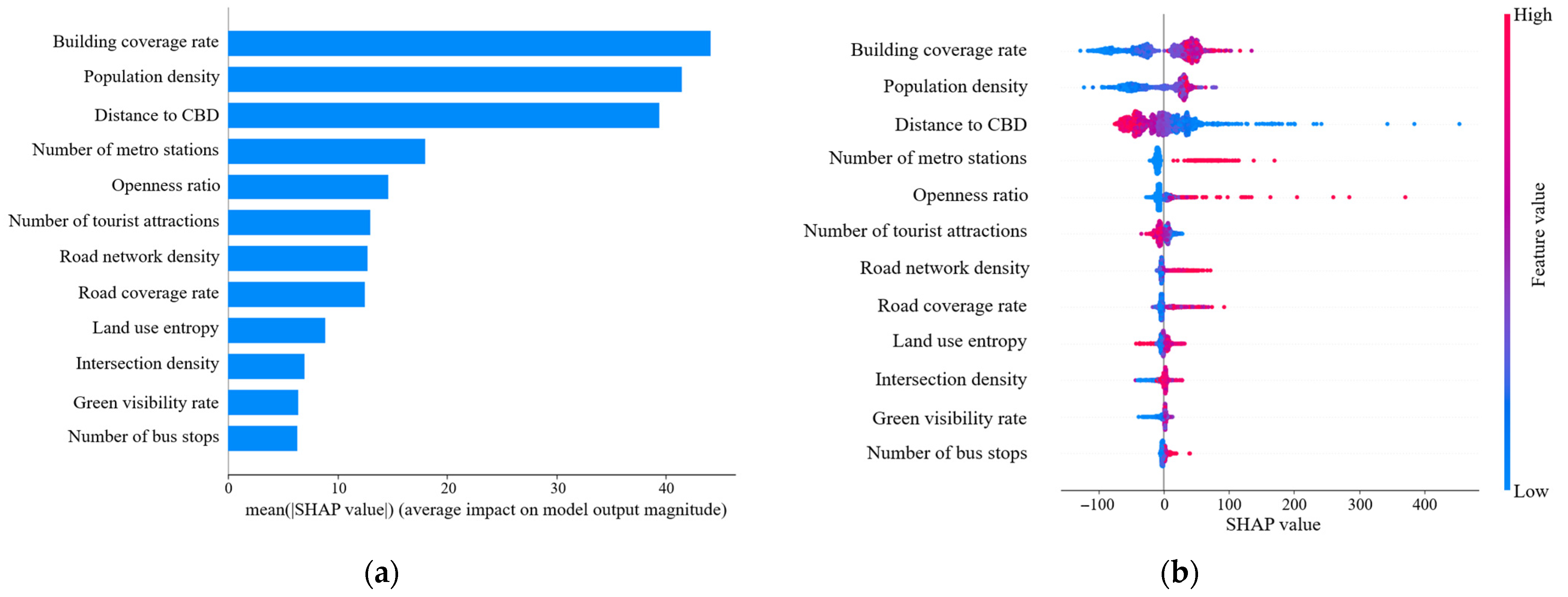
Among all environmental elements affecting urban vitality in Shanghai’s main urban area, the top three in terms of relative importance are building coverage, population density, and distance to the CBD, which exert the most significant effects, while the green view index and the number of bus stops have a relatively low contribution to urban vitality. Building coverage has the largest positive effect on urban vitality, and distance to the CBD exhibits the largest negative correlation with urban vitality.

(4)

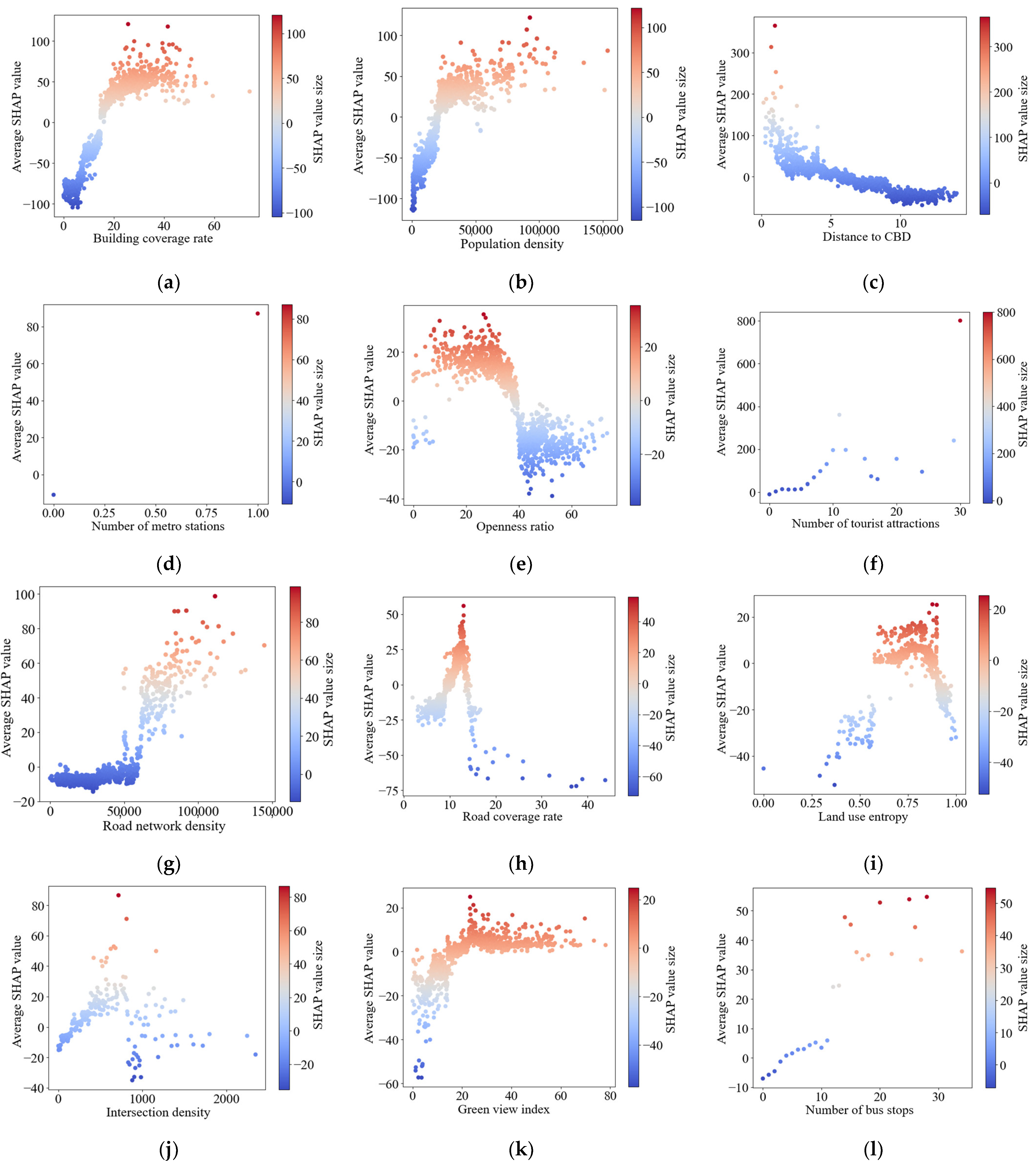
The study based on SHAP value analysis shows that each factor of the built environment has a nonlinear effect on urban vitality and presents a specific threshold value. The nonlinear and threshold effects of urban vitality offer a quantitative analysis tool for urban planning, facilitating one to reasonably allocate resources, especially the range of values of built environment factors that can better guide the optimization of spatial resources.

References

1. Jacobs, J. The Death and Life of Great American Cities; Vintage: New York, NY, USA, 1961. [Google Scholar]
2. Montgomery, J. Making a city: Urbanity, vitality and urban design. J. Urban Des. 1998, 3, 93–116. [Google Scholar] [CrossRef]
3. Still, B.; Simmonds, D. Parking restraint policy and urban vitality. Transp. Rev. 2000, 20, 291–316. [Google Scholar] [CrossRef]
4. Pan, J.; Zhu, X.; Zhang, X. Urban vitality measurement and influence mechanism detection in China. Int. J. Environ. Res. Public Health 2022, 20, 46. [Google Scholar] [CrossRef]
5. Liu, Y.; Liu, X.; Gao, S.; Gong, L.; Kang, C.; Zhi, Y.; Shi, L. Social sensing: A new approach to understanding our socioeconomic environments. Ann. Assoc. Am. Geogr. 2015, 105, 512–530. [Google Scholar] [CrossRef]
6. Talen, E.; Jeong, H. Does the classic American main street still exist? An exploratory look. J. Urban Des. 2019, 24, 78–98. [Google Scholar] [CrossRef]
7. Lee, S.H.; Kang, J.E. Impact of particulate matter and urban spatial characteristics on urban vitality using spatio-temporal big data. Cities 2022, 131, 104030. [Google Scholar] [CrossRef]
8. Cai, J.; Huang, B.; Song, Y. Using multi-source geospatial big data to identify the structure of polycentric cities. Remote Sens. Environ. 2017, 202, 210–221. [Google Scholar] [CrossRef]
9. Wu, C.; Ye, X.; Ren, F.; Du, Q. Check-in behaviour and spatio-temporal vibrancy: An exploratory analysis in Shenzhen, China. Cities 2018, 77, 104–116. [Google Scholar] [CrossRef]
10. Zhang, P.; Zhang, T.; Fukuda, H.; Ma, M. Evidence of multi-source data fusion on the relationship between the specific urban built environment and urban vitality in Shenzhen. Sustainability 2023, 15, 6869. [Google Scholar] [CrossRef]
11. Ma, Z. Deep exploration of street view features for identifying urban vitality: A case study of Qingdao city. Int. J. Appl. Earth Obs. Geoinf. 2023, 123, 103476. [Google Scholar] [CrossRef]
12. Kruse, J.; Kang, Y.; Liu, Y.N.; Zhang, F.; Gao, S. Places for play: Understanding human perception of playability in cities using street view images and deep learning. Comput. Environ. Urban Syst. 2021, 90, 101693. [Google Scholar] [CrossRef]
13. Chen, C.; Wang, J.; Li, D.; Sun, X.; Zhang, J.; Yang, C.; Zhang, B. Unraveling nonlinear effects of environment features on green view index using multiple data sources and explainable machine learning. Sci. Rep. 2024, 14, 30189. [Google Scholar] [CrossRef] [PubMed]
14. Ewing, R.; Cervero, R. Travel and the built environment: A meta-analysis. J. Am. Plan. Assoc. 2010, 76, 265–294. [Google Scholar] [CrossRef]
15. Yang, J.; Cao, J.; Zhou, Y. Elaborating non-linear associations and synergies of subway access and land uses with urban vitality in Shenzhen. Transp. Res. Part A Policy Pract. 2021, 144, 74–88. [Google Scholar] [CrossRef]
16. Yin, C.; Gui, C.; Wen, R.; Shao, C.; Wang, X. Exploring heterogeneous relationships between multiscale built environment and overweight in urbanizing China. Cities 2024, 152, 105156. [Google Scholar] [CrossRef]
17. Lyu, G.; Angkawisittpan, N.; Fu, X.; Sonasang, S. Investigating the relationship between built environment and urban vitality using big data. Sci. Rep. 2025, 15, 579. [Google Scholar] [CrossRef]
18. Yin, C.; Shao, C. Revisiting commuting, built environment and happiness: New evidence on a nonlinear relationship. Transp. Res. Part D Transp. Environ. 2021, 100, 103043. [Google Scholar] [CrossRef]
19. Gao, M.; Fang, C. Deciphering urban cycling: Analyzing the nonlinear impact of street environments on cycling volume using crowdsourced tracker data and machine learning. J. Transp. Geogr. 2025, 124, 104179. [Google Scholar] [CrossRef]
20. Yang, L.; Yang, H.; Yu, B.; Lu, Y.; Cui, J.; Lin, D. Exploring non-linear and synergistic effects of green spaces on active travel using crowdsourced data and interpretable machine learning. Travel Behav. Soc. 2024, 34, 100673. [Google Scholar] [CrossRef]
21. Liu, Y.; Li, Y.; Yang, W.; Hu, J. Exploring nonlinear effects of built environment on jogging behavior using random forest. Appl. Geogr. 2023, 156, 102990. [Google Scholar] [CrossRef]
22. Wang, X.; Yin, C.; Zhang, J.; Shao, C.; Wang, S. Nonlinear effects of residential and workplace built environment on car dependence. J. Transp. Geogr. 2021, 96, 103207. [Google Scholar] [CrossRef]
23. Cervero, R.; Kockelman, K. Travel demand and the 3Ds: Density, diversity, and design. Transp. Res. Part D Transp. Environ. 1997, 2, 199–219. [Google Scholar] [CrossRef]
24. Li, J.; Li, J.; Yuan, Y.; Li, G. Spatiotemporal distribution characteristics and mechanism analysis of urban population density: A case of Xi’an, Shaanxi, China. Cities 2019, 86, 62–70. [Google Scholar] [CrossRef]
25. Tang, L.; Lin, Y.; Li, S.; Li, S.; Li, J.; Ren, F.; Wu, C. Exploring the influence of urban form on urban vibrancy in Shenzhen based on mobile phone data. Sustainability 2018, 10, 4565. [Google Scholar] [CrossRef]
26. Zhang, X.; Sun, Y.; Chan, T.O.; Huang, Y.; Zheng, A.; Liu, Z. Exploring impact of surrounding service facilities on urban vibrancy using Tencent location-aware data: A case of Guangzhou. Sustainability 2021, 13, 444. [Google Scholar] [CrossRef]
27. Li, X.; Li, Y.; Jia, T.; Zhou, L.; Hijazi, I.H. The six dimensions of built environment on urban vitality: Fusion evidence from multi-source data. Cities 2022, 121, 103482. [Google Scholar] [CrossRef]
28. Sung, H.; Lee, S. Residential built environment and walking activity: Empirical evidence of Jane Jacobs’ urban vitality. Transp. Res. Part D Transp. Environ. 2015, 41, 318–329. [Google Scholar] [CrossRef]
29. Ye, Y.; Li, D.; Liu, X. How block density and typology affect urban vitality: An exploratory analysis in Shenzhen, China. Urban Geogr. 2018, 39, 631–652. [Google Scholar] [CrossRef]
30. Zhang, A.; Xia, C.; Chu, J.; Lin, J.; Li, W.; Wu, J. Portraying urban landscape: A quantitative analysis system applied in fifteen metropolises in China. Sustain. Cities Soc. 2019, 46, 101396. [Google Scholar] [CrossRef]
31. Yang, Z.; Zhang, C.; Li, G.; Xu, H. Analysis of the impact of different road conditions on accident severity at highway-rail grade crossings based on explainable machine learning. Symmetry 2025, 17, 147. [Google Scholar] [CrossRef]
32. Delclòs-Alió, X.; Gutiérrez, A.; Miralles-Guasch, C. The urban vitality conditions of Jane Jacobs in Barcelona: Residential and smartphone-based tracking measurements of the built environment in a Mediterranean metropolis. Cities 2019, 86, 220–228. [Google Scholar] [CrossRef]
33. Ling, Z.; Zheng, X.; Chen, Y.; Qian, Q.; Zheng, Z.; Meng, X.; Shi, X. The nonlinear relationship and synergistic effects between built environment and urban vitality at the neighborhood scale: A case study of Guangzhou’s central urban area. Remote Sens. 2024, 16, 2826. [Google Scholar] [CrossRef]
34. Yang, C.; Xu, F.; Jiang, L.; Wang, R.; Yin, L.; Zhao, M.; Zhang, X. Approach to quantify spatial comfort of urban roads based on street view images. J. Geo-Inf. Sci. 2021, 23, 785–801. [Google Scholar]
35. Chen, L.C.; Zhu, Y.; Papandreou, G.; Schroff, F.; Adam, H. Encoder-decoder with atrous separable convolution for semantic image segmentation. In Proceedings of the European Conference on Computer Vision (ECCV), Munich, Germany, 8–14 September 2018; pp. 801–818. [Google Scholar]
36. Zhang, L.; Wang, L.; Wu, J.; Li, P.; Dong, J.; Wang, T. Decoding urban green spaces: Deep learning and Google Street View measure greening structures. Urban For. Urban Green. 2023, 87, 128028. [Google Scholar] [CrossRef]
37. Chen, T.; Guestrin, C. XGBoost: A scalable tree boosting system. In Proceedings of the 22nd ACM SIGKDD International Conference on Knowledge Discovery and Data Mining, San Francisco, CA, USA, 13–17 August 2016; pp. 785–794. [Google Scholar]
38. Kuhn, H.W.; Tucker, A.W. (Eds.) Contributions to the Theory of Games; Princeton University Press: Princeton, NJ, USA, 1953; No. 28. [Google Scholar]
39. Lundberg, S.M.; Lee, S.I. A unified approach to interpreting model predictions. Adv. Neural Inf. Process. Syst. 2017, 30, 4765–4774. [Google Scholar]
40. Štrumbelj, E.; Kononenko, I. Explaining prediction models and individual predictions with feature contributions. Knowl. Inf. Syst. 2014, 41, 647–665. [Google Scholar] [CrossRef]
41. Lundberg, S.M.; Erion, G.; Chen, H.; DeGrave, A.; Prutkin, J.M.; Nair, B.; Lee, S.I. From local explanations to global understanding with explainable AI for trees. Nat. Mach. Intell. 2020, 2, 56–67. [Google Scholar] [CrossRef]
42. Molnar, C. Interpretable Machine Learning: A Guide for Making Black Box Models Explainable; Lulu.com: Raleigh, NC, USA, 2022. [Google Scholar]
43. Jin, X.; Long, Y.; Sun, W.; Lu, Y.; Yang, X.; Tang, J. Evaluating cities’ vitality and identifying ghost cities in China with emerging geographical data. Cities 2017, 63, 98–109. [Google Scholar] [CrossRef]
44. Tu, W.; Zhu, T.; Xia, J.; Zhou, Y.; Lai, Y.; Jiang, J.; Li, Q. Portraying the spatial dynamics of urban vibrancy using multisource urban big data. Comput. Environ. Urban Syst. 2020, 80, 101428. [Google Scholar] [CrossRef]
45. Sun, B.; Ermagun, A.; Dan, B. Built environmental impacts on commuting mode choice and distance: Evidence from Shanghai. Transp. Res. Part D Transp. Environ. 2017, 52, 441–453. [Google Scholar] [CrossRef]
Figure 1. Study area.
Buildings 15 01414 g001
Figure 2. Spatial pattern of urban vitality in the main urban area of Shanghai.
Buildings 15 01414 g002
Figure 3. Model structure and sample effects.
Buildings 15 01414 g003
Figure 4. Relative importance of environmental elements on vitality. (a) Variable contribution and ranking of relative importance; (b) distribution of SHAP values for variables.
Buildings 15 01414 g004
Figure 5. SHAP scatterplot of variables. (a) The SHAP scatter plot of the building coverage rate; (b) The SHAP scatter plot of the population density; (c) The SHAP scatter plot of the distance to CBD; (d) The SHAP scatter plot of the number of metro stations; (e) The SHAP scatter plot of the openness ratio; (f) The SHAP scatter plot of the number of tourist attractions; (g) The SHAP scatter plot of road network density; (h) The SHAP scatter plot of the road coverage rate; (i) The SHAP scatter plot of land-use entropy; (j) The SHAP scatter plot of intersection density; (k) The SHAP scatter plot of the green view index; (l) The SHAP scatter plot of the number of bus stops.
Buildings 15 01414 g005