Abstract
Machine learning methods are widely used to predict the bearing capacity of concrete-filled steel tubular (CFST) columns. However, in addition to this task, the engineer often faces the inverse problem: to determine what cross-section dimensions of the CFST column are required for given loads. This paper is devoted to the development of machine learning models for predicting the geometric parameters of a circular cross-section for concrete-filled steel tubular (CFST) columns under the combined action of bending moments and compressive axial forces. This problem has not been solved by machine learning methods before. The main focus is on automating the design process of CFST columns using the CatBoost algorithm and artificial neural networks. Three machine learning models were developed to solve the problem. The first and second models are based on the CatBoost algorithm. They predict the column diameter at minimum and maximum wall thicknesses, respectively. The third model is an artificial neural network, which is designed to determine the wall thickness of a CFST column. The models were trained on synthetic data generated in accordance with Russian design codes. The first and second models demonstrated high accuracy in predicting the column diameter (RMSE = 3.86 mm and 4.12 mm, respectively). The third model showed high efficiency over the entire range of wall thicknesses (correlation coefficient R = 0.99974). Feature importance analysis using SHAP values confirmed the key role of bending moment and axial force in predicting geometric parameters.
1. Introduction
Concrete-filled steel tubular (CFST) columns with a circular cross-section, which are the object of this study, are composite structures consisting of an internal concrete core and an external steel shell. In recent decades, these structures have attracted considerable attention, combining the advantages of concrete and steel, providing increased load-bearing capacity [1]. Due to their high mechanical performance, CFST columns are used in super high-rise buildings [2,3,4], bridge structures [5,6], overpasses [7], etc.
The results of CFST column laboratory experimental studies are the most reliable and valid, but they remain limited due to high labor intensity, significant time costs, and the need for complex laboratory equipment [8]. In this regard, a large number of researchers have focused on the construction of numerical models for predicting the bearing capacity of CFST columns [9,10]. It should be noted that the national building codes of many countries are limited by the range of materials used, which reduces their versatility in the design of modern high-strength structures. At the same time, national codes differ significantly in the permissible characteristics of materials. In particular, the Russian (SP 266.1325800.2016) and American (AISC 360) standards allow for the use of stronger steels and concrete, while the European (Eurocode 4) standard introduces more stringent restrictions, which narrows the scope of its application. This difference in the approaches emphasizes the need to develop models that take into account a wide range of possible material characteristics and provide accurate bearing capacity prediction of the columns [11,12].
Predicting the bearing capacity of CFST columns is a complex task that requires many factors to be taken into account, such as the nonlinear behavior of materials, interaction of steel and concrete, and the influence of geometric parameters of the structure. In this regard, numerous studies pay special attention to the development and use of methods based on modern numerical approaches of structural mechanics and theories of deformable solids. Since it is difficult to develop your own FEA system, many authors use existing ones. Among the most popular and proven systems, ABAQUS and ANSYS can be highlighted, which offer a wide range of tools for analyzing the stress–strain state of CFST columns [13,14,15].
The rapid development of artificial intelligence algorithms has influenced the methods of CFST columns’ calculation and design, expanding the possibilities of analyzing deformation processes, assessing strength characteristics, and predicting operational indicators, which is the basis for creating reliable engineering solutions. Various methods and algorithms of artificial intelligence in these studies are used to predict the bearing capacity of CFST columns.
One of the first to use artificial intelligence methods to solve the problem of determining the bearing capacity of CFST columns under axial compression was H. Gao in 2011 [16]. This study proposed a neural network model with back propagation, successfully trained on experimental data for a square cross-section.
However, in the following years, interest in the application of artificial intelligence tools in this area remained limited, and only a few studies confirmed the effectiveness of neural networks for assessing the strength of CFST columns [17,18].
One of the next steps in this direction was the study by M. Ahmadi [19] presented in 2014, in which a new approach was formulated to predict the CFST column axial capacity using an artificial neural network (ANN) model trained using the Levenberg–Marquardt algorithm. A large array of experimental data were analyzed, including parameters such as the yield strength and wall thickness of the steel pipe, concrete strength, and column geometry.
Rectangular CFST columns were investigated by Du Y. [20] with the use of artificial neural networks to predict their axial load-bearing capacity based on 305 experiments, comparing the results with the national standards of different countries. Later, a new approach was proposed by Le T. et al. [21] to predict the ultimate axial load of rectangular columns, also using artificial neural networks, based on data from 880 experiments.
More recent and modern studies demonstrate that the use of ANN remains in demand, continues to improve in terms of the problems of predicting the strength of CFST columns, and demonstrates higher accuracy in predicting the bearing capacity of columns compared to traditional theoretical approaches [22,23,24,25,26]. In particular, in the work in ref. [27], an optimized ANN model for predicting the ultimate axial capacity of CFRP-reinforced CFST columns using both experimental and numerical data is presented. Based on this study [28], it can be concluded that the proposed ANN model for predicting the axial capacity of high-strength concrete circular CFST columns shows superior results compared with the existing national codes (AS/NZS 5100.6, Eurocode 4, AISC, and GB 50936).
Faridmehr I. et al. [29] compared the AISC 360-16 and Eurocode 4 building codes for the calculation of the CFST columns load-bearing capacity, showing the greater accuracy of the European standard and confirming the effectiveness of ANN-based models for high-strength concrete.
In addition to neural networks, a number of studies use classical machine learning (ML) methods, which improves the accuracy and adaptability of models for calculating the strength of CFST. The paper in ref. [30] proposes a model based on Natural Inspired Machine Learning (NIML), which identifies relationships between geometric and physical–mechanical parameters, trained on 3103 trials.
Nguyen T. T. et al. [31] have refined the American standard (ACI 318-08) strength condition based on the analysis of 663 experimental specimens using machine learning, which allows for a more accurate prediction of the compressive strength of CFST columns. Nguyen T.-A. et al. [32,33] developed a universal machine learning model to analyze the influence of geometric and physical–mechanical parameters on the axial bearing capacity of CFST columns. This study was based on a large dataset (3094 observations) and careful model optimization (CatBoost, LightGBM, XGBoost) using grid search and cross-validation.
A comparative analysis of different ML methods for predicting the axial bearing capacity of CFST columns by Lai D et al. [34] revealed the advantages of the Natural Gradient Boosting (NGBoost) algorithm with a lognormal distribution. The proposed approach provided more accurate predictions with minimum overfitting and high stability in comparison with XGBoost, ANN, and XGBD.
Li J. et al. [35] studied the residual bearing capacity (RALBC) of CFST columns after blasting. The analysis of 1599 columns was carried out using the finite element method. XGBoost, ANN, and SVR were used to predict the RALBC. The impact of blast loading is also discussed in the article in ref. [36], which predicts the peak response of CFST columns using machine learning methods. Twelve regression metrics were compared, the Monte Carlo method was applied, and the key factors influencing the response were identified. A similar problem was considered in the work in ref. [37] for H-section steel columns under impulsive blast loads via gene expression programming.
In the paper in ref. [38] by M. Zarringol et al., the prediction of ultimate axial load for rectangular CFRP-reinforced concrete columns is considered using ANN and XGBoost trained on datasets consisting of 64 experimental test results and 296 finite element analysis (FEM) results. XGBoost performed better, providing more accurate and interpretable predictions, while ANN was used to derive an empirical equation that passed the reliability analysis according to the American Standard for Design of Steel Structures (AISC 360-16).
Nishant Arora H. et al., using analytical models and machine learning (ML) algorithms, carried out the evaluation of the axial load-bearing capacity (ALCC) for reinforced concrete (RC) columns strengthened with ferrocement in the work in ref. [39]. A database of 151 samples was used for the analysis. Four machine learning models were developed: ANN, decision tree (DT), linear regression (LR), and support vector machine (SVM), of which the ANN model showed the best results. However, it should be noted that the limited amount of data used to train the models in the works in refs. [38,39] may affect the degree of confidence in the reliability of the results obtained.
In the research in refs. [40,41] by M. Gupta et al. and N. Ngo et al., the artificial neural network with particle swarm optimization (PSO) and with gray wolf optimization (GWO) was used to predict the ultimate axial load of square CFST columns, and the superiority of the combination of artificial neural network and particle swarm optimization was confirmed.
Javed M. et al. presented in paper [42] a new method for calculating the ultimate axial bearing capacity of long circular CFST columns using gene expression programming (GEP). The resulting equation, based on experimental data, allows for the bearing capacity to be calculated manually.
Sarir P. et al. [43] have noted that for predicting the bearing capacity of CFST columns, the XG-Boost method showed the best results compared to ANN and RF (random forest), and such an input parameter as the column diameter has the greatest influence on its bearing capacity.
Narang A. et al. [44,45] made a systematic review and study of four methods for predicting the residual CFST columns’ strength: Gaussian regression (GPR), ensemble methods, support vector machine, and artificial neural networks. The best results were demonstrated by SVM and ANN with coefficients of determination (R2) of 0.93 and 0.98, respectively.
In a study conducted by Y. Lusong et al. [46], it was found that artificial neural network models optimized using the whale optimization algorithm (WOA) showed higher accuracy in predicting axial load for short CFST columns than existing formulas in building codes.
Based on the results of the study in ref. [47] on the assessment of the bearing capacity of CFST with round and square sections, it can also be concluded that the use of genetic programming and artificial neural networks shows high accuracy of model predictions, confirming their consistency with experimental data. At the same time, the authors used a database of 993 samples to develop the models, taking into account the physical, mechanical, and geometric characteristics of the columns.
In the study in ref. [48], two machine learning models, Gaussian process (GPR) and XGBoost, were proposed to solve the problems of rectangular column strength analysis. The models are trained and evaluated on two datasets, including 958 axially loaded columns and 405 eccentrically loaded columns.
K. Megahed et al. [49,50] have proposed various machine learning models for predicting CFST columns’ strength. GPR, XGBoost, symbolic regression (SR), and CatBoost were examined. The GPR and CatBoost models demonstrated the highest accuracy and reliability.
In the paper in ref. [51] by Shen F. et al., the authors point out that predicting the bearing capacity of CFST compressed columns is a complex task due to nonlinear interactions between design parameters. To address this issue, the authors explore the capabilities of machine learning (LightGBM, XGBoost, CatBoost) and deep learning (DNN, CNN, LSTM) methods in comparison with traditional analytical models.
The provided analysis of the conducted studies is summarized in Table 1. It shows that most of the papers are devoted to the assessment of the CFST columns’ bearing capacity using machine learning methods. Machine learning methods can also be used in the optimal design of building structures [52,53,54], but issues related to determining the optimal dimensions of CFST columns’ cross-section remain. The main emphasis in most works is on the assessment of strength characteristics. For a civil engineer, the key task in the design of structures with CFST elements is to determine the required cross-sectional dimensions, in particular the diameter and wall thickness of the steel pipe.

Table 1.
Summary of the literature review.
The calculation methods contained in the current design codes do not provide a direct way to solve the problem of selecting the required diameter and wall thickness of a CFST column. To effectively solve this problem, machine learning (ML) models can be applied. As the review showed, boosting models and artificial neural networks, due to their high accuracy and ability to take into account complex nonlinear data dependencies, are an effective tool for designing CFST columns, providing reliable and interpretable results. This study has as its main objective to fill the research gap, which consists of the absence of algorithms for determining the required cross-sectional dimensions of CFST columns. The aim of this study is to develop ML models for predicting the cross-sectional dimensions of circular CFST columns under the combined action of bending moments and compressive axial forces, taking into account the limitations imposed by Russian design codes.
Under the same loading conditions, there can be multiple design solutions for a single CFST cross-section. In this study, three machine learning models were developed for forecasting. The first model was for the prediction of the column diameter Dp1 at the minimum possible wall thickness of the steel pipe according to the assortment. This option provides the lowest cost due to the minimum consumption of steel, but the cross-sectional diameter is the largest. The second model was for the prediction of the column diameter Dp2 at the maximum possible wall thickness of the pipe. This option corresponds to the minimum possible column diameter. The third model was for the prediction of the wall thickness of the steel pipe with an arbitrary diameter between Dp2 and Dp1. The CatBoost algorithm and the Levenberg–Marquardt optimization algorithm were used to train the models, which improved the forecasting accuracy and automated the design of CFST columns.
2. Materials and Methods
2.1. Machine Learning Models for Predicting Required Cross-Section Diameter
Two machine learning models were developed to predict the required cross-sectional diameter. The first model predicts the required column cross-section diameter when the wall thickness reaches its minimum value according to the assortment of round electric-welded straight-seam pipes GOST 10704-91. The second model predicts the minimum possible column cross-section diameter when the wall thickness reaches its maximum value. The input parameters of the first two models are the values specified in Table 2.
Table 2.
Input parameters of models 1 and 2.
The coefficient , which acts as the sixth input parameter, was determined in accordance with Russian design codes for steel-reinforced concrete structures SR266.1325800.2016 using the following formula:
and here are, respectively, the bending moments from the action of the full load and from the action of constant and long-term loads.
The models were trained using synthetic data. The provisions of SR266.1325800.2016 were used to form the training dataset. According to this regulatory document, the strength condition of CFST elements experiencing the combined action of compressive axial forces and bending moments, in the absence of bar reinforcement, is as follows:
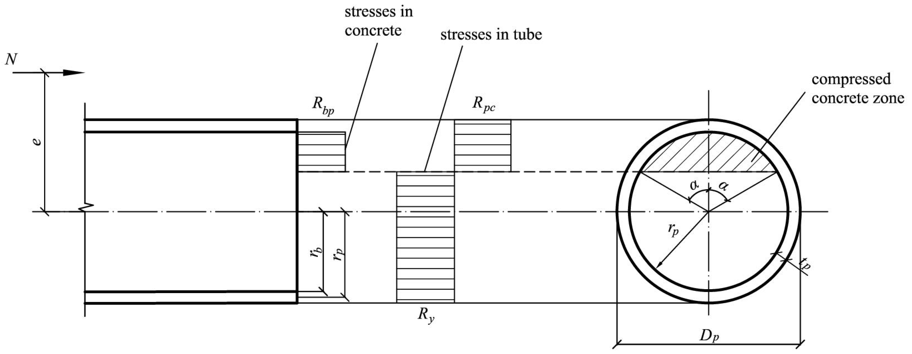
where is the eccentricity of the axial force, is the internal radius of the steel pipe, is the cross-sectional area of the steel shell, is the radius of the steel shell middle surface, and are the calculated strength of concrete and steel under compression as part of a CFST element, and is the angle determining the position of the concrete compressed zone in the ultimate state (Figure 1).
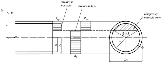
Figure 1.
Limit equilibrium of an eccentrically compressed CFST element.
The quantities and are determined by the following formulas:
where .
The angle in Formula (2) is determined from the condition that the sum of the projections of internal and external forces on the longitudinal axis of the column is equal to zero, which leads to a nonlinear equation:
When determining the eccentricity in Formula (2), in addition to the calculated eccentricity , it is necessary to take into account the random eccentricity , as well as the increase in eccentricity in a slender column due to the deflection of the element. The additional eccentricity caused by the deflection of the element is taken into account using the coefficient :
where is the Euler critical force, and B is the reduced bending stiffness of the cross-section taking into account the development of plastic deformations and creep.
Random eccentricity is defined as the largest of three values: cm; ; .
The value is defined as the minimum of two values:
where , is the moment of inertia for the concrete part of the composite section, is the moment of inertia for the steel shell, MPa is the modulus of the elasticity of steel, and is the long-term concrete modulus of deformation taking into account creep effects.
The value is calculated using the following formula:
where and are, respectively, the initial modulus of elasticity and the creep coefficient of concrete.
There is a correlation between the initial modulus of the elasticity of concrete and its compressive strength. The following formula given in ref. [55] to determine was used:
The creep coefficient of concrete was determined based on the data [56]:
The coefficient that reduces the stiffness of the section due to the plastic work of concrete is determined by the following formula:
where is the relative value of the axial force eccentricity, taken to be no less than 0.15 and no more than 1.5.
The formation of the training dataset for models 1 and 2 was performed according to the following algorithm:
- According to GOST 10704-91 assortment, the range from 102 to 1420 mm was selected for . All intermediate values were used when training the models.
- The ranges for input parameters , , , and were selected, as well as the step with which these input parameters changed (Table 3).
Table 3. Ranges and step of change for input parameters in training datasets for models 1 and 2.
For and , the choice of the specified ranges was determined by the grades of the most common properties, steel and concrete, used in CFST columns. As for the calculated length parameter, columns with a length of less than 10 diameters can be considered short, and for them the deflection does not lead to a noticeable increase in the eccentricity of the axial force. The result of the cross-section dimensions’ prediction for them will be the same as for columns with a length of 10⋅Dp. Columns with a length of more than 30 diameters are very slender structures for which ensuring overall stability is a serious problem. The coefficient based on Formula (1) can vary from 1 to 2.
- 3.
- For each set of values , , , , and at the minimum (for model 1) and maximum (for model 2) wall thickness according to the GOST 10704-91 assortment, the following sequence of actions was performed:
- 3.1.
- The ultimate axial force under central compression was determined without taking into account the slenderness of the element using the following formula:where is the cross-sectional area of the concrete core.The values of and under central compression were determined by the following formula:
- 3.2.
- The ultimate bending moment for pure bending was determined using the following formula:The angle in Formula (13) was calculated from the solution of the following nonlinear equation:The training dataset was written with a row , where the first 6 elements are the input parameters of the model and is the output parameter.
- 3.3.
- A stepwise increase in the axial force N was performed from 0 to with a step . The number of steps by load was taken as equal to 100. The eccentricity of the axial force was initially taken as equal to zero ().
At each step in N, the angle was determined from the solution of Equation (4). Then, the ultimate bending moment was calculated using the second formula in (2). Then, the corrected eccentricity was calculated according to the following formula:
If the difference between and exceeded 1%, then the corrected value of eccentricity was calculated. Taking into account the corrected value , the strength of concrete and steel was corrected according to Formula (3), as well as the angle and value. The iteration process was completed when the difference between and became less than 1%, or the number of iterations exceeded the specified one.
Once the iteration process described above was completed, the next iteration process began. The relative eccentricity was calculated. Then, the coefficient was determined using Formula (10) and the bending stiffness of the cross-section was calculated using Formula (6). Then, the Euler force and coefficient were calculated using the second formula in (5). If the coefficient was negative, it was replaced by a very large positive number (1010). Then, the initial eccentricity was calculated using the following formula:
Next, the corrected value of the relative eccentricity was determined using the following formula:
If the difference between and exceeded 1%, then the corrected value was calculated and the values were recalculated until the required accuracy was achieved.
A row was written regarding the training dataset for each value , provided that was non-negative.
If the value turned out to be negative, then the increase in load was stopped and a transition to the next set of values , , , , and was performed.
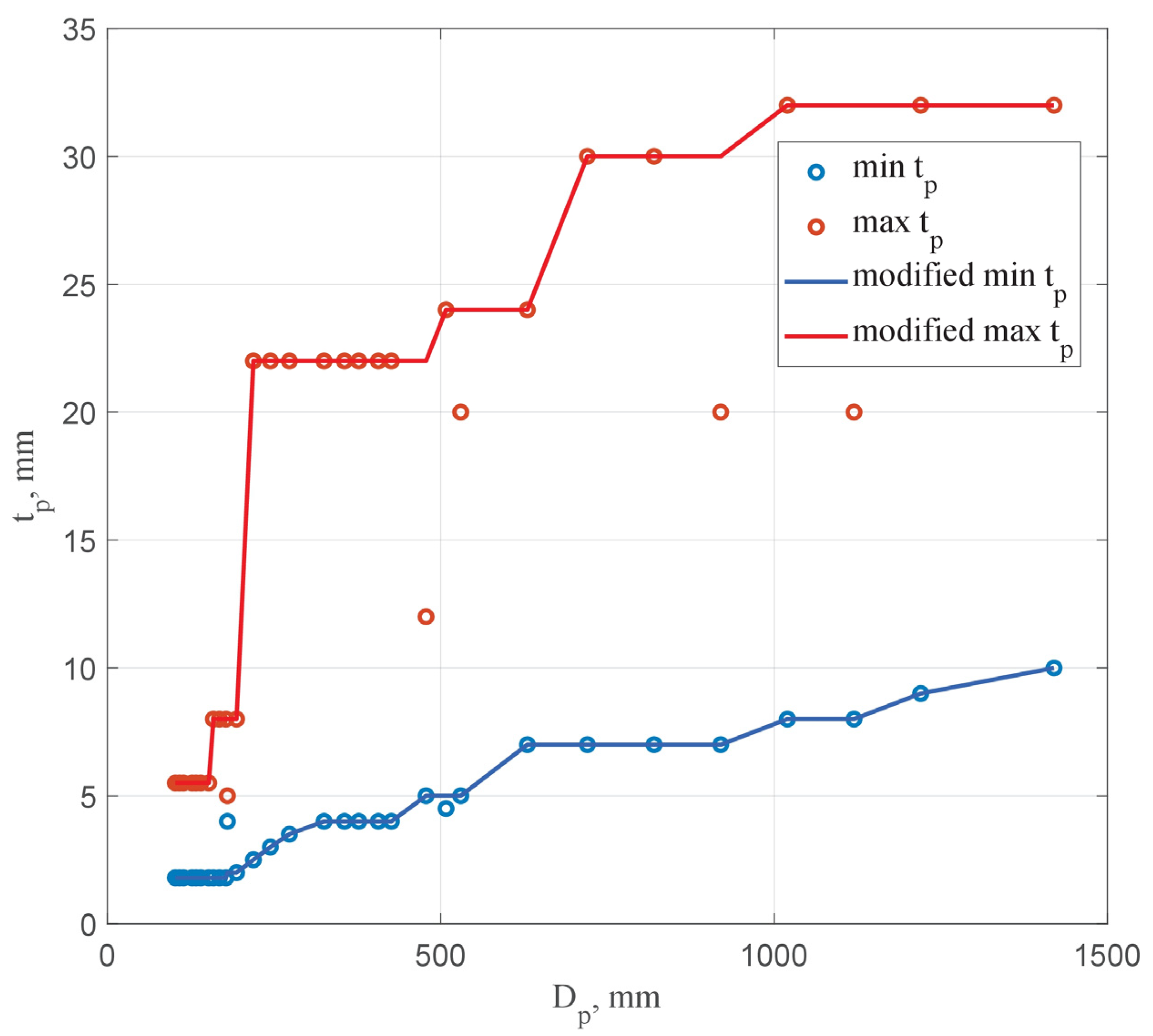
Figure 2 shows graphs of changes in the minimum and maximum wall thickness of a pipe depending on the outside diameter according to the GOST 10704-91 assortment. To ensure the smoothness of the generated data, the dependencies were transformed into non-decreasing functions. The modified graphs are also shown in Figure 2.
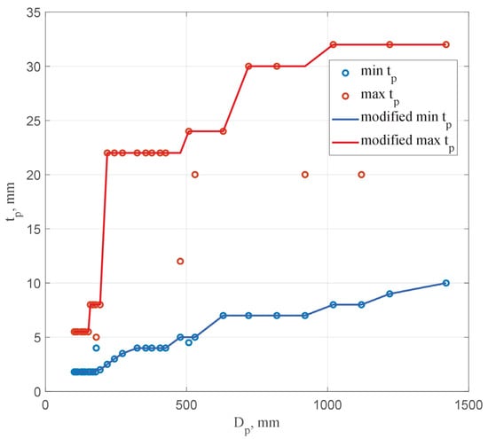
Figure 2.
Change in minimum and maximum pipe wall thickness depending on diameter.
Table 4 and Table 5 show fragments of training datasets for models 1 and 2. The volumes of the first and second datasets were 1,445,552 and 2,055,625 rows, respectively. The statistical characteristics of the generated datasets for models 1 and 2 are given in Table 6 and Table 7. The constraints on the models’ input and output parameters are determined by the minimum and maximum values of the variables in the training datasets specified in these tables.
Table 4.
Fragment of the training dataset for model 1.
Table 5.
Fragment of the training dataset for model 2.
Table 6.
Statistical characteristics of the generated dataset for model 1.
Table 7.
Statistical characteristics of the generated dataset for model 2.
2.2. Machine Learning Model for Determining Required Pipe Wall Thickness
The third model was designed to predict the required pipe wall thickness when a pipe diameter takes an intermediate value between Dp2 and Dp1. The input parameters of model 3 were the values specified in Table 2, as well as the outer diameter of the column . When forming the training dataset for model 3, the pipe wall thickness for each diameter value from the assortment varied from to with a step of . The number of steps by variables was also taken to be 5, and by variable it was 4. The number of steps by axial force was taken to be 20. The algorithm for forming the training dataset for model 3 was similar to the algorithm for models 1 and 2. The only difference was that the values were recorded as input parameters, and the output parameter was the value. A fragment of the training dataset for model 3 is given in Table 8. The total volume of the training dataset for model 3 was 1,037,319 lines. The statistical characteristics of the generated dataset for model 3 are given in Table 9.
Table 8.
Fragment of the training dataset for model 3.
Table 9.
Statistical characteristics of the generated dataset for model 3.
2.3. Machine Learning Algorithms Used to Build Models
Machine learning is the process of establishing patterns between input and output variables based on a training sample [57]. This formulation is a generalization of classical function approximation problems. In our study, the CatBoost (Categorical Boosting) algorithm [58] was used to predict the diameter of CFST columns based on six initial characteristics, and a feedforward artificial neural network model was built to predict the wall thickness of a pipe based on the same six characteristics and diameter, which was trained using the Levenberg–Marquardt algorithm [59,60]. The choice of CatBoost and ANN as machine learning methods was due to their successful application in direct problems of predicting the bearing capacity of CFST columns in the works [16,17,19,20,21,22,23,24,25,27,28,29,31,32,33,40,46,49,50,51].
The CatBoost models were implemented in the Kaggle platform [61] using the Python programming language (version 3.11). The ANN model was implemented in MATLAB R2020b (Deep Learning Toolbox) [62].
The basic concept of gradient boosting is to sequentially build an ensemble of models, each of which learns from the mistakes of the previous ones, which leads to a gradual decrease in the loss function and an increase in the accuracy of predictions.
The application of this method in engineering design problems, in particular for predicting the diameter and wall thickness of CFST columns, shows high efficiency due to the ability to capture complex nonlinear relationships between input and output parameters.
In the context of the task, the CatBoost model is trained on a sample formed on the basis of synthetic data, including many parameters that determine the design and physical–mechanical characteristics of CFST columns. Among such parameters, one can single out loads of various nature, the properties of the materials used, as well as geometric features of the structural elements. Additionally, factors affecting the strength and stability of columns under operational loads are taken into account.
The use of a wide range of input features provided the model with the ability to take into account the complex influence of various factors on target indicators, which are the cross-section diameter or column thickness.
It should be emphasized that an important advantage of the CatBoost algorithm is its resistance to overfitting, achieved through the use of the Ordered Boosting method. Using this approach helps reduce model bias and increase the reliability of predictions, which is of fundamental importance in conditions of limited training data and their high noise level. Given the specifics of predicting the diameter or wall thickness of the CFST columns task, the ability to maintain high accuracy when working with incomplete or limited samples is a significant advantage.
In the context of the previously discussed features of the CatBoost application for predicting the design parameters of CFST columns’ cross-sections, it is necessary to describe in more detail the gradient boosting method used in this study. Let us denote the training sample as follows:
where
- is a vector of features describing the structural and load characteristics of the column (compressive axial force , calculated bending moment , yield strength of steel , design strength of concrete , calculated column length , long-term load factor , and, if necessary, the outer diameter of the column );
- is the target variable corresponding to the predicted parameter (cross-section diameter or pipe wall thickness);
- is the number of observations in the sample;
- is the number of features.
The goal is to find an approximating function that minimizes the loss function :
The boosting method forms an ensemble of weak models (e.g., decision trees) combined as follows:
where
- is the initial prediction, defined as follows:which in the case of regression often corresponds to the mean value of the target variable.
- is a weak model at the m-th step, trained on the mistakes of previous models;
- is the learning coefficient, defined as follows:
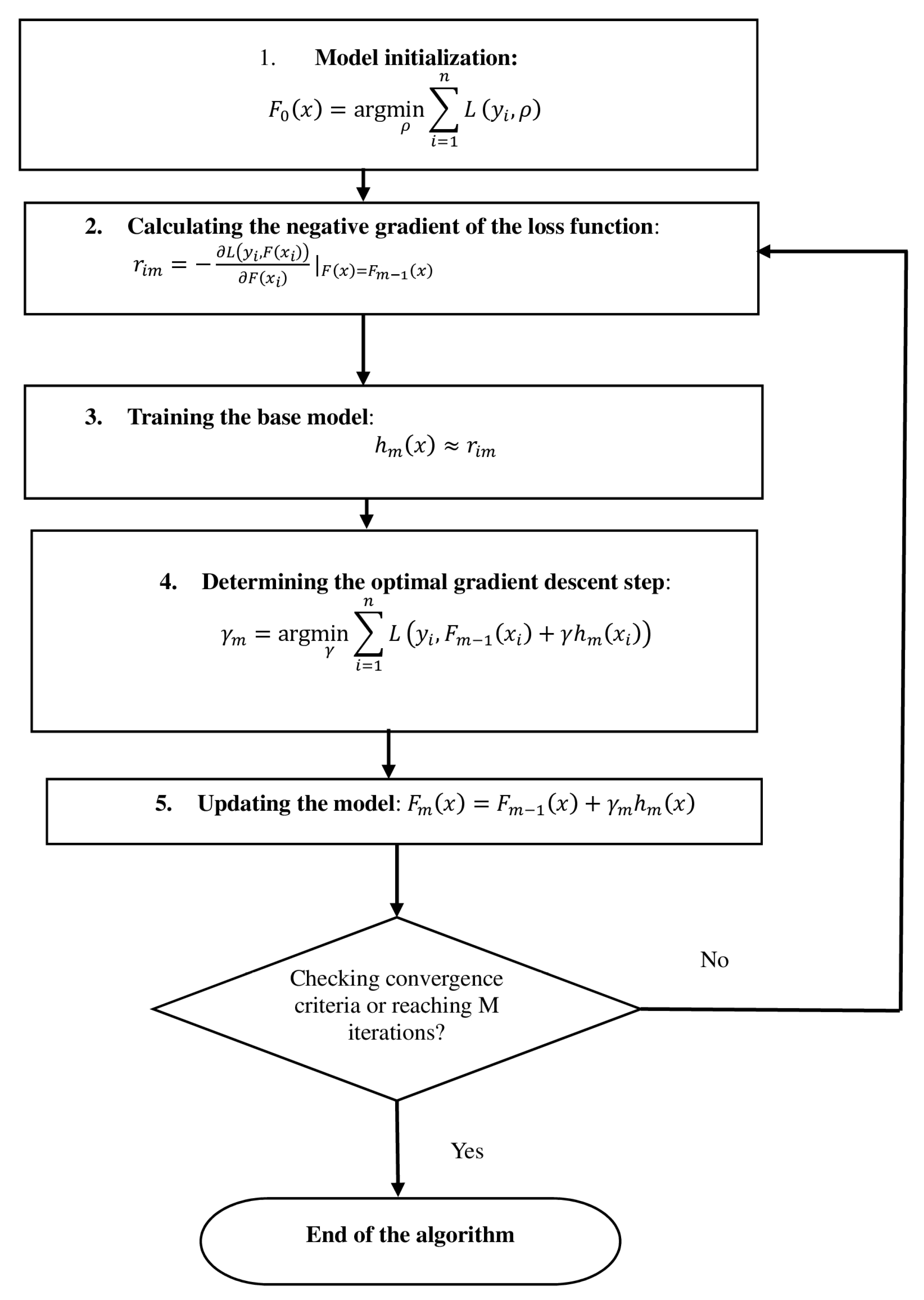
The stages of the algorithm in the context of predicting the CFST column parameters are presented in Figure 3.

Figure 3.
CatBoost algorithm stages.
The training process was carried out for 4000 iterations, which ensured deep model development and minimization of errors on the training dataset. The learning rate was set to 0.01, which allowed us to achieve a balance between the convergence rate and the stability of the process, avoiding sharp fluctuations in error values. The tree depth (the number of nodes on the longest path from the root of the tree to the farthest leaf) was chosen to be equal to 6 to ensure the ability of the model to identify complex relationships between features while minimizing the risk of overfitting.
To assess the quality of the predictions, the root mean square error (RMSE) metric was used, which is standard for regression problems. This metric allows one to quantitatively estimate the average deviation of predicted values from actual ones.
During the training process, training datasets were randomly divided into “Train”, “Validation”, and “Test” samples in the proportion of 70%:15%:15%.
3. Results and Discussion
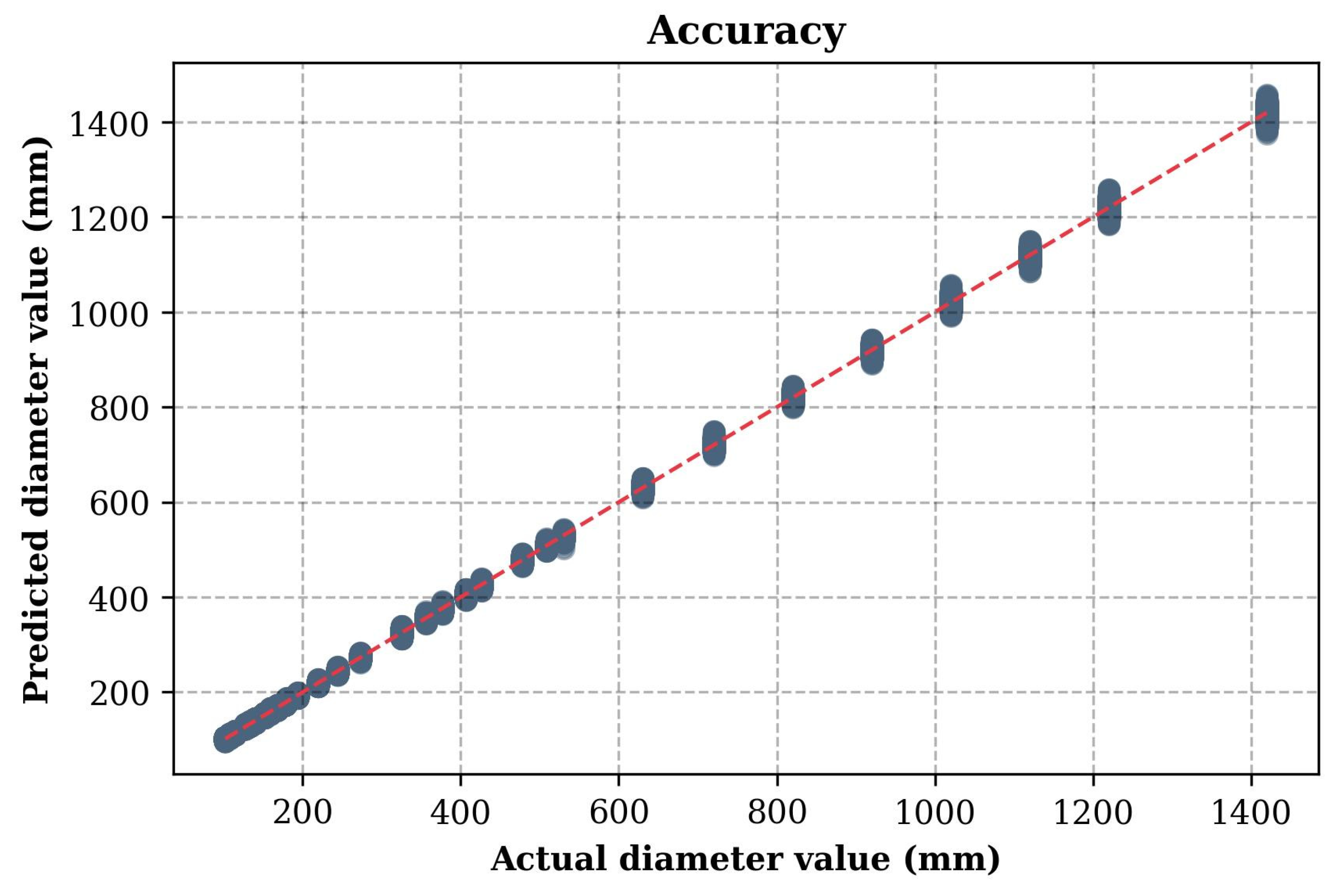
As a result of testing the first model which predicts the cross-section diameter at minimum wall thickness, the RMSE value obtained was 3.86. This indicates that the average deviation of the CFST columns predicted diameters from the actual values at the level of 3.86 mm. This result can be considered satisfactory, which confirms the effectiveness of the CatBoost model in identifying dependencies between input parameters and target values.
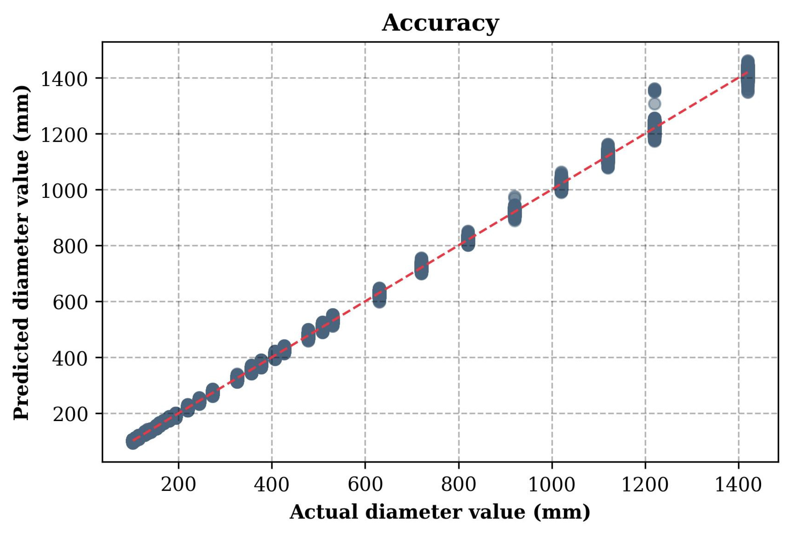
Figure 4 shows a graph illustrating the accuracy of the model predictions, comparing the actual and predicted values. The X-axis shows the actual values of the target variable (the diameter of the CFST columns from the test dataset), and the Y-axis shows the corresponding predicted values. Each point on the graph corresponds to one sample from the test set. The red diagonal line, described by the equation Y = X, represents the perfect match between the predictions and the actual values. The closer the points are to this line, the higher the accuracy of the model.
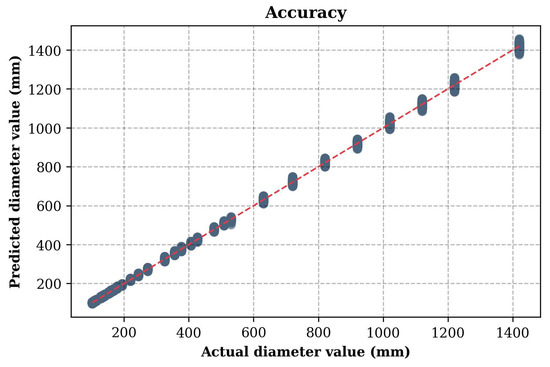
Figure 4.
Comparison of actual and predicted values for the first model predicting the cross-section diameter at minimum wall thickness.
The graph analysis shows that most of the points are in close proximity to the red line, indicating high prediction accuracy. The minimal scatter of the points, especially in the low and medium range, confirms the stability of the model. Minor deviations are observed in the high value range, which may be due to insufficient training data in this range or increased prediction complexity. Overall, the CatBoost model demonstrates high performance in predicting the diameter of CFST columns, and small deviations can be eliminated by additional training or increasing the volume of data or optimizing hyperparameters.
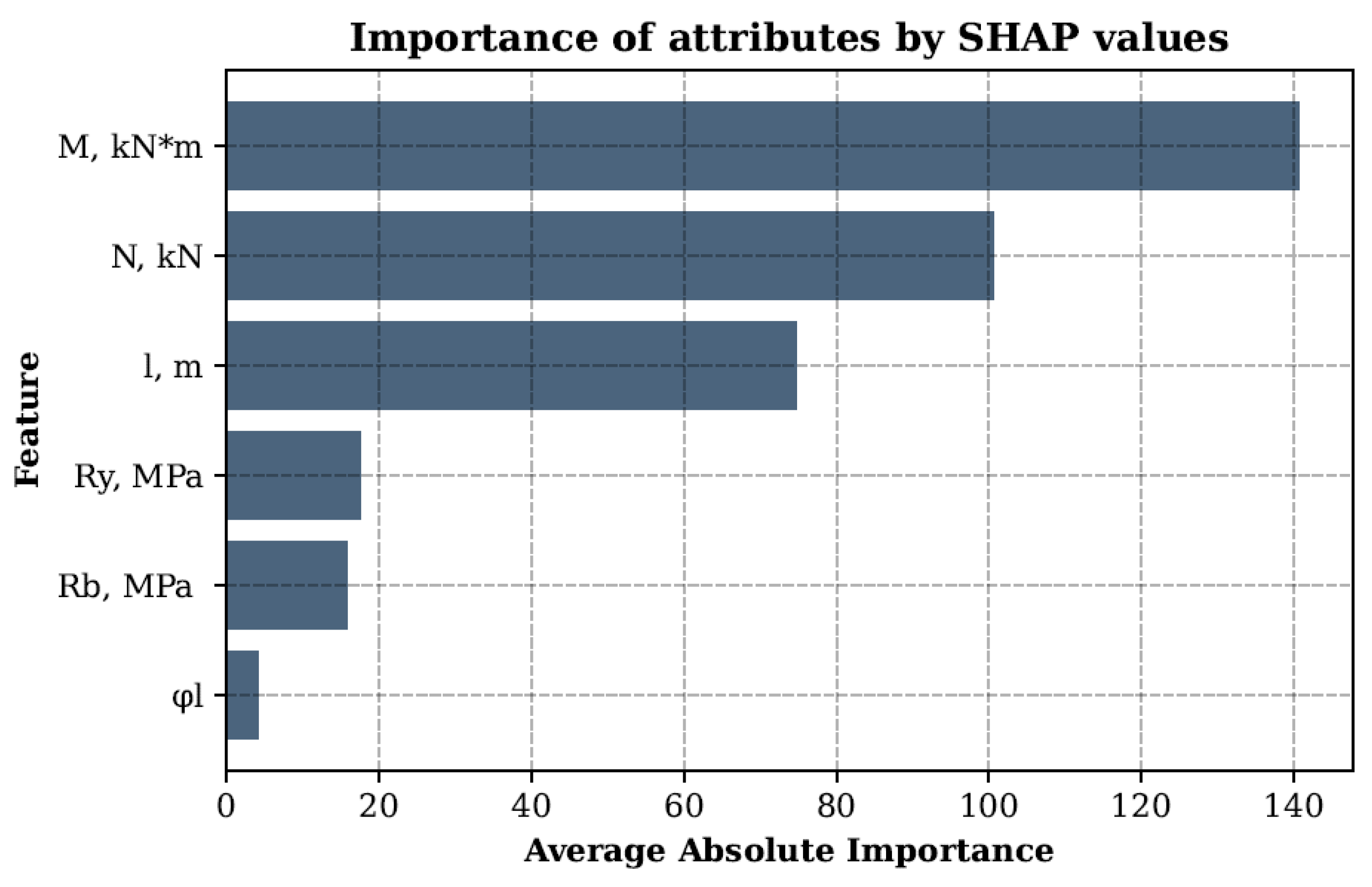
In order to assess the significance of input features for the model, SHAP values were used, which allowed us to interpret the contribution of each feature to the final prediction.
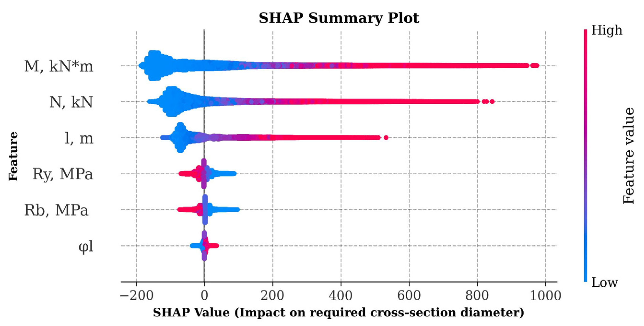
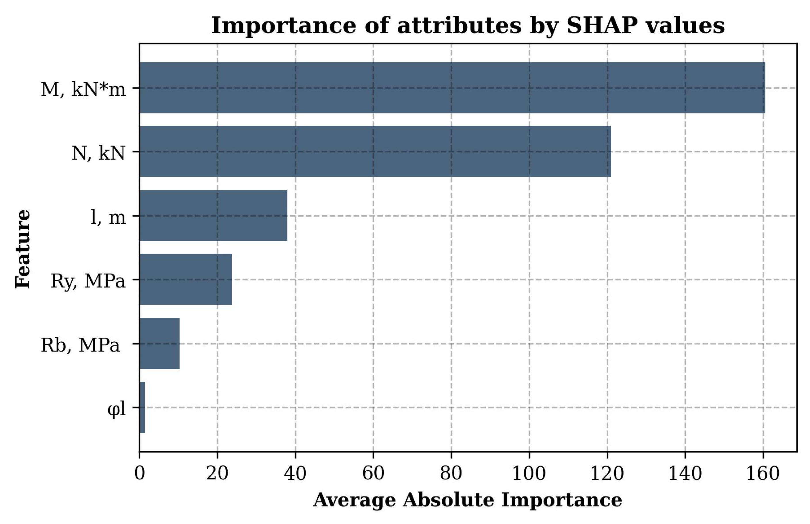
The graph in Figure 5 shows the average absolute SHAP values for each feature, allowing us to identify the main factors influencing the prediction of the cross-sectional diameter. Based on the graph analysis, it can be concluded that the greatest influence on the model was exerted by the design bending moment with an average absolute importance SHAP value of 140.64, followed by the compressive axial force (100.63). The design column length also had a significant influence (74.78), while the yield strength of steel (17.53), the design strength of concrete (15.59), and the share of long-term loads (4.15) were less significant. The SHAP value distribution graph in Figure 6 demonstrates the relationship between the feature values and their influence on the model output: higher feature values for and positively bias the prediction, while values with less importance, such as , have virtually no effect. In general, the conducted analysis confirms the key role of the internal force calculated values in predicting the required geometric parameters of CFST columns, which corresponds to engineering logic and the requirements of regulatory documents. The smaller influence of the materials’ strength characteristics can be explained by their smaller spread in the training dataset compared to the values , , and l.

Figure 5.
Average absolute importance of features for the first model predicting the cross-section diameter at minimum wall thickness.

Figure 6.
Effect of features on the prediction of cross-section diameter at minimum wall thickness using SHAP values.
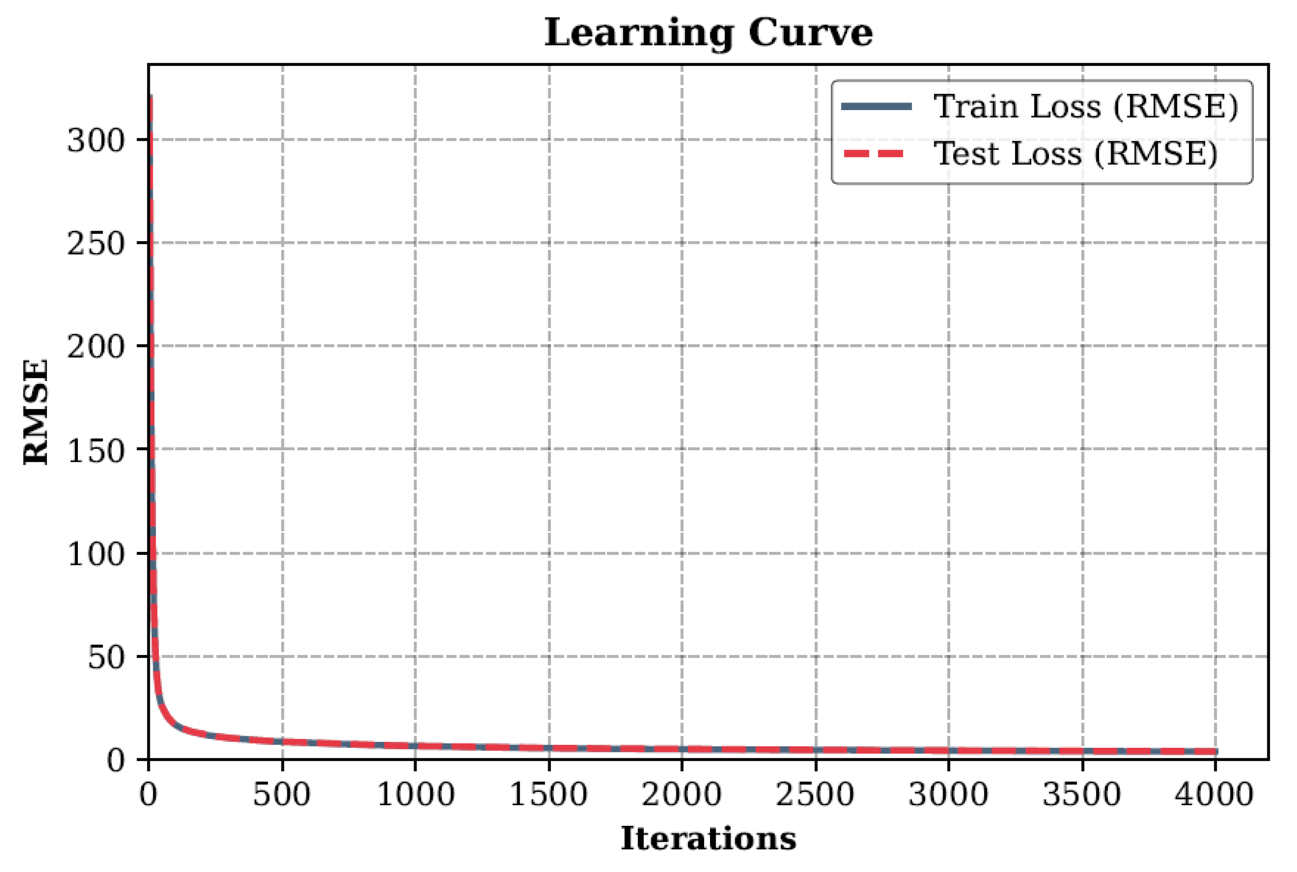
The graph of the loss function, presented in Figure 7, demonstrates the convergence process of the first model during training. At the initial moment of the iteration process, the root mean square error (RMSE) reaches values of about 320, which indicates a significant initial discrepancy between the predicted values and the real data. In the first 100–200 iterations, a sharp decrease in RMSE to a level of less than 50 is observed, which indicates rapid adaptation of the model to the original data.
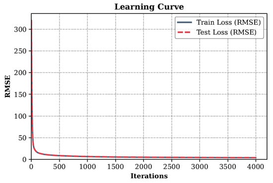
Figure 7.
Loss function (RMSE) during the training of the first model predicting the cross-section diameter at minimum wall thickness.
After 500 iterations, the error decreases to values less than 10, and further training is accompanied by a smoother decrease in RMSE. Upon reaching 1000 iterations, the error value stabilizes in the range of 2–3, which indicates that the model has reached a plateau. In subsequent iterations, up to 4000, the error changes are insignificant, which indicates the absence of overtraining and sufficient convergence of the model.
Despite the high accuracy of the second model’s predictions (Figure 8), small deviations at large diameter values indicate the possibility of further improvement. In order to improve the quality of forecasting, conducting a deeper optimization of hyperparameters and also considering the use of ensemble and regularization methods to improve the generalizing ability of the model and reduce overfitting are recommended.
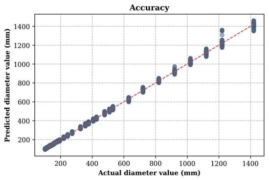
Figure 8.
Comparison of actual and predicted values for the second model predicting the cross-section diameter at maximum wall thickness.
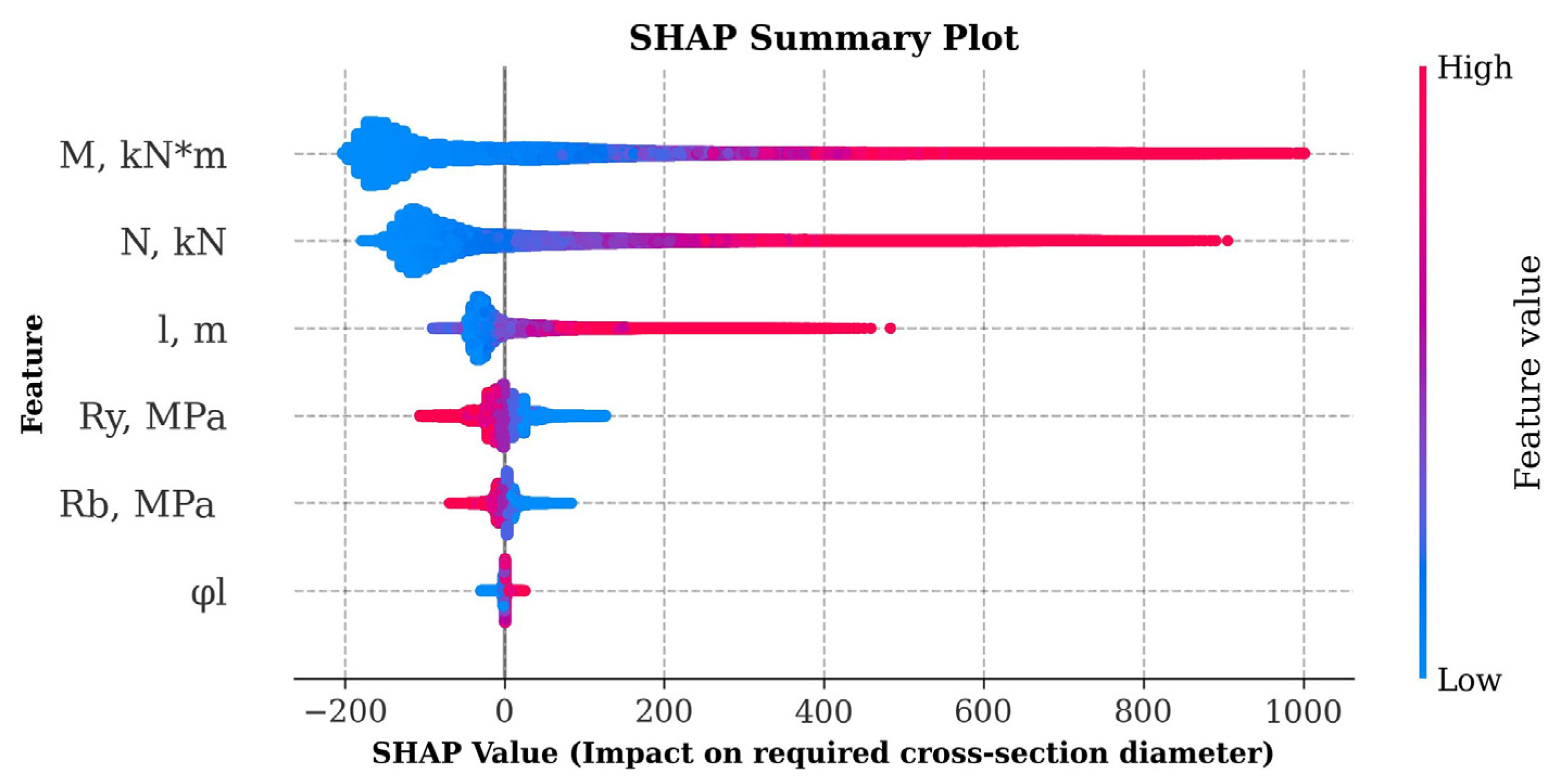
The graph in Figure 9 illustrates the importance of such features as bending moment (M) and axial force (N), which is due to their direct effect on the stress state of the structure. The length of the element (l) also affects the result, but to a much lesser extent, while the yield strength of steel (Ry), the strength of concrete (Rb), and the share of long-term load (φl) play a secondary role. This indicates the predominant importance of force and geometric characteristics over material parameters in the context of the problem under consideration.
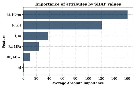
Figure 9.
Average absolute importance of features for the second model predicting the cross-section diameter at maximum wall thickness.
The graph in Figure 10 shows how the direction and magnitude of each feature affect the predictions. High values of M and N significantly increase the predicted diameter, which is consistent with the physical nature of the process: with increasing bending moments and axial forces, the required size of the column cross-section increases. Increasing the length of the structure moderately increases the predicted diameter values, while changes in material properties have little effect, probably due to their lower variability in the training dataset. The long-term load share coefficient has virtually no effect on the result, which allows us to consider excluding it without degrading the prediction quality.

Figure 10.
Effect of features on the prediction of cross-section diameter at maximum wall thickness using SHAP values.
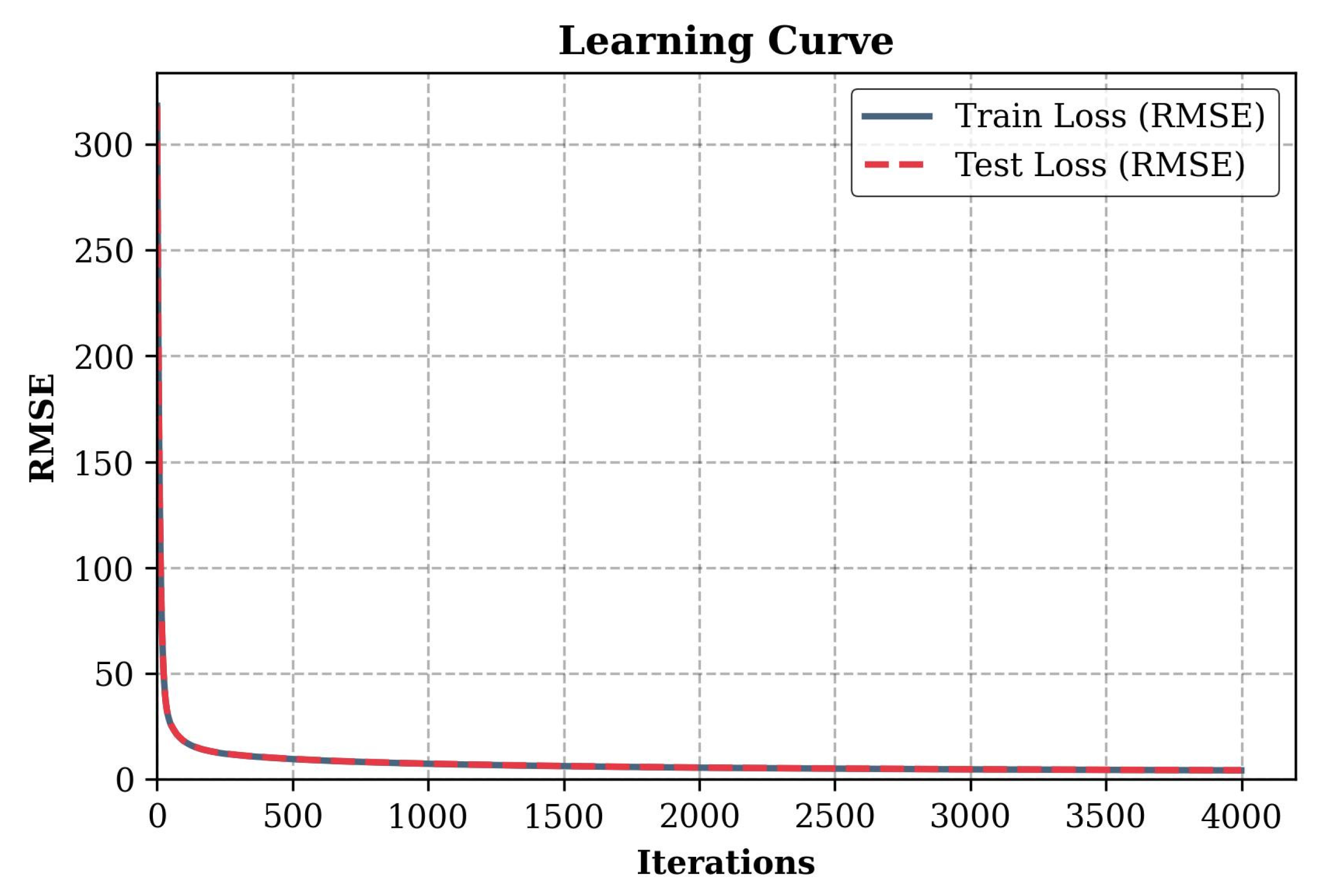
The loss function plot shown in Figure 11 demonstrates the convergence process of the second CatBoost model during training. At the initial moment, the root mean square error (RMSE) exceeds 300, after which, in the first 100–200 iterations, it quickly decreases below 50, which indicates a high speed of adaptation of the model to the data.
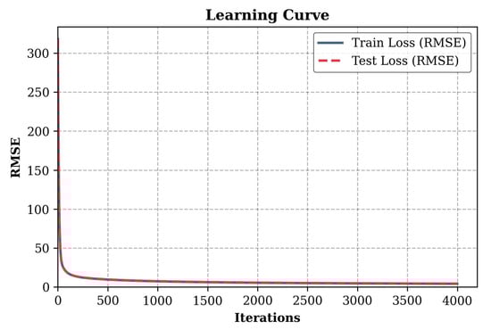
Figure 11.
Loss function (RMSE) during the training of the second model predicting the cross-section diameter at maximum wall thickness.
After 500 iterations, the RMSE reaches about 10, and by the 1000th iteration, it approaches 2–3, and then the error values stabilize, which confirms that the model has reached a stable state.
Comparison with the loss function graph for the first model predicting the cross-section diameter at minimum wall thickness (Figure 7) shows similar learning dynamics, which confirms the stability of the method. The final RMSE value for the second model predicting the required diameter at maximum wall thickness was 4.12 mm, which is close to the result for the first model. Minor differences in the convergence rate and the final error level may be due to hyperparameter settings or data features, which is of interest for further analysis.
The third model was designed to predict the wall thickness of CFST columns (tₚ) using a set of input parameters: axial force (N, kN), bending moment (M, kN∙m), yield strength of steel (Ry, MPa), design strength of concrete (Rb, MPa), column length (l, m), and coefficient φl and outer diameter of the column (Dp, mm). The target variable is the pipe wall thickness (tp, mm). For the third model, predicting the wall thickness of CFST columns, the CatBoost algorithm was initially used. However, as the results showed, CatBoost demonstrated insufficient accuracy for thickness values over 25 mm, which was expressed in a significant dispersion of predicted points relative to the actual wall thickness values of CFST columns. This deviation, when comparing predicted and actual data, was especially pronounced in the area of high loads and large thicknesses, where the model was unable to provide sufficient accuracy. The insufficient accuracy of CatBoost for thickness values over 25 mm could be associated with the limitations of the algorithm itself in processing complex nonlinear dependencies, especially under conditions of high loads and significant thicknesses.
To improve accuracy, a two-layer artificial neural network model with 16 neurons on each hidden layer was built and the Levenberg–Marquardt algorithm was applied to train it. The TANSIG (hyperbolic tangent) function was used as the activation function of the hidden layer neurons. This approach improved the quality of forecasting, especially in the area of significant wall thickness, which confirmed its applicability for solving engineering problems with high accuracy.
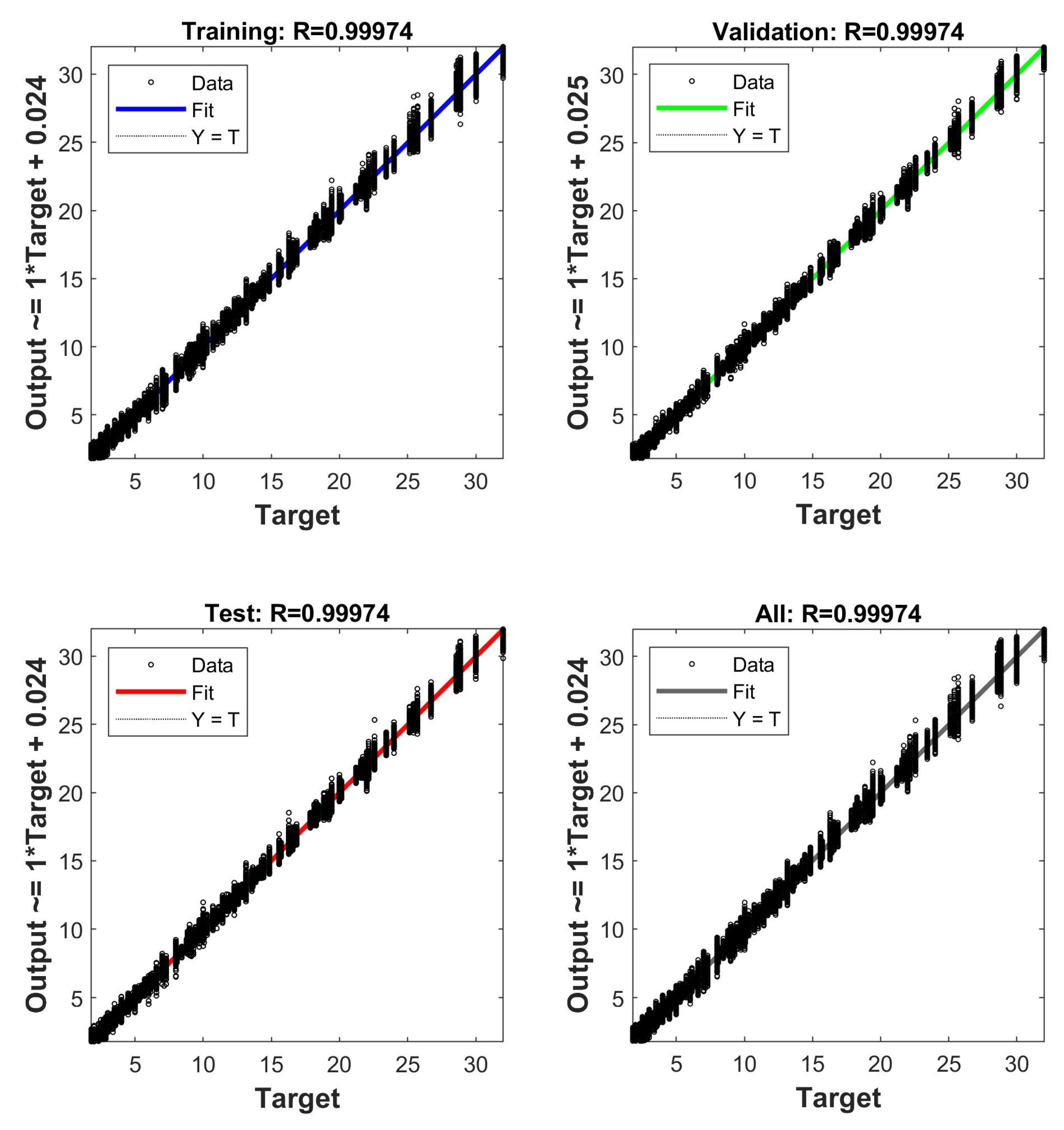
The results of the artificial neural network model implemented in MATLAB are confirmed by the graphs in Figure 12. The model demonstrates exceptionally high accuracy at all stages, including training, validation, testing, and the general dataset. The correlation coefficient R = 0.99974 on the training, validation, and testing samples and the general dataset indicates an almost perfect match between the predicted and real values. The graphs show that the approximating line (Fit) almost completely coincides with the ideal line Y = T, and the points on the graph are tightly grouped around it. This indicates a high generalizing ability of the model, the absence of overfitting, and the correct choice of hyperparameters.

Figure 12.
Evaluation of the neural network model training quality.
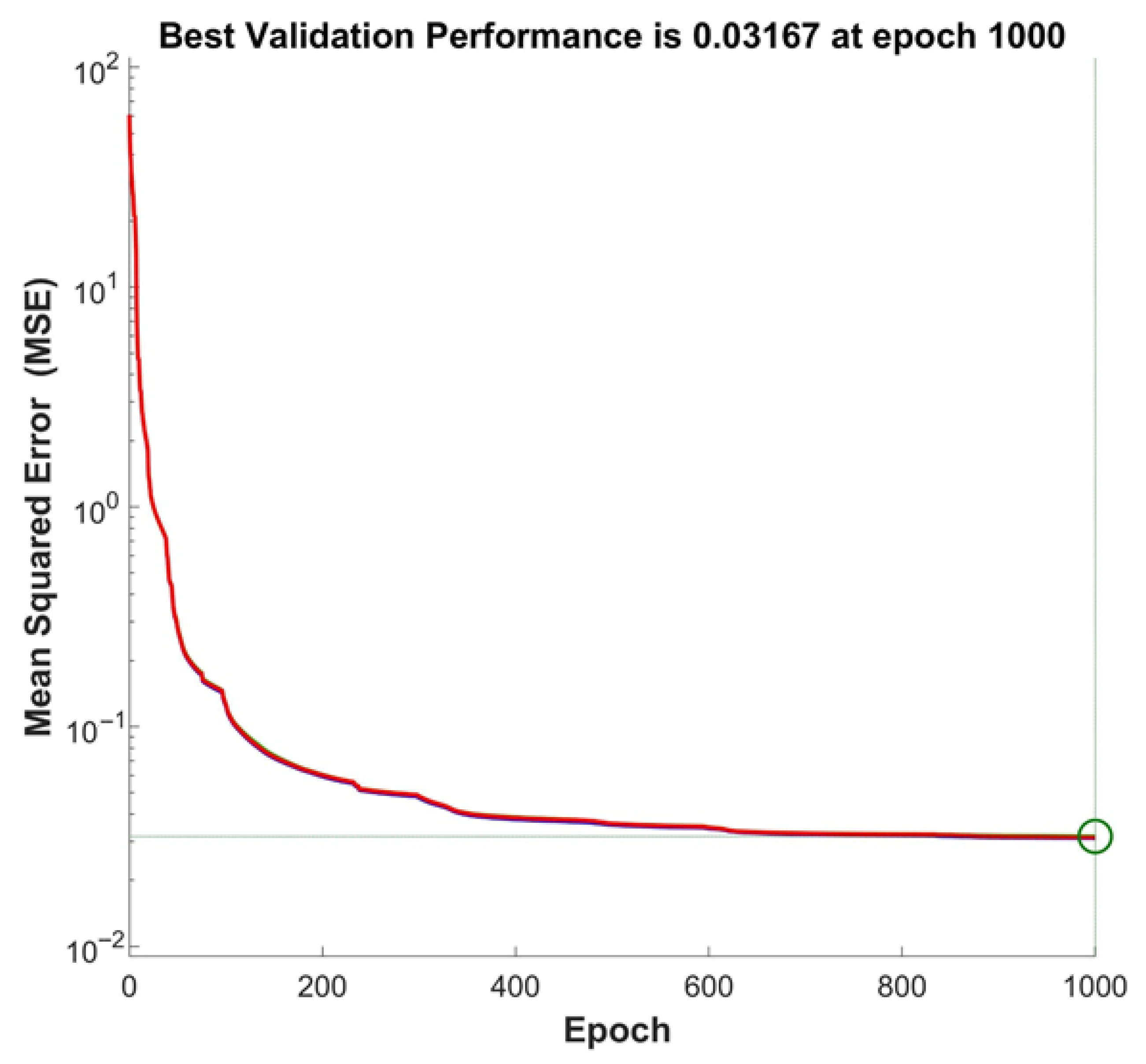
To assess the efficiency of the model training process, an analysis of the change in the mean square error (MSE) dynamics of the model was carried out. Figure 13 shows the dynamics of the change in the mean square error during training the model on the third dataset for predicting the wall thickness of CFST columns.

Figure 13.
Dynamics of change in the mean square error (MSE) during training of the neural network on the third dataset for predicting the wall thickness of CFST columns.
The curve shows that the error is significantly reduced already at the initial stages of training, which indicates rapid convergence of the model. As the number of epochs (full passes over the entire training dataset) increases, the rate of decrease in MSE slows down, which is typical for high-accuracy learning processes. The best error value on the validation data was 0.03167, and this was achieved at the 1000th epoch, which confirms the effectiveness of the Levenberg–Marquardt algorithm and the chosen model architecture.
This graph clearly illustrates that the model is successfully trained, achieving a low prediction error, which confirms its applicability to solving the problem of determining the wall thickness of CFST columns.
4. Conclusions
- In this study, three machine learning models were developed to predict the required dimensions of the CFST columns’ cross-section under the combined action of bending moments and compressive axial forces. The first and second models are based on the CatBoost algorithm. They demonstrated high accuracy in predicting the column diameter at the minimum and maximum wall thickness, respectively. The root mean square error (RMSE) for the first model was 3.86 mm, and for the second it was 4.12 mm, which confirms the effectiveness of CatBoost in solving the design problems for CFST columns. The feature importance analysis using SHAP values showed that the bending moment and axial force have the greatest influence on the cross-section outer diameter, which is consistent with the physical nature of the problem.
- The third model, designed to predict the pipe wall thickness of CFST columns, was initially implemented using CatBoost. However, at thickness values over 25 mm, a significant dispersion of predicted points was observed, indicating insufficient accuracy of the model in the area of high loads and large thicknesses. To improve accuracy, an artificial neural network model was built and the Levenberg–Marquardt training algorithm was applied, which successfully coped with the task, ensuring an almost perfect match between the predicted and actual values (correlation coefficient R = 0.99974). The training and testing graphs confirmed the high generalizing ability of the model, the absence of overtraining, and the stability of the operation at all stages.
- The results of this study showed that the use of machine learning methods such as CatBoost and the Levenberg–Marquardt algorithm allows for an efficient solution of CFST column design problems by automating the process of determining the section geometric parameters. This is especially important in the context of restrictions imposed by national standards and the need to take into account complex nonlinear dependencies between input parameters. The proposed models can operate with concrete compressive strength from 10 to 65 MPa and steel yield strength from 240 to 440 MPa over the entire possible range of the calculated column lengths.
- Considering the successful application of the developed models for circular sections, it is possible in the future to adapt the proposed algorithms for predicting the geometric parameters of rectangular CFST columns. Further research may also be directed towards implementing similar machine learning models using design codes from other countries, such as ACI318, AISC360-16, Eurocode 4, CEB-FIP Model Code 90, etc.
- Currently, the determination of CFST column cross-section dimensions is performed by a simple manual selection of options, or the dimensions are assigned based on design experience with subsequent verification of the strength condition. This approach may require trying a large number of options to obtain the optimal solution. The models we have developed have been trained on over a million samples and do this job much more efficiently than an experienced designer. The developed models can be integrated into computer-aided design (CAD) systems and finite element analysis (FEA) software packages as extensions. This will not only speed up the design process of CFST columns but also improve the accuracy of calculations, providing more reliable and cost-effective solutions for building structures.
Author Contributions
Conceptualization, A.C. and S.A.-Z.; methodology, A.C. and S.A.-Z.; software, V.T. and S.A.-Z.; validation, A.C. and S.A.-Z.; formal analysis, A.C.; investigation, S.A.-Z.; resources, S.A.-Z.; data curation, V.T.; writing—original draft preparation, A.C. and S.A.-Z.; writing—review and editing, V.T.; visualization, A.C.; supervision, A.C.; project administration, A.C.; funding acquisition, A.C. All authors have read and agreed to the published version of the manuscript.
Funding
The APC was funded by Don State Technical University.
Data Availability Statement
Training datasets, developed programs for generating training datasets, and trained machine learning models are available for download at the following link: https://disk.yandex.ru/d/5oLeUktAkFpyyg, accessed on 14 April 2025.
Acknowledgments
The authors would like to acknowledge the administration of Don State Technical University for their resources and financial support.
Conflicts of Interest
The authors declare no conflicts of interest. The funders had no role in the design of the study; in the collection, analyses, or interpretation of the data; in the writing of the manuscript; or in the decision to publish the results.
Abbreviations
The following notations are used in this manuscript:
| N | Axial force |
| M | Bending moment |
| Ry | Yield strength of steel |
| Rb | Concrete compressive strength |
| l | Calculated length of the column |
| Coefficient that takes into account the share of long-term loads in the total load | |
| Bending moment from the action of the full load | |
| Bending moment from the action of constant and long-term loads | |
| Eccentricity of the axial force | |
| Ultimate bending moment | |
| Internal radius of the steel pipe | |
| Cross-sectional area of the steel shell | |
| Thickness of the steel pipe | |
| Radius of the steel shell middle surface | |
| Calculated strength of concrete under compression as part of a CFST element | |
| Calculated strength of steel under compression as part of a CFST element | |
| Angle determining the position of the concrete compressed zone in the ultimate state | |
| Increase in compressive strength of concrete due to work in confined conditions | |
| m | Coefficient that takes into account the influence of eccentricity when calculating the value |
| c | Empirical constant equal to 25 MN |
| Calculated eccentricity without taking into account the deflection of the element | |
| Random eccentricity | |
| Euler critical force | |
| Coefficient that takes into account the additional eccentricity caused by deflection | |
| Reduced bending stiffness of the cross-section | |
| Coefficient that reduces the stiffness of the section due to the plastic work of concrete | |
| Long-term concrete modulus of deformation | |
| Moment of inertia for the concrete part of the composite section | |
| Coefficient that reduces the stiffness of the section due to the plastic work of steel | |
| Moment of inertia for the steel shell | |
| Modulus of elasticity of steel | |
| Initial modulus of elasticity of concrete | |
| Creep coefficient of concrete | |
| Relative axial force eccentricity | |
| Ultimate axial force under central compression | |
| Ultimate bending moment for pure bending | |
| Dp1 | Cross-sectional diameter predicted by model 1 (at minimum wall thickness) |
| Dp2 | Cross-sectional diameter predicted by model 2 (at maximum wall thickness) |
| D | Training sample |
| Vector of features describing the structural and load characteristics of the column | |
| Target variable corresponding to the predicted parameter | |
| Number of observations in the sample | |
| Number of features | |
| Approximating function | |
| Loss function | |
| Initial prediction | |
| Weak model at the m-th step, trained on the mistakes of previous models | |
| Learning coefficient |
References
- Han, L.H.; Li, W.; Bjorhovde, R. Developments and advanced applications of concrete-filled steel tubular (CFST) structures: Members. J. Constr. Steel Res. 2014, 100, 211–228. [Google Scholar] [CrossRef]
- Chen, Z.; Gao, F.; Hu, J.; Liang, H.; Huang, S. Creep and shrinkage monitoring and modelling of CFST columns in a super high-rise under-construction building. J. Build. Eng. 2023, 76, 107282. [Google Scholar] [CrossRef]
- Tran, H.; Thai, H.T.; Ngo, T.; Uy, B.; Li, D.; Mo, J. Nonlinear inelastic simulation of high-rise buildings with innovative composite coupling shear walls and CFST columns. Struct. Des. Tall Spec. Build. 2021, 30, e1883. [Google Scholar] [CrossRef]
- Nguyen, T.T.; Thai, H.T.; Li, D.; Wang, J.; Uy, B.; Ngo, T. Behaviour and design of eccentrically loaded CFST columns with high strength materials and slender sections. J. Constr. Steel Res. 2022, 188, 107004. [Google Scholar] [CrossRef]
- Xiang, N.; Feng, Y.; Chen, X. Novel fiber-based seismic response modelling and design method of partially CFST bridge piers considering local buckling effect. Soil Dyn. Earthq. Eng. 2023, 170, 107911. [Google Scholar] [CrossRef]
- Wang, C.; Li, H.; Xu, L.; Xu, K.; Zhao, L.; Chen, Q. Seismic performance of PS-CFST bridge piers with novel external replaceable energy dissipating devices. J. Constr. Steel Res. 2025, 224, 109156. [Google Scholar] [CrossRef]
- Ji, S.H.; Wang, W.D.; Chen, W.; Xian, W.; Wang, R.; Shi, Y.L. Experimental and numerical investigation on the lateral impact responses of CFST members after exposure to fire. Thin-Walled Struct. 2023, 190, 110968. [Google Scholar] [CrossRef]
- Thai, H.T.; Thai, S.; Ngo, T.; Uy, B.; Kang, W.H.; Hicks, S.J. Reliability considerations of modern design codes for CFST columns. J. Constr. Steel Res. 2021, 177, 106482. [Google Scholar] [CrossRef]
- İpek, S.; Güneyisi, E.M. Nonlinear finite element analysis of double skin composite columns subjected to axial loading. Arch. Civ. Mech. Eng. 2020, 20, 9. [Google Scholar] [CrossRef]
- Ilanthalir, A.; Regin, J.J.; Maheswaran, J. Concrete-filled steel tube columns of different cross-sectional shapes under axial compression: A review. IOP Conf. Ser. Mater. Sci. Eng. 2020, 983, 012007. [Google Scholar] [CrossRef]
- Bhatia, S.; Tiwary, A.K. Axial Compression Behavior of Single-Skin and Double-Skin Concrete-Filled Steel Tube Columns: A Review. Lect. Notes Civ. Eng. 2022, 196, 849–861. [Google Scholar] [CrossRef]
- Yang, C.; Gao, P.; Wu, X.; Chen, Y.F.; Li, Q.; Li, Z. Practical formula for predicting axial strength of circular-CFST columns considering size effect. J. Constr. Steel Res. 2020, 168, 105979. [Google Scholar] [CrossRef]
- Erdoğan, A.; Güneyisi, E.M.; İpek, S. Finite Element Modelling of Ultimate Strength of CFST Column and Its Comparison with Design Codes. Bilecik Şeyh Edebali Univ. J. Sci. 2022, 9, 324–339. [Google Scholar] [CrossRef]
- Ding, F.; Cao, Z.; Lyu, F.; Huang, S.; Hu, M.; Lin, Q. Practical design equations of the axial compressive capacity of circular CFST stub columns based on finite element model analysis incorporating constitutive models for high-strength materials. Case Stud. Constr. Mater. 2022, 16, e01115. [Google Scholar] [CrossRef]
- Nguyen, D.H.; Hong, W.K.; Ko, H.J.; Kim, S.K. Finite element model for the interface between steel and concrete of CFST (concrete-filled steel tube). Eng. Struct. 2019, 185, 141–158. [Google Scholar] [CrossRef]
- Gao, H. Calculation of Load-Carrying Capacity of Square Concrete Filled Tube Columns Based on Neural Network. Appl. Mech. Mater. 2011, 351–352, 713–716. [Google Scholar] [CrossRef]
- Wang, H.J.; Zhu, H.B.; Wei, H. Bearing capacity of concrete filled square steel tubular columns based on neural network. Adv. Mater. Res. 2012, 502, 193–197. [Google Scholar] [CrossRef]
- Wei, H.; Du, Y.; Wang, H.J. Seismic behavior of concrete filled circular steel tubular columns based on artificial neural network. Adv. Mater. Res. 2012, 502, 189–192. [Google Scholar] [CrossRef]
- Ahmadi, M.; Naderpour, H.; Kheyroddin, A. Utilization of artificial neural networks to prediction of the capacity of CCFT short columns subject to short term axial load. Arch. Civ. Mech. Eng. 2014, 14, 510–517. [Google Scholar] [CrossRef]
- Du, Y.; Chen, Z.; Zhang, C.; Cao, X. Research on axial bearing capacity of rectangular concrete-filled steel tubular columns based on artificial neural networks. Front. Comput. Sci. 2017, 11, 863–873. [Google Scholar] [CrossRef]
- Le, T.T.; Asteris, P.G.; Lemonis, M.E. Prediction of axial load capacity of rectangular concrete-filled steel tube columns using machine learning techniques. Eng. Comput. 2022, 38, 3283–3316. [Google Scholar] [CrossRef]
- Zarringol, M.; Thai, H.T. Prediction of the load-shortening curve of CFST columns using ANN-based models. J. Build. Eng. 2022, 51, 104279. [Google Scholar] [CrossRef]
- Đorđević, F.; Kostić, S.M. Practical ANN prediction models for the axial capacity of square CFST columns. J. Big Data 2023, 10, 67. [Google Scholar] [CrossRef]
- Tran, V.L.; Jang, Y.; Kim, S.E. Improving the axial compression capacity prediction of elliptical CFST columns using a hybrid ANN-IP model. Steel Compos. Struct. 2021, 39, 319–335. [Google Scholar] [CrossRef]
- Bardhan, A.; Biswas, R.; Kardani, N.; Iqbal, M.; Samui, P.; Singh, M.; Asteris, P.G. A novel integrated approach of augmented grey wolf optimizer and ANN for estimating axial load carrying-capacity of concrete-filled steel tube columns. Constr. Build. Mater. 2022, 337, 127454. [Google Scholar] [CrossRef]
- Nguyen, T.H.; Tran, N.L.; Nguyen, D.D. Prediction of axial compression capacity of cold-formed steel oval hollow section columns using ANN and ANFIS models. Int. J. Steel Struct. 2022, 22, 2018–2027. [Google Scholar] [CrossRef]
- Zarringol, M.; Patel, V.I.; Liang, Q.Q. Artificial neural network model for strength predictions of CFST columns strengthened with CFRP. Eng. Struct. 2023, 281, 115784. [Google Scholar] [CrossRef]
- Tran, V.L.; Thai, D.K.; Nguyen, D.D. Practical artificial neural network tool for predicting the axial compression capacity of circular concrete-filled steel tube columns with ultra-high-strength concrete. Thin-Walled Struct. 2020, 151, 106720. [Google Scholar] [CrossRef]
- Faridmehr, I.; Nehdi, M.L.; Nejad, A.F.; Sahraei, M.A.; Kamyab, H.; Valerievich, K.A. An innovative multi-objective optimization approach for compact concrete-filled steel tubular (CFST) column design utilizing lightweight high-strength concrete. Int. J. Light. Mater. Manuf. 2024, 7, 405–425. [Google Scholar] [CrossRef]
- Naser, M.Z.; Thai, S.; Thai, H.T. Evaluating structural response of concrete-filled steel tubular columns through machine learning. J. Build. Eng. 2021, 34, 101888. [Google Scholar] [CrossRef]
- Nguyen, T.T.; Nguyen, P.C. Improving the Accuracy of ACI 318-08 Design Standard for Predicting Strength of CFST Columns Using Machine Learning. In Proceedings of the 3rd Annual International Conference on Material, Machines and Methods for Sustainable Development (MMMS2022), Can Tho, Vietnam, 10–13 November 2022; pp. 19–25. [Google Scholar] [CrossRef]
- Nguyen, T.; Le Nguyen, K.; Ly, H. Universal boosting ML approaches to predict the ultimate load capacity of CFST columns. Struct. Des. Tall Spec. Build. 2024, 33, e2071. [Google Scholar] [CrossRef]
- Nguyen, T.A.; Nguyen, M.H.; Ly, H.B. Unified machine learning approach for predicting CFST column axial load capacity. Innov. Infrastruct. Solut. 2024, 9, 295. [Google Scholar] [CrossRef]
- Lai, D.; Wei, J.; Contento, A.; Xue, J.; Briseghella, B.; Albanesi, T.; Demartino, C. Machine learning-based probabilistic predictions for Concrete Filled Steel Tube (CFST) column axial capacity. Structures 2024, 70, 107543. [Google Scholar] [CrossRef]
- Li, J.; Pang, Y.; Mu, Q.; Zhang, X.; Shi, Y.; Wang, H. Post-blast capacity evaluation of concrete-filled steel tubular (CFST) column based on machine learning technique. Adv. Struct. Eng. 2023, 26, 1953–1972. [Google Scholar] [CrossRef]
- He, J.; Jiang, L.; Jiang, L.; Wen, T.; Hu, Y.; Guo, W.; Sun, J. Estimation of blast-induced peak response of concrete-filled double-skin tube columns by intelligence-based technique. Thin-Walled Struct. 2023, 186, 110670. [Google Scholar] [CrossRef]
- Momeni, M.; Hadianfard, M.A.; Bedon, C.; Baghlani, A. Damage evaluation of H-section steel columns under impulsive blast loads via gene expression programming. Eng. Struct. 2020, 219, 110909. [Google Scholar] [CrossRef]
- Zarringol, M.; Naser, M.Z. Explainable machine learning model for prediction of axial capacity of strengthened CFST columns. In Interpretable Machine Learning for the Analysis, Design, Assessment, and Informed Decision Making for Civil Infrastructure; Woodhead Publishing Series in Civil and Structural Engineering; Elsevier: Amsterdam, The Netherlands, 2024; pp. 229–253. [Google Scholar] [CrossRef]
- Nishant Arora, H.C.; Kumar, A.; Kumar, P.; Kapoor, N.R.; Jain, A. Prediction of Axial Capacity of RC Columns Reinforced with Ferro-cement Jacketing: A Data-driven Machine Learning Strategy. KSCE J. Civ. Eng. 2024, 28, 3835–3844. [Google Scholar] [CrossRef]
- Gupta, M.; Prakash, S.; Ghani, S. Enhancing predictive accuracy: A comprehensive study of optimized machine learning models for ultimate load-carrying capacity prediction in SCFST columns. Asian J. Civ. Eng. 2024, 25, 3081–3098. [Google Scholar] [CrossRef]
- Ngo, N.T.; Pham, T.P.T.; Le, H.A.; Nguyen, Q.T.; Nguyen, T.T.N. Axial strength prediction of steel tube confined concrete columns using a hybrid machine learning model. Structures 2022, 36, 765–780. [Google Scholar] [CrossRef]
- Javed, M.F.; Farooq, F.; Memon, S.A.; Akbar, A.; Khan, M.A.; Aslam, F.; Alyousef, R.; Alabduljabbar, H.; Rehman, S.K.U.; Rehman, S.K.U.; et al. New Prediction Model for the Ultimate Axial Capacity of Concrete-Filled Steel Tubes: An Evolutionary Approach. Crystals 2020, 10, 741. [Google Scholar] [CrossRef]
- Sarir, P.; Ruangrassamee, A.; Iwanami, M. Estimation of the axial capacity of high-strength concrete-filled steel tube columns using artificial neural network, random forest, and extreme gradient boosting approaches. Front. Struct. Civ. Eng. 2024, 18, 1794–1814. [Google Scholar] [CrossRef]
- Narang, A.; Kumar, R.; Dhiman, A. Machine learning applications to predict the axial compression capacity of concrete filled steel tubular columns: A systematic review. Multidiscip. Model. Mater. Struct. 2023, 19, 197–225. [Google Scholar] [CrossRef]
- Narang, A.; Kumar, R.; Dhiman, A. Residual strength index prediction of circular concrete-filled steel tubular columns through advanced machine learning methods. Asian J. Civ. Eng. 2024, 25, 747–760. [Google Scholar] [CrossRef]
- Lusong, Y.; Yuxing, Z.; Li, W.; Qiren, P.; Yiyang, W. Prediction of the Axial Bearing Compressive Capacities of CFST Columns Based on Machine Learning Methods. Int. J. Steel Struct. 2024, 24, 81–94. [Google Scholar] [CrossRef]
- Memarzadeh, A.; Sabetifar, H.; Nematzadeh, M. A comprehensive and reliable investigation of axial capacity of Sy-CFST columns using machine learning-based models. Eng. Struct. 2023, 284, 115956. [Google Scholar] [CrossRef]
- Megahed, K.; Mahmoud, N.S.; Abd-Rabou, S.E.M. Application of machine learning models in the capacity prediction of RCFST columns. Sci. Rep. 2023, 13, 24. [Google Scholar] [CrossRef]
- Megahed, K.; Mahmoud, N.; Abd-Rabou, S. Prediction of the axial compression capacity of stub CFST columns using machine learning techniques. Sci. Rep. 2023, 14, 2885. [Google Scholar] [CrossRef]
- Megahed, K. Symbolic regression for strength prediction of eccentrically loaded concrete-filled steel tubular columns. Sci. Rep. 2025, 15, 3085. [Google Scholar] [CrossRef]
- Shen, F.; Jha, I.; Isleem, H.F.; Almoghayer, W.J.K.; Khishe, M.; Elshaarawy, M.K. Advanced predictive machine and deep learning models for round-ended CFST column. Sci. Rep. 2025, 15, 6194. [Google Scholar] [CrossRef]
- Nariman, N.A.; Hamdia, K.; Ramadan, A.M.; Sadaghian, H. Optimum design of flexural strength and stiffness for reinforced concrete beams using machine learning. Appl. Sci. 2021, 11, 8762. [Google Scholar] [CrossRef]
- Tusnin, A.R.; Alekseytsev, A.V.; Tusnina, O. Using Machine Learning Technologies to Design Modular Buildings. Buildings 2024, 14, 2213. [Google Scholar] [CrossRef]
- Lazaridis, P.C.; Kavvadias, I.E.; Demertzis, K.; Iliadis, L.; Vasiliadis, L.K. Interpretable machine learning for assessing the cumulative damage of a reinforced concrete frame induced by seismic sequences. Sustainability 2023, 15, 12768. [Google Scholar] [CrossRef]
- Chepurnenko, A.S.; Turina, V.S.; Akopyan, V.F. Artificial Intelligence Model for Predicting the Load-Bearing Capacity of Eccentrically Compressed Short Concrete Filled Steel Tubular Columns. Constr. Mater. Prod. 2024, 7, 2. [Google Scholar] [CrossRef]
- Nesvetaev, G.V.; Yulia, K.; Shut, V.V. Specific heat dissipation of concrete and the risk of early cracking of massive reinforced concrete foundation slabs. Constr. Mater. Prod. 2024, 7, 3. [Google Scholar] [CrossRef]
- Choi, R.Y.; Coyner, A.S.; Kalpathy-Cramer, J.; Chiang, M.F.; Campbell, J.P. Introduction to machine learning, neural networks, and deep learning. Transl. Vis. Sci. Technol. 2020, 9, 14. [Google Scholar]
- Dorogush, A.V.; Ershov, V.; Gulin, A. CatBoost: Gradient boosting with categorical features support. arXiv 2018, arXiv:1810.11363. [Google Scholar] [CrossRef]
- Levenberg, K. A method for the solution of certain non-linear problems in least squares. Q. Appl. Math. 1944, 2, 164–168. [Google Scholar] [CrossRef]
- Marquardt, D.W. An algorithm for least-squares estimation of nonlinear parameters. J. Soc. Ind. Appl. Math. 1963, 11, 431–441. [Google Scholar] [CrossRef]
- Kaggle: Your Machine Learning and Data Science Community. Available online: https://www.kaggle.com/ (accessed on 5 April 2025).
- Deep Learning Toolbox. Available online: https://www.mathworks.com/help/deeplearning/index.html (accessed on 5 April 2025).
Disclaimer/Publisher’s Note: The statements, opinions and data contained in all publications are solely those of the individual author(s) and contributor(s) and not of MDPI and/or the editor(s). MDPI and/or the editor(s) disclaim responsibility for any injury to people or property resulting from any ideas, methods, instructions or products referred to in the content. |
© 2025 by the authors. Licensee MDPI, Basel, Switzerland. This article is an open access article distributed under the terms and conditions of the Creative Commons Attribution (CC BY) license (https://creativecommons.org/licenses/by/4.0/).