
Seismic Response of Variable Section Column with a Change in Its Boundary Conditions

 ,
,  , and
, and
Abstract
1. Introduction
2. Essential Parameters of the Analytical Method
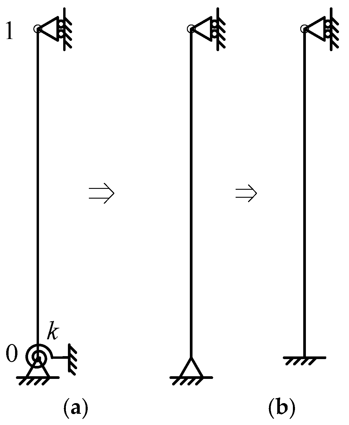
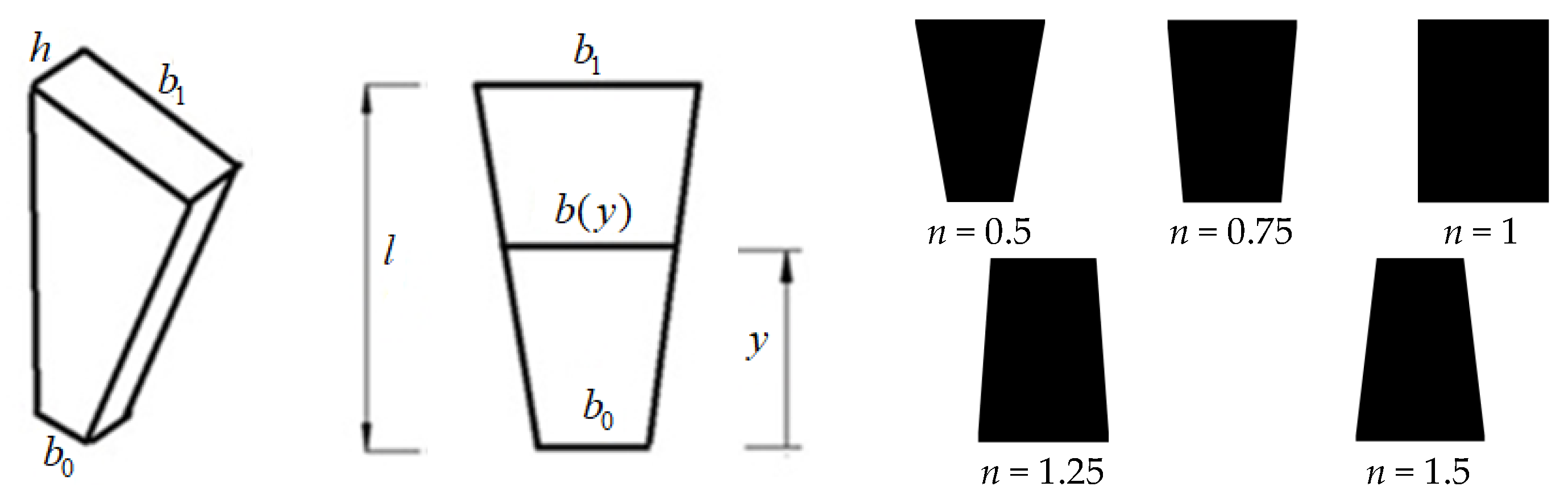
3. Problem Definition
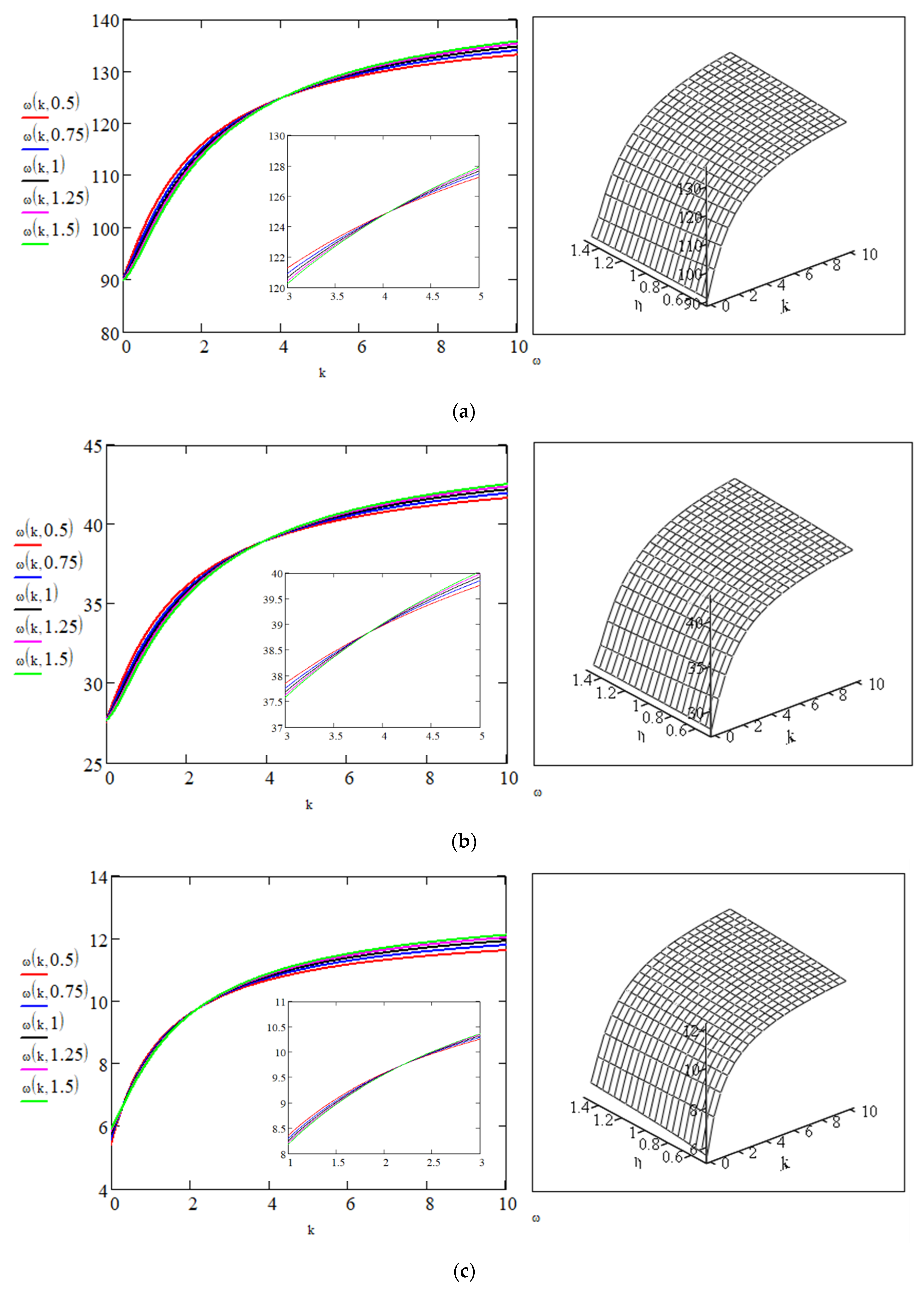
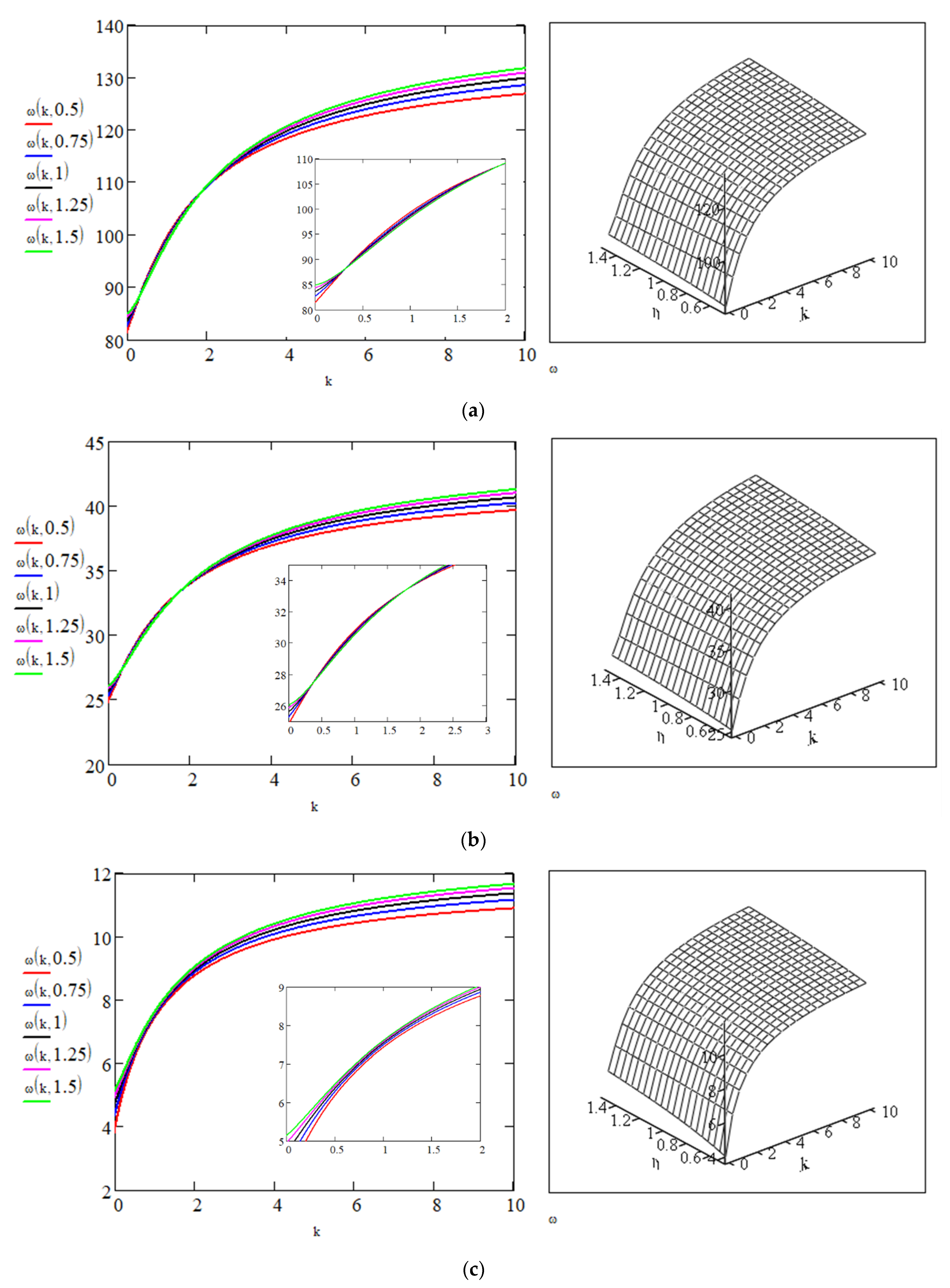
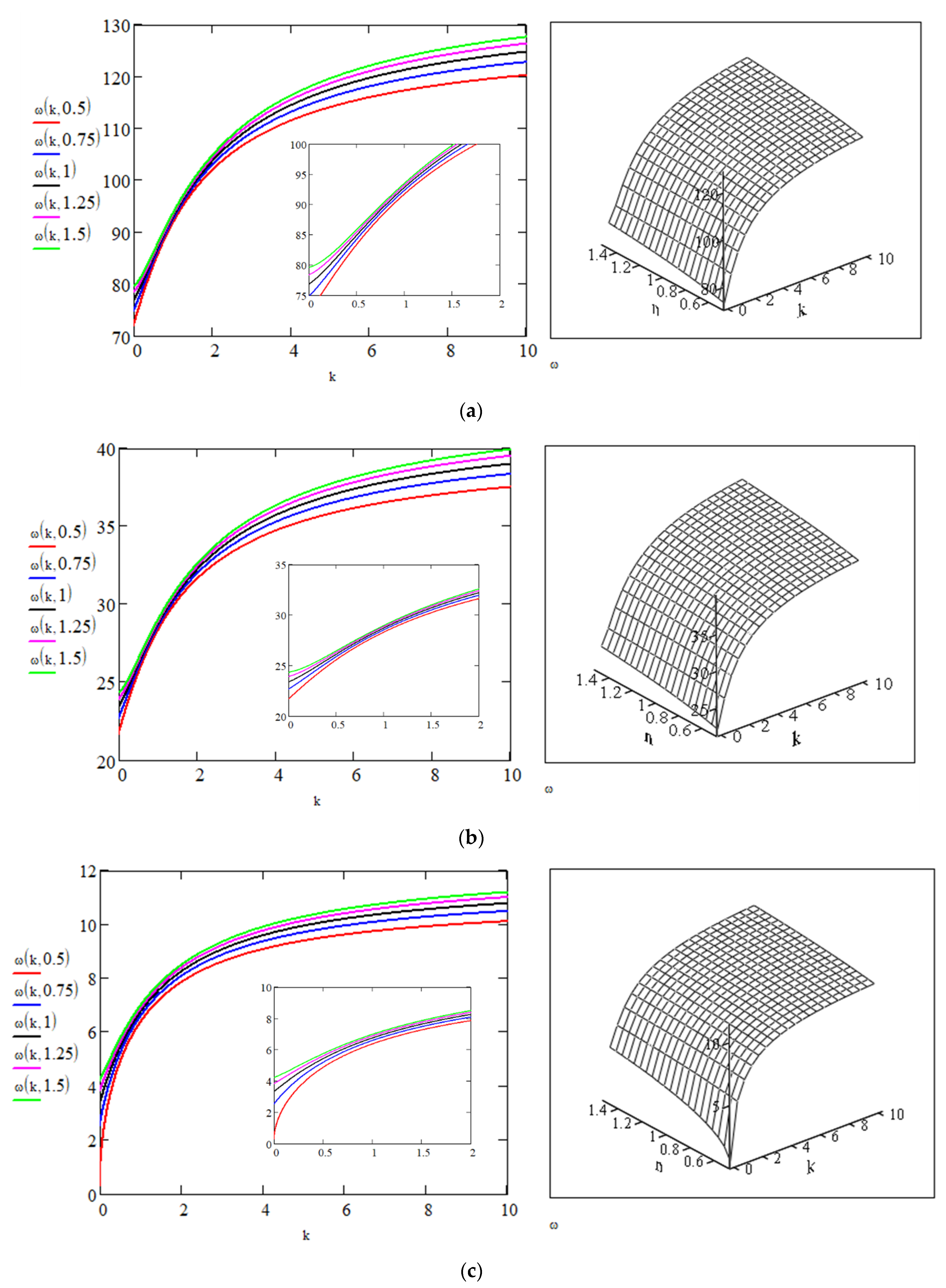
4. Natural Frequencies of Vibration
- P = 0
- P = 1.32
- P = 2.64
5. Response to Seismic Action
5.1. Generalized Structural Displacement
- P = 2.64
- ○
- ○
- ○
- ρ = 0.1
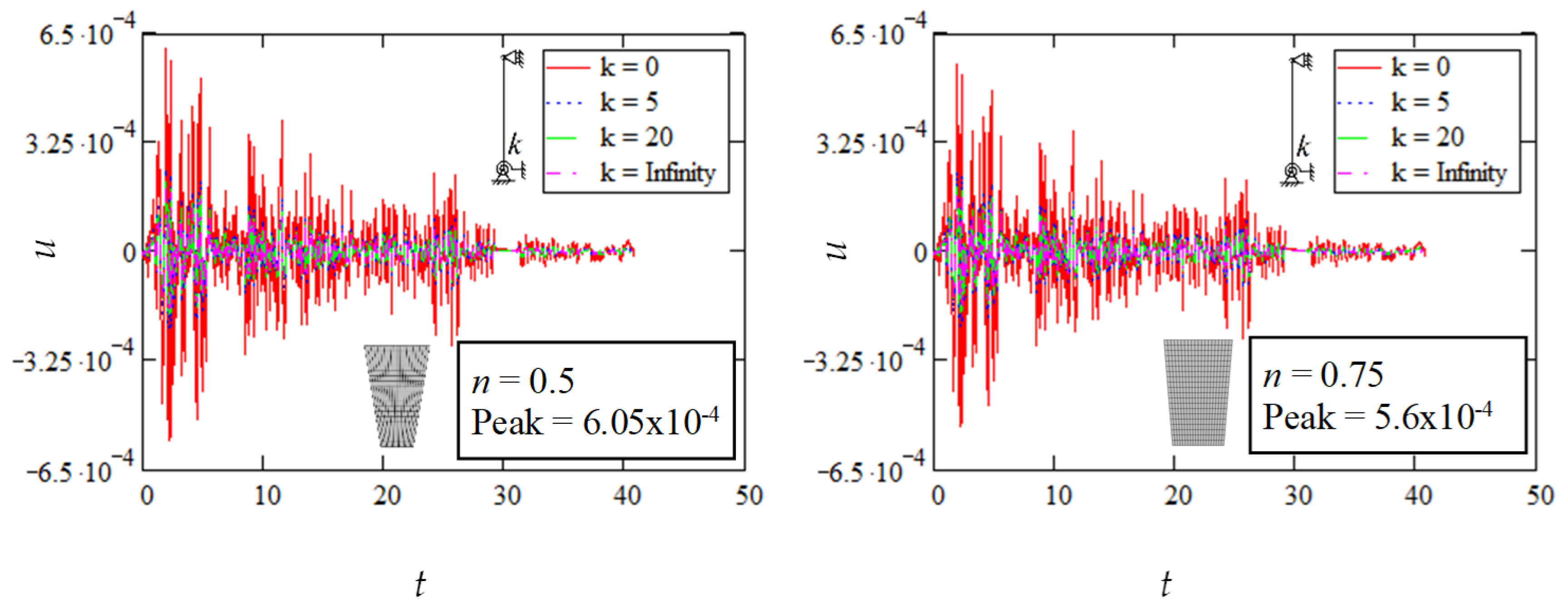


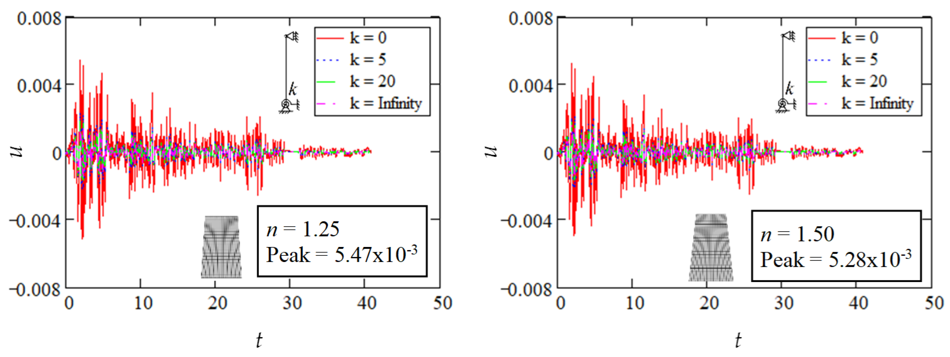
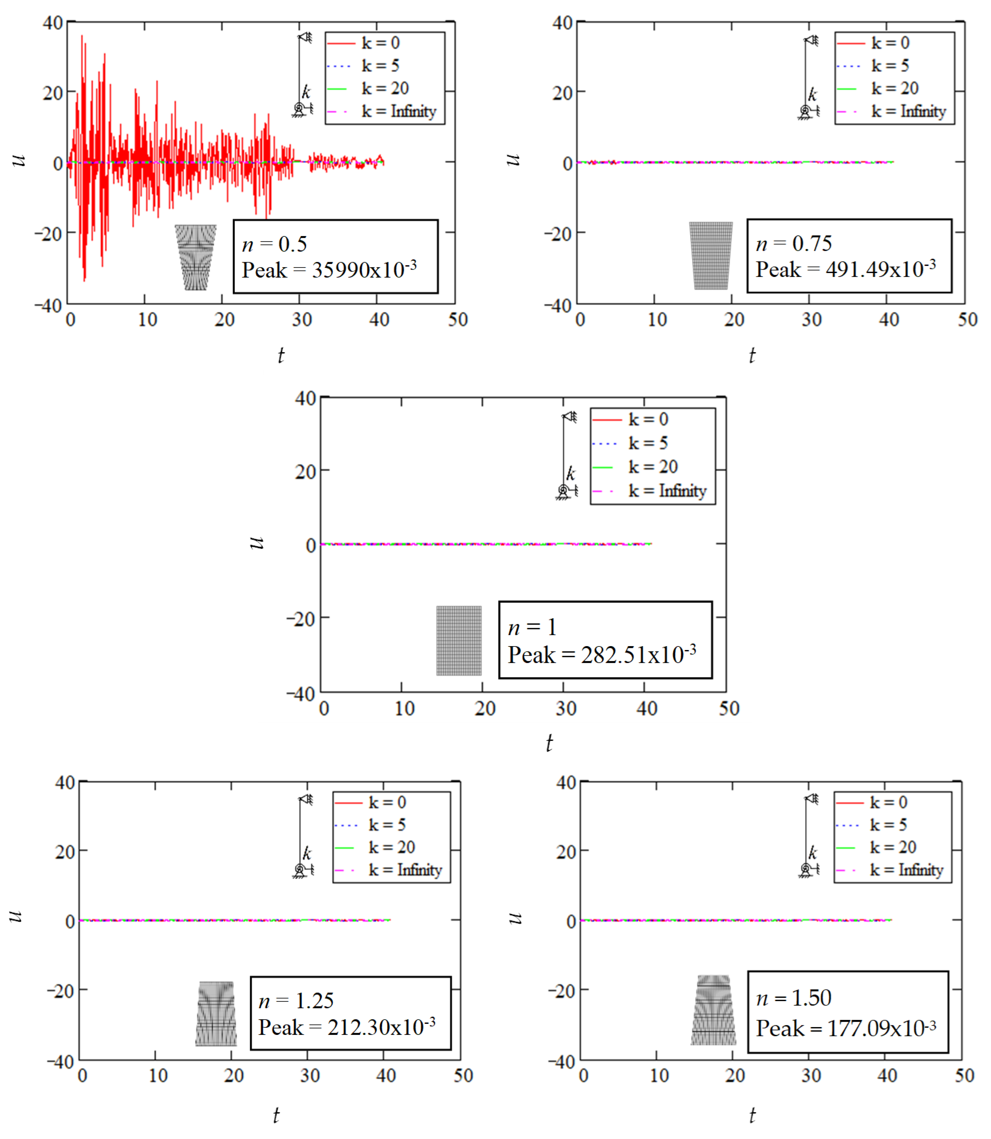
5.2. Peak Structural Movement
5.3. Structural Response Interpretation
6. Conclusions
- The natural frequency is significantly influenced by axial loading. The axial load is associated with the geometric stiffness parcel of the total generalized stiffness of the column. This means that the transversal stiffness of the columns, which is related to the lateral motion, does not depend on elasticity, but on its reluctance to change geometry, and is said to be exclusively geometric. The axial force of compression decreases stiffness and the vibration frequencies.
- Associated with the effect of axial force, it could be observed that when the density of the material increases by ten times, the frequency of the column decreases by around three times in relation to the previous value. For the same density, when the column changes shape, the frequency grows by different percentages. For P = 0, 1.91, 2.07, and 4.05 percent differences are found. For P = 1.32, these values are 3.71, 3.93, and 6.60. For P = 2.64, they are 5.79, 6.06, and 9.65.
- On the other hand, the combination of the top load equal to 2.64, considering two decimals, and the density of the material equal to 0.1 establishes the limit of axial loading to make the hinged–hinged column exist (n = 0.5). The exact value for the limit of the top load is 2.6479215086519375. At this level of force, the column frequency is zero (0.00). In this condition, the relationship between the top load and the total self-weight of the column is 0.3 (n = 0.5, ρ = 0.1). This is an important aspect that can be used in analysis by designers and researchers.
- The natural frequency depends on the shape of the column. The shape of the column is represented in formulations by the variable moment of inertia, I(y). The shape variation of the column influences both the mass distribution and the axial force, N(y), with repercussions for the geometric stiffness parcel and generalized mass of the column. At the same time, the moment of inertia is also considered inside the generalized flexural stiffness parcel—K0 of the total generalized stiffness, K. Therefore, several parameters are affected by the changing shape of the column, altering the structural response under seismic action.
- The natural frequency depends on the boundary conditions of the column. The boundary condition influences the total generalized stiffness of the structural system because it depends on the shape function assumed to represent the vibrational mode as well as the energy added by the rotational spring fixed to the base extremity. In this sense, the rotational spring alters the generalized stiffness through the shape function, and it provides an additional parcel of stiffness.
- Under seismic action, lower values of rotational base spring coefficients—around 5—reduce the displacement by around 50%, meaning that this range can exert significant influence on the structural response. For higher values, the reduction is not as significant.
- Under seismic action, when the column is close to buckling (P = 2.64, n = 0.5, ρ = 0.1), the peak displacement, velocity, and acceleration increase, signaling that the column is near to losing the stability.
Author Contributions
Funding
Data Availability Statement
Conflicts of Interest
Symbols and Abbreviations
| A | cross-sectional area, m2 |
| a, b | shape function indication |
| b | column width |
| cos | cosine function |
| d | differential |
| ( ) | function |
| d( )/d | first derivative of a function |
| d2( )/d2 | second derivative of a function |
| E | modulus of elasticity of a material, N/m2 |
| G | total self-weight, N |
| g | acceleration of gravity, m/s2 |
| I | moment of inertia of area, m4 |
| i | location along the column |
| K | total generalized stiffness, N/m |
| Kg | generalized geometric stiffness, N/m |
| K0 | generalized flexural stiffness, N/m |
| Kri | generalized stiffness of a rotational spring, N/m |
| kg | kilogram |
| M | generalized mass, kg |
| m | meter |
| m* | self-mass, kg |
| mp | concentrated mass of a force P, kg |
| N | normal force, Newton (kg.m/s2) |
| n | shape ratio |
| P | concentrated force, N |
| rad | radian |
| s | second |
| sin | sine function |
| y | geometric independent variable, m |
| γ | specific weight of the material, N/m3 |
| γp | coordinate of a force P, m |
| π | 3.14159… |
| κ | rotational spring coefficient, N/m |
| φ | shape function |
| ω | natural frequency, rad/s |
| % | percent, 1/100 |
| 0, 1 | boundary condition location |
References
- Santos, J.B.; Silva, T.J.; Salva, G.M. Influence of the stiffness of beam-column connections on the structural analysis of reinforced concrete buildings. Rev. IBRACON Estrut. Mater. 2018, 11, 834–855. [Google Scholar] [CrossRef]
- Liang, L. Seismic behavior of irregular shaped beam-column connections. Eng. Struct. 2023, 297, 116942. [Google Scholar] [CrossRef]
- Yu, M.; Yang, C.; Li, Y. Big Data in Natural Disaster Management: A Review. Geosciences 2018, 8, 165. [Google Scholar] [CrossRef]
- Xie, B.; Wu, L.; Sun, L.; Xu, Y.; Yoshikawa, A.; Mao, W. Mechanism of Multiple Anomalies Prior to Japan Earthquakes from 2021 to 2023: Lithosphere-Coversphere-Atmosphere-Ionosphere Coupling Driven by Pressure-Stimulated Rock Current. ESS Open Arch. 2025. [Google Scholar] [CrossRef]
- Annapurna, D.; Yaqubi, E.; Anuradha, P.; Radhika, K. Seismic response of RC framed irregular structures. Mater. Today Proc. 2023, 93, 530–537. [Google Scholar] [CrossRef]
- Chen, Z.; Liu, Y.; Zhong, X.; Liu, J. Rotational stiffness of inter-module connection in mid-rise modular steel buildings. Eng. Struct. 2019, 196, 109273. [Google Scholar] [CrossRef]
- Liu, X.; Meng, Q.; Xu, L.; Liu, Y.; Tian, X. Modular Steel Buildings Based on Self-Locking-Unlockable Connections Seismic Performance Analysis. Buildings 2025, 15, 678. [Google Scholar] [CrossRef]
- Zhang, J.; Yuan, W.; Zhang, T. Experimental study of earthquake resilient precast concrete beam-column-slab joints with bearing-double-stage energy dissipation connector. Soil Dyn. Earthq. Eng. 2025, 190, 109151. [Google Scholar] [CrossRef]
- EN 1998:2004; Eurocode 8—Design of Structures for Earthquake Resistance: General Rules, Seismic Actions and Rules for Buildings. European Committee for Standardization (CEN): Brussels, Belgium, 2004.
- Morano, M.; Liu, J.; Williamson, E.; Hutchinson, T.; Pantelides, C.; Saxey, B.; Richards, P. Shake table testing of a full-scale three-story seismically resilient steel-framed building with reconfigurable lateral force-resisting systems. Earthq. Spectra 2025, 41, 87552930241301424. [Google Scholar] [CrossRef]
- Gorini, D.N.; Marrazzo, P.R.; Nastri, E.; Montuori, R. Effectiveness of an innovative seismic resilient superelevation in an archetype, existing soil-structure system. Bull. Earthq. Eng. 2025, 23, 1677–1705. [Google Scholar] [CrossRef]
- Chanda, D.; Saha, R.; Haldar, S.; Choudhury, D. State-of-the-art review on responses of combined piled raft foundation subjected to seismic loads using static and dynamic approaches. Soil Dyn. Earthq. Eng. 2023, 169, 107869. [Google Scholar] [CrossRef]
- Alva, G.M.S.; Debs, A.L.H.d.C.E.; El Debs, M.K. An experimental study on cyclic behaviour of reinforced concrete connections. Can. J. Civ. Eng. 2007, 34, 565–575. [Google Scholar] [CrossRef]
- Kataoka, M.N.; Ferreira, M.A.; El Debs, A.L.H. Study on the behavior of beam-column connection in precast concrete structure. Comput. Concr. 2015, 16, 163–178. [Google Scholar] [CrossRef]
- Choi, H.-K.; Choi, Y.-C.; Choi, C.-S. Development and testing of precast concrete beam-to-column connections. Eng. Struct. 2013, 56, 1820–1835. [Google Scholar] [CrossRef]
- Xiong, X.; Wei, Z.; Zhang, D.; Liu, J.; Xie, Y.; He, L. An Experimental Study on the Seismic Performance of New Precast Prestressed Concrete Exterior Joints Based on UHPC Connection. Buildings 2025, 15, 729. [Google Scholar] [CrossRef]
- Zhang, Z.; Guo, F.; Gao, J.; Deng, E.; Kong, J.; Zhang, L. Seismic performance of an innovative prefabricated bridge pier using rapid hardening ultra-high performance concrete. Structures 2025, 74, 108558. [Google Scholar] [CrossRef]
- Ardalani, A.; Aydin, A.C. Nonlinear Seismic Performance Assessment of Energy-Based Steel Structures with Semi-Rigid Connections. Iran. J. Sci. Technol. Trans. Civ. Eng. 2025, 1–32. [Google Scholar] [CrossRef]
- Maali, M.S.; Tavlaşoğlu, M.E.; Maali, M. Experimental study on the cold-formed steel beam-to-column screw connections for seismic application. Structures 2025, 72, 108173. [Google Scholar] [CrossRef]
- Xu, J.; Gan, Z. Post-earthquake fire resistance of beam-column connection connected with high-strength steel flush end-plate. Structures 2025, 71, 108190. [Google Scholar] [CrossRef]
- Marmarchinia, S.; Azad, A.R.G.; Mirghaderi, S.R.; Karney, B.; Ali, M. A novel modular system for pipe racks using friction-slip connections. J. Constr. Steel Res. 2025, 226, 109286. [Google Scholar] [CrossRef]
- Meng, B.; Li, H.; Liew, J.-Y.R.; Li, S.; Kong, D.-Y. Enhancing the Collapse Resistance of a Composite Subassembly with Fully Welded Joints Using Sliding Inner Cores. J. Struct. Eng. 2024, 150, 04024085. [Google Scholar] [CrossRef]
- Strutt, J.W. The Theory of Sound; Re-issued 1945; Dover Publications: New York, NY, USA, 1877; Volume 1, p. 544. [Google Scholar]
- Wahrhaftig, A.d.M.; Magalhães, K.M.; Silva, M.A.; Brasil, R.M.d.F.; Banerjee, J.R. Buckling and free vibration analysis of non-prismatic columns using optimized shape functions and Rayleigh method. Eur. J. Mech. A/Solids 2022, 94, 104543. [Google Scholar] [CrossRef]
- Banerjee, J.; Jackson, D. Free vibration of a rotating tapered Rayleigh beam: A dynamic stiffness method of solution. Comput. Struct. 2013, 124, 11–20. [Google Scholar] [CrossRef]
- Ghani, S.N.; Neamah, R.A.; Abdalzahra, A.T.; Al-Ansari, L.S.; Abdulsamad, H.J. Analytical and numerical investigation of free vibration for stepped non-homogeneous cantilever beam. Open Eng. 2022, 12, 184–196. [Google Scholar] [CrossRef]
- Peng, S.; Xiong, Z.; Xu, C.-X.; Fei, J.; Chen, X. Research on shear strength of CFSST column and H-section with beam composite joint of unequal depth. J. Constr. Steel Res. 2021, 180, 106575. [Google Scholar] [CrossRef]
- Poudel, P.; Adhikari, B. Comparative Study on Seismic Behavior of Regular and Irregular Building in Sloping Ground. Himal. J. Appl. Sci. Eng. 2025, 5, 105–123. [Google Scholar] [CrossRef]
- Xu, Z.-H.; Bai, G.-L.; Zhao, J.-Q.; Liu, B. Study on seismic performance of SRC leaning beam-column exterior joints in the main workshop of CAP1400 nuclear power plant. Structures 2021, 34, 2721–2734. [Google Scholar] [CrossRef]
- Wang, B.; Dai, H.; Wu, T.; Bai, G.; Bai, Y. Study on seismic performance and influencing parameters of SRC exterior joints with the variable column in main building for thermal power plants. Earthq. Eng. Eng. Dyn. 2014, 34, 86–96. [Google Scholar]
- Zhou, Y.; Wang, X. A methodology for formulating dynamical equations in analytical mechanics based on the principle of energy conservation. J. Phys. Commun. 2022, 6, 035006. [Google Scholar] [CrossRef]
- Espí, M.V.; Bravo, J.C.; Rojas, C.O. On Galileo’s Tallest Column. Math. Probl. Eng. 2015, 2015, 649341. [Google Scholar] [CrossRef]
- Eisenberger, M.; Wahrhaftig, A.d.M. Buckling Loads of Variable Stiffness Columns Loaded by Top Load and Linearly and Parabolically Distributed Loading. Int. J. Struct. Stab. Dyn. 2024, 5, 2650001. [Google Scholar] [CrossRef]
- Ilanko, S.; Monterrubio, L.E.; Mochida, Y. The Rayleigh−Ritz Method for Structural Analysis; John Wiley & Sons, Inc.: Hoboken, NJ, USA, 2014. [Google Scholar]
- Piyapiphat, S.; Nuntasri, A.; Phungpaingam, B.; Musiket, K.; Jiammeepreecha, W.; Chucheepsakul, S. Influence of self-weight on buckling and post-buckling behavior of AFGM spring-hinged cantilever column under tip load. Mech. Based Des. Struct. Mach. 2025, 1–25. [Google Scholar] [CrossRef]
- Wang, Y.; Lv, J.; Yang, M.; Zhang, Y.; Qin, T.; Wang, L. Stability analysis of an articulated flexible pipe conveying fluid with a rotational spring. J. Fluids Struct. 2025, 133, 104277. [Google Scholar] [CrossRef]
- Wahrhaftig, A.d.M.; Eisenberger, M. Buckling load of heavy columns with variable cross section and flexible end restraints. Zamm 2024, 104, e202400626. [Google Scholar] [CrossRef]


| n | ρ | ||
|---|---|---|---|
| 0.001 | 0.01 | 0.1 | |
| 0.50 | 0.074 | 0.735 | 7.355 |
| 0.75 | 0.103 | 0.883 | 8.826 |
| 1.00 | 0.118 | 1.177 | 11.768 |
| 1.25 | 0.132 | 1.324 | 13.239 |
| 1.50 | 0.147 | 1.471 | 14.710 |
| n | Method | k = 0 | k = 1 | k = 5 | k = 20 | k = ∞ | |||||
|---|---|---|---|---|---|---|---|---|---|---|---|
| Pcr | qcr | Pcr | qcr | Pcr | qcr | Pcr | qcr | Pcr | qcr | ||
| 0.50 | Rayleigh | 7.40 | 13.74 | 10.22 | 22.81 | 13.45 | 33.81 | 14.81 | 38.32 | 15.37 | 40.11 |
| Exact | 7.26 | 12.80 | 9.14 | 17.18 | 12.13 | 25.82 | 17.07 | 47.31 | 14.72 | 34.88 | |
| 0.75 | Rayleigh | 8.64 | 16.72 | 11.46 | 27.03 | 15.33 | 41.14 | 19.33 | 56.60 | 17.80 | 49.82 |
| Exact | 8.61 | 15.75 | 10.40 | 20.04 | 13.81 | 30.03 | 21.58 | 66.12 | 17.58 | 43.93 | |
| 1.00 | Rayleigh | 9.87 | 19.74 | 12.71 | 31.29 | 17.21 | 48.66 | 23.84 | 75.82 | 20.23 | 59.88 |
| Exact | 9.87 | 18.57 | 11.60 | 22.79 | 15.28 | 33.64 | 14.81 | 38.32 | 20.19 | 52.50 | |
| 1.25 | Rayleigh | 11.10 | 22.79 | 13.96 | 35.57 | 19.09 | 56.32 | 17.07 | 47.31 | 22.66 | 70.22 |
| Exact | 11.08 | 21.30 | 12.75 | 25.46 | 16.62 | 36.93 | 19.33 | 56.60 | 22.65 | 60.75 | |
| 1.50 | Rayleigh | 12.34 | 25.87 | 15.21 | 39.88 | 20.97 | 64.09 | 21.58 | 66.12 | 25.09 | 80.77 |
| Exact | 12.25 | 23.97 | 13.88 | 28.09 | 17.87 | 40.01 | 23.84 | 75.82 | 25.00 | 68.80 | |
| k | (a) | (b) | (c) |
|---|---|---|---|
| 0 | 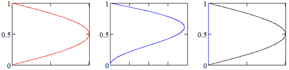 | ||
| 5 | 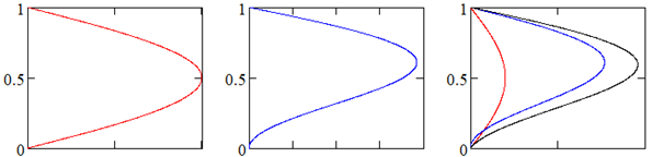 | ||
| 20 | 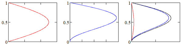 | ||
| ∞ |  | ||
| P (N) | ρ (kg/m3) | G (N) | α | w (rad/s) | w Variation (%) | |||||
|---|---|---|---|---|---|---|---|---|---|---|
| n | n | n | n | |||||||
| 0.5 | 1.5 | 0.5 | 1.5 | 0.5 | 1.5 | 0.5 | 1.5 | 0.5/0.75 | ||
| 0 | 0.001 | 0.09 | 0.15 | 0 | 0 | 133.16 | 135.75 | - | - | 1.91 |
| 0.01 | 0.88 | 1.47 | 0 | 0 | 41.65 | 42.53 | 68.72 | 68.67 | 2.07 | |
| 0.1 | 8.83 | 14.71 | 0 | 0 | 11.62 | 12.11 | 72.10 | 71.53 | 4.05 | |
| 1.32 | 0.001 | 0.09 | 0.15 | 14.67 | 0.07 | 126.85 | 131.74 | - | - | 3.71 |
| 0.01 | 0.88 | 1.47 | 1.50 | 0.01 | 39.63 | 41.25 | 68.76 | 68.69 | 3.93 | |
| 0.1 | 8.83 | 14.71 | 0.15 | 0.00 | 10.89 | 11.66 | 72.52 | 71.73 | 6.60 | |
| 2.64 | 0.001 | 0.09 | 0.15 | 29.33 | 0.07 | 120.22 | 127.61 | - | - | 5.79 |
| 0.01 | 0.88 | 1.47 | 3.00 | 0.01 | 37.51 | 39.93 | 68.80 | 68.71 | 6.06 | |
| 0.1 | 8.83 | 14.71 | 0.30 | 0.00 | 10.11 | 11.19 | 73.05 | 71.98 | 9.65 | |
| n | k | Peak Displacement | ||||||||
|---|---|---|---|---|---|---|---|---|---|---|
| P = 0 | P = 1.32 | P = 2.64 | ||||||||
| ρ = 0.001 (×10−4) | ρ = 0.01 (×10−3) | ρ = 0.1 (×10−3) | ρ = 0.001 (×10−4) | ρ = 0.01 (×10−3) | ρ = 0.1 (×10−3) | ρ = 0.001 (×10−4) | ρ = 0.01 (×10−3) | ρ = 0.1 (×10−3) | ||
| 0.5 | 0 | 3.88 | 4.12 | 107.67 | 4.72 | 5.09 | 214.70 | 6.05 | 6.65 | 35,990.00 |
| 5 | 1.99 | 2.04 | 27.23 | 2.22 | 2.28 | 31.62 | 2.50 | 2.58 | 37.70 | |
| 20 | 1.69 | 1.72 | 21.95 | 1.86 | 1.90 | 24.87 | 2.06 | 2.11 | 28.68 | |
| ∞ | 1.58 | 1.61 | 20.16 | 1.72 | 1.76 | 22.66 | 1.90 | 1.95 | 25.85 | |
| 0.75 | 0 | 3.88 | 4.10 | 100.29 | 4.58 | 4.90 | 166.58 | 5.60 | 6.09 | 491.49 |
| 5 | 1.98 | 2.03 | 26.59 | 2.17 | 2.23 | 30.19 | 2.41 | 2.48 | 34.90 | |
| 20 | 1.65 | 1.69 | 21.15 | 1.80 | 1.83 | 23.50 | 1.96 | 2.01 | 26.44 | |
| ∞ | 1.54 | 1.57 | 19.33 | 1.66 | 1.69 | 21.32 | 1.80 | 1.84 | 23.77 | |
| 1 | 0 | 3.87 | 4.10 | 95.38 | 4.48 | 4.77 | 142.61 | 5.30 | 5.72 | 282.51 |
| 5 | 1.97 | 2.01 | 26.10 | 2.14 | 2.19 | 29.15 | 2.34 | 2.40 | 33.00 | |
| 20 | 1.63 | 1.66 | 20.56 | 1.75 | 1.79 | 22.52 | 1.89 | 1.93 | 24.90 | |
| ∞ | 1.51 | 1.53 | 18.71 | 1.61 | 1.64 | 20.36 | 1.73 | 1.77 | 22.33 | |
| 1.25 | 0 | 3.87 | 4.09 | 91.88 | 4.40 | 4.68 | 128.26 | 5.09 | 5.47 | 212.30 |
| 5 | 1.96 | 2.00 | 25.72 | 2.11 | 2.16 | 28.36 | 2.28 | 2.34 | 31.60 | |
| 20 | 1.61 | 1.64 | 20.10 | 1.71 | 1.75 | 21.78 | 1.83 | 1.87 | 23.77 | |
| ∞ | 1.48 | 1.51 | 18.23 | 1.57 | 1.60 | 19.64 | 1.68 | 1.71 | 21.29 | |
| 1.5 | 0 | 3.87 | 4.08 | 89.26 | 4.34 | 4.61 | 118.70 | 4.94 | 5.28 | 177.09 |
| 5 | 1.95 | 1.99 | 25.41 | 2.08 | 2.13 | 27.74 | 2.24 | 2.29 | 30.54 | |
| 20 | 1.59 | 1.62 | 19.74 | 1.69 | 1.72 | 21.21 | 1.79 | 1.83 | 22.91 | |
| ∞ | 1.46 | 1.49 | 17.86 | 1.54 | 1.57 | 19.08 | 1.64 | 1.67 | 20.49 | |
| n | k | Peak Velocity | ||||||||
|---|---|---|---|---|---|---|---|---|---|---|
| P = 0 | P = 1.32 | P = 2.64 | ||||||||
| ρ = 0.001 (×10−4) | ρ = 0.01 (×10−3) | ρ = 0.1 (×10−3) | ρ = 0.001 (×10−4) | ρ = 0.01 (×10−3) | ρ = 0.1 (×10−3) | ρ = 0.001 (×10−4) | ρ = 0.01 (×10−3) | ρ = 0.1 (×10−3) | ||
| 0.5 | 0 | 1.68 | 1.78 | 46.69 | 2.05 | 2.21 | 93.10 | 2.62 | 2.88 | 15,610.00 |
| 5 | 1.42 | 1.45 | 19.35 | 1.58 | 1.62 | 22.47 | 1.78 | 1.83 | 26.79 | |
| 20 | 1.31 | 1.33 | 16.99 | 1.44 | 1.47 | 19.24 | 1.59 | 1.64 | 22.19 | |
| ∞ | 1.26 | 1.29 | 16.15 | 1.38 | 1.41 | 18.14 | 1.52 | 1.56 | 20.70 | |
| 0.75 | 0 | 1.76 | 1.86 | 45.45 | 2.08 | 2.22 | 75.50 | 2.54 | 2.76 | 222.77 |
| 5 | 1.43 | 1.47 | 19.23 | 1.57 | 1.61 | 21.83 | 1.74 | 1.79 | 25.25 | |
| 20 | 1.31 | 1.34 | 16.78 | 1.42 | 1.46 | 18.64 | 1.56 | 1.59 | 20.97 | |
| ∞ | 1.26 | 1.29 | 15.91 | 1.37 | 1.39 | 17.55 | 1.49 | 1.52 | 19.57 | |
| 1 | 0 | 1.81 | 1.91 | 44.58 | 2.09 | 2.23 | 66.66 | 2.48 | 2.68 | 132.05 |
| 5 | 1.44 | 1.48 | 19.13 | 1.57 | 1.60 | 21.37 | 1.71 | 1.76 | 24.19 | |
| 20 | 1.32 | 1.34 | 16.62 | 1.41 | 1.44 | 18.20 | 1.53 | 1.56 | 20.12 | |
| ∞ | 1.27 | 1.29 | 15.73 | 1.36 | 1.38 | 17.12 | 1.46 | 1.49 | 18.78 | |
| 1.25 | 0 | 1.85 | 1.96 | 43.93 | 2.10 | 2.24 | 61.33 | 2.43 | 2.62 | 101.51 |
| 5 | 1.45 | 1.48 | 19.05 | 1.56 | 1.60 | 21.01 | 1.69 | 1.73 | 23.41 | |
| 20 | 1.32 | 1.34 | 16.49 | 1.41 | 1.43 | 17.87 | 1.50 | 1.54 | 19.50 | |
| ∞ | 1.27 | 1.29 | 15.59 | 1.35 | 1.37 | 16.79 | 1.43 | 1.46 | 18.20 | |
| 1.5 | 0 | 1.88 | 1.99 | 43.43 | 2.11 | 2.24 | 57.75 | 2.40 | 2.57 | 86.17 |
| 5 | 1.46 | 1.49 | 18.99 | 1.56 | 1.59 | 20.73 | 1.67 | 1.71 | 22.82 | |
| 20 | 1.32 | 1.34 | 16.38 | 1.40 | 1.43 | 17.60 | 1.49 | 1.52 | 19.02 | |
| ∞ | 1.27 | 1.29 | 15.47 | 1.34 | 1.36 | 16.53 | 1.42 | 1.44 | 17.75 | |
| n | k | Peak Acceleration | ||||||||
|---|---|---|---|---|---|---|---|---|---|---|
| P = 0 | P = 1.32 | P = 2.64 | ||||||||
| ρ = 0.001 (×10−3) | ρ = 0.01 (×100) | ρ = 0.1 (×100) | ρ = 0.001 (×10−3) | ρ = 0.01 (×100) | ρ = 0.1 (×100) | ρ = 0.001 (×10−3) | ρ = 0.01 (×100) | ρ = 0.1 (×100) | ||
| 0.5 | 0 | 182.09 | 1.93 | 50.58 | 221.92 | 2.39 | 100.85 | 284.05 | 3.12 | 16,900.00 |
| 5 | 251.58 | 2.58 | 34.35 | 280.04 | 2.88 | 39.89 | 315.76 | 3.26 | 47.55 | |
| 20 | 252.57 | 2.58 | 32.83 | 277.60 | 2.84 | 37.20 | 308.15 | 3.16 | 42.89 | |
| ∞ | 252.44 | 2.58 | 32.30 | 276.21 | 2.82 | 36.29 | 304.92 | 3.12 | 41.41 | |
| 0.75 | 0 | 198.89 | 2.11 | 51.47 | 235.03 | 2.52 | 85.49 | 287.24 | 3.12 | 252.23 |
| 5 | 258.64 | 2.65 | 34.74 | 283.85 | 2.91 | 39.45 | 314.49 | 3.24 | 45.63 | |
| 20 | 260.05 | 2.65 | 33.24 | 282.10 | 2.88 | 36.93 | 308.23 | 3.16 | 41.55 | |
| ∞ | 260.16 | 2.65 | 32.73 | 281.04 | 2.87 | 36.10 | 305.57 | 3.12 | 40.25 | |
| 1 | 0 | 211.48 | 2.24 | 52.06 | 244.35 | 2.61 | 77.83 | 289.33 | 3.12 | 154.19 |
| 5 | 264.12 | 2.70 | 35.04 | 286.73 | 2.94 | 39.13 | 313.57 | 3.22 | 44.30 | |
| 20 | 265.77 | 2.71 | 33.55 | 285.45 | 2.91 | 36.75 | 308.28 | 3.15 | 40.62 | |
| ∞ | 266.03 | 2.71 | 33.04 | 284.63 | 2.90 | 35.96 | 306.04 | 3.12 | 39.45 | |
| 1.25 | 0 | 221.27 | 2.34 | 52.48 | 251.32 | 2.67 | 73.25 | 290.82 | 3.12 | 121.25 |
| 5 | 268.50 | 2.74 | 35.27 | 288.99 | 2.96 | 38.89 | 312.86 | 3.21 | 43.34 | |
| 20 | 270.28 | 2.75 | 33.78 | 288.05 | 2.94 | 36.61 | 308.32 | 3.15 | 39.94 | |
| ∞ | 270.63 | 2.75 | 33.29 | 287.40 | 2.93 | 35.86 | 306.39 | 3.12 | 38.87 | |
| 1.5 | 0 | 229.10 | 2.42 | 52.79 | 256.72 | 2.72 | 70.20 | 291.92 | 3.12 | 104.73 |
| 5 | 272.07 | 2.78 | 35.45 | 290.80 | 2.98 | 38.70 | 312.30 | 3.20 | 42.60 | |
| 20 | 273.94 | 2.79 | 33.97 | 290.13 | 2.96 | 36.50 | 308.35 | 3.15 | 39.43 | |
| ∞ | 274.35 | 2.79 | 33.48 | 289.61 | 2.95 | 35.78 | 306.67 | 3.12 | 38.43 | |
Disclaimer/Publisher’s Note: The statements, opinions and data contained in all publications are solely those of the individual author(s) and contributor(s) and not of MDPI and/or the editor(s). MDPI and/or the editor(s) disclaim responsibility for any injury to people or property resulting from any ideas, methods, instructions or products referred to in the content. |
© 2025 by the authors. Licensee MDPI, Basel, Switzerland. This article is an open access article distributed under the terms and conditions of the Creative Commons Attribution (CC BY) license (https://creativecommons.org/licenses/by/4.0/).
Share and Cite
de Macêdo Wahrhaftig, A.; Eisenberger, M.; Baptista Elias, C.; Malheiros Filho, L.A. Seismic Response of Variable Section Column with a Change in Its Boundary Conditions. Buildings 2025, 15, 1456. https://doi.org/10.3390/buildings15091456
de Macêdo Wahrhaftig A, Eisenberger M, Baptista Elias C, Malheiros Filho LA. Seismic Response of Variable Section Column with a Change in Its Boundary Conditions. Buildings. 2025; 15(9):1456. https://doi.org/10.3390/buildings15091456
Chicago/Turabian Stylede Macêdo Wahrhaftig, Alexandre, Moshe Eisenberger, Castro Baptista Elias, and Luiz Antônio Malheiros Filho. 2025. "Seismic Response of Variable Section Column with a Change in Its Boundary Conditions" Buildings 15, no. 9: 1456. https://doi.org/10.3390/buildings15091456
APA Stylede Macêdo Wahrhaftig, A., Eisenberger, M., Baptista Elias, C., & Malheiros Filho, L. A. (2025). Seismic Response of Variable Section Column with a Change in Its Boundary Conditions. Buildings, 15(9), 1456. https://doi.org/10.3390/buildings15091456