Article

Time-History Seismic Analysis of Masonry Buildings: A Comparison between Two Non-Linear Modelling Approaches

Department of Civil and Environmental Engineering (DICeA), University of Florence, Via di Santa Marta, 3-I-50139 Firenze, Italy
*
Author to whom correspondence should be addressed.
Buildings 2015, 5(2), 597-621; https://doi.org/10.3390/buildings5020597
Submission received: 25 February 2015 / Revised: 13 May 2015 / Accepted: 18 May 2015 / Published: 26 May 2015
(This article belongs to the Special Issue Seismic-Resistant Building Design)

Abstract

:
The paper presents a comparison between two numerical modelling approaches employed to investigate the seismic behavior of unreinforced masonry buildings with flexible diaphragms. The comparison is performed analyzing a two-story prototype tested on a shaking table at the CNR-ENEA research center of Casaccia (Italy). The first numerical model was built by using the finite element (FE) technique, while the second one was built by a simplified macro-element (ME) approach. Both models were employed to perform non-linear dynamic analyses, integrating the equations of motion by step-by-step procedures. The shaking table tests were simulated to analyze the behavior of the prototype from the initial elastic state until the development of extensive damage. The main results of the analyses are discussed and critically compared in terms of engineering parameters, such as accelerations, displacements and base shears. The effectiveness of both models within the investigated typology of buildings is then evaluated in depth.

1. Introduction

The seismic behavior of old masonry buildings can substantially differ from that of modern masonry constructions designed and built to meet aseismic design provisions. During an earthquake, both out-of-plane and in-plane seismic responses of the masonry walls are simultaneously activated. In the absence of a box-like behavior, the structural response is characterized by local failures with a widespread out-of-plane overturning of portions of walls. This has been frequently observed during past and recent earthquakes [1]. A satisfactory seismic performance of the structure, by means of the development of a global failure mode, can be achieved only if the out-of-plane collapses are prevented. In this case, the in-plane strength and deformation capacity of the walls are fully exploited, and they rule the global dynamic response of the building. In this respect, it is widely recognized that adequate masonry quality, proper connections between masonry walls and between walls and floors are effective measures able to prevent the local failures [2,3,4]. Among them, a significant role in coupling the response of the different masonry walls is played by the in-plane stiffness of the diaphragms (typically timber floors).
These few remarks point out the attention that must be paid by researchers when they analyze the seismic behavior of existing masonry buildings through global numerical models. Although in some cases simplified partial models could be used, a global model can better analyze the seismic response of the structure provided that a proper modelling of walls and floors is performed.
Dealing with the analysis methods, the largest part of them can be divided into three main categories: (i) the modal analysis, usually based on linear models, combined with the concept of structural behavior factor q to account for the energy dissipation effects; (ii) the non-linear static analysis (pushover); and (iii) the non-linear time-history analysis [5,6,7]. The first method is commonly adopted in the professional context, to verify the compliance of the performance level with the one required by the technical standards. Anyway, it is not fully appropriate for a reliable prediction of damages occurring in the building under earthquake loading. The pushover analysis is a procedure used to obtain the capacity diagram, which represents a basic datum to predict the strength and the ductility of the structure. In recent times, the method has become quite widespread also in engineering practice. Nevertheless, since this approach is based on a non-linear static procedure where the external loads are monotonically increased up to failure, it neglects many significant aspects of the structural response, like the damage produced by reversal loads. In addition, in the case of in-plane flexible diaphragms, even when proper connections between walls and floors prevent the local out-of-plane mechanisms, the masonry façades can exhibit an independent behavior, thus highlighting critical issues in a reliable employment of the pushover approach [3,8]. The time-history non-linear analysis method foresees a direct step-by-step integration of the equations of motion in the time domain. Provided that both a reliable non-linear numerical model of the building and a proper modelling of the seismic input are assured, this method can cover the drawbacks of the first two procedures, being able to follow the full seismic loading process (from the initial state, through the weakly non-linear behavior under service loading, up to the strongly non-linear behavior leading to collapse).
In this respect, several authors [2,3,9] have discussed the need to perform non-linear time-history analyses to reproduce the energy dissipation processes that develop in masonry buildings during the seismic event. At the same time, they showed that the use of three-dimensional finite element (FE) models requires a great amount of computational resources, which may be justified only in the case of historical and/or monumental buildings [9,10,11]. Analyzing traditional buildings, the need emerges for simplified, but effective (and reliable) models for the assessment of the global structural response through non-linear time-history analysis methods. Nevertheless, given the great variety of geometries, construction typologies and materials used to date, an analysis tool suitable for the analysis of all of the typologies of masonry buildings is not available. In the last few decades, for instance, an increasing development of simplified masonry modelling based on the macro-element [12] and the equivalent frame approaches [13,14,15] has taken place. These methods require a moderate computational effort, if compared with the traditional finite element technique. However, despite the apparent simplicity, each analysis tool requires high expertise to effectively understand its range of employability.
The above-mentioned remarks explain the difficulties that arise during the seismic assessment of existing masonry buildings. Within this framework, the paper reports the comparison between two numerical approaches employed to investigate the seismic response of traditional unreinforced masonry (URM) buildings. As a reference case study, an unreinforced masonry building (tested by a shaking table at the CNR-ENEA research center of Casaccia near Roma, in Italy) was analyzed by developing two different three-dimensional (3D) models. The first model refers to the FE technique and was built with the commercial code ANSYS [16]. The second one was based on the macro-element approach through the implementation of a non-linear algorithm in the MATLAB tool [17]. A simple identification procedure was used to define the most important masonry constitutive parameters required by the two models. To this aim, the available results by the laboratory tests performed at the CNR-ENEA center on units, mortar and diagonal compression tests on masonry wallettes were used. After identification, the two models were employed to perform linear and non-linear analyses in the time domain, by using as input the acceleration histories applied at the base of the prototype during the shaking table tests. The results obtained with the two models are compared and discussed analyzing floor accelerations, floor displacements, base shears, stiffness decay and failure modes. The comparison between experimental and numerical results was presented in a previous paper [18], to which the interested reader is referred.

2. The Masonry Building Prototype

The building assumed as a case study is one of the two masonry prototypes built at the CNR-ENEA research center of Casaccia, near Roma (Italy). The two buildings, tested through an extensive experimental investigation on a shaking table, were built within a research project partially funded by the Italian Ministry for Research [19]. The project aimed at assessing the seismic performance of scaled structures made with the typical materials and the constructive techniques employed in old masonry buildings in Central Italy. The first prototype (RM) was strengthened with the CAM system (active confinement of masonry), then it was tested to verify the effectiveness of the reinforcement; the second one (URM) was tested until collapse without any strengthening [20,21]. The prototype herein analyzed is the unreinforced one.

2.1. Geometry of the Prototype

The prototype is a 1:1.5-scaled two-story building (Figure 1), aimed at reproducing the typical ancient masonry buildings of Central Italy. The plan layout is made of a single cell with outer dimensions of 3.5 m × 3 m (Figure 2), while the inter-story heights measure approximately 2.2 m. A further masonry ring 0.15 m high is present at the top of the building, so the total height of the prototype is 4.55 m. The masonry walls have a constant thickness of 0.25 m and are composed of two vertical faces without any transversal connection (Figure 3). The horizontal structures are made with flexible timber floors. Each floor was built using five wooden joists (with a section of 0.10 m × 0.18 m) and wooden boards with a thickness of about 20 mm nailed to the wooden beams.
Figure 1. View of the unreinforced masonry (URM) prototype.
Buildings 05 00597 g001
Figure 2. Plan dimensions (cm) of the prototype: (a) first floor and (b) second floor.
Buildings 05 00597 g002
Figure 3. Masonry texture and section of the walls of the prototype.
Buildings 05 00597 g003
The total weight of the masonry is about 169.71 kN. The prototype was constructed on a reinforced concrete (RC) beam having a height of 0.4 m and a weight of 28.25 kN. The weight of the wooden floors is about 4.08 kN, and in addition, to meet the similitude scaling laws, a distributed mass of 2.5 t was placed on each floor. Hence, the total weight of the prototype over the shaking table, including the RC beam, is about 251.14 kN.
The masonry walls were constructed with calcareous tuff stones and lime-cement mortar with weight ratios of the components of 10.5 (sand), 11 (lime) to 1 (cement). The masonry units have an irregular shape and have dimensions varying from medium to large (Figure 3). The walls have a double vertical layer section with opus incertum texture. The average dimensions of the mortar joints were built intentionally very large both in the face and in the section. No connection between the two layers was provided. Furthermore, again in order to reproduce a poor constructive system, the walls were not connected together at the corners, and no concrete beams were realized to connect the wooden floors with the walls. A timber lintel was provided over each opening.

2.2. Mechanical Properties of the Masonry

Both destructive and non-destructive tests were preliminarily carried out on the units in order to characterize the masonry. Several samples of calcareous tuff stones were tested to evaluate the average compressive strength (fbc) and the specific mass (γm). The obtained values were fbc = 8.5 N/mm2 and γm = 1700 kg/m3. Laboratory tests on mortar provided the average compressive strength (fmc) and the flexural strength (fmf) equal to 0.72 and 0.14 N/mm2, respectively. Further tests on the mortar joints were performed by the PNT-G penetrometric method [22] to assess the mortar quality; results provided an average value fmc = 0.54 N/mm2. To evaluate the compressive strength of the masonry assemblages (fwc) starting from the properties of units and mortar, several relationships have been proposed [23]. Generally, these formulas are reliable only for masonries with regular texture; thus in the present case, it is only possible to obtain a feasible range of variability of this parameter. Considering fbc = 8.5 N/mm2 and fmc = 0.72 N/mm2, it is reasonable to assume that fwc ranges from 2.0 to 3.5 N/mm2 [24].
In addition to the tests on units and mortar, the masonry was characterized through three diagonal compression tests carried out on masonry wallettes. These were built with the same technique, materials and workers employed to realize the building prototypes. The wallettes were square panels with a side equal to 0.9 m and a thickness of 0.25 m. Firstly, a compressive load was applied on two opposite sides of each panel, then the diagonal load Pd was applied under displacement control up to collapse. The three panels, named MT1, MT2 and MT3, were tested imposing different values of the pre-stress (0.1, 0.15 and 0.20 N/mm2, respectively). Results in terms of maximum diagonal load were 37.1, 27.8 and 51.5 kN for the three tests. Considering the classical interpretation of the diagonal compression test, the tensile strength of the masonry ranges from 0.06 to 0.07 N/mm2 (the interested reader can refer to [18,24] for the formulation employed to estimate the compressive and the tensile strength of the masonry).

2.3. Experimental Failure Mode

To test the URM prototype, a 4 m × 4 m shaking table with six degrees-of-freedom (DOFs) was employed. The motion was impressed by eight hydraulic MTS dynamic jacks. The tests were carried out through the application of a normalized natural seismic input scaled at increasing intensity. The reference input was the accelerogram of Colfiorito (Perugia, Italy), recorded during the Umbria-Marche earthquake of 26 September 1997 (Richter magnitude of 6.1, epicenter in Annifo-Colfiorito, with peak ground acceleration (PGA) = 2.117 m/s2 for the north-south (NS) component, 2.473 m/s2 for east-west (EW) and 1.805 m/s2 for up-down (UD); Figure 4). To be consistent with the reduced scale of the structure, the original records were scaled along the time axis by a factor equal to the square root of the geometric scale of the model: 3 / 2 = 1.225 [20]. The NS, the EW and the UD components were applied simultaneously (NS and EW in y and x directions, respectively; see Figure 2).
Figure 4. Colfiorito north-south (NS), east-west (EW) and up-down (UD) ground acceleration time histories.
Buildings 05 00597 g004
During the tests, due to a system pump malfunction, the accelerations recorded on the shaking table were slightly altered with respect to the target input (nominal PGA in the following) [21,25,26]. The numerical analyses discussed next, although performed assuming as input the effective accelerations recorded on the shaking table, are referenced by employing their nominal PGA input value. Keeping in mind this distinction, the tests were carried out by applying the ground accelerations with increasing PGA (nominal increment of 0.05 g), starting from a low intensity (nominal PGA of 0.05 g) up to collapse (nominal PGA of 0.50 g).
During the first two shaking table tests (nominal PGA of 0.05 and 0.10 g), no damage was observed; the development of a vertical crack, approximately 1 cm thick, was first observed in the upper part of the corner between the walls CD and AD during the test with nominal PGA = 0.15 g (Figure 5a). The crack developed starting from the upper level, due to the thrust of the wooden floor. Out-of-plane flexural deformations were observed on the second level of the wall AB.
Figure 5. Vertical crack in the corner between the façades AD and CD after the tests with nominal PGA of (a) 0.15 g and (b) 0.25 g.
Buildings 05 00597 g005
During the test corresponding to a nominal PGA of 0.20 g, the effects observed in the previous test were accentuated, adding a strong flexural deformation on the wall BC (Figure 6a).
In the dynamic test with a nominal PGA of 0.25 g the crack on the corner between the walls CD and AD increased and widened from the roof top down to the first level (Figure 5b). At the end of the test, the crack thickness was about 3–4 cm, and fragments of mortar and stone dropped down due to the walls pounding after detachment of the corner. Diagonal cracks developed on the wall AB from the top of the façade reaching the corners in the openings. The vertical load carrying capacity of the structure was not yet compromised.
In the subsequent dynamic test (nominal PGA of 0.30 g), the corner between the walls CD and AD was completely detached, and a major crack was observed between the walls CD and BC. In addition, a cracking pattern was visible on the wall BC that extended above the timber lintel over the second level opening.
The test with nominal PGA of 0.35 g showed the worsening of previous cracks: the wall AD was completely detached from the orthogonal one (Figure 7a), while the upper part of the façade AB was subjected to considerable out-of-plane displacements with subsequent expulsion of some stone units. At the end of this test, not only the spandrels, but also the masonry piers appeared significantly damaged, specifically on the second level.
Figure 6. Diagonal cracks in the façade AB ((a) PGA = 0.20 g) and vertical crack in the façade AB ((b) PGA = 0.25 g).
Buildings 05 00597 g006
Figure 7. Façade CD cracks after failures of the corners of the second level ((a) PGA = 0.35 g) and failure of the lintels ((b) PGA = 0.45 g).
Buildings 05 00597 g007
The test with nominal PGA of 0.40 g was characterized by a strong global damage of the structure, with the collapse of the two corners of the wall CD and the collapse of the masonry pier supporting the lintel over the second floor opening. In addition, the already cracked corner of the wall AB partially collapsed. At this stage, the timber floors were completely detached from the load-bearing walls, compromising the box-behavior.
Two additional tests were then performed to assess the building residual capacity. The first test (nominal PGA = 0.45 g) showed the simultaneous collapse of all of the piers of the wall AB at the second level, as well as the lintel over the opening of the wall CD. The second test (nominal PGA = 0.5 g) was performed to achieve total structural collapse.
Figure 5, Figure 6 and Figure 7 show the prototype during the dynamic tests.

3. Numerical Models of the Prototype

To simulate the dynamic behavior of the unreinforced masonry prototype, two different numerical approaches were employed. The first 3D numerical model was built by the finite element (FE) technique, employing the commercial code ANSYS [16]. The non-linear behavior of the masonry was reproduced through a smeared crack approach, and the mechanical parameters were evaluated on the basis of the experimental results by means of an identification procedure. The second model was built by the macro-element (ME) approach implementing non-linear laws of the masonry in the MATLAB tool. The parameters required by the macro-element model were assessed comparing its modal behavior with the one obtained by the FE model.

3.1. The Finite Element Model

The macro-modelling technique was employed, as it is fit for large size models. The units and the mortar joints were hence assumed to be smeared, and a homogenous isotropic material represented the masonry assemblage. Eight-node isoparametric solid elements (Solid65) were used to model both the masonry walls and the RC basement. The wooden joists were modelled by using one-dimensional two-node isoparametric elements (Beam44) while isoparametric two-dimensional elements with four nodes (Shell63) were adopted for the wood planking. Further zero-dimensional one-node elements (Mass21) were inserted on each floor to consider the additional masses. Specific weights of masonry and wood were assumed based on the experimental data (γw = 14.2 kN/m3 and γl = 5.9 kN/m3, respectively). The final numerical model (Figure 8) consisted of 11,081 nodes, 6824 3D Solid45 elements, 94 2D Shell63 elements, 291 1D Beam44 elements and 25 0D Mass21 elements, corresponding to 30,933 degrees of freedom (DOFs).
The constitutive behavior of the masonry was reproduced assuming an elastoplastic law with tension cut-off. To this aim, the Drucker–Prager (DP) plasticity model was combined with the Willam–Warnke (WW) failure criterion. The DP yield surface is a smooth version of the Mohr–Coulomb yield surface, defined by two parameters: the cohesion c and the internal friction angle φ. They are introduced in such a way that the circular cone of DP corresponds to the outer vertex of the hexagonal Mohr–Coulomb yield surface (Figure 9) [27]. The combination of the plasticity model with the failure criterion allows for an elastic-brittle behavior in case of biaxial tensile stresses or biaxial tensile-compressive stresses with a low compression level. On the contrary, the material behaves as elastoplastic in the case of biaxial compressive stresses or biaxial tensile-compressive stresses with a high compression level. Overall, the material behaves as an isotropic medium with plastic deformation, cracking and crushing capabilities [27,28].
Figure 8. Finite element (FE) model of the URM prototype: (a) external and (b) internal views.
Buildings 05 00597 g008
Figure 9. Drucker–Prager yield surface in the Haigh–Westergaard stress space.
Buildings 05 00597 g009
The constitutive parameters required by the DP and the WW models were identified by the diagonal compression test MT1. An FE model of the square panel was built by 3D Solid65 elements, and was employed to reproduce the experimental force-vertical displacement curve. The parameters were identified through direct comparison between the experimental curve and the numerical one. The non-linear parameters are reported in Table 1, whereas the linear parameters are as follows: longitudinal modulus of elasticity Ew = 700 N/mm2, tangential modulus of elasticity Gw = 280 N/mm2 and Poisson ratio ν = 0.25. The identified tensile strength of the masonry (fwt) is within the range estimated by using the classical interpretation of MT1 and MT3 tests [24,29].
Table 1. Finite element (FE) model parameters (fwc = masonry compressive strength; fwt = masonry tensile strength; βc = shear transfer coefficient for closed cracks; βt = shear transfer coefficient for open cracks; c = cohesion; δ = dilatancy angle; φ = internal friction angle).
Drucker–Prager Plasticity CriterionWillam–Warnke Failure Surface
c (N/mm2)0.07fwc (N/mm2)2.50
δ (°)20fwt (N/mm2)0.065
φ (°)40βc (-)0.75
--βt (-)0.15
The FE model of the whole building was preliminarily employed to evaluate the modal shapes by means of a modal analysis. Results show that the first modal shape is a pure translation in the x direction with a frequency of 9.03 Hz; the second modal shape is a pure translation in the y direction with a frequency of 9.37 Hz; and the third one is a torsional mode with a frequency of 15.32 Hz (Table 2).
Table 2. Modal shapes and frequencies.
Modal ShapeDirectionFE ModelME Model
Frequency (Hz)Frequency (Hz)
1x9.039.07
2y9.379.37
3Torsional15.3212.13

3.2. The Macro-Element Model

The second model was built by the macro-element (ME) approach. This model, originally proposed by Galano and Selleri ([17]), performs a 3D step-by-step dynamic analysis of regular masonry buildings subjected to a base ground acceleration (components in two orthogonal directions can be applied simultaneously). Each masonry wall is represented by piers (with vertical axis and height equal to the inter-story) and spandrels (with horizontal axis); however, only the piers are considered as deformable and resisting elements, whereas the spandrels have infinite stiffness and strength. The diaphragms are assumed rigid in their plane; hence, the model has three DOFs for each floor, and the masses must be concentrated or distributed over these floors. The bending failure mode and the shear failure mode with diagonal cracking are considered for each pier subjected to shear load in its plane, and a simplified trilinear diagram of shear V vs. drift δ is used for each failure mode, as illustrated in Figure 10. This figure also shows a sample of the hysteretic response under reversal loads with progressive damage depending on the position of the focal point F. A similar behavior is assumed for the piers subjected to out-of-plane flexure. A detailed explanation of the main features of the numerical procedure is reported in [17]. As usual, in the shear-type models, the piers behave as masonry panels constrained by double bending conditions; this hypothesis is unrealistic, especially for existing buildings with timber floors. Hence, rotational elastic springs between piers and floors were introduced in the model to reduce the shear stiffness of the panels. The four façades of the macro-element model of the prototype are depicted in Figure 11 with the indication of the piers (13 elements) and the spandrels (12 elements, denoted by “×”).
Figure 10. (a,b) Hysteretic model for piers and (c) failure modes: (1) bending failure; (2) diagonal cracking failure; and (3) sliding shear failure.
Buildings 05 00597 g010
Figure 11. Macro-element (ME) model: definition and numbering of the piers.
Buildings 05 00597 g011
Values of the parameters used in the ME model are: Ew, Gw, γw and γl as in the finite element model, fwc = 2.5 N/mm2, fwt = 0.065 N/mm2, ultimate drifts δu in the range from 7.5 mm up to 12.5 mm (from 0.34% up to 0.57% of the inter-story height), depending on the pier slenderness and the failure mode, and Vu and VF equal to 0.25 Vmax (Figure 10). In addition, the model requires defining the distribution of the masses and the values of the elastic stiffness of the rotational springs between piers and floors.
These parameters were selected by comparison with the modal results obtained by the FE model. A fraction of 4/11 of the pier masses of the first level was attributed to the first floor (the remaining part of 7/11 rests on the foundation), and a fraction of 7/11 of the pier masses of the second level was attributed to the first floor (the remaining part of 4/11 was placed on the top floor). The additional masses were applied on the corresponding floor. Rotational springs were introduced only for piers denoted by 3, 4, 10 and 11, which are the most relevant to define the dynamic response of the model. Table 3 collects the total masses and the coordinates of the center of mass in each floor, xG and yG.
The agreement between the two models both for modal shapes and frequencies was acceptable (Table 2). Further confirmations of the accord between the two models in the elastic range were obtained performing step-by-step dynamic analyses under base input seismic accelerations. Acceptable differences (less than 5%) were obtained, for instance, for the displacements of the second floor.
Table 3. Macro-element (ME) model parameters.
FloorMass (t)xG (m)yG (m)
111.3441.761.56
26.9461.751.63
Total18.290--

4. Linear and Non-Linear Time-History Results

4.1. Seismic Input and Numerical Analyses

The dynamic responses of the two models were first compared in the linear field by considering the input corresponding to the six shaking table tests with increasing nominal PGA of 0.05, 0.10, 0.15, 0.20, 0.25 and 0.30 g. Taking into account the previously mentioned differences between the target original input signals (nominal PGA) and the effective output signals recorded on the shaking table, non-proportional responses were expected (and justified) increasing the nominal input PGA.
The input of the above six tests, and that of the two additional tests with nominal PGA of 0.35 and 0.40 g, were subsequently considered in the hypothesis of non-linear behavior. The base accelerations were selected in order to reproduce the behavior of the building starting from the elastic response up to the range going from moderate to severe damage (the FE model collapsed during the test with nominal PGA of 0.40 g; collapse is here referred to as non-convergence of the numerical solution).
Only the first 10 s in the reduced time scale of the base acceleration records were used as input, because the shock has its maximum ground acceleration intensity within the first 5 s, and it is not significant after 10 s. The responses of the FE model were computed by the Newmark integration method with a time step of 0.004 s, whereas the α-Hilbert procedure [17] with a time step of 0.001 s was employed to calculate the responses of the macro-element model. These choices provided sufficient accuracy of the solutions and acceptable computational effort. Damping was considered by the classical Rayleigh formulation, and a 4% damping ratio on the first two modal shapes was selected as suggested in the literature [30].

4.2. Response of the Linear Elastic Models

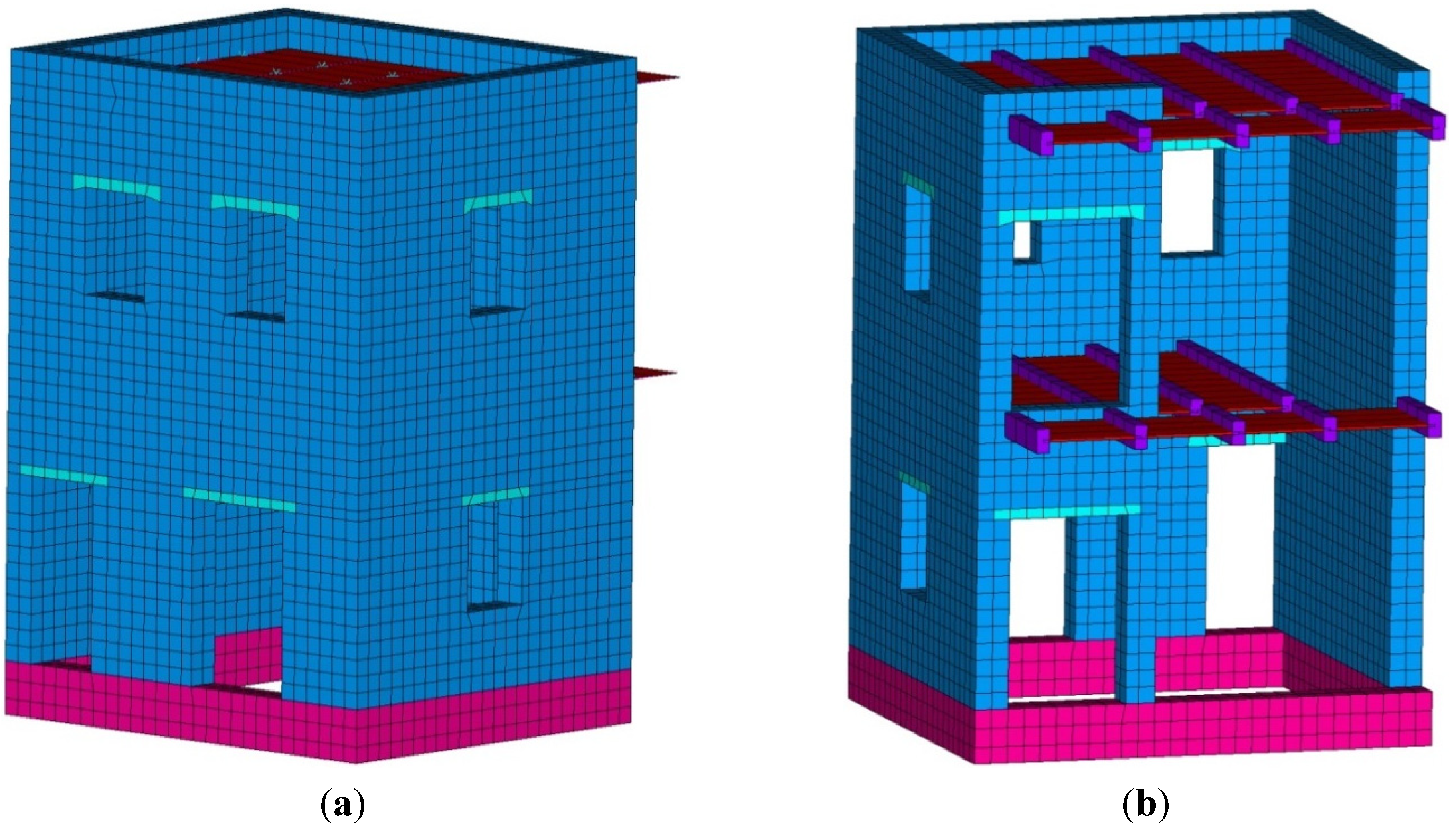
Displacements and absolute accelerations at the floor levels are two of the most significant global kinematic parameters that synthesize the dynamic response of a building. In the macro-element model, each floor moves in its plane as a rigid diaphragm, while in the FE model, the timber floors are modelled as flexible diaphragms. Consequently, to perform a significant comparison, average response parameters were considered.
Denoting with s i ( t ) 
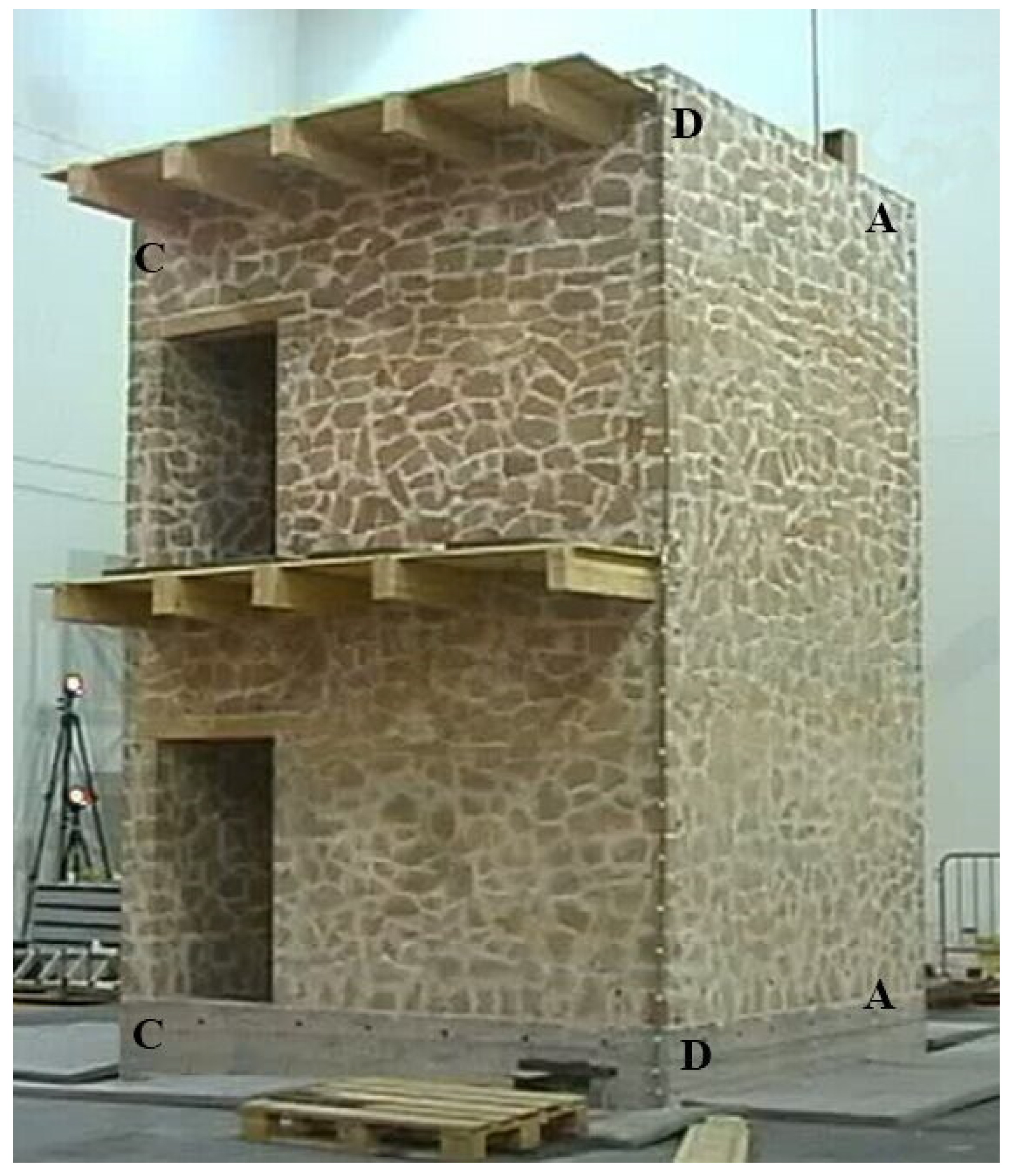
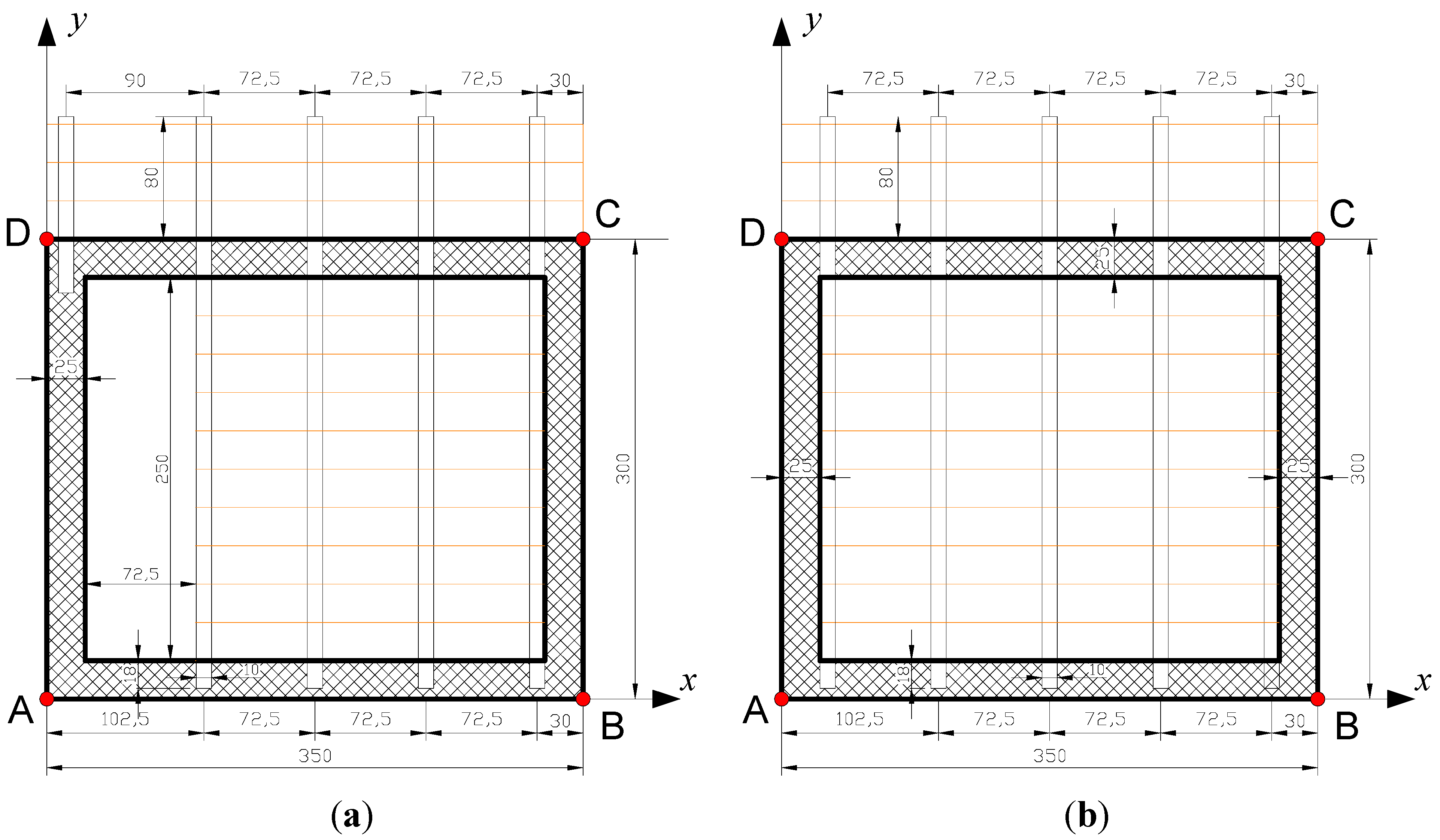
the responses (accelerations or displacements) of the four corners A, B, C and D (Figure 2), the average response s ¯ ( t ) was directly calculated as follows:
s ¯ ( t ) = 1 4 i = A , D s i ( t )
To offer a synthetic representation of each average response over the whole time-history, a representative value, called “efficacy”, was calculated by the following expression:
s e f f = 1 T m a x 0 T m a x [ s ¯ ( t ) ] 2 d t
where Tmax denotes the time length of the signal.
The agreement between the numerical responses of the two models was estimated by comparing the percentage errors defined as follows:
E s = 100 · ( s e f f M E s e f f F E ) s e f f F E
According to the definition of Equation (3), it is implicitly assumed that the response of the FE model is considered as the reference in the comparisons.
The average errors obtained simulating the first six tests for displacements (Ed), absolute accelerations (Ea) and dominant frequencies of response displacement signals (Efrd), together with the variation coefficients, are summarized in Table 4.
Considering the significant differences between the ME and the FE models, it is possible to observe a satisfactory agreement in the amplitude of the displacements (max. error equal to 20.6%) and a perfect agreement in the frequencies. In addition, it is observed that the ME model always provides slightly higher displacements values, with more pronounced differences for the first floor in the y direction.
Table 4. Average (Mean) and coefficient of variation (Cv) of percentage errors (linear analyses).
FloorDisplacements EdAccelerations EaFrequencies Efrd
Mean (%)CvMean (%)CvMean (%)Cv
F1x11.10.1119.90.7400
F1y20.60.0256.60.0400
F2x3.00.61−6.41.2400
F2y4.10.0514.10.1000
More pronounced differences were instead obtained in terms of accelerations (max. error equal to 56.6% for the first floor in the y direction). Again, the errors are always positive with the exception of the second floor in the 
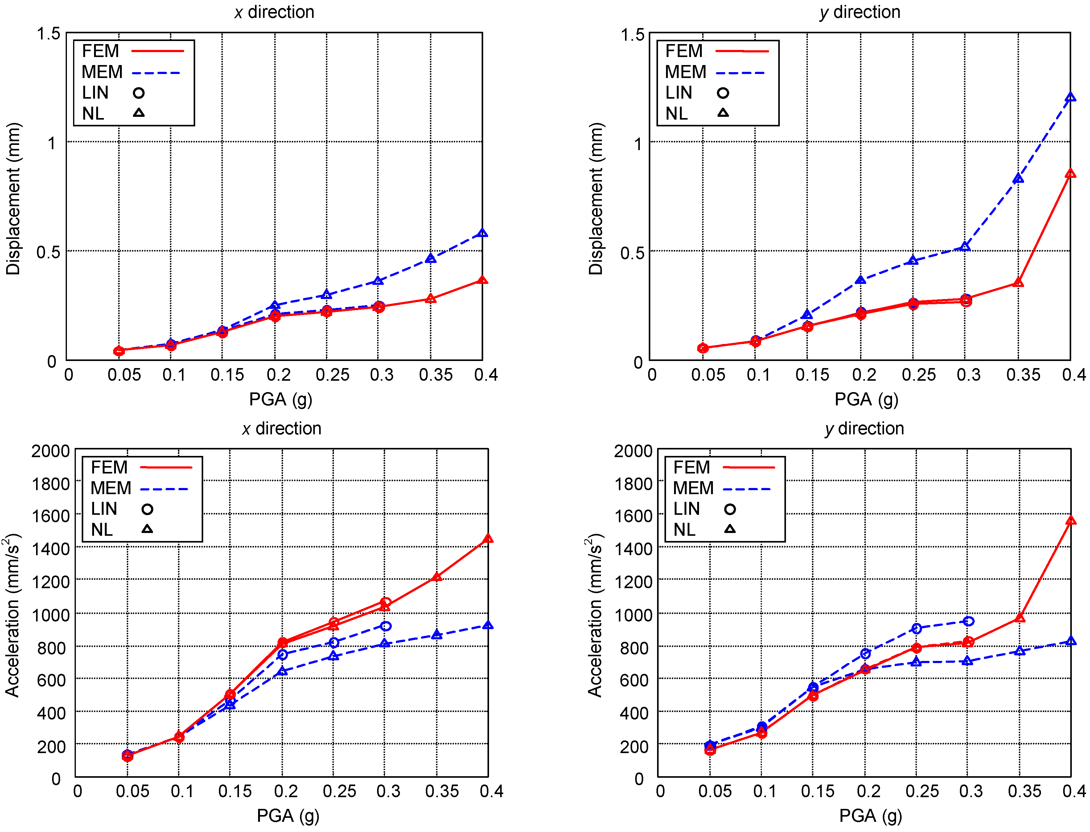
x direction. In this case, the errors obtained in the simulations with input PGA of 0.05 and 0.10 g are slightly positive; the others are negative, hence resulting in a very high variation coefficient (1.24). As an example, the efficacy displacements and accelerations, evaluated according to the definition introduced by Equation (2), of the second floor vs. the target input PGA are plotted in Figure 12 (the figure shows also the same values obtained with the non-linear models, as discussed next).
The other two main response parameters to be considered for engineering purposes are the shear forces (base shear and shear at the base of the second level, in each direction) and the stiffness of the building. For linear models, it is appropriate to evaluate the maximum absolute value of the shear as follows:
V m a x = max | V ( t ) |
and, consequently, the percentage error:
E V = 100 · ( V m a x M E V m a x F E ) V m a x F E
Figure 12. Efficacy values of displacements and absolute accelerations vs. PGA (second floor).
Buildings 05 00597 g012
The calculation of the stiffness of the building by means of the results of a time-history analysis is rather complicated, even in the case of linear behavior, because in multi-degrees-of-freedom (MDOF) models, the dynamic response is composed of a set of many displacements and forces, each of them defined in the time domain. In the present case, the stiffness was computed as secant stiffness at the origin.
Starting from the cyclic response shear V vs. inter-story drift d of a level in a direction, the envelope diagram was considered, and then, in this diagram, the secant stiffness Ks = V/d corresponding to the absolute maximum value of d was taken. This parameter is then representative of the stiffness of that level in the instant of maximum amplification of the response.
Errors were calculated according to the following equation:
E K = 100 · ( K s M E K s F E ) K s F E
Table 5 summarizes the averages of the errors EV and EK. They are always negative, i.e., the ME model provides lower values than the FE model. In particular, the stiffness of the second level in the y direction is noticeably higher for the FE model, while in the x direction, a very high coefficient of variation (0.92) is obtained. In turn, these differences explain the errors obtained in maximum shear forces (up to 30.5% for the second level in the y direction). The differences in the mass distribution between the two models can partially explain this disagreement.
Figure 13 plots the base shears and the stiffness of the building vs. the target input PGA (the figure shows also the same values obtained with the non-linear models, as discussed next).
Figure 13. Maximum base shears and secant stiffness vs. PGA.
Buildings 05 00597 g013
On the whole, the macro-element model provides dynamic responses affected by acceptable errors with respect to FEM. This suggests that in all structural problems in which the intensity of the dynamic loading is low and an almost elastic structural response is expected, the use of a simplified model, such as the one employed here, is the most acceptable choice. This is true both for the ease of use (the construction of the numerical model) and for the small computational times (each time-history analysis performed with the FE model required about 7 h against the about 5 min required by the ME model). As an example, the ME model can be an effective tool for analyzing the response of secondary elements supported by the floors of a masonry building under low to moderate earthquakes (museums, history archives, etc.). On the other hand, given the errors obtained for the base shears, the use of the FE model is more appropriate for structural analyses aimed at investigating the seismic safety.
Table 5. Average (Mean) and coefficient of variation (Cv) of percentage errors (linear analyses).
LevelShear Forces EVStiffness EK
Mean (%)CvMean (%)Cv
F1x−13.70.08−12.30.22
F1y−11.90.08−6.00.56
F2x−15.30.44−8.40.92
F2y−30.50.04−22.20.12

4.3. Response of the Non-Linear Models

The discussion of the results obtained with the non-linear models is performed still considering the dynamic responses under the increasing accelerations applied at the base. As a preliminary step, the progress of the damage obtained by both models is reported below.
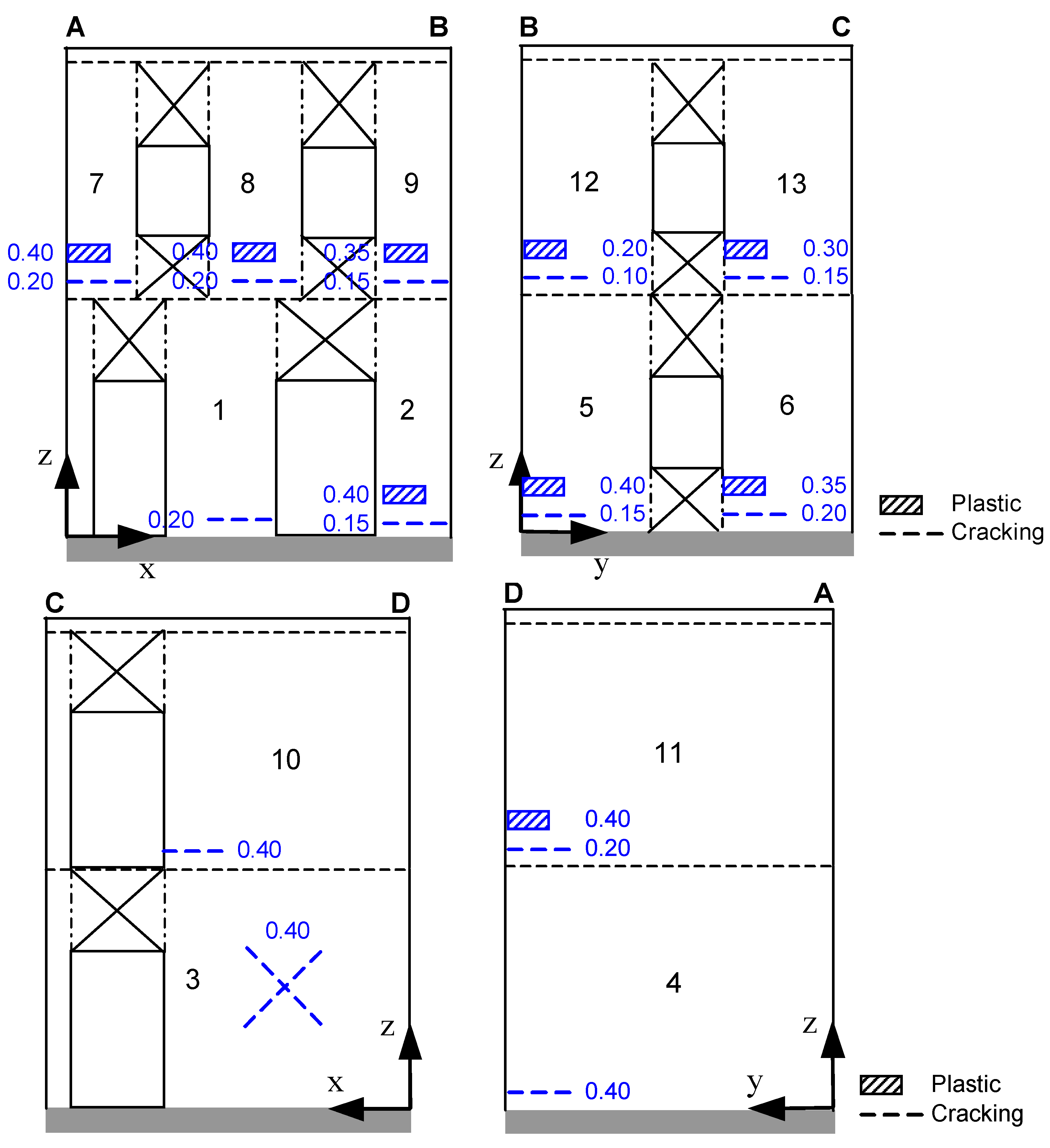
Figure 14 illustrates the damage progress in the masonry walls predicted by the ME model from a qualitative point of view. According to the constitutive equations, if the deformation in a pier reaches the value δcr or δmax (Figure 10), the pier is assumed to be in the “cracking state” or in the “plastic state”, respectively. Collapse occurs if the deformation reaches the limit value δu. The dead loads of the prototype are rather low, so the ME model predicts flexural failures for all of the masonry piers with the exception of Pier 3 (Figure 11), where a shear failure is always predicted.
During the first two shocks (nominal PGA = 0.05 and 0.10 g), no appreciable damage is detected, and the model response is almost linear elastic. The first damages appear during the third shock (nominal PGA = 0.15 g), when in-plane cracking occurs in Piers 5, 12 and 13 in the y direction and in Piers 2 and 9 in the x direction. This indicates that the first damages are concentrated along Corner B between the walls AB and CB. In the subsequent two shocks (PGA = 0.20 and 0.25 g), the largest parts of the piers crack, especially those of the second level: {1, 2, 7, 8, 9, 12, 13} in the x direction, and {5, 6, 8, 9, 11, 12, 13} in the y direction. Some piers crack with out-of-plane deformation. In addition, the deformation of Pier 12 goes beyond δmax in the plastic state.
During the shock with nominal PGA = 0.30 g, the same trend is observed, and also, Pier 13 reaches the plastic state. This indicates the beginning of a flexural failure mode on the second level of the building in the y direction. With the shock with PGA = 0.35 g, also Piers 6 and 9 reach the plastic state. Finally, in the last shock (PGA = 0.40 g), Piers 7 and 8 together with 2, 5 and 11 reach the plastic state. In all of the simulations, the deformations never reach the ultimate value δu, denoting that the ME model predicts additional capacity reserve.
Overall, the ME model predicts the collapse of the second level under a shock with a nominal PGA greater than 0.40 g, with main deformations in the y direction. This can be explained taking into account the warping of the timber floors. They are sustained by the walls parallel to the x direction, and the orthogonal walls have low compressive stress and low shear strength. The piers collapse in flexure in their plane; hence, the model predicts the failure of the second level with a II mode mechanism. This disagrees with the failure mode of the prototype detected during the experimental tests, characterized by the development of main cracks along the corners up to the overturning of the walls of the second level. Due to the assumption of rigid diaphragms, this collapse configuration cannot be correctly reproduced by the ME model.
Figure 14. Damage progress obtained by the ME model.
Buildings 05 00597 g014
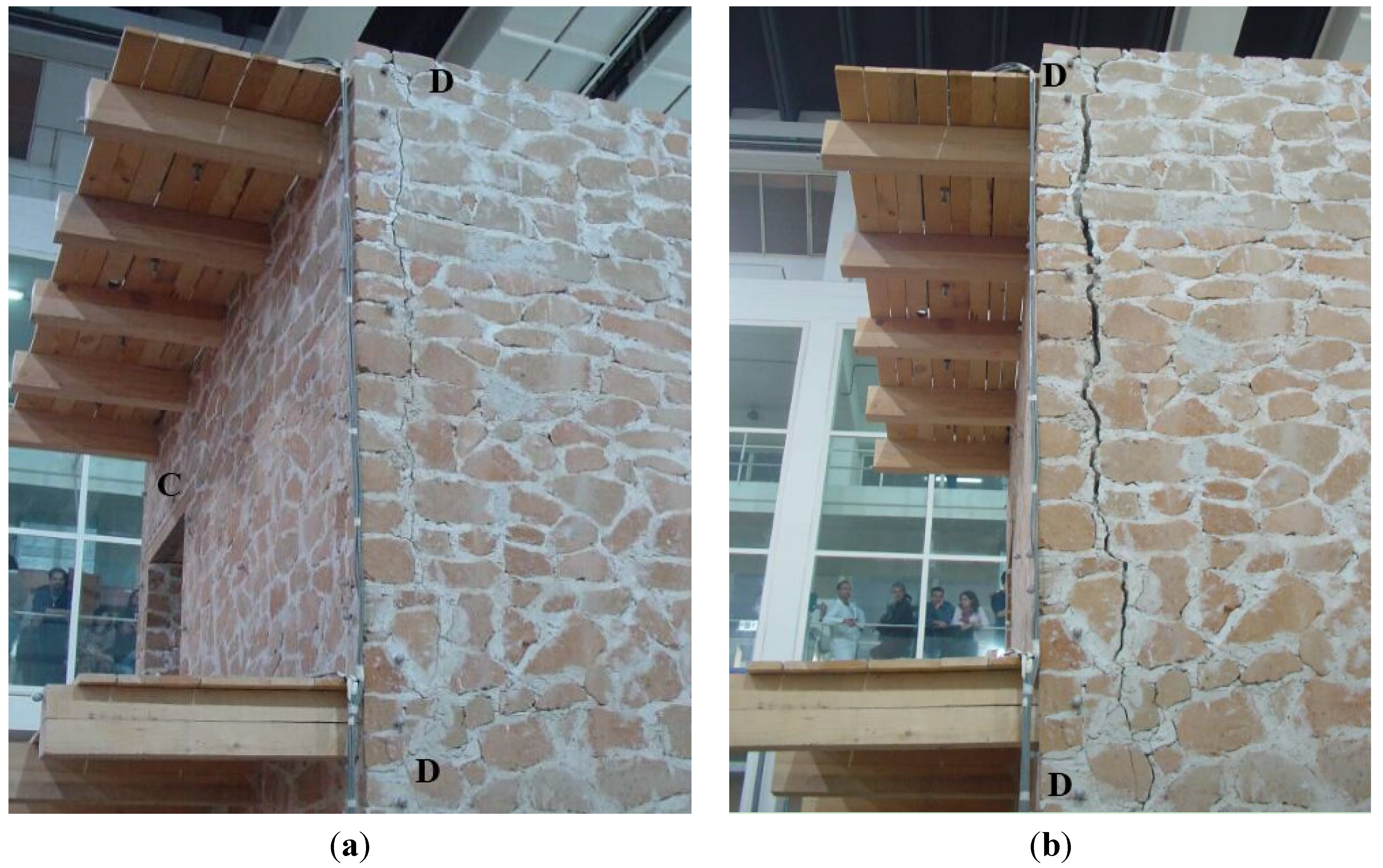
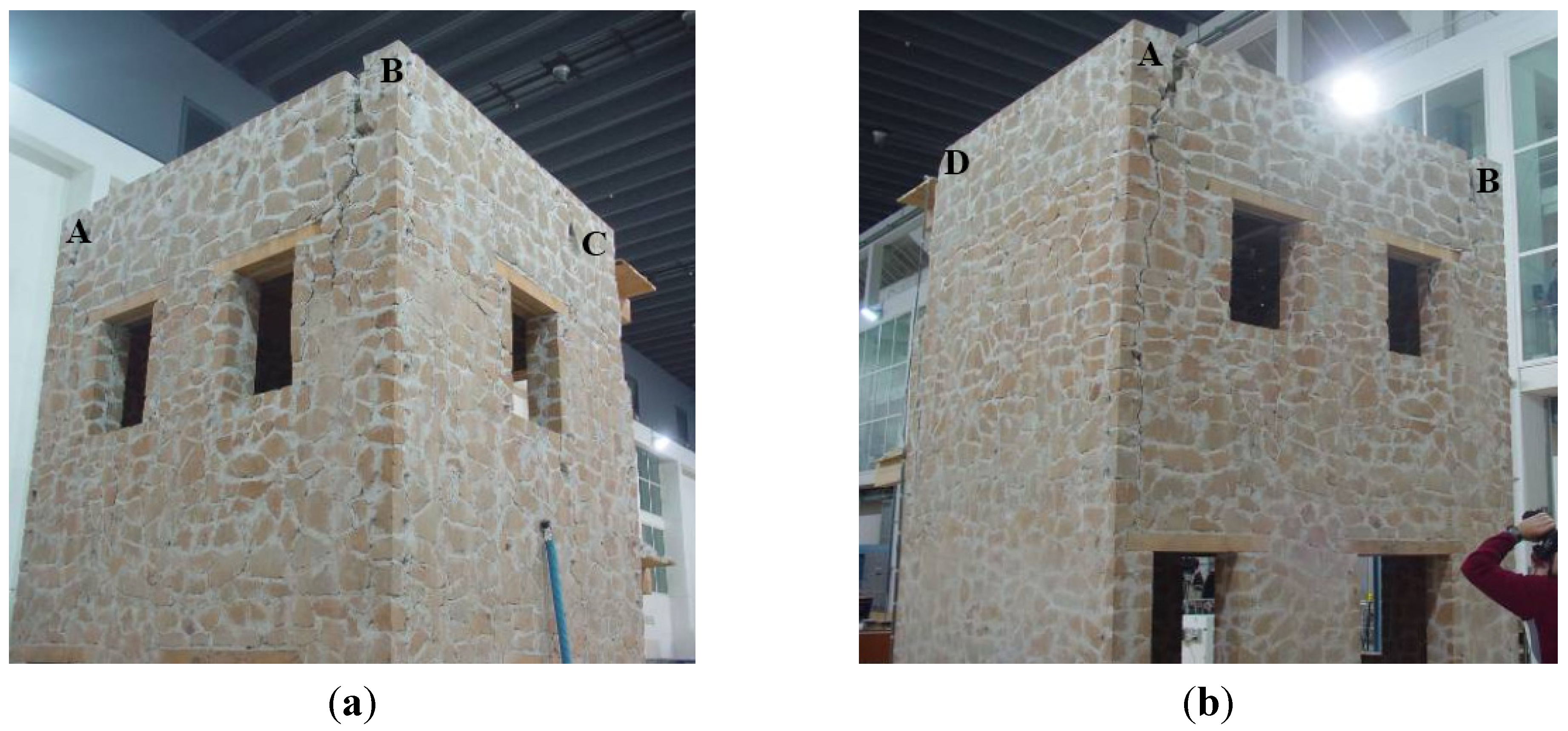
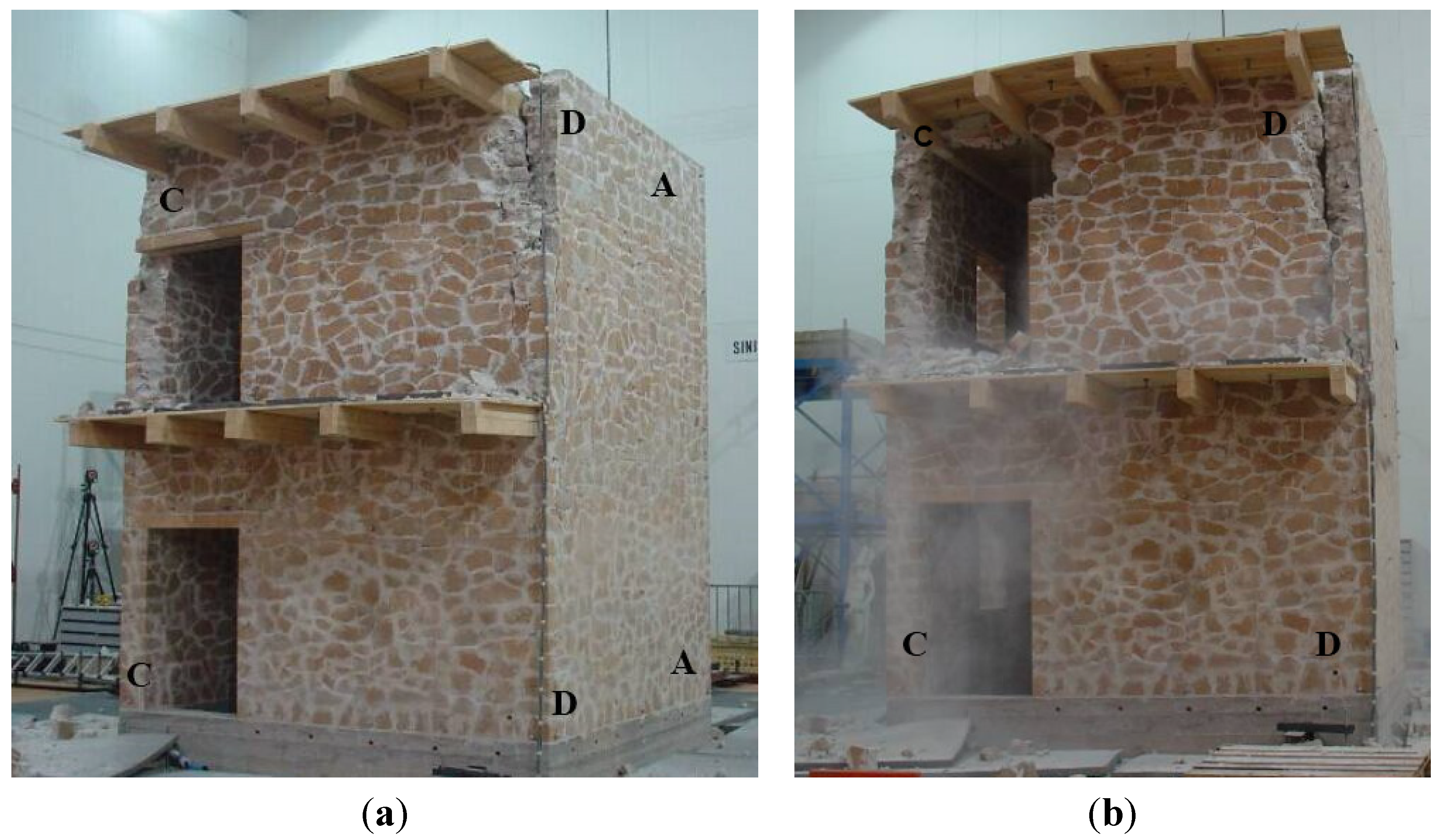
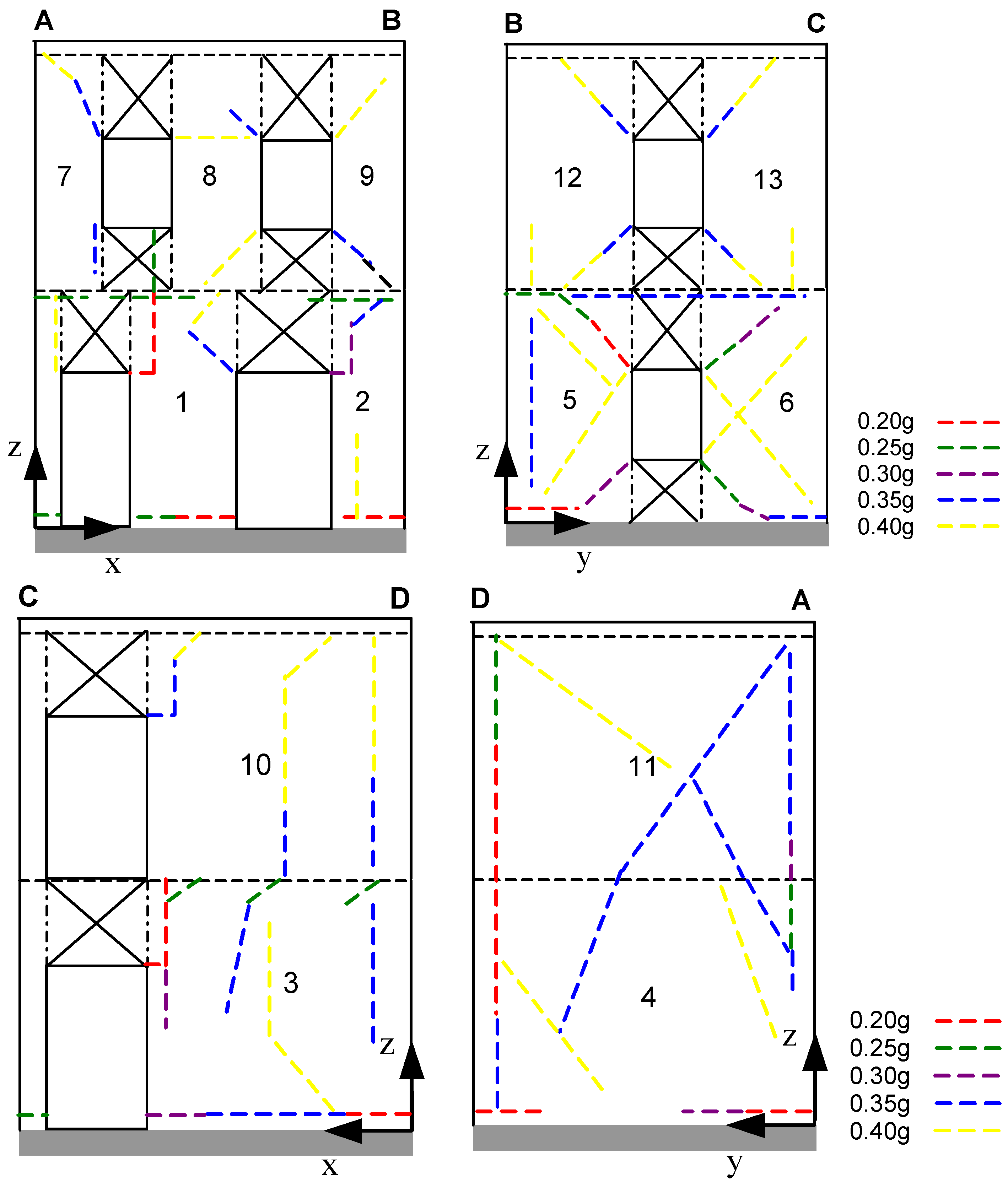
The FE model provides a linear response with the shocks with nominal PGA of 0.05 and 0.10 g, and an almost linear response under the shock with nominal PGA of 0.15 g. The first noticeable damages appear during the shock with nominal PGA equal to 0.20 g, when a main vertical crack develops along Corner D starting from the level of the first floor (as in the experiments; Figure 5). Other horizontal cracks appear at the base of the building (Façade AB) in the contact zone with the RC basement. In the subsequent analysis, the previous cracking pattern becomes wider, and a further main diagonal crack develops on the first level (Façade BC) starting from the corner of the window. The analysis with nominal PGA = 0.30 g confirms the previous trend, and in addition, a second main diagonal crack appears on the façade BC in which the typical cracking pattern with the “×” profile is recognized. At the same time, another vertical crack develops along Corner A. In the analysis with nominal PGA = 0.35 g, a diagonal crack develops on the façade DA, on both levels, and the vertical crack along Corners A and D increases. During the shock with PGA = 0.40 g, at 5.87 s, the numerical analysis stops due to the non-convergence of the solution (numerical collapse of the model). Displacements reach high values, and the cracking pattern confirms the previous trend.
The progress of the cracks, for all of the analyses, is summarized in Figure 15.
Figure 15. Damage progress obtained by the FE model.
Buildings 05 00597 g015
As a general remark, the FE model substantially matches the experimental collapse mode, reproducing the larger part of the damages. In addition, the phenomenon of opening of the corners is reasonably well reproduced.
A further comparison of the dynamic responses obtained through the two approaches is made analyzing the same parameters discussed in the previous section. Stiffness decay is shown in Figure 13. The ME model predicts a noticeable decay of the secant stiffness in the analyses with nominal PGA from 0.10 to 0.20 g, in both directions and for both levels of the building. The ME model response, in fact, is very sensitive to the cracking of the first pier (each pier is modelled as a single macro-element). In the subsequent shocks the stiffness continues to decrease, although with less evidence. In particular, stiffness decay is predominant at the second level in the y direction, where a stiffness reduction equal to about ten-times the initial elastic value is observed.
The evolution predicted by the FE model is different. The stiffness of the second level remains almost the same up to the shock with nominal PGA = 0.35 g, when a sudden decrease occurs. The stiffness of the base level gradually decreases starting from the shocks with nominal PGA = 0.30 g (x direction) and 0.15 g (y direction), until it reaches the same values predicted by the ME model. The premature stiffness decay predicted by the ME model with respect to the FE model is outlined also by the maximum base shears (Figure 13). 
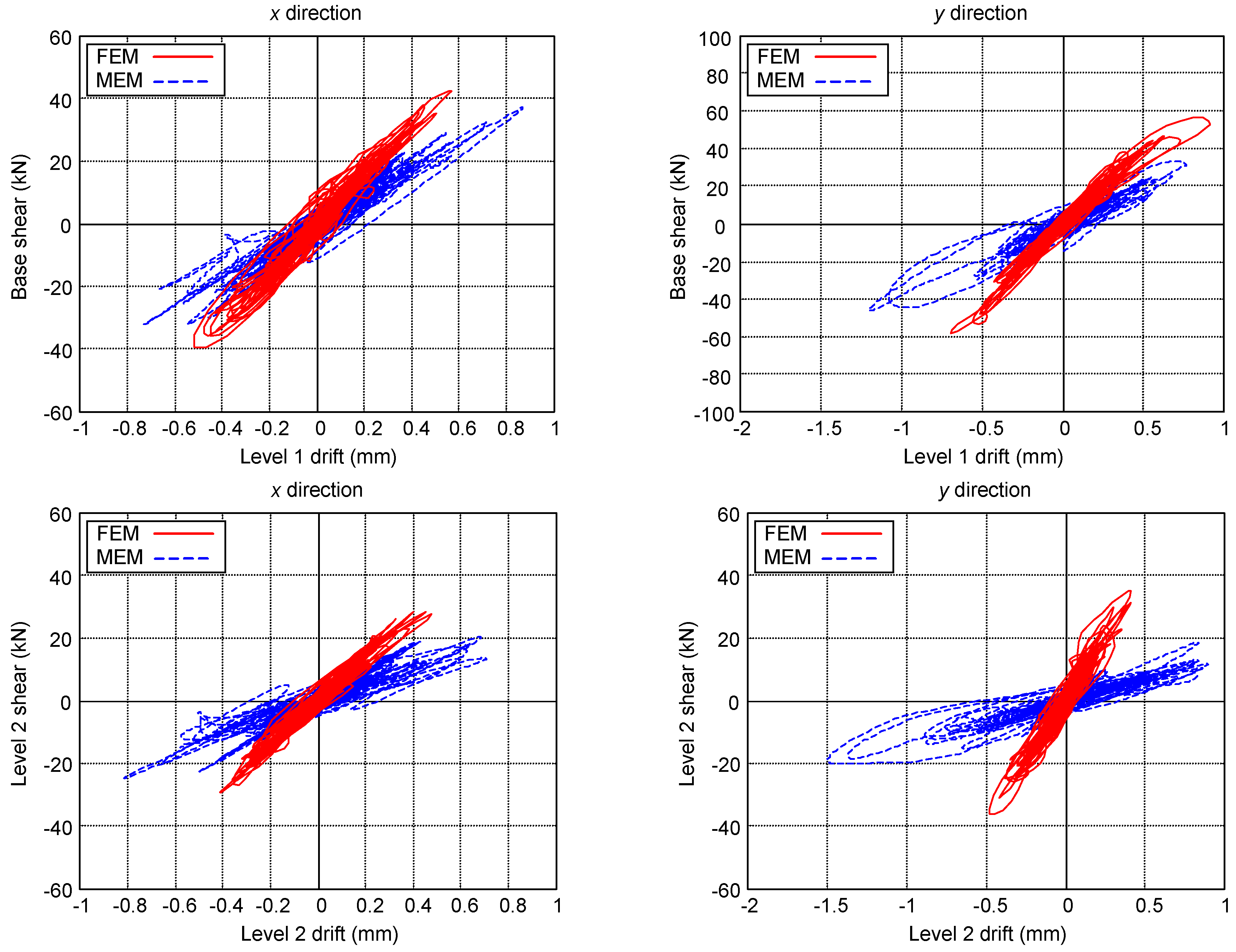
Figure 16 plots the shear forces vs. the corresponding drifts, comparing the responses obtained with the non-linear analyses with nominal PGA = 0.30 g. The differences between the two models are clearly visible.
Figure 16. Shear forces vs. corresponding drifts for the analyses with nominal PGA = 0.30 g.
Buildings 05 00597 g016
Responses in terms of displacements and accelerations are less significant for non-linear analyses. As reported before, the ME model provides higher values of displacements than the FE model. The errors Ed are significant: for example, at the second level, errors are detected up to 58.8% and 85% in the x and y directions, respectively (Table 6). On the contrary, for the shocks with PGA greater than 0.20 g, the absolute accelerations of the second level predicted by the ME model are lower than those obtained by the FE model (with errors Ea up to 36.4% and 47% in the two directions; Table 6).
Table 6. Percentage errors (non-linear analyses).
FloorDisplacements Ed (%)Accelerations Ea (%)
0.2 g0.3 g0.4 g0.2 g0.3 g0.4 g
F1x22.741.429.03.07.2−26.9
F1y63.454.9−22.432.325.1−27.2
F2x23.050.758.8−21.0−21.1−36.4
F2y70.485.041.00.6−13.7−47.0
The errors EV and EK are summarized in Table 7. These differences are confirmed by the spectral analysis of the signals. The dominant frequencies obtained with the FE model are higher than those obtained by the ME model, with differences increasing as the PGA increases. Analyzing the displacements, the errors on the dominant frequency, Efrd, range from 20% to 50%, while for accelerations the same errors vary from 20% to 80%.
As an example, Figure 17 shows the displacements amplitude spectra of the second floor for the simulations with nominal PGA = 0.30 g (linear and non-linear analyses, x and y directions). The spectra were obtained by a standard fast Fourier transform (FFT) procedure, operating on subsequent temporal windows with an overlap of 50%. The good agreement obtained with the linear models and the differences predicted by the non-linear ones are evident.
Table 7. Percentage errors (non-linear analyses).
LevelShear Forces EV (%)Stiffness EK (%)
0.2 g0.3 g0.4 g0.2 g0.3 g0.4 g
F1x−18.3−12.924.2−48.7−38.0−17.1
F1y−22.5−20.6−36.0−50.0−34.1−19.2
F2x−28.4−14.52.4−61.8−67.3−59.4
F2y−33.1−45.1−56.9−72.6−82.3−89.7
Figure 17. Displacement amplitude spectra of the second floor for linear and non-linear analyses with nominal PGA = 0.30 g.
Buildings 05 00597 g017
In general, even if both models predict a collapse PGA value equal to or greater than 0.40 g, they provide different collapse modes. This is substantially due to the differences in the modelling hypotheses between ME and FE approaches. Smeared cracking produces many and distributed cracks that result in a small, but constant stiffness decrease as the PGA increases (as observed during the experimental tests). When the damage has spread over the entire building, a sudden loss of strength and stiffness occurs.
On the one hand, the comparison between the two codes shows that the FE model is capable of reproducing with great confidence the experimental results (progress, location and extent of the damaged portions until collapse). The macro-element model, due to the intrinsic hypothesis of rigid floors, is capable of predicting the collapse load, but not providing a satisfactory reconstruction of the actual collapse mechanism (wall overturning due to the flexibility of the wooden floors). On the other hand, the results highlight that each model has a range of validity, which needs to be carefully understood, and the use of such tools requires high expertise. With respect, for instance, to the floor modelling, it is confirmed that different assumptions on the diaphragms’ stiffness significantly affect the building overall seismic response. In fact, in the case of flexible floors (like in the FE models), there is no load transfer from collapsed walls to still efficient structural elements. On the contrary, in the case of stiff floors (like in the ME models), the load transfer is overestimated, producing, in turn, an overestimation of the building seismic capacity. In this respect, the results of the macro-element model, despite its intrinsic simplifications, should be considered as an upper limit of the building capacity, which can be reached only when the out-of-plane and the local damage mechanisms are not previously activated.

5. Conclusive Remarks

The paper reported a comparison between two numerical models used to investigate the seismic behavior of existing masonry buildings. As a reference case study, an unreinforced masonry prototype with flexible diaphragms tested on a shaking table until collapse was considered. The first numerical model was built by the finite element method through a macro-model technique; the second one was built by using a macro-element approach through the implementation of a non-linear algorithm in the MATLAB tool.
The models adopt different mechanical hypotheses to account for the non-linear behavior of the masonry and different techniques to reproduce the building geometry. The two procedures were employed to simulate the tests, by linear and non-linear time-history analyses. The comparison was performed considering the displacements and the absolute accelerations, as these are two of the most significant global kinematic parameters that synthesize the dynamic response of a building. In addition, the shear forces, the stiffness decay and the damage evolution were also considered, as parameters with significant engineering relevance.
The results highlighted that the FE model is capable of reproducing with good confidence the experimental damages, while the macro-element model, due to the intrinsic hypothesis of rigid floors, is capable of predicting the collapse load, but not providing a satisfactory reconstruction of the actual collapse mechanism. Errors on displacements and accelerations are acceptable in the simulations with low-to-moderate PGA intensities, i.e., in the almost linear range of the dynamic response. In all of the simulations, the ME model underestimates the shear forces, since it provides a more pronounced stiffness decay with respect to the FE model.
As the availability of an effective non-linear tool for the seismic assessment of masonry structural elements is still a crucial requirement, the paper suggests that the seismic analysis of traditional masonry buildings (with flexible floors and poor connections between the walls) should be examined through a cross-numerical approach.

Acknowledgments

This research was developed in the framework of the ReLUIS-DPC project (Line 1: “Assessment and reduction of the vulnerability of masonry buildings”) funded by the Italian Department of Civil Protection.

Author Contributions

All the authors contributed equally to this paper.

Conflicts of Interest

The authors declare no conflict of interest.

References

  1. D’Ayala, D.; Paganoni, S. Assessment and analysis of damage in L’Aquila historic city centre after 6th April 2009. Bull. Earthq. Eng. 2011, 9, 81–104. [Google Scholar] [CrossRef]
  2. Penna, A. Seismic assessment of existing and strengthened stone-masonry buildings: Critical issues and possible strategies. Bull. Earthq. Eng. 2015, 13, 1051–1071. [Google Scholar] [CrossRef]
  3. Lourenço, P.B.; Mendes, N.; Ramos, L.F.; Oliveira, D.V. Analysis of masonry structures without box behavior. Int. J. Archit. Herit. 2011, 5, 369–382. [Google Scholar] [CrossRef] [Green Version]
  4. Diaferio, M.; Foti, D.; Giannoccaro, N.I.; Ivorra, S. Optimal model through identified frequencies of a masonry building structure with wooden floors. Int. J. Mech. 2014, 8, 282–288. [Google Scholar]
  5. Kappos, A.J.; Penelis, G.G.; Drakopoulos, C.G. Evaluation of simplified models for lateral load analysis of unreinforced masonry buildings. ASCE J. Struct. Eng. 2002, 128, 890–897. [Google Scholar] [CrossRef]
  6. Casolo, S.; Uva, G. Nonlinear analysis of out-of-plane masonry façades: Full dynamic vs. pushover methods by rigid body and spring model. Earthq. Eng. Struct. Dyn. 2013, 42, 499–521. [Google Scholar] [CrossRef]
  7. Vamvatsikos, D.; Cornell, C.A. Direct estimation of the seismic demand and capacity of oscillators with multi-linear static pushovers through IDA. Earthq. Eng. Struct. Dyn. 2006, 35, 1097–1117. [Google Scholar] [CrossRef]
  8. Galasco, A.; Lagomarsino, S.; Penna, A. On the Use of Pushover Analysis for Existing Masonry Buildings. In Proceedings of the 13th European Conference on Earthquake Engineering, Geneva, Switzerland, 3–8 September 2006.
  9. Casolo, S.; Uva, G. Full Dynamic and Pushover Analyses of Out-of-Plane Masonry Facades: Application and Comparisons by RBSM. In Proceedings of the 14th World Conference on Earthquake Engineering, Beijing, China, 12–17 October 2008.
  10. Bartoli, G.; Betti, M. Cappella dei principi in Firenze, Italy: Experimental analyses and numerical modeling for the investigation of a local failure. ASCE J. Perform. Constr. Facil. 2013, 27, 4–26. [Google Scholar] [CrossRef]
  11. Betti, M.; Galano, L. Seismic analysis of historic masonry buildings: The vicarious palace in Pescia (Italy). Buildings 2012, 2, 63–82. [Google Scholar] [CrossRef]
  12. Caliò, I.; Marletta, M.; Pantò, B. A new discrete element model for the evaluation of the seismic behaviour of unreinforced masonry buildings. Eng. Struct. 2012, 40, 327–338. [Google Scholar] [CrossRef]
  13. Magenes, G.; Della Fontana, S. Simplified Non-Linear Seismic Analysis of Masonry Buildings. In Proceedings of the 5th International Masonry Conference, London, UK, 13 July 1998.
  14. Bucchi, F.; Arangio, S.; Bontempi, F. Seismic Assessment of an Historical Masonry Building using Nonlinear Static Analysis. In Proceedings of the 14th International Conference on Civil, Structural and Environmental Engineering Computing, Sardinia, Italy, 3–6 September 2013.
  15. Lagomarsino, S.; Penna, A.; Galasco, A.; Cattari, S. TREMURI program: An equivalent frame model for the nonlinear seismic analysis of masonry buildings. Eng. Struct. 2013, 56, 1787–1799. [Google Scholar] [CrossRef]
  16. ANSYS, v.11.0; ANSYS Manual Set; ANSYS Inc.: Canonsburg, PA, USA, 1998.
  17. Galano, L.; Selleri, F. Analisi sismica degli edifici in muratura: Un modello semplificato a macroelementi. Ing. Sismica 2004, 21, 28–45. (In Italian) [Google Scholar]
  18. Betti, M.; Galano, L.; Vignoli, A. Comparative analysis on the seismic behaviour of unreinforced masonry buildings with flexible diaphragms. Eng. Struct. 2014, 61, 195–208. [Google Scholar] [CrossRef]
  19. De Canio, G.; Dolce, M.; Goretti, A.; Marnetto, R. Progetto TREMA–Tecnologie per la Riduzione degli Effetti sismici sui Manufatti Architettonici in muratura e in ca. MURST Legge n. 449/1997, D.M. 10 Maggio 2000. (In Italian)
  20. Dolce, M.; Ponzo, F.C.; di Croce, M.; Moroni, C.; Giordano, F.; Nigro, D.; Marnetto, R. Experimental Assessment of the CAM and DIS-CAM Systems for the Seismic Upgrading of Monumental Masonry Buildings. In Proceedings of the 1st International Conference on Protection of Historical Constructions, Rome, Italy, 26–28 October 2009.
  21. Dolce, M.; Ponzo, F.C.; Moroni, C.; Nigro, D.; Goretti, A.; Giordano, F.; de Canio, G.; Marnetto, R. 3D Dynamic Tests on 2/3 Scale Masonry Buildings Retrofitted with Different Systems. In Proceedings of the 14th World Conference on Earthquake Engineering, Beijing, China, 12–17 October 2008.
  22. De Vekey, R.C.; Sassu, M. Comparison on Non-destructive In-Situ Mechanical Tests on Masonry Mortars: The PNT-G Method and the Helix Method. In Proceedings of the 11th International Brick/Block Masonry Conference, Shanghai, China, 14–16 October 1997.
  23. Sahlin, V. Structural Masonry; Prentice-Hall: Englewood Cliffs, NJ, USA, 1971. [Google Scholar]
  24. Galano, L.; Vignoli, A. Resistenza a taglio di murature di pietrame: Analisi comparata della rappresentatività di tipiche prove di taglio in situ. In Atti del X Congresso Nazionale ANIDIS L’Ingegneria Sismica in Italia, Potenza-Matera, Italia, 9–13 settembre 2001. (In Italian)
  25. Magliulo, G.; Petrone, C.; Capozzi, V.; Maddaloni, G.; Lopez, P.; Manfredi, G. Seismic performance evaluation of plasterboard partitions via shake table tests. Bull. Earthq. Eng. 2014, 12, 1657–1677. [Google Scholar] [CrossRef]
  26. Giamundo, V.; Lignola, G.P.; Maddaloni, G.; Balsamo, A.; Prota, A.; Manfredi, G. Experimental investigation of the seismic performances of IMG reinforcement on curved masonry elements. Comp. Part B Eng. 2015, 70, 53–63. [Google Scholar] [CrossRef]
  27. Avossa, A.M.; Malangone, P. Seismic performance assessment of masonry structures with a modified “concrete” model. Bull. Earthq. Eng. 2015. [Google Scholar] [CrossRef]
  28. Betti, M.; Vignoli, A. Numerical assessment of the static and seismic behaviour of the basilica of Santa Maria all’Impruneta (Italy). Constr. Build. Mater. 2011, 25, 4308–4324. [Google Scholar] [CrossRef]
  29. Calderini, C.; Cattari, S.; Lagomarsino, S. The use of the diagonal compression test to identify the shear mechanical parameters of masonry. Constr. Build. Mater. 2010, 24, 677–685. [Google Scholar] [CrossRef]
  30. Elmenshawi, A.; Sorour, M.; Mufti, A.; Jaeger, L.G.; Shrive, N. Damping mechanisms and damping ratios in vibrating unreinforced stone masonry. Eng. Struct. 2010, 32, 3269–3278. [Google Scholar] [CrossRef]

