Simulating Performance Risk for Lighting Retrofit Decisions

Abstract

In building retrofit projects, dynamic simulations are performed to simulate building performance. Uncertainty may negatively affect model calibration and predicted lighting energy savings, which increases the chance of default on performance-based contracts. Therefore, the aim of this paper is to develop a simulation-based method that can analyze lighting performance risk in lighting retrofit decisions. The model uses a surrogate model, which is constructed by adaptively selecting sample points and generating approximation surfaces with fast computing time. The surrogate model is a replacement of the computation intensive process. A statistical method is developed to generate extreme weather profile based on the 20-year historical weather data. A stochastic occupancy model was created using actual occupancy data to generate realistic occupancy patterns. Energy usage of lighting, and heating, ventilation, and air conditioning (HVAC) is simulated using EnergyPlus. The method can evaluate the influence of different risk factors (e.g., variation of luminaire input wattage, varying weather conditions) on lighting and HVAC energy consumption and lighting electricity demand. Probability distributions are generated to quantify the risk values. A case study was conducted to demonstrate and validate the methods. The surrogate model is a good solution for quantifying the risk factors and probability distribution of the building performance.

1. Introduction

In a retrofit decision process, professionals perform energy audits and construct dynamic simulation models to benchmark the performance of existing buildings and predict the effect of retrofit interventions [1]. Retrofit decisions can be evaluated using multi-objective optimization [2,3]. However, deterministic models do not provide insights into underperforming risks associated with each retrofit intervention. A more reliable approach is performing sensitivity analysis to quantify the influence of different risk factors on building operation performance [4,5]. To do this, a distribution is chosen for a number of inputs and numerous models are generated to simulate and determine statistics of important outputs. For instance, sensitivity analysis for thermal parameter ranking can help to choose the envelope material type.

A number of researchers have studied uncertainty and sensitivity analysis in building design and retrofit decisions. For example, Eisenhower et al. [6] used EnergyPlus to perform uncertainty analysis with one thousand uncertain parameters (almost all numeric parameters in the EnergyPlus input file were included, except those parameters such as architectural parameters and text-based parameters), and quantified which intermediate processes were contributing the most to this uncertainty using a decomposition-based approach. Shen et al. [7,8] studied lighting control strategies using different parameters such as climate zones, blind type and window-to-wall ratios. The combination of only a few parameters can result in a large number of building models. The number of simulations significantly increases when more parameters are evaluated. Heo et al. [1] used Bayesian calibration of normative energy models for energy model calibration in retrofit projects. However, the normative energy model is essentially lightweight formulations of heat balance equations, resulting in limitations compared to the advanced energy modeling available in programs such as EnergyPlus.

Two main problems occur when using uncertainty and sensitivity analysis to evaluate a building retrofit decision. The first problem is the long simulation times, especially when large numbers of simulations are needed. Sensitivity analysis requires performing energy and lighting simulations using advanced tools such as EnergyPlus [9], Radiance, and Daysim [10,11]. The current workflow of sensitivity analysis [4] shows that a large number of simulations may have to be performed [11]. In addition, when the variation of input parameters becomes significant, this results in a large number of simulations requiring a long time to complete the analysis. Therefore, two solutions were proposed to solve this problem. The first solution is to develop new models that run faster. For example, Hu and Olbina [12] developed an analytical model to simulate the day-lighting performance of blinds with different blind reflectance and glazing transmittances. The model can quickly predict the interior luminance without repeatedly simulating all the possible parameters. A neural network model was also developed to predict the luminance and building energy by reducing the simulation complexity [13,14]. An expert system can provide realistic results using prior knowledge from lighting designers and simulation data [15,16]. The second solution is to reduce the number of simulations. Instead of sampling parameters in the whole space, the samples can be reduced by intelligently selecting optimum positions. For example, a surrogate model uses adaptive sampling to select sample points with maximization of errors. The surrogate model treats the computationally expensive simulation code as a data generating black-box, only taking into account its input-output behavior and constructing approximation models. The approximation surface of the surrogate model can be constructed using a small sample size of simulation data. Once the surrogate model is developed, the input variables can be directly fed into the surrogate model to generate the output values (i.e., energy consumption).

The second problem is identifying critical risk factors and sampling these factors efficiently. Some risk factors tend to be ignored or simulated inappropriately because these parameters are not scalar and distribution functions are not clearly defined. For example, the sky model or weather conditions affect the indoor daylight levels, directly affecting daylight sensor readings or indirectly affecting human control behavior. The sky model has been recognized as the key factor in lighting and energy simulation. The sky model is generated from a weather file whose data are measured from a weather station. A weather file contains many meteorological variables where radiation and temperature are typically the most important factors. Currently, most methods focus on temperature only [17]. In lighting simulation, other parameters such as global and solar radiation and sky clearness have more weight than temperature. Therefore, the weather data should be further analyzed when used in lighting retrofit projects. Another essential parameter for lighting and energy simulation is the occupancy pattern, which affects occupant control behavior and internal heat generation. When occupancy based control is used for lighting, occupancy will directly influence the lighting on/off status [12,18]. The third parameter is lighting control strategy. Different control strategies significantly affect building energy, especially lighting energy consumption [8]. For example, significant savings can be achieved in lighting energy consumption using integrated closed-loop blind and lighting control strategy.

Therefore, based on the problems identified in the analysis of lighting retrofit projects, the aim of this research is to develop a surrogate model to quantify the influence of risk factors (i.e., weather condition, occupancy pattern, and lighting control strategy) on building performance (i.e., HVAC/lighting energy savings, and lighting demand).

2. Model Development

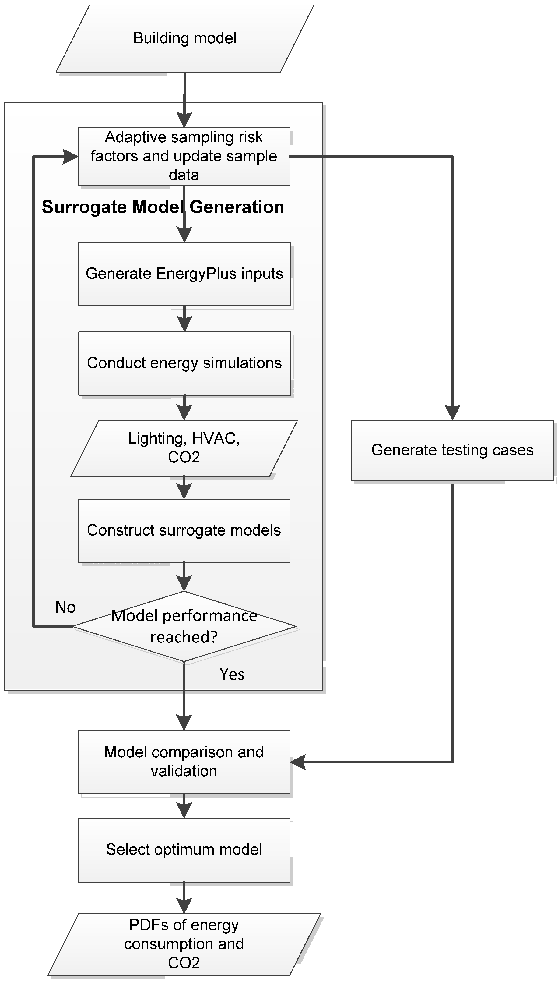
2.1. Model Structure

A surrogate model is used to predict energy consumption and lighting electricity demand. The surrogate model uses adaptive sampling to reduce the difference between the surrogate model and simulation model [19]. For this sampling technique, the sampling position in current iteration is determined by the previous iteration. For example, in Figure 1, in the first iteration, the predicted value at point A has a large deviation from the simulation model even though the sample points (white dots) have a small error. In the next iteration, a new sample point is added at position A, having a maximum error (i.e., the largest vertical distance between the curve of the simulation model and the surrogate model). In this way, new sample points are calculated sequentially.

Figure 1. Adaptive sampling technique.

Figure 1. Adaptive sampling technique.

The model structure is shown in Figure 2. The input is a building model containing building thermal, location, and geometry data. The first step is sampling input variables (i.e., risk factors) using Latin hypercube sampling method. The input variables include occupancy level, weather, control strategy and luminaire type. Other parameters such as envelope thermal properties and surface reflectances are obtained from design drawings or on-site auditing.

Figure 2. Model structure.

Figure 2. Model structure.

In the next steps, shown in Figure 2, energy simulation is performed using EnergyPlus. The input file of EnergyPlus is automatically generated by incorporating risk factors into an input file template. The output of the energy simulation includes energy consumption, electricity demand, etc. Then, surrogate models can be built by using methods such as polynomial response surfaces, Kriging, support vector machines and neural networks. A preliminary test using a DOE reference office building located in Chicago was performed which showed that the neural network model generally provides better results than the other approaches, which is consistent with a previous study on energy consumption prediction using neural networks [20].

In the next two steps, the surrogate model is validated and the optimum one is selected. Mean square error (MSE) is a metric for measuring the model performance. The dataset is divided into training and testing datasets for validation. After the surrogate model is constructed, the input variables are sampled using the Monte Carlo method. A large number of combinations of the input variables are generated and fed into the surrogate model for energy consumption prediction. Then, probability distributions of lighting and heating, ventilation, and air conditioning (HVAC) energy consumption can be generated.

2.2. Risk Factor Sampling

The risk factors considered in this model include occupancy level, weather, luminaire input wattage, and lighting control strategy. The use case is to quantify the performance risks when a fluorescent luminaire is replaced by another more energy efficient luminaire and advanced lighting control system. This section will introduce how to sample the risk factors: occupancy level, lighting control strategies, and weather conditions.

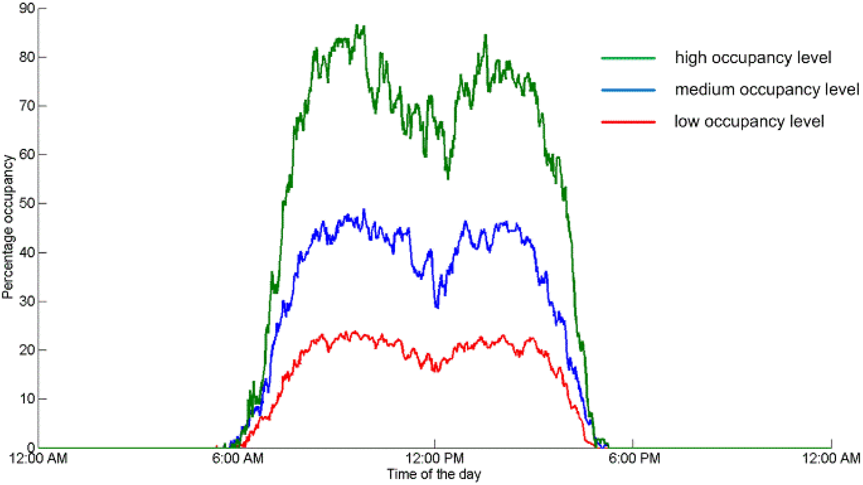
2.2.1. Occupancy Level

Occupancy patterns can be simulated (e.g., using occupancy model) or measured (e.g., onsite survey and audit). A stochastic occupancy model was developed using actual office data [8]. Occupancy data was monitored and logged every minute for nine offices over 42 weekdays and 18 weekend days. The model can be used to simulate the occupancy status for every occupant in the building. Each individual occupancy state is represented as a Markov Chain where the state transition probabilities are derived from the actual occupancy data. Figure 3 shows occupancy patterns (total occupancy) with three dynamic occupancy levels (low, medium, and high) calculated from the dynamic occupancy model. The occupants arrive around 7:00–9:00 a.m. and leave around 5:00–6:00 p.m.

Figure 3. An example of occupancy patterns according to three peak occupancy levels

Figure 3. An example of occupancy patterns according to three peak occupancy levels

2.2.2. Lighting Control Strategies

Three lighting control strategies are evaluated: manual control (or fixed schedule based control); dynamic occupancy based control, or occupancy + day-lighting control.

• Manual Control: The lights are turned on in compliance with a pre-defined schedule. There is no automation in this process. A retrofitted building often uses this control strategy.
• Occupancy Control: This control strategy controls lighting on/off status based on the presence of occupants. In building simulation, a dynamic occupancy model can generate occupancy patterns that are used to simulate the occupant presence.
• Occupancy and Day-Lighting Control: This control strategy uses occupancy sensors to detect occupant presence and uses daylight sensors to measure daylight. Lights in perimeter zones dim in response to the daylight sensor readings. It is expected that more energy savings can be achieved while still maintaining desired luminance levels.

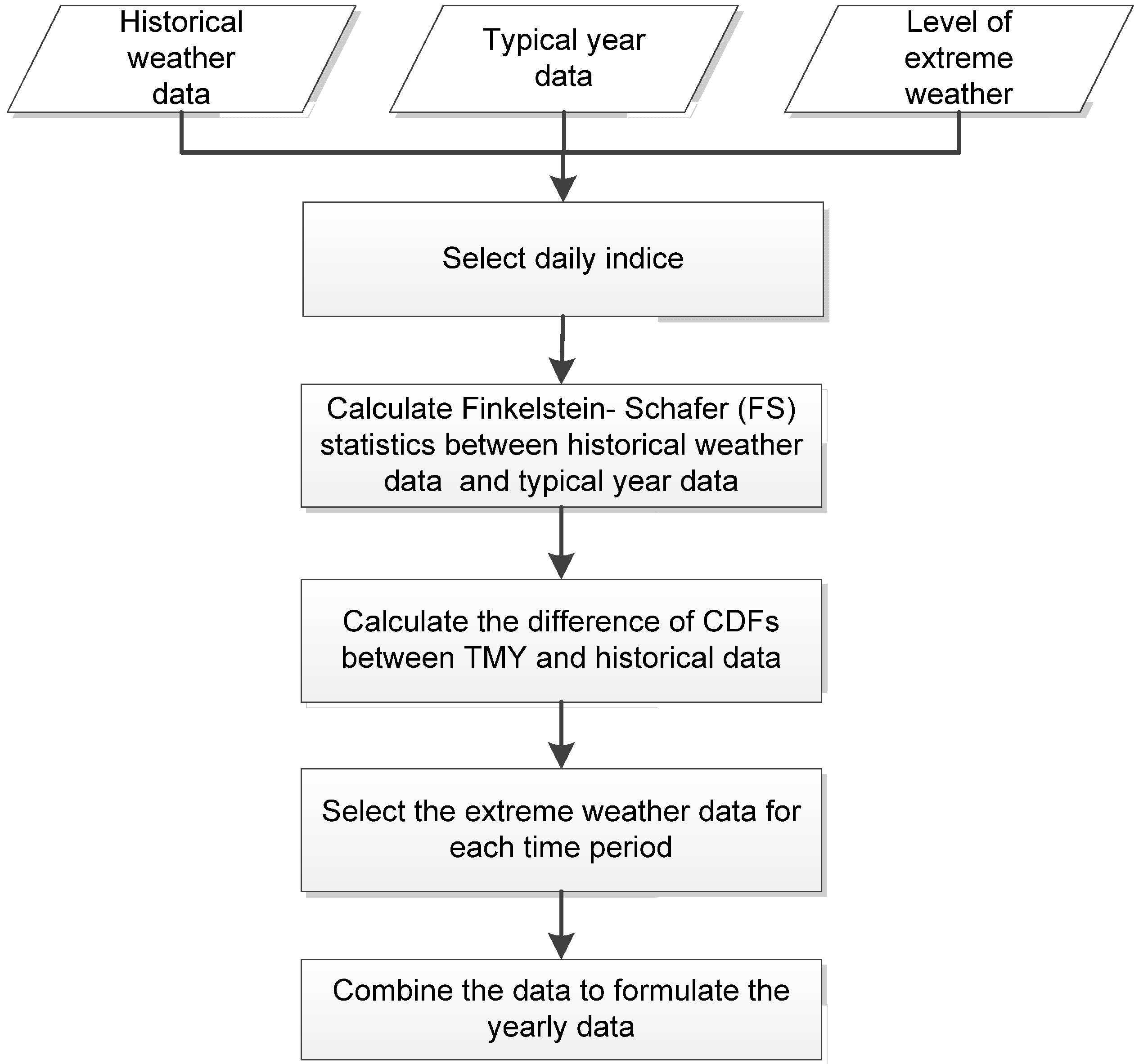
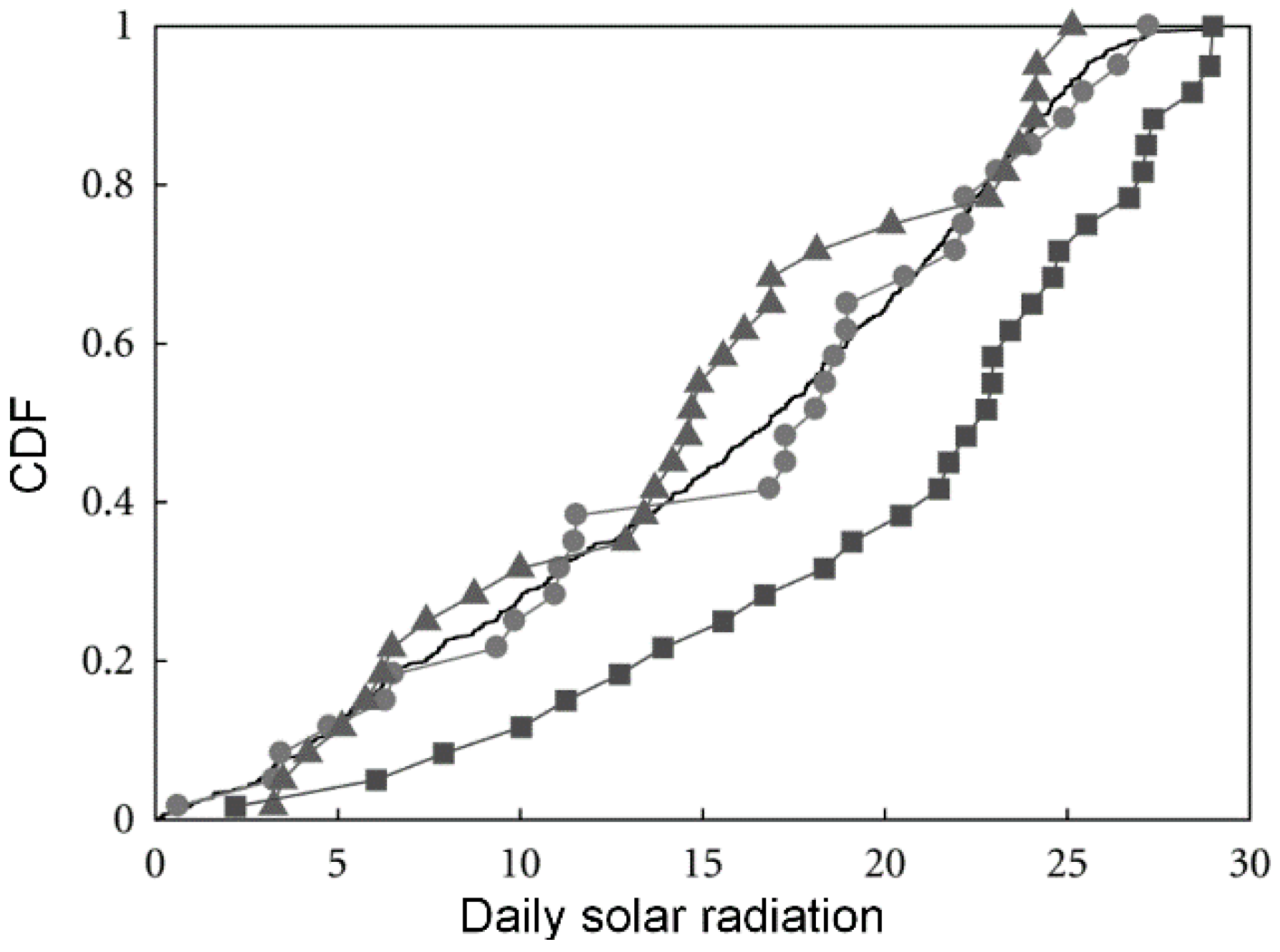
2.2.3. Weather Conditions

Sky clearness, solar radiation, and temperature affect HVAC and lighting energy consumption, especially when daylight control is used. In order to evaluate risks caused by variations in weather conditions, the meteorological data needs to be sampled. Previous research only sampled temperature in order to create a new weather file for energy simulation. This is inappropriate because sampling temperature alone fails to evaluate risks that influence lighting energy consumption. We developed a method to generate dynamic weather conditions relevant to lighting simulation using statistical analysis of historical weather data. This method is based on the Sandia method [21], which is an empirical approach that selects individual months from different years of the period of record to formulate a TMY weather file that is used in deterministic building simulations [22]. The weather files generated for our analysis represents extreme historical weather conditions based on probability analysis. These weather files are different from TMY weather files typically used for EnergyPlus simulations. Figure 4 shows the main steps of how to generate the dynamic weather files. The major steps are described as follows.

Figure 4. Flow chart of generating extreme weather data from historic weather data.

Figure 4. Flow chart of generating extreme weather data from historic weather data.

In the first step, the model input is defined. The historical weather data can be retrieved from the NREL website, which provides 20 years of actual weather data. TMY weather data are generated by processing historical weather data using the Sandia method. Data sources used in creating TMY data include the Typical Meteorological Year (TMY2, TMY3), and International Weather for Energy Calculation (IWEC) datasets. The input to the model is the level of extreme weather, where the level can be categorized into: (1) cloudy; (2) partially cloudy; and (3) clear. A Gaussian distribution is used for each level.

In the next step, the daily index such as clearness and solar radiation can be selected, depending on the simulation purpose. For example, when evaluating lighting energy, we use C = total radiation/diffuse radiation. Then a cloudy day would be represented by a small value of C. In order to generate a yearly weather file, statistical differences between historical data and typical data were quantified according to the Sandia method by calculating Finkelstein-Schafer (FS) statistics for relevant weather data. FS is defined in Equation (1).

$$\mathit{FS}=(1/n){\displaystyle \sum }_{i=1}^n{\text{δ}}_i$$

(1)

where ${\text{δ}}_i$ = absolute difference between the long-term cumulative probability functions (CDF) and the candidate month CDF at x_i, and n = the number of daily readings in a month.

In the next step, the differences between CDFs of typical year and CDFs of other years are calculated. The calculation can be done using histograms, similar to calculating the area between the two CDFs. Based on the calculated statistics, extreme weather is selected based on the CDF difference. For example, assume the weather data in January of 1995 has the largest CDF difference from the CDF of TMY data. Then this month data is selected for January when building the extreme cloudy year data. Note that different time periods may be used. For example, the time period may be weekly instead of monthly. Figure 5 shows an example of CDFs for global solar radiation. The whole year extreme weather data are created by combining the data calculated from each time period (e.g., month, week).

Figure 5. Cumulative Probability Functions (CDFs) of solar radiation in a month.

Figure 5. Cumulative Probability Functions (CDFs) of solar radiation in a month.

3. Case Study

In this case study, a lighting system retrofit is performed to reduce the power density from 13.83 W/m² (existing luminaire) to 11.52 W/m² (retrofit luminaire) and to add advanced lighting control strategies.

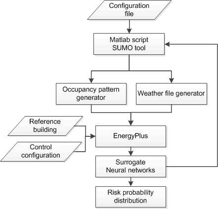
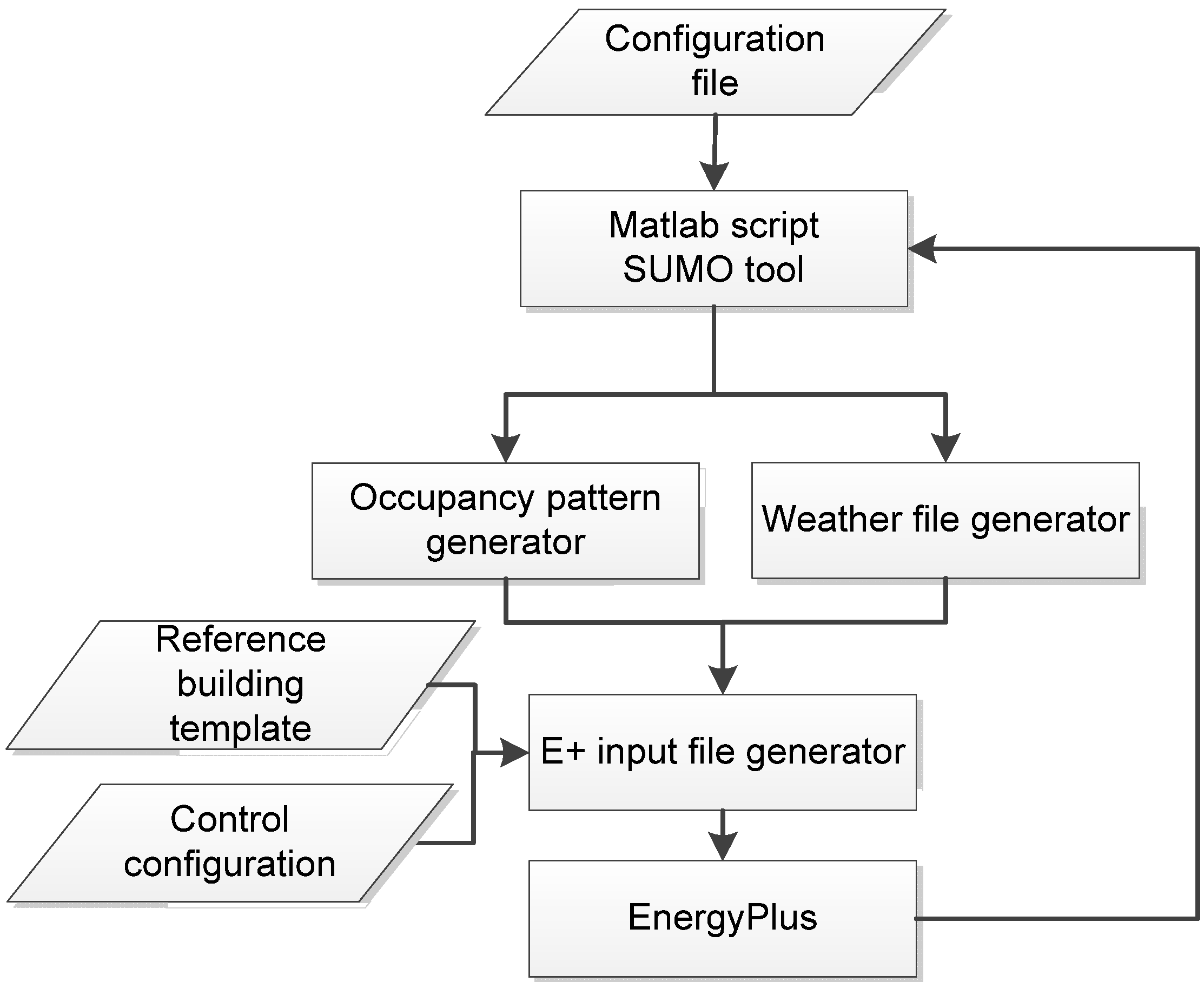
3.1. Model Implementation

The surrogate model is generated by using the SUrrogate MOdeling (SUMO) Toolbox [23], which is a Matlab toolbox that automatically builds accurate surrogate models (or response surface models) from a given data source (e.g., simulation code) within accuracy and time constraints. The toolbox minimizes the number of data points by selecting the best sample position adaptively and automatically, requiring no user input besides some initial configuration. In this case study, we used neural network model as the training model. The model was implemented as shown in Figure 6.

• Configuration File: This file defines the parameters of the surrogate model. For example, parameter of neural networks, and data sampling method (Latin hypercube sampling method) are used in this case study.
• Matlab Script/SUMO Tool: The tool calculates the objective function (i.e., lighting and HVAC energy consumption) from the output of EnergyPlus simulation. In the meantime, the tool calls the data generator to generate the sample for the next round simulation.
• Weather File Generator: Implemented in Python, it can dynamically produce the weather file by combing monthly actual weather data, given the probability from Matlab script.
• Occupancy Pattern Generator: Implemented in Matlab, it uses the stochastic occupancy model developed from collected office data [8].
• EnergyPlus Input File Generator: Implemented in Python, it reads risk factors, the reference building model template, and the control configuration file. The control configuration file defines the control strategy readable by EnergyPlus. The reference building model is modified from U.S. DOE reference model.
• EnergyPlus: In each iteration of the surrogate modeling process, the complete input file is fed into EnergyPlus. Parallel simulation uses a total of eight threads. The output file is processed by the SUMO tool.

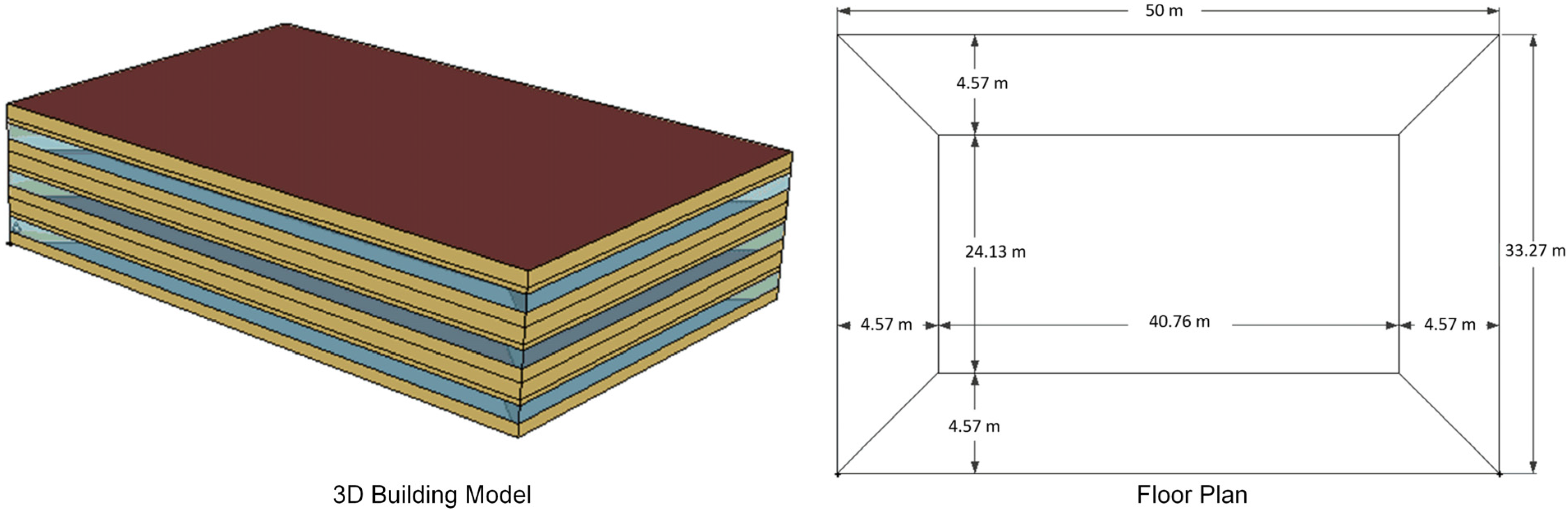
Figure 6. Structure of the implementation method.

Figure 6. Structure of the implementation method.

3.2. Building Model

The US DOE commercial reference model for medium office building (post 1980 building) is selected as the retrofit building for this case study [24]. The building is located in Chicago, IL and has three floors. Each floor has four perimeter zones and a core zone (see Figure 7). The main building parameters are:

• Envelope: The envelope thermal properties comply with ASHRAE Standard 90.1-1989 [25]. The exterior wall is set to steel frame walls. The window-to-wall ratio is set to 33.0%. The glass U-Factor is set to 3.354 W/m²-K and SHGC (Solar Heat Gain Coefficient) is set to 0.385.
• HVAC: Packaged multizone variable air volume system with plenum zones, gas furnace, and electric reheat. The fan efficiency is 0.59.
• Lighting Control: Manual control is used for the existing luminaire A. The luminaires are fully turned on when the first occupant arrives. They remain fully on until 6:30 p.m. or when the last occupant leaves the office, whichever is earlier. During the night (e.g., no occupants), a minimum of 10% of the existing luminaires are turned on. For retrofit luminaires automatic lighting control strategies are used: occupancy control, and occupancy + day-lighting control. The control information is stored in the control configuration file. During the night (e.g., no occupants), a minimum of 10% of the retrofit luminaires are turned on.

Figure 7. Reference building model and floor plan.

Figure 7. Reference building model and floor plan.

3.3. Risk Factor Sampling

Four risk factors are simulated and sampled using the following methods:

• Lighting Control Strategy: Two control strategies are evaluated: occupancy control and occupancy + daylight control. Because the number of control strategies is limited (two in this case study), a surrogate model is developed for each type of control strategy and evaluated separately.
• Weather Condition: Three levels of weather and sky condition are generated: overcast (<30%), medium (30%–70%), and clear (>70%). A Gaussian distribution is used for each level with the standard deviation set to 20%. For example, when the sampled probability is 25%, then the sky condition is set to overcast. In each sample datum, the weather file generator will generate the corresponding weather file based on the probability value.
• Luminaire Input Wattage: The mean wattage is set to 11.52 W/m² for retrofit luminaire and 13.83 W/m² for the existing luminaire. The input wattage complies with Gaussian distribution with a standard deviation that is set to 5% of the mean value (i.e., standard deviation is set to 0.576 W/m² for the retrofit luminaire and 0.69 W/m² for the existing luminaire).
• Occupancy Level: The occupancy level is set to medium (e.g., mean peak occupancy level = 50% with a standard deviation of 10%), low (e.g., mean peak occupancy level = 30% with a standard deviation of 10%), or high (e.g., mean peak occupancy level = 80% with a standard deviation of 10%). Gaussian distribution is applied to each level. For example, if the occupancy level is set to medium (50%), a number of occupancy patterns are sampled using Gaussian distribution.

3.4. Results

Surrogate models (neural network models) were developed to predict the lighting and HVAC energy consumption, and electricity demand. The surrogate model serves as a replacement for computationally expensive simulation and provides a fast calculation of the risk factors sampled using Monte Carlo simulations.

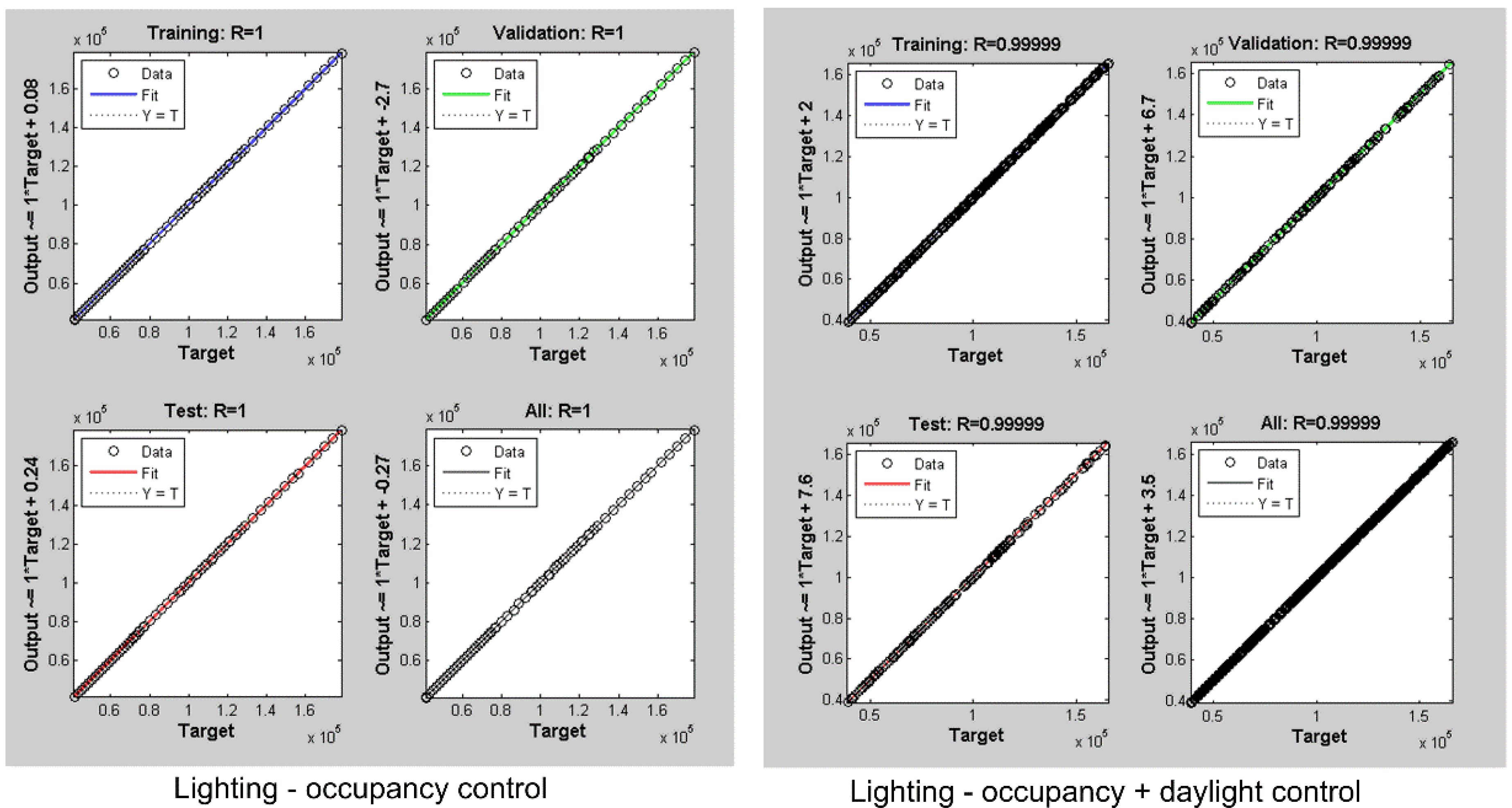
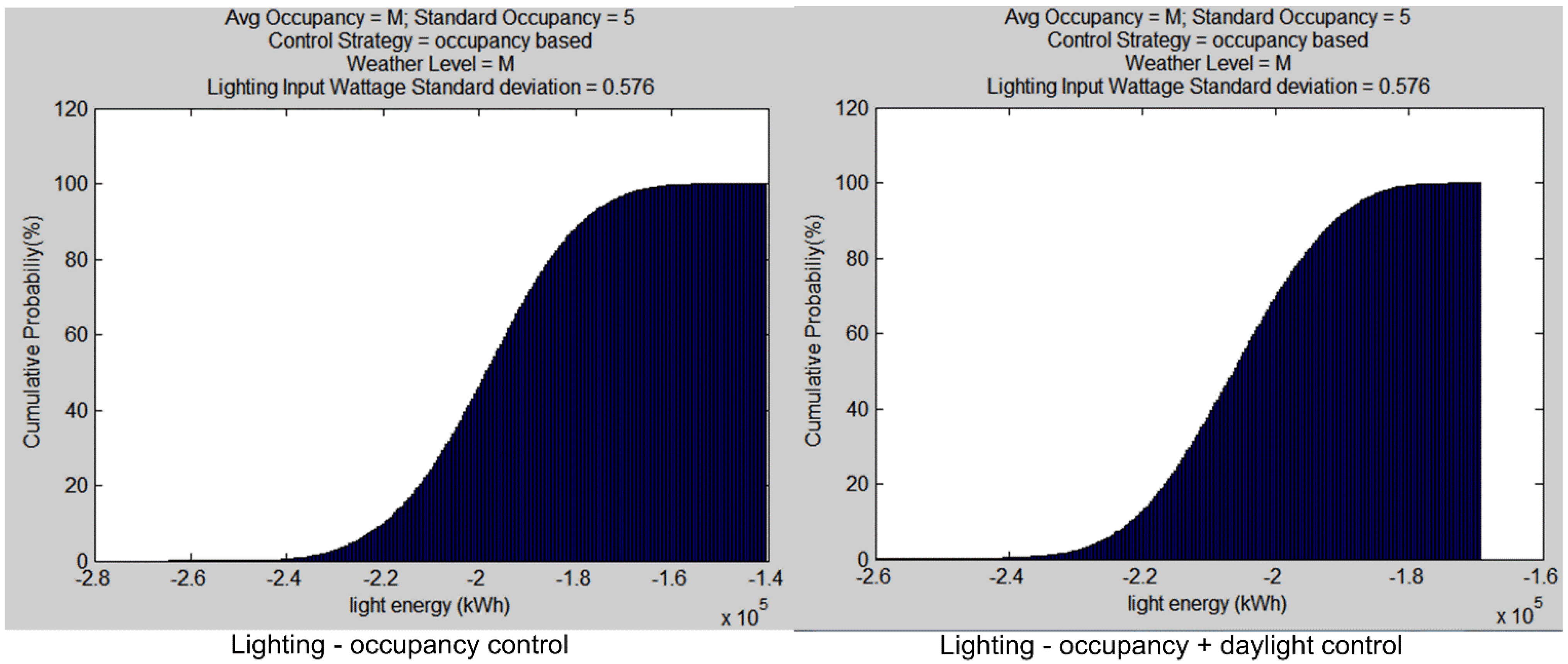
3.4.1. Lighting Energy Consumption

The performance of the neural network model is shown in Figure 8. The target value in Y-axis denotes the simulated value from EnergyPlus. The output value in X-axis denotes the predicted value using surrogate model. The testing and training results indicate that very good performance has been achieved in the model. When the occupancy based control is used, RMSE (root mean square error) is 21.6 kWh, and CV (the coefficient of variation) is less than 0.1%. When the occupancy + daylight control is used, RMSE is 144.3 kWh, and CV is 0.16%. Both of the test results show very good performance with an R value close to one. This result is consistent with the previous study showing that lighting energy consumption has a linear relationship with many building parameters [12].

Figure 8. Neural network training and testing results for lighting energy consumption.

Figure 8. Neural network training and testing results for lighting energy consumption.

To evaluate the risk of reducing lighting power density by replacing an existing luminaire with a retrofit luminaire, one of the requirements is to calculate the distribution of lighting energy savings. In current retrofit decisions, only a fixed value is calculated without knowing the probability, which results in risk. Users can predict the probability distribution of lighting energy savings by setting different scenarios. For example, users can evaluate the risk level when medium sky condition happens in a medium occupied building. In Figure 9, the distribution of the difference between the energy consumption of the two luminaires (A and B) is plotted. The risk scenario is set so that the average occupancy level is about 50% with a standard deviation of 10%, and the weather occurrence is M (medium) level. Different results are shown in the two control strategy types. In the left plot in Figure 9, when the occupancy based control is used, replacing an existing luminaire with a retrofit luminaire with advanced lighting controls results in energy savings ranging from about 240 MWh to 140 MWh. Similarly, in the right plot in Figure 9, the energy savings ranges from 240 MWh to 170 MWh. It is observed that using an occupancy + daylight control has less risk for the lighting retrofit project. The guaranteed minimum energy savings using an occupancy + daylight control (170 MWh) is higher than the minimum savings (140 MWh) using occupancy control. When making retrofit decisions, the cost of adding additional control system should be taken into account.

Figure 9. CDFs of lighting energy difference between retrofit and existing lighting system.

Figure 9. CDFs of lighting energy difference between retrofit and existing lighting system.

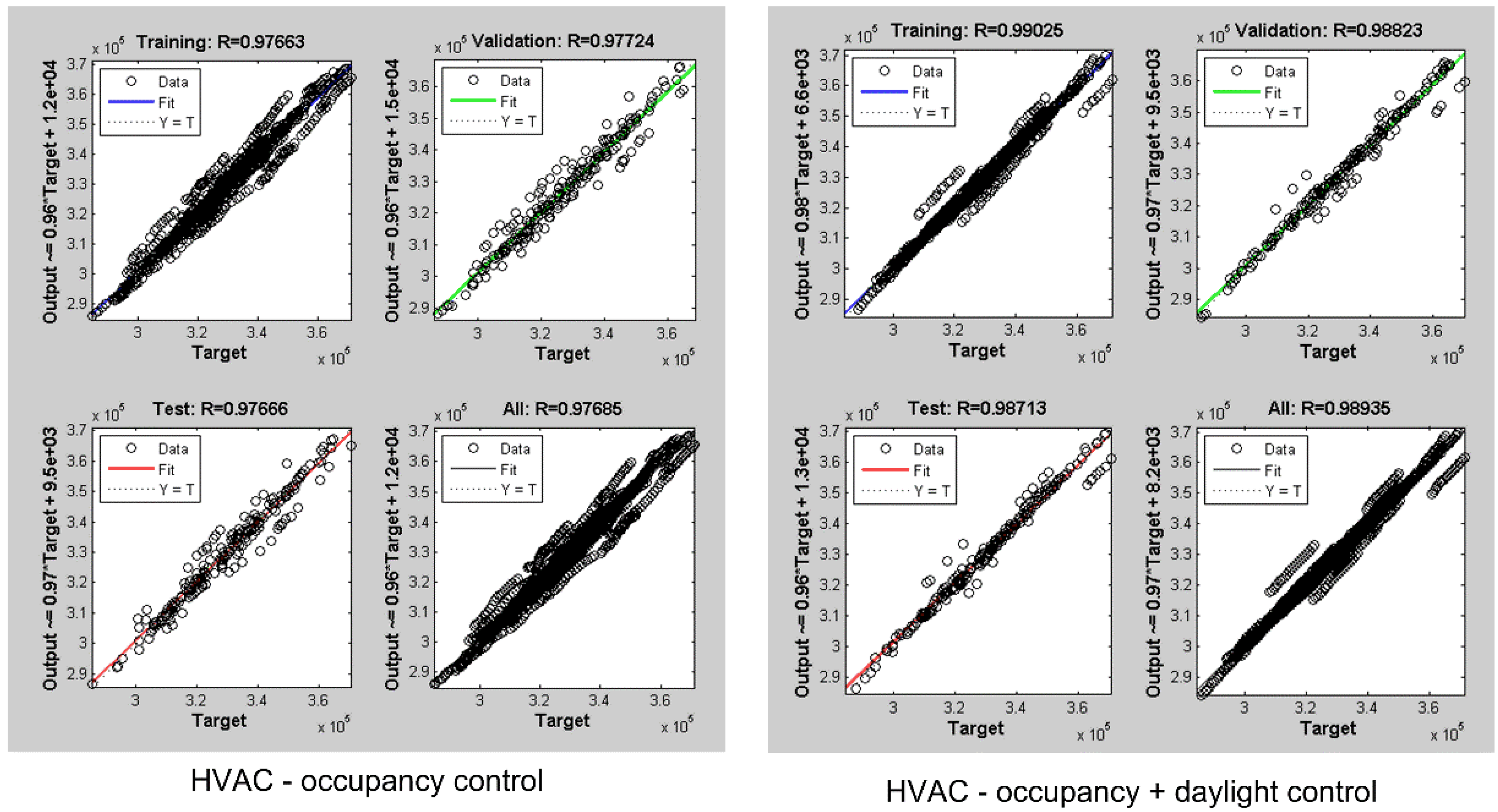
3.4.2. HVAC Energy Consumption

Internal heat emitted from lighting affects HVAC usage, and thus HVAC energy consumption. Neural network model is also used to predict HVAC energy consumption, which has been studied in the literature. In general, the model achieves good performance with R = 0.97–0.98 (see Figure 10). There are a number of factors affecting HVAC energy usage and the prediction accuracy is lower than the accuracy of the lighting energy usage prediction. When the occupancy control strategy is used, RMSE is 1777.5 kWh and CV is 0.54%. When the occupancy + daylight control strategy is used, RMSE is 2693.6 kWh and CV is 0.82%. The error increases when using a complicated lighting control strategy (i.e., occupancy + daylight control).

Figure 10. Neural network training and testing results for HVAC energy consumption.

Figure 10. Neural network training and testing results for HVAC energy consumption.

The probability of the difference between HVAC energy consumption when using the retrofit luminaire with advanced lighting controls and the existing luminaire is plotted (see Figure 11). The occupancy level and weather condition are set to medium. When the occupancy based control is used, the energy consumption increase changed from 15 MWh to 60 MWh. When the occupancy + daylight control is used, the energy consumption increase changed from −100 MWh to 150 MWh, which indicates a larger changing range than the occupancy based control. This is opposite from the case for lighting energy savings. In addition, the CDF curve using occupancy + daylight control (right plot in Figure 11) is smoother than the curve using occupancy control, which indicates a higher standard deviation for HVAC energy savings. The reason that using occupancy + daylight control has a wider range is because the daylight level affects the lighting levels and thus results in fluctuating internal heat gains.

Figure 11. CDFs of HVAC energy difference between retrofit and existing lighting system.

Figure 11. CDFs of HVAC energy difference between retrofit and existing lighting system.

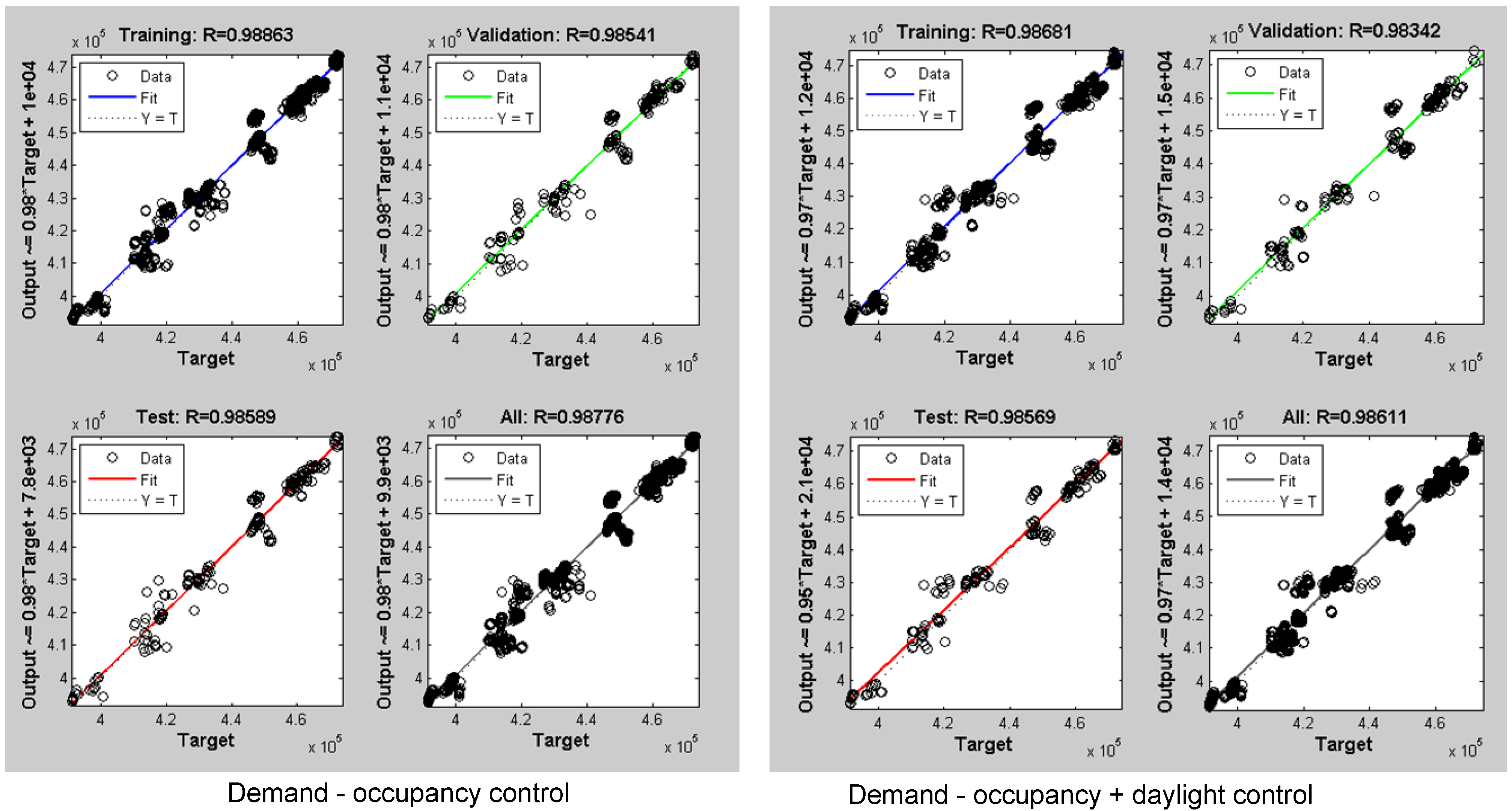
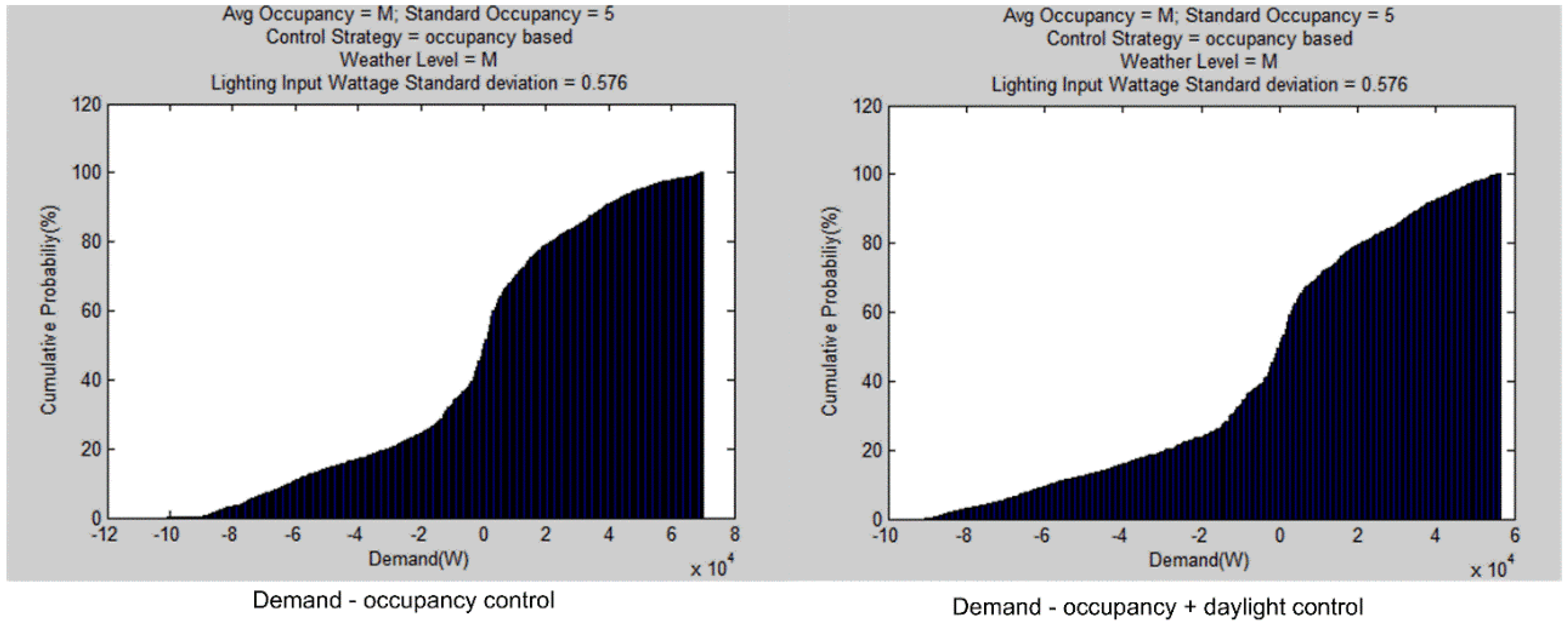
3.4.3. Electricity Demand

An advantage of using the retrofit luminaires with advanced lighting controls is to reduce the electricity peak demand. The electricity demand for the retrofit luminaires with advanced lighting controls is predicted using neural network with good performance (see Figure 12). When the occupancy control is used, RMSE is 3.9 kW and CV is 0.88%. When the occupancy + daylight control is used, RMSE is 7.8 kW and CV is 1.7%. The prediction is reasonably accurate.

Figure 12. Neural network training and testing results for lighting electric demand.

Figure 12. Neural network training and testing results for lighting electric demand.

The difference of the whole building electricity demand using retrofit luminaires with advanced lighting controls and existing luminaires is shown in Figure 13. The two scenarios have a similar pattern. One possible reason is that electricity demand only represents the peak value and thus is less sensitive to luminaire dimming. When the occupancy control is used, the demand difference changes from −100 kW to 70 kW. When the occupancy + daylight control is used, the demand difference changes from −90 kW to 55 kW. The range changes from negative value to positive value, which implies replacing existing luminaires with retrofit luminaires does not always reduce the electricity demand. One possible reason is that HVAC electricity peak value increases while lighting electricity demand decreases. The mean value is expected to reduce the electricity demand.

Figure 13. CDFs of lighting demand difference between retrofit and existing lighting system.

Figure 13. CDFs of lighting demand difference between retrofit and existing lighting system.

3.5. Discussion

In the previous section, the probability distribution plots of lighting and HVAC energy savings and demand difference are presented. Using this information, the mean and standard deviation of these values can be calculated to estimate the risk levels. The expected values and standard deviation of lighting, HVAC, and demand savings are listed in Table 1.

• Lighting Energy Savings: Lighting has the largest energy savings. Both of the two control strategies have small standard deviation, indicating a lower risk.
• HVAC Energy Savings: HVAC energy savings is about 15% of the lighting energy savings. When the occupancy based control is used, the standard deviation is small. However, when the occupancy + daylight control is used, the standard deviation becomes much larger. This is caused by the dimming control of retrofit luminaire with a daylight control system. Thus, the risk level for HVAC energy savings becomes higher when the daylight control is used.
• Electricity Demand: The mean values for both control strategies are similar because the peak value of electricity is less sensitive to the luminaire dimming, and the peak value does not change too much even when using day-lighting control. The standard deviation is much larger. As stated in Section 3.4.3, using the retrofit luminaire with advanced lighting controls may not always reduce the electricity demand because the electricity demand of HVAC may increase. Another reason is that using an existing luminaire may generate more internal heat in winter, and help reduce the HVAC electricity demand. In a whole year, using a retrofit luminaire with advanced lighting controls can still help reduce the electricity demand by about 9 kW on average.

Table 1. Mean and standard deviation of lighting energy savings, HVAC energy savings and demand savings.

Control	Lighting (MWh)		HVAC (MWh)		Demand (kW)
	Occupancy	Occupancy + Daylight	Occupancy	Occupancy + Daylight	Occupancy	Occupancy + Daylight
Mean	201.5	208.0	−30.6	−31.2	9.3	9.4
Standard deviation	16.9	12.3	4.1	39.6	30.8	33.6

Table 1. Mean and standard deviation of lighting energy savings, HVAC energy savings and demand savings.

Control	Lighting (MWh)		HVAC (MWh)		Demand (kW)
	Occupancy	Occupancy + Daylight	Occupancy	Occupancy + Daylight	Occupancy	Occupancy + Daylight
Mean	201.5	208.0	−30.6	−31.2	9.3	9.4
Standard deviation	16.9	12.3	4.1	39.6	30.8	33.6

The probability plots in Section 3.4 are based on the scenario that occupancy and weather control are set to medium. In some buildings or locations, the occupancy levels may change significantly during different months or seasons, or the weather is more variable. Thus the expected value should be calculated from the distribution of the different occupancy levels and weather conditions. The expected value can be calculated using Equation (2). The surrogate model calculates the expected value of the joint distribution.

$$E={\displaystyle \sum _c{\displaystyle \sum _j{P}_c{P}_w\left(S_L(c,w)+S_H(c,w)\right)}}$$

(2)

where E = expected value of energy savings; $P_i^c$ = probability of the occupancy level c; $P_j^w$ = probability of the weather condition w; $S_L(c,w)$ = expected value of the lighting energy savings under occupancy level = c and weather condition = w; and $S_H(c,w)$ = expected value of HVAC energy savings under occupancy level = c and weather condition = w.

Equation (3) shows the runtime ratio between the runtime using the surrogate model and the runtime using a simulation approach. In the equation, the total runtime for the surrogate model based approach includes the training time $T_{train}$ and calculation time $T_{cal}$: (a) In the training time, the training data is generated from simulation. The size of the data samples are generally small; (b) In the calculation time, the surrogate model reads a large number of sampled points to generate a distribution of the energy savings or demand level. Generally, the value of m is much smaller than n (m << n). For example, in the case study, n is more than one million while m is less than one thousand. The total runtime for simulation is easy to compute. In the case study, the surrogate model takes less than one second to calculate the results. However, simulations using EnergyPlus may take more than 1.5 min. The simulation time is significantly reduced.

$$R=\frac{T_{cal}+T_{train}}{t_s\times n}=\frac{t_m\times n+t_s\times m}{t_s\times n}\approx \frac{t_m}{t_s}$$

(3)

where R = Ratio between the runtime using surrogate model and the runtime using simulated based approach; $T_{cal}$ = The total calculation time for surrogate model to generate the probability distribution of the energy savings; $T_{train}$ = The total training time for training the surrogate model using simulated data; $t_m$ = Runtime using surrogate model to generate a single result; $t_s$ = Runtime for a single simulation; $n$ = The number of sampled inputs for surrogate model; $m$ = The number of sampled inputs for training surrogate model.

4. Conclusions

Dynamic simulation can be performed for energy efficient building retrofits in order to predict the effect of retrofit interventions. The large number of simulations done in this process results in long simulation times, and underestimates or overestimates the risk factors because the risk factor space is not correctly sampled. In this research, we developed a method that uses surrogate models as an alternative to current methods that are usually done using physics based simulation tools. The surrogate model uses adaptive sampling to reduce the sample space while maintaining prediction accuracy. The model can predict performance without repeatedly sampling the risk parameters. The probability distributions of the risk factors are evaluated by using Monte Carlo simulation coupled with the surrogate model.

This research targets four main risk factors during a lighting retrofit decision: luminaire input wattage, weather or sky condition, occupancy pattern, and lighting control strategy. Weather distribution data is sampled using historical data and the Sandia method. Occupancy patterns are generated based on a stochastic occupancy model. Two luminaire types (existing luminaire and retrofit luminaire with advanced lighting controls) are evaluated with an input wattage distribution. To test the feasibility and accuracy of this model, a case study was performed using a standard commercial reference office building. The neural network model selected from the surrogate modeling demonstrates good performance. The model can accurately predict lighting and HVAC energy consumption and electricity demand. The probability distribution of retrofit performance is evaluated. The lighting control strategy affects the magnitude of building performance. The lighting energy consumption and HVAC energy consumption show different trends for the two control strategies. The four risk factors affect the distribution function of the building performance and are quantified to provide feedback for decision-makers.

There are some limitations in this research. For example, the surrogate models were validated during the training process. However, the energy savings results (e.g., Figure 9) calculated using surrogate model are not validated and compared with the results using EnergyPlus simulation because it is practically impossible to simulate all the cases (a few million samples) using EnergyPlus. Future work includes adding a ranking function to quantify under which conditions which factor has a higher risk than others, and exploring the financial analysis of the retrofit decision.

References

1. Heo, Y.; Choudhary, R.; Augenbroe, G.A. Calibration of building energy models for retrofit analysis under uncertainty. Energy Build. 2012, 47, 550–560. [Google Scholar] [CrossRef]
2. Asadi, E.; da Silva, M.G.; Antunes, C.H.; Dias, L. Multi-objective optimization for building retrofit strategies: A model and an application. Energy Build. 2012, 44, 81. [Google Scholar] [CrossRef]
3. Murray, S.N.; Walsh, B.P.; Kelliher, D.; O’Sullivan, D.T.J. Multi-variable optimization of thermal energy efficiency retrofitting of buildings using static modelling and genetic algorithms—A case study. Build. Environ. 2014, 75, 98–107. [Google Scholar] [CrossRef]
4. Tian, W. A review of sensitivity analysis methods in building energy analysis. Renew. Sustain. Energy Rev. 2013, 20, 411–419. [Google Scholar] [CrossRef]
5. Lam, J.C.; Wan, K.K.W.; Yang, L. Sensitivity analysis and energy conservation measures implications. Energy Convers. Manag. 2008, 49, 3170–3177. [Google Scholar] [CrossRef]
6. Eisenhower, B.; O’Neill, Z.; Fonoberov, V.A.; Mezić, I. Uncertainty and sensitivity decomposition of building energy models. J. Build. Perform. Simul. 2012, 5, 171–184. [Google Scholar] [CrossRef]
7. Shen, E.; Hu, J.; Patel, M. Comparison of Energy and Visual Comfort Performance of Independent and Integrated Lighting and Daylight Controls Strategies. In ACEEE Summer Study on Energy Efficiency in Industry; American Council for an Energy-Efficient Economy: New York, NY, USA, 2013. [Google Scholar]
8. Shen, E.; Hu, J.; Patel, M. Energy and visual comfort analysis of lighting and daylight control strategies. Build. Environ. 2014, 78, 155–170. [Google Scholar] [CrossRef]
9. Olbina, S.; Hu, J. Daylighting and thermal performance of automated split-controlled blinds. Build. Environ. 2012, 56, 127. [Google Scholar] [CrossRef]
10. Reinhart, C.F.; Herkel, S. The simulation of annual daylight illuminance distributions—A state-of-the-art comparison of six RADIANCE-based methods. Energy Build. 2000, 32, 167–187. [Google Scholar] [CrossRef]
11. Hu, J.; Olbina, S. Radiance-based Model for Optimal Selection of Window Systems. In Proceedings of the ASCE 2012 International Conference on Computing in Civil Engineering, Clearwater Beach, FL, USA, 17 June 2012.
12. Hu, J.; Olbina, S. Simulation-based model for integrated daylighting system design. J. Comput. Civil Eng. 2013, 28. [Google Scholar] [CrossRef]
13. Hu, J.; Olbina, S. Illuminance-based slat angle selection model for automated control of split blinds. Build. Environ. 2011, 46, 786–796. [Google Scholar] [CrossRef]
14. Magnier, L.; Haghighat, F. Multiobjective optimization of building design using TRNSYS simulations, genetic algorithm, and artificial neural network. Build. Environ. 2010, 45, 739–746. [Google Scholar] [CrossRef]
15. Hu, J.; Olbina, S. An Expert System Based on OpenStudio Platform for Evaluation of Daylighting System Design. In Proceedings of the ASCE International Workshop on Computing in Civil Engineering, Los Angeles, CA, USA, 23–25 June 2013; pp. 186–193.
16. Gagne, J.M.L.; Andersen, M.; Norford, L.K. An interactive expert system for daylighting design exploration. Build. Environ. 2011, 46, 2351–2364. [Google Scholar] [CrossRef]
17. Jentsch, M.F.; Bahaj, A.S.; James, P.A. Climate change future proofing of buildings—Generation and assessment of building simulation weather files. Energy Build. 2008, 40, 2148–2168. [Google Scholar] [CrossRef]
18. Yun, G.Y.; Kim, H.; Kim, J.T. Effects of occupancy and lighting use patterns on lighting energy consumption. Energy Build. 2012, 46, 152–158. [Google Scholar] [CrossRef]
19. Forrester, A.I.J.; Keane, A.J. Recent advances in surrogate-based optimization. Prog. Aerosp. Sci. 2009, 45, 50–79. [Google Scholar] [CrossRef]
20. Neto, A.H.; Fiorelli, F.A.S. Comparison between detailed model simulation and artificial neural network for forecasting building energy consumption. Energy Build. 2008, 40, 2169–2176. [Google Scholar] [CrossRef]
21. Wilcox, S.; Marion, W. Users Manual for TMY3 Data Sets; Technical Report NREL/TP-581-43156; National Renewable Energy Laboratory: Golden, CO, USA, 2008. [Google Scholar]
22. Ebrahimpour, A.; Maerefat, M. A method for generation of typical meteorological year. Energy Convers. Manag. 2010, 51, 410–417. [Google Scholar] [CrossRef]
23. SUMO Lab SUrrogate MOdeling (SUMO) Toolbox. Available online: http://www.sumo.intec.ugent.be/SUMO (accessed on 1 August 2013).
24. U.S. Department of Energy Commericial Reference Buildings. Available online: http://energy.gov/eere/buildings/commercial-reference-buildings (accessed on 1 September 2013).
25. American Society of Heating, Refrigerating and Air Conditioning, Inc (ASHREA). Energy Standard for New Buildings except Low-Rise Residential Buildings; ANSI/ASHRAE/IESNA Standard 90.1-1989; ASHREA: Atlanta, GA, USA, 1989. [Google Scholar]