Model-Based Observer Design Considering Unequal Measurement Delays

Abstract

State observers are essential components of a modern control system. It is often designed based on a mathematical model of the process, thus requiring detailed process knowledge. However, in the existing state estimation methods, equal delays are commonly assumed for all communication lines, which is unrealistic and poses problems such as instability and a degraded performance of observers when unequal time delays exist. In this paper, a design of observers considering the measurement delays is presented. To deal with this problem, a chain-based observer has been proposed in which each chain deals with one output delay, performs prediction for the unavailable output value, and passes it to the next chain. Convergence of each chain observer as well as overall state estimation were proven. To illustrate the performance of the proposed scheme, simulation studies were performed on a benchmark continuous stirred tank heater (CSTH) process.

1. Introduction

State observers play a key role in process monitoring, control, and automation by providing estimates of internal state variables using hardware output measurements. Given a process model, observers can be designed by a large number of available methods such as high gain [1], Kalman filter [2], sliding mode [3], and so on. Various types of observers have also been used in the feedback control design in the presence of delays [4,5]. One of the profound challenges in state estimation is that sensor measurements are often time delayed from the actual process outputs. The control problem of dynamic systems with delays has received growing attention in recent years due to novel application areas such as control over networks [6]. This might also occur due to the slow dynamics of physical sensors as well as communication delays from measurements transmitted between different processing units. If these delays are not compensated, they can lead to the performance degradation of the observers and can have a strong impact on their stability and robustness properties [7,8]. When designing an observer or controller for a system affected by such delays, it is often expedient to lump the measurement delay together with any system and actuation delay, as they are indistinguishable in terms of the ideal closed-loop dynamics of the system [9]. However, in some cases, it can be advantageous to model the measurement delays separately from the other delays.

For linear systems, when the system model is available, there exists literature to deal with equal output delays in state estimation [10,11,12]. Assuming equal delays for all output channels is unrealistic due to different communication line lengths or different sensors and technology types. Hence, the involvement of the delay could be in the communication line, be multiple, and different for each channel, which, however, has rarely been studied in the literature. Supposing equal delays will simplify the observer designing step, but can cause similar problems to ignoring them [13]. Others have assumed the delays on outputs [9,14] or states [15], which again, is simpler than considering them in the communication line (out of the process model). Furthermore, an extension of the available model-based methods to data-driven methods is not straightforward (if even it is possible). This paper intends to extend the Luenberger observer design proposed in [16] to account for equal and unequal measurement delays. Then, the subspace-based approach [17] can similarly be extended to design a data-driven observer in the presence of equal and unequal communication delays.

In this paper, we assumed that the output variables were measured but with delays. Furthermore, the delays might be different among the different output variables. Thus, the receiver node needs to be reconstructed to be compatible with the available data. To deal with this problem, a chain observer has been proposed in which each chain collects data, performs prediction, and passes it to the next chain. The chain observer is a common method to deal with delays in nonlinear systems. The idea of achieving the convergence of the state estimate by using a cascade of two observers (elementary chain observer) for a nonlinear system was first proposed in [18], while the idea of using more than two observers in the chain to deal with large measurement delays was proposed in [19]. In [18], it was shown that a chain of two observers is sufficient for asymptotic state reconstruction as long as the measurement delay is below a given threshold, which depends on the Lipschitz constants of the system. When the time delay exceeds such a threshold, more links must be added to the chain [19]. Thus, each observer in the chain is in charge of predicting the system state for a suitable fraction of the total delay. The chain observer method has also been used for dealing with large measurement delays [7].

In the proposed method, the chain observer was used to deal with the multiple un-equal measurement delays. It was proven that the proposed chain observer had the desired stability properties with delay-free measurements, and the design followed a two-step strategy. First, it obtained the delayed state trajectories using delayed measurements with the delay-free observer. These delayed state estimates were then used as predictors that can compensate for the presence of delay. This strategy was shown to converge to true states. In this paper, the convergence of each chain as well as the overall observer was proven. This paper shows the development of the chain observer, which holds stability as well as convergence, along with a new prediction method that is used in each chain.

The main contributions of this paper are as follows:

• Designing an observer by considering equal measurement delays.
• Designing a chain observer to deal with unequal measurement delays.
• Proving the convergence of each chain as well as the overall observer.

The rest of this paper is organized as follows. In Section 2, the preliminaries are presented. The problem formulation is discussed in Section 3. Section 4 presents the theory of the proposed Luenberger-based observer for the case of equal and unequal measurement delays. In Section 5, a simulation through the continuous stirred tank heater (CSTH) process is used to illustrate the performance of the proposed scheme. The paper ends with concluding remarks in the final section.

2. Preliminaries of Model-Based (Luenberger) Observer Design

In this section, we present the preliminaries of designing a model-based observer approach following the work of [17]. Consider a discrete-time LTI (linear time invariant) system, which is described by

$$\begin{array}{l}x\left(k+1\right)=Ax\left(k\right)+Bu\left(k\right)\hfill \\ y\left(k\right)=Cx\left(k\right)+Du\left(k\right)\hfill \end{array}$$

(1)

where u(k) ∈ R^l, y(k) ∈ R^m, and x(k) ∈ Rⁿ represent process input, output, and state variable vectors, respectively. Suppose that the pair (C, A) with A ∈ R^{n × n}, C ∈ R^{m × n} is observable. The s $\left(=n\right)$-order observer with the following state and output equations

z(k + 1) = Gz(k) + Hu(k) + Ly(k) ∈ R^s

(2)

yˆ(k) = Wz(k) + V y(k) + Qu(k) ∈ R^m

(3)

is asymptotically stable, provided that $G$ is stable (all of its eigenvalues lie within the circle one) and the observer parameters $H$, $L$, $Q$, $W$, $V$ satisfy the following Luenberger equations:

T A − GT = LC, H = T B − LD
C = WT + VC, Q = D − VD
G ∈ Rs × s, T ∈ Rs × n, W ∈ Rm × s

(4)

where $z\left(k\right)$ is the observer states related to the process states through the transformation matrix T ∈ R^{s × n} so that $z\left(k\right)=T\widehat{x}\left(k\right)$, where $\widehat{x}\left(k\right)$ is an estimation of true state $x\left(k\right)$.

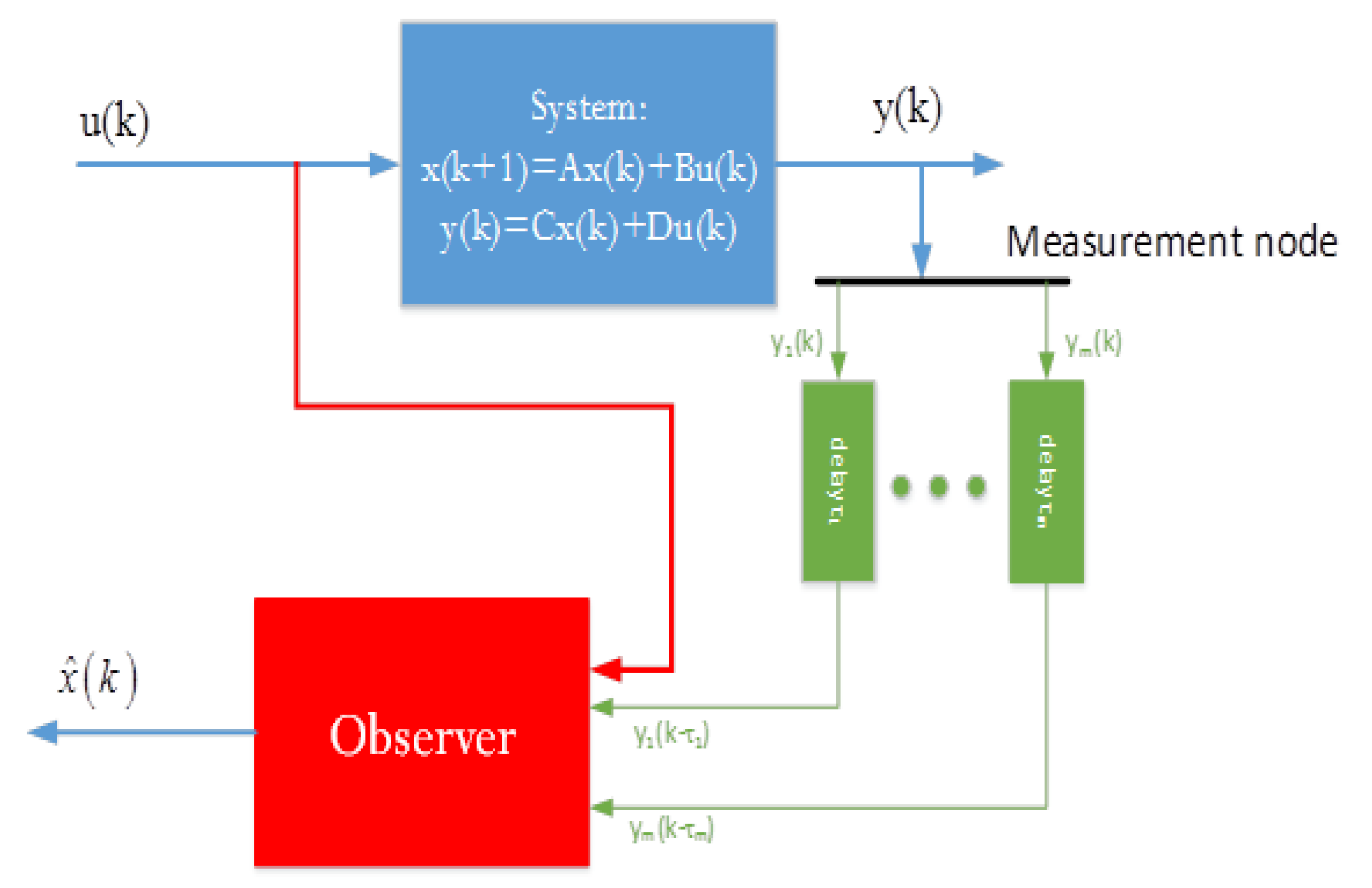
3. Problem Formulation

Sensors and communication networks are an integral part of a data transmission system. One of the main issues regarding measurements and network transmission is the presence of delays in each output measurement (say delay ${\tau }_i$ for output $y_i$). Figure 1 illustrates the communication network and corresponding delays. Due to these delays, output signals $y\left(k\right)$ required for state estimation (2) are not available instantaneously. Therefore, the objective of this work was to design an observer that utilizes delayed measurements (i.e., y(k − τ) = [y₁(k − τ₁) … y_m(k − τ_m)]) to estimate $z\left(k\right)$. As a special case, these delays may be equal in all outputs (i.e., ${\tau }_i=d,$ for $i=1,\dots ,m$.) First, we developed an efficient observer scheme in the presence of constant equal measurement delays. The proposed observer, which deals with equal measurement delays, will have the form of:

$$\begin{array}{l}z\left(k\right)=Gz\left(k-d\right)+{\displaystyle \sum _{i=0}^{d-1}}{H}_{i}u\left(k-1-i\right)+Ly\left(k-d\right)\hfill \\ T\widehat{x}\left(k\right)=z\left(k\right)\hfill \end{array}$$

(5)

where it utilizes available data until the ${\left(k-d\right)}^{th}$ instant to estimate $x\left(k\right)$. The next section will also propose a novel method to deal with unequal measurement delays using a chain–observer structure.

4. The Proposed Observer Design

4.1. Observer Design in the Case of Equal Measurement Delays

In this section, it was assumed that the delays were equal in all outputs (i.e., ${\tau }_i=d$, for $i=1,\dots ,m$). The following theorem designs an asymptotically stable observer (5) with the consideration of equal measurement delays when the system model is available. It is an extension of the Luenberger condition (4) for the case of equal measurement delays.

Theorem 1.

Suppose system model (1) is known with equal measurement delay d in all measured outputs. Furthermore, it is assumed that the pair (C,A) is observable. The observer with the following state and output equations

$$\begin{array}{l}z\left(k\right)=Gz\left(k-d\right)+{\displaystyle \sum _{i=0}^{d-1}}{H}_{i}u\left(k-1-i\right)+Ly\left(k-d\right)\in R^s\hfill \\ T\widehat{x}\left(k\right)=z\left(k\right)\hfill \end{array}$$

(6)

$$\widehat{y}\left(k\right)=Wz\left(k-d\right)+Vy\left(k-d\right)+{\displaystyle \sum }_{i=0}^d{Q}_{i}u\left(k-i\right)$$

(7)

is asymptotically stable, namely$\underset{k\to \infty }{lim}\left(Tx\left(k\right)-z\left(k\right)\right)\to 0$, and has unbiased estimation for$y\left(k\right)$, that is$\underset{k\to \infty }{lim}\left(\widehat{y}\left(k\right)-y\left(k\right)\right)=0$, provided the observer parameters defined in Equations (6) and (7) satisfy the following delayed-Luenberger equations:

State convergence condition:

$$\begin{array}{l}T{A}^d-GT=LC, H_{d-1}=T{A}^{d-1}B-LD,\hfill \\ H_i=T{A}^{i}B, i=0,\dots ,d-2\hfill \end{array}$$

(8)

Output convergence condition:

CA^d = WT + VC, Q₀ = D − VD,
Q_j = CA^j−1B, j = 1,..., d
G ∈ Rs × s, T ∈ Rs × n

(9)

where$G$should be chosen so that it is stable (i.e., every eigenvalue of$G$lies within the circle one). In addition, the closed loop dynamics of estimation error for state and output is reduced to

$$\begin{array}{l}e\left(k\right)=Tx\left(k\right)-z\left(k\right)\hfill \\ e\left(k\right)=Ge\left(k-d\right)\hfill \\ y\left(k\right)-\widehat{y}\left(k\right)=We\left(k-d\right).\hfill \end{array}$$

(10)

 Proof. 

The state equation of Equation (1) can be rewritten as:

$$x\left(k\right)=Ax\left(k-1\right)+Bu\left(k-1\right)$$

(11)

Substituting $x\left(k\right)$ from (11) in (1) yields

$$\left(k+1\right)=A^{2}x\left(k-1\right)+Bu\left(k\right)+ABu\left(k-1\right)$$

(12)

Similarly, $x\left(k-1\right)$ can be replaced by $Ax\left(k-2\right)+Bu\left(k-2\right)$, which yields

$$x\left(k+1\right)=A^{3}x\left(k-2\right)+Bu\left(k\right)+ABu\left(k-1\right)+A^{2}Bu\left(k-2\right)$$

(13)

Continuing the above procedure, after d step reaches

$$\left(k+1\right)=A^{d+1}x\left(k-d\right)+{\displaystyle \sum }_{i=0}^d{A}^{i}Bu\left(k-1-i\right)$$

(14)

or

$$x\left(k\right)=A^{d}x\left(k-d\right)+{\displaystyle \sum }_{i=0}^{d-1}{A}^{i}Bu\left(k-1-i\right)$$

(15)

The state estimation error is defined as

$$\left(k\right)=Tx\left(k\right)-z\left(k\right)$$

(16)

Substituting Equations (15) and (6) in Equation (16) gives

$$\begin{array}{l}e\left(k\right)=T{A}^{d}x\left(k-d\right)+{\displaystyle \sum _{i=0}^{d-1}}T{A}^{i}Bu\left(k-1-i\right)\hfill \\ -Gz\left(k-d\right)-{\displaystyle \sum _{i=0}^{d-1}}{H}_{i}u\left(k-1-i\right)-Ly\left(k-d\right)\hfill \end{array}$$

(17)

Now by substitution of $T{A}^d-GT=LC$, $H_{d-1}=T{A}^{d-1}B-LD$, $H_i=T{A}^{i}B$, and $y\left(k-d\right)=Cx\left(k-d\right)+Du\left(k-d\right)$, the above equation is reduced to

$$\left(k\right)=Ge\left(k-d\right)$$

(18)

The estimation error (18) will converge to zero, provided $G$ is a stable matrix. Performing similar steps for $\widehat{y}\left(k\right)-y\left(k\right)$ gives

$$y\left(k\right)-\widehat{y}\left(k\right)=We\left(k-d\right)$$

(19)

Converging $e\left(k\right)$ to zero proves relation (10). Thus, the proof of Theorem 1 is completed. □

Remark 1.

The matrix G can be defined as follows:

$$G=\left[\begin{array}{cc}{G}_0& g\end{array}\right], g=\left[\begin{array}{c}\begin{array}{c}{g}_1\\ ⋮\end{array}\\ \begin{array}{c}{g}_{s-1}\\ g_s\end{array}\end{array}\right], G_0=\left[\begin{array}{cccc}0& 0& \cdots & 0\\ 1& 0& \cdots & 0\\ ⋮& \ddots & \ddots & \ddots \\ 0& \cdots & 1& 0\\ 0& \cdots & 0& 1\end{array}\right]$$

(20)

then, the designed observer poles are roots of polynomial function x_s−g_sx_s−1−···−g₁ = 0. Therefore, to have the desired performance, one can select proper poles and determine the corresponding polynomial function coefficients (g_i for i = 1,..., s).

4.2. Observer Design in the Case of Unequal Delays

This section considers the extension of the proposed observers (6) and (7) to deal with unequal measurement delay. The proposed observer consists of $m$ chain–observers, each one being in the form of (6) and (7). Without loss of generality, let ${\tau }_1\le {\tau }_2\le \cdots \le {\tau }_m$ and define $d_1={\tau }_1, d_i={\tau }_i-{\tau }_{i-1}, i=2,\dots ,m$. Before explaining the proposed approach of designing the observer considering unequal delay, a theorem that provides stability conditions for a system with multiple delays is presented. This theorem is an extension to the single delay case, which was presented in [20]. The result of this theorem enables us to design an observer with the convergence property.

Theorem 2.

Suppose the system model with the assumption$\Vert A_0\Vert {}_2\ne 0$, is given by

$$x\left(k+1\right)=A_{0}x\left(k\right)+{{\displaystyle \sum }}_{j=1}^N{A}_{j}x\left(k-d_j\right)$$

(21)

where$N$is the value of time delays. Then, it is asymptotically stables if there exists a real symmetric matrix$P > 0$so that:

$$\begin{array}{l}\left(1+{\epsilon }_m\right)A_0^{T}P{A}_0+N\left(\frac{1+{\epsilon }_m}{{\epsilon }_m}\right){\displaystyle \sum _{j=1}^N}{A}_j{}^{T}P{A}_j-P < 0\hfill \\ {\epsilon }_m={\left(N{\displaystyle \sum _{j=1}^N}\Vert A_j\Vert {}_2^2\right)}^{\frac{1}{2}}\Vert A_0\Vert {}_2^{-1}\hfill \end{array}$$

(22)

where$\Vert {\Psi }_2\Vert =\sqrt{{\lambda }_{\max }\left({\Psi }^T\Psi \right)}$

 Proof. 

See Appendix A. □

Remark 2.

When$\Vert A_0\Vert {}_2=0$, system model (21) can be rewritten as

$$\begin{array}{l}x\left(k+1\right)={\displaystyle \sum _{j=1}^N}{A}_{j}x\left(k-d_j\right)\hfill \\ \hspace{0.17em}=A_{1}x\left(k-d_1\right)+{\displaystyle \sum _{j=2}^N}{A}_{j}x\left(k-d_j\right)\hfill \end{array}$$

(23)

Now, define a new variable as$x^{\prime }\left(k\right)=x\left(k-d_1\right)$. Then, the augmented model becomes

$$\begin{array}{l}\left[\begin{array}{c}x\left(k+1\right)\\ \acute{x}\left(k+1\right)\end{array}\right]=\left[\begin{array}{cc}0& 0\\ 0& A_1\end{array}\right]\left[\begin{array}{c}x\left(k\right)\\ \acute{x}\left(k\right)\end{array}\right]+{\displaystyle \sum _{j=2}^N}\left[\begin{array}{cc}{A}_j& 0\\ 0& 0\end{array}\right]\left[\begin{array}{c}x\left(k-d_j\right)\\ \acute{x}\left(k-d_j\right)\end{array}\right]\hfill \\ \hfill \end{array}$$

(24)

or

$$\overline{x}\left(k+1\right)={\overline{A}}_0\overline{x}\left(k\right)+{\displaystyle \sum }_{j=2}^N{\overline{A}}_j\overline{x}\left(k-d_j\right)$$

(25)

where$\overline{x}\left(k\right)=\left[\begin{array}{c}x\left(k\right)\\ \acute{x}\left(k\right)\end{array}\right], {\overline{A}}_0=\left[\begin{array}{cc}0& 0\\ 0& A_1\end{array}\right]$, and ${\overline{A}}_j=\left[\begin{array}{cc}{A}_j& 0\\ 0& 0\end{array}\right]$. Then, Theorem2 can be applied for stability analysis of (25).

Suppose that due to different sensors or measurement techniques or communication topologies, each output measurement is received with a delay that may be different from delays in other output channels. Therefore, in order to estimate the state $x\left(k\right)$ at sample time $k$, the output $y_i$ is only available up to $k-{\tau }_i$ for $i=1,\dots ,m$. The observer gains can be parameterized by the set of the available measurements. In order to handle the unequal measurement delays, we propose constructing a new observer scheme. The proposed observer scheme is shown in Figure 2, in which $y_i\left(1:s\right)$ is the output $i$ from sample $1$ to $s$. The proposed observer gains can be calculated in a composition of $m$ chain–observers, each of which predicts the unavailable output due to measurement delay as well as updates the values of the estimated states and then passes them to the next chain.

The following theorem provides the design of the asymptotically stable chain–observer with the consideration of unequal measurement delays provided that the system model is available.

Theorem 3.

Suppose that A, B, C, D, in Equation (1) are known, andτ = [ τ₁ ^… τ_m] represents unequal measurement delays, and define $d_1={\tau }_1, d_i={\tau }_i-{\tau }_{i-1}, i=2,\dots ,m$. The design of $m$-chain–observer is achieved by solving the chain-Luenberger equations for $i=1,\dots ,m$ chain–observers. The observer $i$ is designed using the estimated output ${\widehat{y}}_{j+1}\left(k-{\tau }_i\right)$ for $j=i,\dots ,m-1$ provided by the previous chain–observers from $1$ to $i-1$ as

$$\begin{array}{l}z\left(k-{\tau }_{i-1}\right)=G_{i}z\left(k-{\tau }_i\right)+L_i\overline{y}\left(k-{\tau }_i\right)\hfill \\ +{\displaystyle \sum }_{i=0}^{d_i-1}{H}_{i}u\left(k-1-i-{\tau }_{i-1}\right)\hfill \end{array}$$

(26)

where

$$\begin{gathered} \widehat{y}\left(k-{\tau }_{i-1}\right)=\left[y_1\left(k-{\tau }_i\right) \cdots y_i\left(k-{\tau }_i\right) {\widehat{y}}_{i+1}\left(k-{\tau }_i\right) {\widehat{y}}_m\left(k-{\tau }_i\right) {\widehat{y}}_m\left(k-{\tau }_i\right)\right] \\ {T}_i\widehat{x}\left(k-{\tau }_{i-1}\right)=z\left(k-{\tau }_{i-1}\right) \end{gathered}$$

and

$$\begin{array}{l}\widehat{y}\left(k-{\tau }_{i-1}\right)=W_{i}z\left(k-{\tau }_i\right)+V_i\overline{y}\left(k-{\tau }_i\right)\hfill \\ +{\displaystyle \sum }_{i=0}^{d_i}{Q}_{i}u\left(k-i-{\tau }_{i-1}\right)\hfill \end{array}$$

(27)

Each chain–observer satisfies the following convergence conditions:

$$T_i{A}^{d_i}-G_j{T}_i=L_{i}C, H_{d_i-1}=T_i{A}^{d_i-1}B-L_{i}D$$

(28)

where$G_i$for$i=1,\dots ,m$should be chosen so that it is stable and should satisfy the stability condition Theorem 2 as

$$\begin{array}{l}\left(1+{\epsilon }_i\right)G_i^{T}P{G}_i+\left(m-i\right)\left(\frac{1+{\epsilon }_i}{{\epsilon }_i}\right){\displaystyle \sum _{j=i+1}^m}{\Phi }_j{}^{T}P{\Phi }_j-P<0\hfill \\ {\epsilon }_i={\left(\left(m-i\right){\displaystyle \sum _{j=i+1}^m}\Vert {\Phi }_j\Vert {}_2^2\right)}^{\frac{1}{2}}\Vert G_i\Vert {}_2^{-1}\hfill \end{array}$$

(29)

where$P>0$, ${\Phi }_j=-L_i{\displaystyle \prod }_{p=i+1}^m{V}_p{W}_j{I}_j$. It follows then, that the constructed observer is asymptotically convergent, and the observer output equation delivers unbiased estimation for$y\left(k\right)$, that is,

$$\underset{k\to \infty }{lim}\left(\widehat{y}\left(k\right)-y\left(k\right)\right)\to 0$$

(30)

 Proof. 

See Appendix B. □

To design an observer with unequal output delay, Theorem 3 can be utilized to construct each chain observer provided that $g_i$ (i.e., $G_i$) in each chain must be selected in such a way that the stability condition (29) is satisfied. Therefore, the chain observer can be designed using the following algorithm (Algorithm 1):

Algorithm 1. Chain observer design algorithm

Step 1: set $i=m$ Step 2: Select a proper $G_i$ that satisfies stability conditions (29). Step 3: Design the chain-observer i using Theorem 1 with $d=d_i$. Step 4: Produce the complementary output $\overline{y}\left(k-{\tau }_{i-1}\right)$ using available output and input, then estimate output data by Equation (27). Step 5: Go to step 2 and repeat till $i=1$.

5. Simulation

In this section, the effectiveness of the proposed approach was demonstrated on a simulation setup of a continuous stirred tank heater (CSTH). The system is written as a linear state-space model to generate input–output data with the following parameters [16]:

$$x=\left[\begin{array}{c}{V}_T\\ H_T\\ T_{hj}\end{array}\right], y=\left[\begin{array}{c}{h}_T\\ T_T\\ T_{hj}\end{array}\right]$$

(31)

$$A=\left[\begin{array}{ccc}0& 0& 0\\ -626.4371& -5.9406\times {10}^{-3}& 36.55\\ 0& 0& -1.2019\times {10}^{-3}\end{array}\right]$$

$$B=\left[\begin{array}{cc}1& 0\\ 0& 0\\ 0& 3041.5241\end{array}\right]$$

(32)

$$C=\left[\begin{array}{ccc}31.831& 0& 0\\ 0& 3.8578\times {10}^{-5}& 0\\ 0& 0& 1\end{array}\right]$$

where ${\dot{V}}_{in}-{\dot{V}}_{out}\equiv u_1, P_h\equiv u_2$ are two input variables, and the water level $h_T$, the temperature of the water in the tank $T_T$ as well as in the heating jacket $T_{hj}$ are output variables. The physical meanings of the process variables and parameters used above are listed in

Table 1. The process variables and parameters.

Symbol	Description	Unit
VT	Water volume in the tank	L
HT	Enthalpy in the tank	J
Thj	Temperature in the heating jacket	°C
${\dot{V}}_{in}, {\dot{V}}_{out}$	Water flows in and out of the tank	1/s
Ph	Electrical heater power	W
hT	Water level in the tank	m
TT	Water temperature in the tank	°C

.

The output variables had the delay vector of τ = [2 5 7]. The order of the observer was s = 3. Set g₁ = [10⁻², −3 × 10⁻⁸, 3 × 10⁻⁴] so that all three poles were located in 10⁻⁴ at each chain. Then, we designed a chain–observer using Algorithm 1 when m = 3.

The following is the design procedure:

Chain 1-

Step $1.1$: Set $d=7-5=2$ and $s=3$;

Step $1.2$: Set

$$g=\left[\begin{array}{c}{10}^{-12}\\ -3\times {10}^{-8}\\ 3\times {10}^{-4}\end{array}\right]$$

(33)

$$G=\left[\begin{array}{ccc}0& 0& {10}^{-12}\\ 1& 0& -3\times {10}^{-8}\\ 0& 1& 3\times {10}^{-4}\end{array}\right]$$

which results in three poles at ${10}^{-4}$.

Step 1.3: Calculate $L$, $T$, $H_i$ as

$$L=\left[\begin{array}{ccc}-3\times {10}^{-7}& -2.3\times {10}^{-6}& 8.3\times {10}^{-12}\\ -1.9\times {10}^{-4}& 6.7\times {10}^{-2}& -5.7\times {10}^{-6}\\ 0.02& 0.0172& -1.2\times {10}^{-6}\end{array}\right]$$

(34)

$$H_1=\left[\begin{array}{cc}1.6\times {10}^{-3}& -2.1\times {10}^{-4}\\ 4.1\times {10}^{-4}& -4.5\times {10}^{-5}\\ -1.3\times {10}^{-4}& 2.4\times {10}^{-5}\end{array}\right]$$

$$T=\left[\begin{array}{ccc}6.2\times {10}^{-3}& -2.6\times {10}^{-6}& 5.7\times {10}^{-6}\\ -0.652& -6.6\times {10}^{-7}& -1.2\times {10}^{-6}\\ -0.732& 2.1\times {10}^{-7}& -6.7\times {10}^{-7}\end{array}\right]$$

$$H_0=\left[\begin{array}{cc}\mathrm{6.21.6}\times {10}^{-3}& 0.175\\ -0.652& 0.038\\ -0.7323& -0.02\end{array}\right]$$

Step $1.4$: Calculate $V$, $W$, $Q_i$ as

$$W=\left[\begin{array}{ccc}-0.32& 1& -0.89\\ 162.21& -507.3& 452.98\\ 246.22& -769.4& 687.04\end{array}\right]$$

(35)

$$V=\left[\begin{array}{ccc}2\times {10}^{-12}& -1.1\times {10}^{-7}& 2.3\times {10}^{-15}\\ 4.5\times {10}^{-6}& 3.5\times {10}^{-5}& 0\\ -1.4\times {10}^{-9}& 8.2\times {10}^{-5}& 1.4\times {10}^{-6}\end{array}\right]$$

$$V=\left[\begin{array}{ccc}2\times {10}^{-12}& -1.1\times {10}^{-7}& 2.3\times {10}^{-15}\\ 4.5\times {10}^{-6}& 3.5\times {10}^{-5}& 0\\ -1.4\times {10}^{-9}& 8.2\times {10}^{-5}& 1.4\times {10}^{-6}\end{array}\right]$$

$$Q_0=\left[\begin{array}{cc}0& 0\\ 0& 0\\ 0& 0\end{array}\right]$$

$$Q_1=\left[\begin{array}{cc}31.83& 0\\ 0& 0\\ 0& 30411.5\end{array}\right]$$

$$Q_2=\left[\begin{array}{cc}0& 0\\ -0.0241& 0\\ 0& -36.55\end{array}\right]$$

Chain 2-

Step $2.1$: Set $d=5-2=3$ and $s=3$;

Step $2.2$: Set

$$g=\left[\begin{array}{c}{10}^{-12}\\ -3\times {10}^{-8}\\ 3\times {10}^{-4}\end{array}\right]$$

(36)

$$G=\left[\begin{array}{ccc}0& 0& {10}^{-12}\\ 1& 0& -3\times {10}^{-8}\\ 0& 1& 3\times {10}^{-4}\end{array}\right]$$

which results in three poles at ${10}^{-4}$.

Step $2.3$: Calculate $L$, $T$, $H_i$

$$L=\left[\begin{array}{ccc}-2.5\times {10}^{-8}& 2\times {10}^{-4}& -1.4\times {10}^{-11}\\ -9.2\times {10}^{-4}& 0.998& 8.27\times {10}^{-11}\\ -1.6\times {10}^{-4}& 0.0236& -1\times 9\end{array}\right]$$

(37)

$$\begin{gathered} H_2=\left[\begin{array}{cc}-1.4\times {10}^{-4}& -3.1\times {10}^{-7}\\ -3\times {10}^{-6}& -4\times {10}^{-7}\\ 6.4\times {10}^{-7}& -3.3\times {10}^{-7}\end{array}\right] \\ T=\left[\begin{array}{ccc}2.9\times {10}^{-2}& -3.8\times {10}^{-5}& -8.2\times {10}^{-11}\\ 5.3\times {10}^{-3}& -9.1\times {10}^{-7}& 1\times {10}^{-9}\\ -4.5\times {10}^{-5}& 8.7\times {10}^{-8}& 1.2\times {10}^{-9}\end{array}\right] \\ {H}_1=\left[\begin{array}{cc}0.0241& -3.2\times {10}^{-8}\\ 5.7\times {10}^{-4}& -3.8\times {10}^{-7}\\ -5.4\times {10}^{-5}& -4.6\times {10}^{-7}\end{array}\right] \\ {H}_0=\left[\begin{array}{cc}0.0295& -2.4\times {10}^{-6}\\ 5.3\times {10}^{-3}& 3\times {10}^{-5}\\ -4.6\times {10}^{-5}& 3.6\times {10}^{-5}\end{array}\right] \end{gathered}$$

Step $2.4$: Calculate $V$, $W$, $Q_i$ as

$$W=\left[\begin{array}{ccc}0.1& -0.53& 6.35\\ 0.007& -0.036& 0.428\\ -1.48& 7.51& -87.86\end{array}\right]$$

(38)

$$\begin{gathered} V=\left[\begin{array}{ccc}-1\times {10}^{-11}& -3\times {10}^{-6}& 2.3\times {10}^{-15}\\ -2.6\times {10}^{-8}& -2.1\times {10}^{-7}& 5\times {10}^{-16}\\ 1.5\times {10}^{-10}& 4.3\times {10}^{-5}& -1.7\times {10}^{-9}\end{array}\right] \\ {Q}_0=\left[\begin{array}{cc}0& 0\\ 0& 0\\ 0& 0\end{array}\right] \\ Q_1=\left[\begin{array}{cc}31.83& 0\\ 0& 0\\ 0& 30411.5\end{array}\right] \\ Q_2=\left[\begin{array}{cc}0& 0\\ -0.0241& 0\\ 0& -36.55\end{array}\right] \\ Q_3=\left[\begin{array}{cc}0& 0\\ 1.4\times {10}^{-4}& 0\\ 0& 0.044\end{array}\right] \end{gathered}$$

Chain 3-Same as Chain 1.

The designed chain–observer (Method 1) was compared with the classic observer (Method 3), which ignores the measurement delays, and the observer (Method 2) [21], which supposes (one) equal measurement delay (delay = 2 in this test). The method proposed in [21] deals with both state and output delays; in this test, state delay is supposed to be equal to zero. Figure 3, Figure 4 and Figure 5 show the estimated values for the system states x₁, x₂, and x₃ by the above-mentioned observers, respectively. These figures show that the proposed observer estimation error converges to zero in 10 s. Observer #2 (considered equal delays) had a bias in estimation and was slow in convergence, and observer #3 (ignored delays) diverged. The input signal to the system is depicted in Figure 6.

Remark 3.

Based on the results presented above, we can conclude that

• By changing the observer poles, the convergence speed can be tuned.
• Each chain is an observer in the form of (6).
• Increasing the communication delays may increase the convergence time and transient estimation error magnitude, but according to theorem 3, it will not make the observer unstable.

6. Conclusions

Delays are an inherent part of any system. Ignoring it could cause instability or degradation in the performances of the control or estimation blocks. Measurement and communication lines produce some delays, which may be unequal due to different line distances or sensor types and technologies. Supposing equal measurement/communication delays causes a similar problem to ignoring them. In this paper, we proposed a new approach to constructing an observer, consisting of a bank of chain–observers to deal with equal and unequal measurement delays. Analytical results for the construction of the observers are provided, and convergence of the chain–observers is shown. Simulations demonstrate the efficacy of the proposed design scheme through a CSTH system in the presence of measurement delays. Having a chain-based observer design facilitates the extension of the proposed approach to a data-driven method. Therefore, the advantage of the proposed approach is that it can be used for designing data-driven (subspace-based) observers [17] in the presence of equal and unequal communication delays. Designing such a data-driven observer is in our future research scope.

References

1. Boizota, N.; Busvelleb, E.; Gauthier, J.-P. An adaptive high-gain observer for nonlinear systems. Automatica 2010, 46, 1483–1488. [Google Scholar] [CrossRef]
2. Youngjoo, K.; Bang, H. Introduction to Kalman filter and its applications. In Introduction and Implementations of the Kalman Filter; Govaers, F., Ed.; IntechOpen: Rijeka, Croatia, 2019. [Google Scholar]
3. Spurgeon, S.K. Sliding mode observers: A survey. Int. J. Syst. Sci. 2008, 39, 751–764. [Google Scholar] [CrossRef]
4. Regaieg, M.A.; Kchaou, M.; Bosche, J.; El-Hajjaji, A.; Chaabane, M. Robust dissipative observer-based control design for discrete-time switched systems with time-varying delay. IET Control Theory Appl. 2019, 13, 3026–3039. [Google Scholar] [CrossRef]
5. Kchaou, M.; Al Ahmadi, S. Robust control for nonlinear uncertain switched descriptor systems with time delay and nonlinear input: A sliding mode approach. Complexity 2017, 2017, 1027909. [Google Scholar] [CrossRef] [Green Version]
6. Karafyllis, I.; Malisoff, M.; Mazenc, F.; Pepe, P. Recent Results on Nonlinear Delay Control Systems; Springer International Publishing: Cham, Switzerland, 2016. [Google Scholar]
7. Nagmani, G.; Karthik, C.; Rajan, G.S. Observer-Based Exponential Stabilization for Time-Delay Systems via Augmented Weighted Integral Inequality. J. Frankl. Inst. 2019, 356, 9023–9042. [Google Scholar] [CrossRef]
8. Gnaneswaran, N.; Joo, Y.H.; Kim, H.S. A linear matrix inequality-based extended dissipativity criteria for linear systems with additive time-varying delays. IFAC J. Syst. Control 2019, 10, 100070. [Google Scholar] [CrossRef]
9. Won, J.K. An Observer for State Estimation in the Presence of Multiple Measurement Delays. Master’s Thesis, California State University, Long Beach, CA, USA, 2019. [Google Scholar]
10. Olbrot, A. Observability and observers for a class of linear systems with delays. IEEE Trans. Autom. Control 1981, 26, 513–517. [Google Scholar] [CrossRef]
11. Zheng, G.; Bejarano, F.J. Observer design for linear singular time-delay systems. Automatica 2017, 80, 1–9. [Google Scholar] [CrossRef]
12. Sanz, R.; Garcia, P.; Krstic, M. Observation and stabilization of LTV systems with time-varying measurement delay. Automatica 2019, 103, 573–579. [Google Scholar] [CrossRef]
13. Cacace, F.; Germani, A.; Manes, C. A chain observer for nonlinear systems with multiple time-varying measurement delays. SIAM J. Control Optim. 2014, 52, 1862–1885. [Google Scholar] [CrossRef]
14. Subbarao, K.; Muralidhar, P.C. A state observer for lti systems with delayed outputs: Time-varying delay. In Proceedings of the 2008 American Control Conference, Seattle, WA, USA, 11–13 June 2008. [Google Scholar]
15. Cao, Y.Y.; Sun, Y.X.; Cheng, C. Delay-dependent robust stabilization of uncertain systems with multiple state delays. IEEE Trans. Autom. Control 1998, 43, 1608–1612. [Google Scholar]
16. Ding, S.X. Data-Driven Design of Fault Diagnosis and Fault-Tolerant Control Systems; Springer: London, UK, 2014. [Google Scholar]
17. Ding, S.X.; Yin, S.; Wang, Y.; Wang, Y.; Yang, Y.; Ni, B. Data-driven design of observers and its applications. In Proceedings of the 18th IFAC World Congress, Milano, Italy, 28 August–2 September 2011. [Google Scholar]
18. Germani, A.; Manes, C.; Pepe, P. State observation of nonlinear systems with delayed output measurements. In Proceedings of the 2nd IFAC Workshop on Time Delay Systems, Ancona, Italy, 11–13 September 2000; pp. 58–63. [Google Scholar]
19. Kahelras, M.; Ahmed-Ali, T.; Giri, F.; Lamnabhi-Lagarrigue, F. Sampled-Data Chain-Observer Design for a Class of Delayed Nonlinear Systems. Int. J. Control 2018, 91, 1076–1090. [Google Scholar] [CrossRef]
20. Stojanovic, S.B.; Debeljkovic, D.L. On the asymptotic stability of linear discrete time delay systems. Eng. Syst. Des. Anal. 2004, 41731, 805–811. [Google Scholar]
21. Dinh Cong, H. A fresh approach to the design of observers for time-delay systems. Trans. Inst. Meas. Control 2018, 40, 477–503. [Google Scholar]
22. Callebaut, D. Generalization of the Cauchy-Schwarz inequality. J. Math. Anal. Appl. 1965, 12, 491–494. [Google Scholar] [CrossRef]
23. Meyer, C.D. Matrix Analysis and Applied Linear Algebra; Siam: Philadelphia, PA, USA, 2000; Volume 71. [Google Scholar]
Figure 1. Schematic showing the transmission lines with measurement delays.
Actuators 10 00281 g001
Figure 2. The proposed m chain–observer (yi (1: s) is the output i from sample 1 to sample s).
Actuators 10 00281 g002
Figure 3. The state 1 estimation results of the three introduced observers.
Actuators 10 00281 g003
Figure 4. The state 2 estimation results of the three introduced observers.
Actuators 10 00281 g004
Figure 5. The state 3 estimation results of the three introduced observers.
Actuators 10 00281 g005
Figure 6. Shows inputs signals of the CSTH system.
Actuators 10 00281 g006