High Precision Motion Control of Electro-Mechanical Launching Platform with Modeling Uncertainties: A New Integrated Error Constraint Asymptotic Design

Abstract

For the demands of a high precision motion control of an uncertain electro-mechanical launching platform, a novel integrated error constraint asymptotic control in the presence of parametric uncertainties and uncertain disturbance is proposed, of which the barrier function method and a continuous asymptotic control design are integrated for the first time. The former technique can effectively avoid excessive tracking errors at the transient phase, which is caused by the disturbance and the large uncertain system parameters’ deviation between the initial estimated value and the actual value, by selecting a proper barrier threshold, while the latter technique can handle the uncertain disturbance to achieve asymptotic tracking. A rigorous stability analysis is given to illustrate the theoretical performance. In addition, as a supplementary measure, repetitive control is employed to estimate and compensate the possible periodic-like disturbance under certain conditions. Two experimental cases on a prototype of a launching platform demonstrate the effectiveness of the proposed controller.

1. Introduction

The launching platform is mainly used to aim at a predetermined target and launch kinetic loads, and has a wide range of applications in military and civilian fields, such as air defense and anti-missile [1], fire suppression and striking the target cumulonimbus in artificial rainfall [2]. Due to the advantages of high response, less pollution and easy layout, electro-mechanical actuation is the most common form of launching platform, and its working principle is shown in Figure 1, which usually includes an actuator load (turret, pylon, etc.), mechanical transmission (coupling, reducer, etc.), drive unit (driver and motor), sensor (resolver, photoelectric encoder, etc.) and controller. The launching platform needs to track the motion commands from the fire control unit as accurately as possible.

The key to achieving high-performance launching lies in designing an excellent motion control strategy. However, the ubiquitous modeling uncertainties (parametric uncertainties and uncertain disturbance) bring great difficulties to the development of the controller, which mainly comes from the poor working conditions [3], such as impact disturbance by the gas jet when launching kinetic loads, the change in the inertial load, the changes in the friction under the launching thermal environment and the time-varying coupling disturbance between each motion axis, and so on. Some traditional linear control methods, such as feedback linearization control [4] and PID combined with feed-forward, are gradually becoming unable to meet the needs of a high precision launching platform, while the model-based nonlinear control has gradually gained recognition and attention. The adaption control can handle the parametric uncertainties well through the online estimation of uncertain parameters and further feed-forward compensation [5,6]. However, it can be easily affected and seems powerless when strong disturbance exists. In fact, the uncertain disturbance, no matter matched or unmatched, has become the main obstacle to improving the motion tracking performance of the electro-mechanical platform. Typical, popular methods to tackle this thorny problem are nonlinear adaptive robust control [7,8], sliding mode control (SMC) [9,10], neural network control [3,11,12], robust integral of the sign of the error (RISE) [13,14], disturbance observer [15,16] and repetitive control [17,18]. All of these methods have been widely used for their core of skillfully coping with the disturbance.

As we all know, asymptotic tracking in which the tracking error gradually converges to zero is the most ideal theoretical result for steady phase and can be beneficial for the launching platform to run for a long time. In the aforementioned existing literature, the RISE controller utilizes a continuous robust integral term to achieve asymptotic control, but the design structure of RISE is slightly complicated and it may accompany the far-fetched assumption that the second derivative of disturbance needs to be bounded [13,14]. Another effective method to realize asymptotic control is SMC [9,10], however the possible jittery control signal may arouse the un-modelled dynamic of the launching platform and weaken the expected performance [19], while, for the novel nonlinear continuous asymptotic control in the presence of uncertain disturbance proposed in [20] for nonlinear systems, it is easy to retrofit the design and convenient to be integrated with other control structures. In addition, for systems with strong parameter uncertainties, the transient tracking performance is also worthy of attention. The authors of [21] propose prescribed performance control, which can improve transient control performance by constraining the overshoot and convergence speed through design functions. However, its design structure is complex, and the controller derivation process is not directly related to the tracking error but a redefined conversion error, which makes it difficult to achieve asymptotic tracking. In addition, the barrier Lyapunov function technology, which makes full use of the characteristic that the Lyapunov function approaches infinity when the control variable approaches to a certain threshold [22] and is mainly used to constrain the state, gives us inspiration that constraining the tracking error through the barrier Lyapunov function may be a good way to further improve the tracking accuracy at the transient phase. However, the disadvantage of the traditional barrier Lyapunov function technology is that uncertain disturbance can easily bring it in to design dilemma.

In this research, we focus on the realistic requirements of improving the global tracking accuracy of electro-mechanical launching platforms with modeling uncertainties. Based on the above analysis and consideration, we try to propose a novel integrated error constraint asymptotic control frame, in which the barrier function method and a continuous asymptotic control design are integrated for the first time. The barrier Lyapunov function is introduced to impose constraint on the tracking error to improve the poor transient position accuracy caused by the disturbance and the large uncertain system parameters deviation between the initial estimated value and the actual value. Furthermore, a nonlinear continuous control law is designed to deal with the remaining uncertain disturbance to achieve asymptotic tracking stability. In addition, as a supplementary measure, repetitive control is employed to estimate and compensate for the possible periodic-like disturbance when the launching platform executes periodic commands.

The remainder of the paper is arranged as follows: system mathematic models are given in the second section, and the third section gives the controller derivation procedure and the main results. Then, the effectiveness of the proposed controller is verified through two experiment cases. The last section comes to the conclusions and future research focus.

2. System Mathematic Models

Schematic diagram of the electro-mechanical launching platform shown in Figure 1, which includes pitch and azimuth subsystems and, for each subsystem, the servo motor is driven by the drivers to rotate the inertial launching load. As in [3,7,14,17,19], the current loop dynamic will be ignored for its response is faster than the mechanical response. We take the azimuth subsystem as the research object, then, considering the coupling disturbance between the two motion axes, the dynamics equation can be described as

$$m\ddot{y}{=k}_{\mathrm{i}}u-F_{\mathrm{f}}\left(\dot{y}\right)-c_1{\omega }_{\mathrm{p}}-c_2{\dot{\omega }}_{\mathrm{p}}-\Delta$$

(1)

where m denotes the inertial load, y, $\dot{y}$, $\ddot{y}$ denote the angle position, angle velocity and angle acceleration of azimuth subsystem, respectively, k_i denotes the voltage-torque gain, F_f($\dot{y}$) denotes the nonlinear friction, ${\omega }_{\mathrm{p}}{,\dot{\omega }}_{\mathrm{p}}$ denote the angle velocity and angle acceleration of pitch axis, respectively, c₁, c₂ denotes the coupling coefficient and Δ denotes the un-modelled dynamic. In this research, the nonlinear friction is modelled as [23]

$$F_{\mathrm{f}}\left(\dot{y}\right){=r}_1\left(\tanh \left(s_1\dot{y}\right)-\tanh \left(s_2\dot{y}\right)\right){+r}_2\tanh \left(s_3\dot{y}\right) {+r}_3\dot{y}$$

(2)

where r₁, r₂, r₃ denotes the weight factors of different friction levels, s₁, s₂, s₃ denotes the shape factors of different friction parts.

Remark 1.

For a physical system, the friction at zero velocity is always non-null because of the static friction and most friction models are discontinuous, as in [24]. However, it is impossible for a motor to produce discontinuous motor force to complete the task [7]. To overcome this technical problem, we chose a continuous model to approximate the actual friction model to facilitate model compensation. In fact, the friction model given in (2) has been widely used in much of the literature [14,25], and it can capture the viscous friction by $r_3\dot{y}$, Coulomb friction by $r_{2}tanh\left(s_3\dot{y}\right)$, Stribeck effect by r₁(tanh(s₁$\dot{y}$ ) − tanh(s₂$\dot{y}$ )) and the stiction coefficient by r₁ + r₂.

Defining the state vectors x = [x₁, x₂]^T = [y,$\dot{y}$]^T, then we can obtain the state space model as

$$\begin{gathered} {\dot{x}}_1{=x}_2 \\ {\theta }_1{\dot{x}}_2=u-{\theta }_2{f}_1\left(x_2\right)-{\theta }_3{f}_2\left(x_2\right)-{\theta }_4{x}_2-{\theta }_5{\omega }_{\mathrm{p}}-{\theta }_6{\dot{\omega }}_{\mathrm{p}}-d \end{gathered}$$

(3)

where θ₁ = m/k_i, θ₂ = r₁/k_i, θ₃ = r₂/k_i, θ₄ = r₃/k_i, θ₅ = c₁/k_i, θ₆ = c₂/k_i, f₁(x₂) = tanh(s₁x₂) − tanh(s₂x₂), f₂(x₂) = tanh(s₃x₂), d = Δ/m denotes the lumped uncertain disturbance.

3. Design of Motion Controller

3.1. Model Transformation

Before designing the final controller, we consider that the launching platform may face the occasion where it needs to execute period commands. On this occasion, all the system states may exhibit periodicity and make the lumped disturbance d appear for a certain periodicity, for that the un-modelled dynamic Δ contains state-related components.

Based on the control idea in [17], we can rewrite (3) as

$$\begin{gathered} {\dot{\mathit{x}}}_1{=\mathit{x}}_2 \\ {\theta }_1{\dot{\mathit{x}}}_2=\mathit{u}-{\theta }_2{f}_1\left({\mathit{x}}_2\right)-{\theta }_3{f}_2\left({\mathit{x}}_2\right)-{\theta }_4{\mathit{x}}_2-{\theta }_5{\omega }_{\mathrm{p}}-{\theta }_6{\dot{\omega }}_{\mathrm{p}}-{\mathit{d}}_{\mathrm{p}}-\tilde{\mathit{d}} \end{gathered}$$

(4)

where d_p and $\tilde{\mathit{d}}$ denote the periodic component and un-periodic component of lumped disturbance, respectively, satisfying

$${\mathit{d}}_{\mathrm{p}}=\mathit{d}-\tilde{\mathit{d}}$$

(5)

Defining the periodic motion command as x_1d with a known period T, i.e., x_1d(t − T) = x_1d(t), then it is easy to analyze and check that

$${\mathit{d}}_{\mathrm{p}}\left(\mathit{t}-\mathrm{T}\right){=\mathit{d}}_{\mathrm{p}}\left(\mathit{t}\right)$$

(6)

By applying Fourier expansion, we can represent d_p as [18]

$${\mathit{d}}_{\mathrm{p}}\left(\mathit{t}\right)=\frac{\mu }{2}+{\displaystyle \sum }_{\mathit{n}=1}^{\mathit{m}}\left({\rho }_{\mathrm{n}}{\sin \mathit{n}\omega \mathit{t}+\lambda }_{\mathit{n}}\cos \mathit{n}\omega \mathit{t}\right) ,\mathit{m}<\infty$$

(7)

where $\omega =2\pi /\mathrm{T}$. To facilitate the subsequent controller derivation, we further define ϑ = [μ, ρ₁, λ₁, …, ρ_m, λ_m]^T denotes the unknown but constant parameter vector and ψ =[1/2, sinωt, cosωt, …, sinmωt, cosmωt]^T. Ultimately, we can transfer model (4) to the following form for final controller derivation:

$$\begin{gathered} {\dot{\mathit{x}}}_1{=\mathit{x}}_2 \\ {\theta }_1{\dot{\mathit{x}}}_2=u-{\theta }_2{\mathit{f}}_1\left({\mathit{x}}_2\right)-{\theta }_3{\mathit{f}}_2\left({\mathit{x}}_2\right)-{\theta }_4{\mathit{x}}_2-{\theta }_5{\omega }_{\mathrm{p}}-{\theta }_6{\dot{\mathrm{\omega }}}_{\mathrm{p}}-{\mathsf{\vartheta }}^{\mathrm{T}}\mathsf{\psi }-\tilde{\mathit{d}} \end{gathered}$$

(8)

Remark 2.

The parameterized definition ϑ^Tψ of periodic disturbance d_p draws on the idea of repetitive control [17,18]. In fact, it is only a supplementary technology to estimate and compensate the periodic components that may exist in the uncertain disturbance. If there are no periodic components in the disturbance for the actual launch platform, the estimation of this item will be zero and repetitive control will not work, which has no effect on the entire proposed control structure.

Assumption: 

(1)

The uncertain parameters satisfy

$$\begin{gathered} \theta \in {\mathsf{\Omega }}_{\theta }{\{\theta \text{:}\theta }_{\min }\le \theta \le {\theta }_{\max }\} \\ \mathsf{\vartheta }\in {\mathsf{\Omega }}_{\mathsf{\vartheta }}\left\{\mathsf{\vartheta }:{\mathsf{\vartheta }}_{\min }\le \mathsf{\vartheta }\le {\mathsf{\vartheta }}_{\max }\right\} \end{gathered}$$

(9)

where θ_min = [θ_1min, θ_2min, θ_3min, θ_4min, θ_5min, θ_6min]^T and θ_max = [θ_1max, θ_2max, θ_3max, θ_4max, θ_5max, θ_6max]^T, ϑ_max and ϑ_min are known constant bounds of ϑ.

(2)

The un-periodic disturbance $\tilde{\mathit{d}}$ satisfies $\left|\tilde{\mathit{d}}(\mathit{t})\right|\le \mathit{\delta }$, where δ denotes unknown constant.

3.2. Final Controller Derivation

Define a set of error quantities as

$${\mathit{z}}_1{=\mathit{x}}_1-{\mathit{x}}_{1\mathit{d}} {,\mathit{z}}_2{=\mathit{x}}_2-{\mathit{\alpha }}_1$$

(10)

where z₁ denotes the motion tracking error, α₁ is the virtual stabilizing function to be designed later.

Then from (10) and (8), we can achieve the expansion of z₂ as

$$\begin{array}{l}{\theta }_1{\dot{\mathit{z}}}_2{=\theta }_1{\dot{\mathit{x}}}_2-{\theta }_1{\dot{\mathrm{\alpha }}}_1\\ =\mathit{u}-{\theta }_1{\dot{\mathit{\alpha }}}_1-{\theta }_2{\mathit{f}}_1\left({\mathit{x}}_2\right)-{\theta }_3{\mathit{f}}_2\left({\mathit{x}}_2\right)-{\theta }_4{\mathit{x}}_2-{\theta }_5{\mathit{\omega }}_{\mathrm{p}}-{\theta }_6{\dot{\omega }}_{\mathrm{p}}-{\mathsf{\vartheta }}^{\mathrm{T}}\mathit{\psi }-\tilde{\mathit{d}}\end{array}$$

(11)

Considering improvement of the transient tracking performance via error constraint, while based on the backstepping design procedure, we first define the following barrier Lyapunov function [22]

$${\mathit{V}}_1=\frac{1}{2}\log \frac{{\mathit{\beta }}_1^2}{{\mathit{\beta }}_1^2-{\mathit{z}}_1^2}$$

(12)

where β₁ denotes the design constant. Obviously, the barrier Lyapunov function has a logarithmic form and handles the property that is V₁ → ∞ as |z₁| → β₁.

Then, taking the time derivative of V₁, we have

$${\dot{\mathit{V}}}_1=\frac{{\mathit{z}}_1{\dot{\mathit{z}}}_1}{{\mathit{\beta }}_1^2-{\mathit{z}}_1^2}=\frac{{\mathit{z}}_1\left({\mathit{x}}_2-{\dot{\mathit{x}}}_{1\mathrm{d}}\right)}{{\mathit{\beta }}_1^2-{\mathit{z}}_1^2}=\frac{{\mathit{z}}_1\left({\mathit{z}}_2{+\mathit{\alpha }}_1-{\dot{\mathit{x}}}_{1\mathrm{d}}\right)}{{\mathit{\beta }}_1^2-{\mathit{z}}_1^2}$$

(13)

From (13), the virtual stabilizing function α₁ can be designed as

$${\mathit{\alpha }}_1{=\dot{\mathit{x}}}_{1\mathrm{d}}-{\mathit{k}}_1\left({\mathit{\beta }}_1^2-{\mathit{z}}_1^2\right){\mathit{z}}_1$$

(14)

Substitute (14) into (13), we arrive at

$${\dot{\mathit{V}}}_1=-{\mathit{k}}_1{\mathit{z}}_1^2+\frac{{\mathit{z}}_1{\mathit{z}}_2}{{\mathit{\beta }}_1^2-{\mathit{z}}_1^2}$$

(15)

For the next design step, defining the Lyapunov function V₂ = V₁ + θ₁z₂²/2 and continuing to take the time derivative of V₂, we have

$$\begin{gathered} {\dot{\mathit{V}}}_2=-{\mathit{k}}_1{\mathit{z}}_1^2+\frac{{\mathit{z}}_1{\mathit{z}}_2}{{\mathit{\beta }}_1^2-{\mathit{z}}_1^2}{+\mathit{z}}_2{\theta }_1{\dot{\mathit{z}}}_2 \\ =-{\mathit{k}}_1{\mathit{z}}_1^2+\frac{{\mathit{z}}_1{\mathit{z}}_2}{{\mathit{\beta }}_1^2-{\mathit{z}}_1^2}{+\mathit{z}}_2\left[\mathit{u}-{\theta }_1{\dot{\mathit{\alpha }}}_1-{\theta }_2{\mathit{f}}_1\left({\mathit{x}}_2\right)-{\theta }_3{\mathit{f}}_2\left({\mathit{x}}_2\right)-{\theta }_4{\mathit{x}}_2-{\theta }_5{\omega }_{\mathrm{p}}-{\mathit{\theta }}_6{\dot{\omega }}_{\mathrm{p}}-{\mathsf{\vartheta }}^{\mathrm{T}}\mathit{\psi }-\tilde{\mathit{d}}\right] \end{gathered}$$

(16)

Thus, from (16), the final controller can be induced as

$$\begin{gathered} {\mathit{u}=\mathit{u}}_{\mathrm{a}1}{+\mathit{u}}_{\mathrm{a}2}{+\mathit{u}}_{\mathrm{s}1}{+\mathit{u}}_{\mathrm{s}2}{+\mathit{u}}_{\mathrm{s}3} \\ {\mathit{u}}_{\mathrm{a}1}{=\hat{\theta }}^{\mathrm{T}}{\mathsf{\phi },\mathit{u}}_{\mathrm{a}2}={\widehat{\mathsf{\vartheta }}}^{\mathrm{T}}{\mathsf{\psi },\mathit{u}}_{\mathrm{s}1}=-{\mathit{k}}_2{\mathit{z}}_2{,\mathit{u}}_{\mathrm{s}2}=-\frac{{\mathit{z}}_1}{{\mathit{\beta }}_1^2-{\mathit{z}}_1^2} \\ \widehat{\theta }={\left[{\widehat{\theta }}_1,{\widehat{\theta }}_2,{\widehat{\theta }}_3,{\widehat{\theta }}_4,{\widehat{\theta }}_5,{\widehat{\theta }}_6\right]}^{\mathrm{T}},\mathsf{\phi }=\left[{\dot{\mathit{\alpha }}}_1{,\mathit{f}}_1\left({\mathit{x}}_2\right){,\mathit{f}}_2\left({\mathit{x}}_2\right){,\mathit{x}}_2{,\mathit{\omega }}_{\mathrm{p}}{,\dot{\mathit{\omega }}}_{\mathrm{p}}\right] \end{gathered}$$

(17)

where $\widehat{\theta },\widehat{\mathsf{\vartheta }}$ denote the parametric estimation, u_a1 denotes the model compensation component, u_a2 denotes the periodic disturbance compensation component, u_s1 denotes the linear robust control component to maintain stability, u_s2 is designed to cancel the cross-term $\frac{{\mathit{z}}_1{\mathit{z}}_2}{{\mathit{\beta }}_1^2-{\mathit{z}}_1^2}$ in (16), k₂ denotes the control gain, u_s3 denotes the asymptotic control component to handle the lumped un-periodic disturbance $\tilde{\mathit{d}}$. $\widehat{\theta },\widehat{\mathsf{\vartheta }}$ and u_s3 will be designed later.

Substituting the final controller (17) into (16), we can obtain

$${\dot{\mathit{V}}}_2=-{\mathit{k}}_1{\mathit{z}}_1^2-{\mathit{k}}_2{\mathit{z}}_2^2{+\mathit{z}}_2{\tilde{\theta }}^{\mathrm{T}}{\mathsf{\phi }+\mathit{z}}_2{\tilde{\mathsf{\vartheta }}}^{\mathrm{T}}\mathsf{\psi }-{\mathit{z}}_2{\tilde{\mathit{d}}+\mathit{z}}_2{\mathit{u}}_{\mathrm{s}3}$$

(18)

where $\tilde{\theta }=\widehat{\theta }-\theta ,\tilde{\mathsf{\vartheta }}=\widehat{\mathsf{\vartheta }}-\mathsf{\vartheta }$ denoting the parametric estimation errors.

Based on (18), we can design the parametric adaptive estimation law $\widehat{\theta },\widehat{\mathsf{\vartheta }}$ and control component u_s3 to achieve the ultimately asymptotic tracking. A feasible design is given by [20]

$$\begin{gathered} \dot{\widehat{\theta }}=-{\mathit{\Gamma }\mathsf{\phi }\mathit{z}}_2,\dot{\widehat{\mathsf{\vartheta }}}=-{\mathit{P}\mathsf{\phi }\mathit{z}}_2 \\ {\mathit{u}}_{\mathrm{s}3}=-\frac{{\mathit{k}}_3{\mathit{z}}_2{\widehat{\delta }}^{\mathrm{2}}}{{\mathit{k}}_3{\mathit{z}}_2\tanh \left[\frac{{\mathit{z}}_2}{\mathit{\eta }\left(\mathit{t}\right)}\right]\widehat{\delta }+\eta \left(\mathit{t}\right)},\dot{\widehat{\delta }}=\mathit{\gamma }\left|{\mathit{z}}_2\right| \end{gathered}$$

(19)

where Γ and P are the adaptive adjustment parameter matrices, $\dot{\widehat{\delta }}$ denotes the estimation of the upper boundary of the lumped un-periodic disturbance, γ is the adjustment parameter, k₃ denotes the control gain, η(t) is a positive function.

Then, to facilitate the stability analysis, we redefine the following final Lyapunov function

$${\mathit{V}=\mathit{V}}_2 + \frac{1}{2}{\tilde{\theta }}^{\mathrm{T}}{\mathit{\Gamma }}^{-1}\tilde{\theta } + \frac{1}{2}{\tilde{\mathsf{\vartheta }}}^{\mathrm{T}}{\mathit{P}}^{-1}\tilde{\mathsf{\vartheta }} + \frac{1}{2\mathit{\gamma }}{\tilde{\delta }}^2$$

(20)

where $\widetilde{\delta }=\widehat{\delta }-\delta$ denotes the estimation error. Taking the time derivative of V, we have

$${\dot{\mathit{V}}=\dot{\mathit{V}}}_2{ + \tilde{\theta }}^{\mathrm{T}}{\mathit{\Gamma }}^{-1}\dot{\widehat{\theta }}+{\tilde{\mathsf{\vartheta }}}^{\mathrm{T}}{\mathit{P}}^{-1}\dot{\widehat{\mathsf{\vartheta }}}+\frac{1}{\mathit{\gamma }}\tilde{\mathrm{\delta }}\dot{\widehat{\delta }}$$

(21)

Substituting (18) and (19) into (21), we continue to have

$$\begin{gathered} \dot{\mathit{V}}\le -{\mathit{k}}_1{\mathit{z}}_1^2-{\mathit{k}}_2{\mathit{z}}_2^2+\left|{\mathit{z}}_2\right|\mathit{\delta }-\frac{{\mathit{k}}_3{\mathit{z}}_2^2{\widehat{\delta }}^2}{{\mathit{k}}_3{\mathit{z}}_2\tanh \left[\frac{{\mathit{z}}_2}{\mathit{\eta }\left(\mathit{t}\right)}\right]\widehat{\delta }+\mathit{\eta }\left(\mathit{t}\right)}+\tilde{\delta }\left|{\mathit{z}}_2\right| \\ =-{\mathit{k}}_1{\mathit{z}}_1^2-{\mathit{k}}_2{\mathit{z}}_2^2+\left|{\mathit{z}}_2\right|\delta -\frac{{\mathit{k}}_3{\mathit{z}}_2^2{\widehat{\delta }}^2}{{\mathit{k}}_3{\mathit{z}}_2\tanh \left[\frac{{\mathit{z}}_2}{\mathit{\eta }\left(\mathit{t}\right)}\right]\widehat{\delta }+\mathit{\eta }\left(\mathit{t}\right)} \\ \le -{\mathit{k}}_1{\mathit{z}}_1^2-{\mathit{k}}_2{\mathit{z}}_2^2+\left|{\mathit{z}}_2\right|\delta -\frac{{\mathit{k}}_3{\mathit{z}}_2^2{\widehat{\delta }}^2}{{\mathit{k}}_3\left|{\mathit{z}}_2\right|\delta ^+\eta \left(\mathit{t}\right)} \\ =-{\mathit{k}}_1{\mathit{z}}_1^2-{\mathit{k}}_2{\mathit{z}}_2^2+\frac{\left|{\mathit{z}}_2\right|\widehat{\delta }\mathit{\eta }\left(\mathit{t}\right)}{{\mathit{k}}_3\left|{\mathit{z}}_2\right|\widehat{\delta }+\mathit{\eta }\left(\mathit{t}\right)} \\ \le -{\mathit{k}}_1{\mathit{z}}_1^2-{\mathit{k}}_2{\mathit{z}}_2^2+\frac{\mathit{\eta }\left(\mathit{t}\right)}{{\mathit{k}}_3} \end{gathered}$$

(22)

From (22), to guarantee the stability analysis, the positive function η(t) should be selected to satisfy the following property

$${{\displaystyle \int }}_0^{\mathit{t}}\mathit{\eta }\left(\mathit{\tau }\right)\mathit{d}\mathit{\tau }\le \mathit{\epsilon }$$

(23)

where ε > 0 denotes a known constant, i.e., the integral of η(t) should be bounded.

Integrating both sides of (22), we finally obtain

$$\mathit{V}\left(\mathit{t}\right)+{{\displaystyle \int }}_0^{\mathit{t}}{(\mathit{k}}_1{\mathit{z}}_1^2{+\mathit{k}}_2{\mathit{z}}_2^2)\mathit{d}\mathit{\tau }\le \mathit{V}\left(0\right)+\frac{\mathit{\epsilon }}{{\mathit{k}}_3}$$

(24)

3.3. Main Results

Provided the initial conditions that |z₁(0)| < β₁, the final controller given in (17) and (19) can guarantee:

(1) All the signals in the close loop system are always bounded, while the tracking error z₁ will always confirmthe error constraint.

(2) Asymptotic motion tracking will be realized, i.e., z₁ → 0 as t → ∞.

Proofs of 1 and 2: see Appendix A.

4. Comparative Experimental Verification

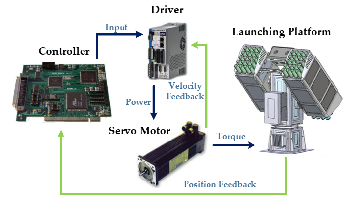
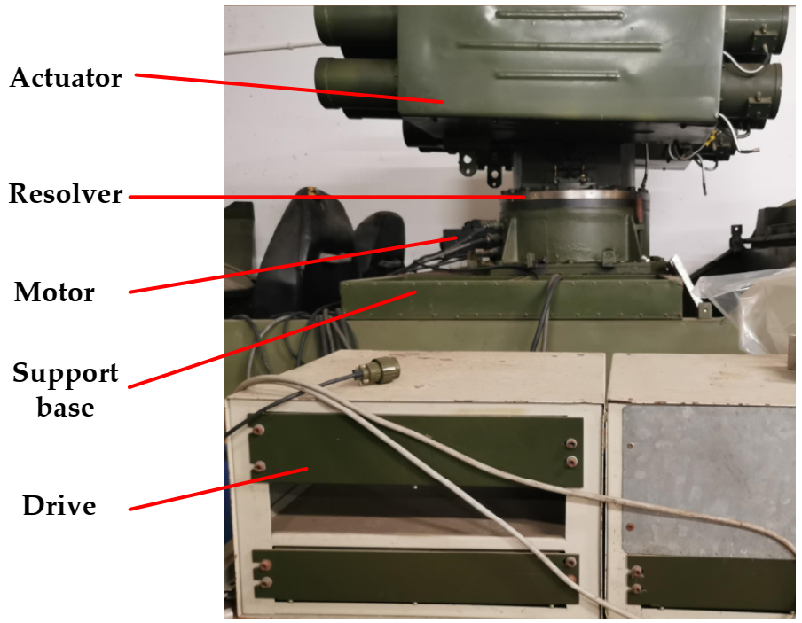
4.1. Experimental Platform

Figure 2 shows the launching platform prototype for the experiment, which is installed on a special vehicle to facilitate field tests. The launching platform includes the pitch and azimuth subsystems, power supply and controller. Each subsystem consists of a Kollmorgen type B-204-A brushless servo motor, a Kollmorgen type AKD-x00307 drive, a reducer, a slewing mechanism and a customized resolver with accuracy ±1′. The controller is designed based on TMS320F28335 DSP. The controller also includes the resolver-digital converter chip AD2S83, which is used to acquire the angular displacement of the launch platform, and the 16-bit digital/analog chip AD5722, which is used to send analog control signals to the drive. The velocity signal is obtained by the backward difference of the high-precision position signal, and the second-order Butterworth filter with a cut-off frequency of 50 HZ is used to attenuate the noise in the velocity signal. The sampling time T is 1 ms.

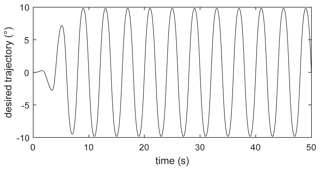
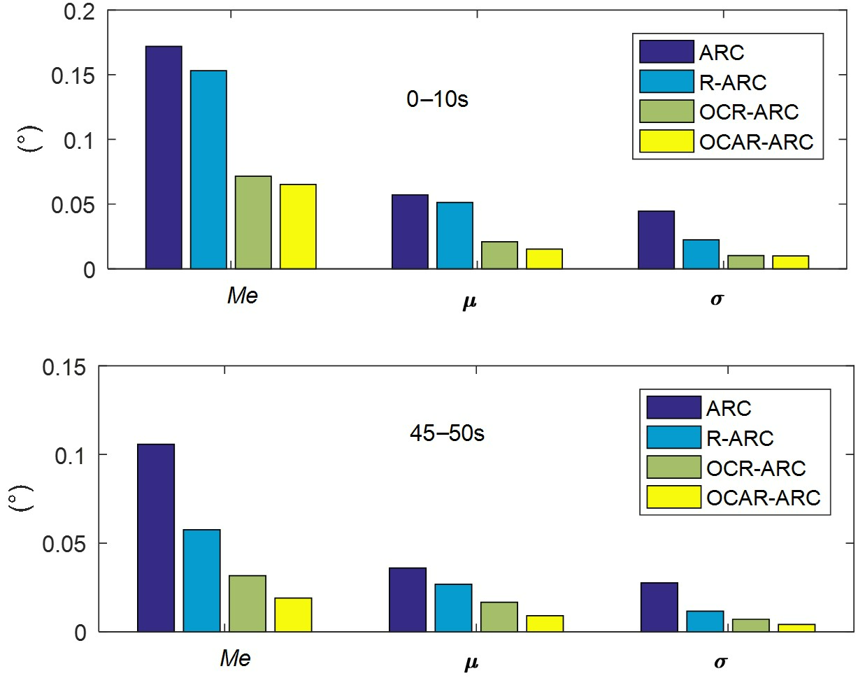
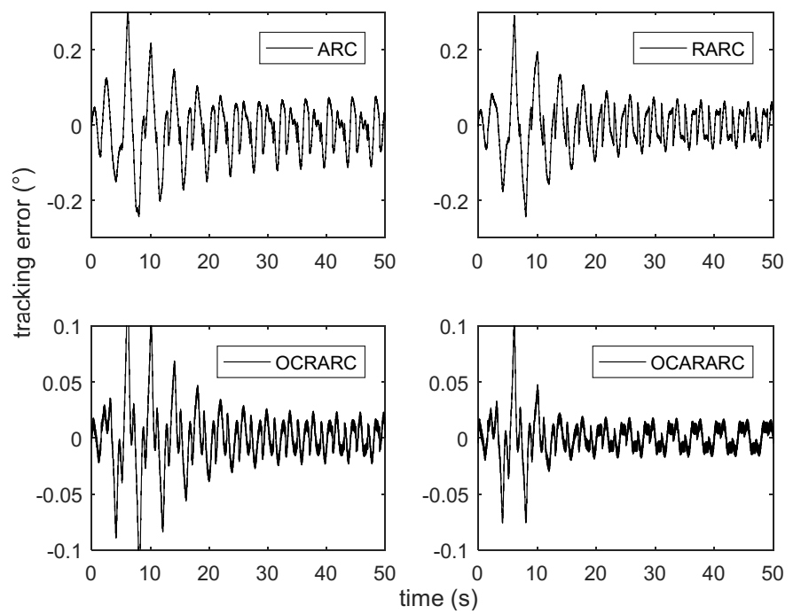
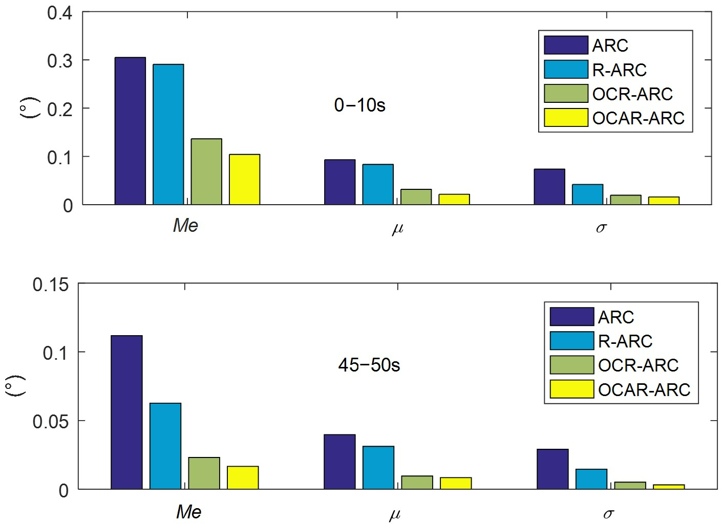
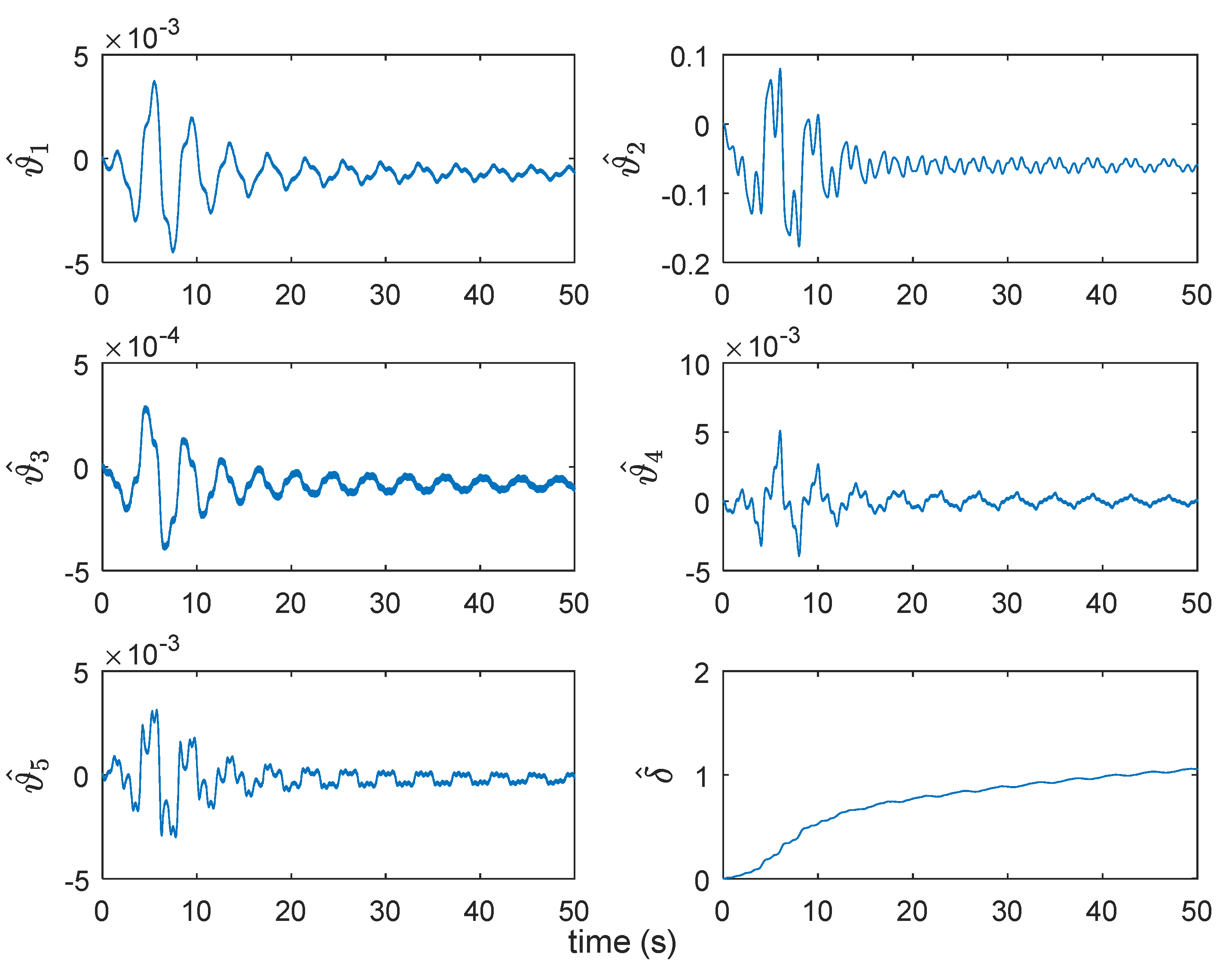
4.2. Comparative Verification Results

In order to fully demonstrate the characteristics and effectiveness of the proposed controller, the following controllers are selected to carry out motion tracking comparative experiments.

(1) OCAR-ARC: This is the controller proposed in this research. The detailed controller structure can be found in (17) and (19). To facilitate the experiment, the number of the Fourier expansion in (7) is taken as m = 2. During the experiment, the initial estimated value of each uncertain system parameter is set so that large parametric errors and tracking errors occur at the initial time, which can help verify the converge performance of the parameter adaptive law and the error constrained ability at the initial stage. The controller parameters are determined by trial and error. Finally, the controller parameters are chosen as: k₁ = 100, k₂ = 10, k₃ = 5, β = 0.5, η(t) =1000/(t² + 0.1) and γ = 20. The initial estimated values of each uncertain parameter are set as θ₀ = [0.001, 0.01, 0.015, 0.1, 0.0015, 0.01]^T, ϑ₀ = [0, 0, 0, 0, 0, 0, 0]^T, and the adaptation matrix Г = diag {0.5, 3, 0.5, 3, 5, 3.5}, P = diag{1 × 10⁻⁵, 50, 5 × 10⁻⁴, 1 × 10⁻⁵, 1 × 10⁻⁵}. In addition, the shape factors of the different friction parts were identified as s₁ = 15 s/rad, s₂ = 1.5 s/rad, s₃ = 700 s/rad during the previous experiment.

Remark 3.

When performing the designed controller, it is not easy to search the optimal parameters to meet the global operating conditions, which requires time-consuming and heavy debugging work and causes it not to be practical. Therefore, we usually use a simple and practical trial and error procedure in experiments. The values determined by this method can approach the locally optimal parameters around the common normal operating conditions. Firstly, we set the barrier thresholdβ as a larger value and set all other parameters as 0. At this time, it can be considered that the barrier function does not impose error constraints. Secondly, we increase control gains k₁ and k₂ until the actuator vibrates significantly or suddenly turns to the limit position, during which the tracking error will be reduced. Then we try to increase the values of matrixΓ, P until the estimation curve of parameters $\widehat{\theta },\widehat{\mathsf{\vartheta }}$reach convergence. Thirdly, we increase control gains k₃, because k₂ and k₃ have a similar function, it is not recommended to increase k₃ too much. Then, we increase the adjusting parameter γ until the estimation curve of  $\widehat{\delta }$reaches convergence and the tracking error decreases significantly. Finally, we start to impose the constraint on the tracking error, that is, we reduce the barrier threshold β to further reduce the tracking error until the actuator vibrates significantly.

(2) ARC: This is the widely used adaptive robust control proposed by Yao et al. in [7]. Based on mathematic model (3), the ARC controller can be synthesized as

$$\begin{gathered} {\mathit{u}=\hat{\theta }}_1{\dot{\mathit{x}}}_{2\mathrm{eq}}{ + \hat{\theta }}_2{\mathit{f}}_1\left({\mathit{x}}_2\right) {+ \hat{\theta }}_3{\mathit{f}}_2({\mathit{x}}_2{) + \hat{\theta }}_4{\mathit{x}}_2{ + \hat{\theta }}_5{\mathrm{\omega }}_{\mathrm{p}}{+\hat{\theta }}_6{\dot{\mathrm{\omega }}}_{\mathrm{p}}-{\mathit{k}}_2{\mathit{z}}_2-\frac{h}{4\mathrm{\epsilon }}{\mathit{z}}_2 \\ {\mathit{z}}_1{=\mathit{x}}_1-{\mathit{x}}_{1\mathit{d}}{,\mathit{z}}_2{=\mathit{z}}_1{+\mathit{k}}_1{\mathit{z}}_1,{\dot{\mathit{x}}}_{2\mathrm{eq}}{=\mathit{x}}_{1\mathit{d}}-{\mathit{k}}_1{\mathit{z}}_1 \\ \dot{\hat{\theta }}{=\mathit{\Gamma }}_{\mathrm{ARC}}{\mathsf{\phi }\mathit{z}}_2,\mathsf{\phi }=\left[{\dot{\mathit{x}}}_{2\mathrm{eq}}{,\mathit{f}}_1\left({\mathit{x}}_2\right){,\mathit{f}}_2\left({\mathit{x}}_2\right){,\mathit{x}}_2\right] \end{gathered}$$

(25)

where h denotes any smooth function satisfying $\mathit{h}\ge \left|\left|{\theta }_{\mathit{m}}\right|\right|{ }^2{\left|\left|\mathsf{\phi }\right|\right|}^2{+\overline{\mathit{d}}}^2{,\theta }_{\mathrm{M}}{=\theta }_{\max }-{\theta }_{\min },\overline{\mathit{d}}$ denotes the upper bound of d, and ε > 0 denotes a design constant. The ARC controller parameters are chosen as: k₁ = 100, k₂ = 10, θ₀ = [0.001, 0.01, 0.015, 0.1, 0.002, 0.002]^T, and Г_ARC = diag{3, 2, 0.5, 1, 10, 1}.

(3) R-ARC: This is the adaptive robust control with periodic disturbance compensation, i.e., u_a2 given in (17) is added to controller ARC. The R-ARC control parameters are chosen as k₁ = 100, k₂ = 10, θ₀ = [0.001, 0.01, 0.015, 0.1, 0.0015, 0.01]^T, ϑ₀ = [0, 0, 0, 0, 0, 0, 0]^T, Г_R-ARC = diag{3, 2, 0.2, 1, 0.5, 3}, P_R-ARC = diag{1 × 10⁻⁴, 100, 1 × 10⁻⁴, 1 × 10⁻⁴, 1 × 10⁻⁴}.

(4) OCR-ARC: In this controller, the barrier function-based tracking error constraint is added to controller R-ARC, that is, this controller is similar to the proposed controller OCAR-ARC but without asymptotic component u_s3. The OCR-ARC control parameters are chosen as k₁ = 100, k₂ = 10, β = 0.5, θ₀ = [0.001, 0.01, 0.015, 0.1, 0.0015, 0.01]^T, ϑ₀ = [0, 0, 0, 0, 0, 0, 0]^T, Г_OCR-ARC = diag{0.1, 2, 0.3,1.2, 0.5, 1.5}, P_OCR-ARC = diag {1 × 10⁻⁶, 30, 1 × 10⁻⁵, 1 × 10⁻⁵, 1 × 10⁻⁶}.

To better measure the motion tracking performance of each controller, three performance indicators related to tracking error are chosen, i.e., the maximum track error M_e, the mean tracking error μ and the mean square error σ. The specific calculation formulas for each indicator are

$$M_{\mathrm{e}}=\underset{i=1,\dots ,\mathit{N}}{\max }\left\{\left|{\mathit{z}}_1\left(\mathit{i}\right)\right|\right\},\mathrm{\mu }=\frac{1}{\mathit{N}}{\displaystyle \sum }_1^{\mathit{N}}\left|{\mathit{z}}_1\left(\mathit{i}\right)\right|,\mathsf{\sigma }=\sqrt{\frac{1}{\mathit{N}}{\displaystyle \sum }_1^{\mathit{N}}{\left(\left|{\mathit{z}}_1\left(\mathit{i}\right)\right|-{\mathrm{\mu }}_{\mathrm{A}}\right)}^2}$$

(26)

where N is the number of the recorded data.

Case 1: Normal motion tracking case

For the actual launch platform, the reference signal is often derived from the random position information generated by the fire control unit related to the enemy target. It can be difficult to give a specific mathematical model for these random position signals, so they are generally not used as reference signals for testing and comparison. In this research, the experimental motion tracking command is set as a functionally processed sinusoidal-like periodic trajectory, i.e., x_1d = 10 atan(sin(0.5πt)[1 − exp(−0.01t³)])° shown in Figure 3. The actual reference signal can be regarded as the superposition of a variety of typical test signals. The running time is 50 s.

Figure 4 shows the tracking errors of the four comparative controllers. Combined with the histogram, Figure 5, of quantitative performance indicators for the initial stage 0–10 s and final stage 45–50 s, it is obvious that OCAR-ARC performs best of the minimum indicators M_e, μ and σ. As mentioned earlier, the proposed controller includes three key technologies, namely barrier function designed in (14) and (17), repetitive control-based periodic disturbance compensation u_a2 designed in (17) and (19), and nonlinear asymptotic control u_s3 designed in (19), whose effectiveness can be verified through pairwise comparison from R-ARC and OCR-ARC, ARC and R-ARC, and OCR-ARC and OCAR-ARC. From the estimation of parameter ϑ in Figure 6, it can be inferred that the periodic disturbance is not zero, so u_a2 has a certain compensation effect, making R-ARC perform better than ARC. The barrier function works globally by constraining the error, so it remarkably improves the tracking performance, especially in the initial stage, which can be easily checked by comparing OCR-ARC and OCAR-ARC with ARC and R-ARC. At the same time, thanks to the asymptotic control u_s3, the tracking error of OCAR-ARC further reduces compared to OCR-ARC. It is worth noting that at the beginning of the system’s operation, tracking errors of the four comparative controllers all fluctuate greatly, which is mainly because the parametric estimations have not yet reached convergence. The estimation of the upper bounds of lumped un-periodic disturbance δ is shown in Figure 6.

Case 2: Input disturbance case

The experimental motion tracking command is set the same as case 1, while the control input is set as u − 0.1x₁ − 0.1x₂, where 0.1x₁, 0.1x₂ denote the position disturbance and velocity disturbance, respectively. The running time is 50 s.

Tracking errors of the four compared controllers are shown in Figure 7. The performance indicators of the initial stage 0~10 s and final stage 45~50 s are shown in Figure 8. The estimations of parameter ϑ and δ are shown in Figure 9. It is obvious that the proposed controllers demonstrate the best performance.

Remark 4.

During the test verification, long-term operation was not carried out. The reason is that, on the one hand, due to the defects in the hardware design of the test launching platform, the system heats up severely after long-term operation. On the other hand, when the launching platform is actually working, in most cases, the position command will be a short-term, real-time command from the fire control unit. From Figure 6 and Figure 9, although in the limited test time, variable$\widehat{\delta }$is continuously increasing, it is clear that the rate of increase is gradually decreasing. Therefore, as the running time increases, variable $\widehat{\delta }$should gradually stabilize. Theoretically, in the steady state, z₁ will be close to zero first, and then z₂ will be close to zero. Variable $\widehat{\delta }$always changes with z₂ and will gradually stabilize, therefore high-gain feedback can be avoided. However, due to the influence of measurement noise and the unmodeled mechanical structure dynamic, the control gain cannot be increased indefinitely, and z₁ and z₂ will gradually converge to a small area, respectively, in the actual working. Even so, high-gain feedback can still be avoided through reasonable parameter tuning.

5. Conclusions

This research proposes a novel high precision motion controller for an electro-mechanical launching platform with modeling uncertainties, which integrates the barrier Lyapunov function method and a nonlinear asymptotic control technology for the first time, while the periodic disturbance compensation is also introduced as a supplement. Combining the theoretical results with two comparative experimental cases carried on launching platform prototype, it can be seen that the proposed controller can significantly improve the tracking accuracy of the initial and final stages, which is of practical value. According to our research plan, the next step will be field performance tests. By cooperating with the fire control unit, the launch platform will need to track random position commands.

References

1. Li, Y.; Yan, Y.; Cai, L. Study of electro-optical measuring system for measuring the swaying of rocket launcher and artillery systems. Def. Technol. 2008, 4, 247–249. [Google Scholar]
2. Hu, J.; Qiu, Y.; Liu, L. High-order sliding-mode observer based output feedback adaptive robust control of a launching platform with backstepping. Int. J. Control 2016, 89, 2029–2039. [Google Scholar] [CrossRef]
3. Hu, J.; Liu, L.; Wang, Y.; Xie, Z. Precision motion control of a small launching platform with disturbance compensation using neural networks. Int. J. Adapt. Control Signal Process. 2017, 31, 971–984. [Google Scholar] [CrossRef]
4. Chiasson, J. A new approach to dynamic feedback linearization control of an induction motor. IEEE Trans. Autom. Control 1998, 43, 391–397. [Google Scholar] [CrossRef]
5. Szabat, K.; Orlowska-Kowalska, T.; Dybkowski, M. Indirect adaptive control of induction motor drive system w an elastic coupling. IEEE Trans. Ind. Electron. 2009, 56, 4038–4042. [Google Scholar] [CrossRef]
6. Underwood, S.; Husain, I. Online parameter estimation and adaptive control of permanent-magnet synchronous machines. IEEE Trans. Ind. Electron. 2010, 57, 4038–4042. [Google Scholar] [CrossRef]
7. Yao, B.; Xu, L. Adaptive robust precision motion control of linear motors with negligible electrical dynamics: Theory and experiments. IEEE-ASME Trans. Mechatron. 2001, 6, 444–452. [Google Scholar]
8. Dong, Z.; Ma, D.; Liu, Q.; Yue, X. Motion control of valve-controlled hydraulic actuators with input saturation and modelling uncertainties. Adv. Mech. Eng. 2018, 10, 1687814018812273. [Google Scholar] [CrossRef]
9. Cheng, X.; Liu, H.; Lu, W. Chattering-suppressed sliding mode control for flexible-joint robot manipulators. Actuators 2021, 10, 288. [Google Scholar] [CrossRef]
10. Wang, P.; Zhu, L.; Zhang, C.; Wang, C.; Xiao, K. Prescribed performance control with sliding-mode dynamic surface for a glue pump motor based on extended state observers. Actuators 2021, 10, 282. [Google Scholar] [CrossRef]
11. Chen, M.; Ge, S.; How, B. Robust adaptive neural network control for a class of uncertain MIMO nonlinear systems with input nonlinearities. IEEE Trans. Neural Netw. 2010, 21, 796–812. [Google Scholar] [CrossRef]
12. Yao, Z.; Yao, J.; Sun, W. Adaptive RISE control of hydraulic systems with multilayer neural-networks. IEEE Trans. Ind. Electron. 2019, 66, 8638–8647. [Google Scholar] [CrossRef]
13. Xian, B.; Dawson, D.M.; de Queiroz, M.S.; Chen, J. A continuous asymptotic tracking control strategy for uncertain nonlinear systems. IEEE Trans. Autom. Control 2004, 49, 1206–1211. [Google Scholar] [CrossRef]
14. Yao, J.; Jiao, Z.; Ma, D. RISE-based precision motion control of DC motors with continuous friction compensation. IEEE Trans. Ind. Electron. 2014, 61, 7067–7075. [Google Scholar] [CrossRef]
15. Wang, Y.; Xiong, Z.; Ding, H. Robust controller based on friction compensation and disturbance observer for a motion platform driven by a linear motor. Proc. Inst. Mech. Eng. Part I-J Syst Control Eng. 2006, 220, 33–39. [Google Scholar] [CrossRef]
16. Deng, W.; Yao, J. Extended-state-observer-based adaptive control of electrohydraulic servomechanisms without velocity measurement. IEEE-ASME Trans. Mechatron. 2020, 25, 1151–1161. [Google Scholar] [CrossRef]
17. Xu, L.; Yao, B. Adaptive robust repetitive control of a class of nonlinear systems in normal form with applications to motion control of linear motors. In Proceedings of the 2001 IEEE/ASME International Conference on Advanced Intelligent Mechatronics, Como, Italy, 8–12 July 2001. [Google Scholar]
18. Yao, J.; Jiao, Z.; Ma, D. A practical nonlinear adaptive control of hydraulic servomechanisms with periodic-like disturbances. IEEE-ASME Trans. Mechatron. 2015, 20, 2752–2760. [Google Scholar] [CrossRef]
19. Dong, Z.; Ma, J.; Yao, J. Barrier function-based asymptotic tracking control of uncertain nonlinear systems with multiple states constraints. IEEE Access 2020, 8, 14917–14927. [Google Scholar] [CrossRef]
20. Zhang, Z.; Xu, S.; Zhang, B. Asymptotic tracking control of uncertain nonlinear systems with unknown actuator nonlinearity. IEEE Trans. Autom. Control 2014, 59, 1336–1341. [Google Scholar] [CrossRef]
21. Bechlioulis, C.; Rovithakis, G. Robust Adaptive Control of Feedback Linearizable MIMO Nonlinear Systems with Prescribed Performance. IEEE Trans. Autom. Control 2008, 53, 1336–1341. [Google Scholar] [CrossRef]
22. Tee, K.; Ge, T. Barrier Lyapunov functions for the control of output-constrained nonlinear systems. Automatica 2009, 45, 918–927. [Google Scholar] [CrossRef]
23. Makkar, C.; Dixon, W.; Sawyer, W.; Hu, G. A new continuously differentiable friction model for control systems design. In Proceedings of the 2005 IEEE/ASME International Conference on Advanced Intelligent Mechatronics, Monterey, CA, USA, 24–28 July 2005. [Google Scholar]
24. Borello, L.; Dalla Vedova, M.D.L. Dry friction discontinuous computational algorithms. Int. J. Eng. Innovative Technol. 2014, 3, 1–8. [Google Scholar]
25. Dong, Z.; Yao, J.; Ma, D. Asymptotic tracking control of motor servo system with input constraint. Acta Armamentarii 2015, 36, 1405–1410. [Google Scholar]
26. Khalil, H. Nonlinear Systems; Prentice-Hall: Upper Saddle River, NJ, USA, 2002. [Google Scholar]
Figure 1. Schematic diagram of electro-mechanical launching platform.
Actuators 10 00331 g001
Figure 2. Launching platform prototype for experiment.
Actuators 10 00331 g002
Figure 3. Desired motion trajectory.
Actuators 10 00331 g003
Figure 4. Global tracking errors of 0–50 s for case 1.
Actuators 10 00331 g004
Figure 5. Tracking performance indicators of 0–10 s and 45–50 s for case 1.
Actuators 10 00331 g005
Figure 6. Estimation of ϑ and δ of the proposed controller for case 1.
Actuators 10 00331 g006
Figure 7. Global tracking errors of 0–50 s for case 2.
Actuators 10 00331 g007
Figure 8. Tracking performance indicators of 0–10 s and 45–50 s for case 2.
Actuators 10 00331 g008
Figure 9. Estimation of ϑ and δ of the proposed controller for case 2.
Actuators 10 00331 g009
Publisher’s Note: MDPI stays neutral with regard to jurisdictional claims in published maps and institutional affiliations.