Use the Force: Review of High-Rate Actuation of Shape Memory Alloys

Abstract

Typical shape memory alloy actuators provide a unique combination of large stresses and strains that result in work-per-volume larger by more than two orders of magnitude than all other actuation methods that are based on active materials. High-rate actuation of shape memory alloys can provide improved energy efficiency, and shorter response and total actuation times, along with large travel-per-wire-length, with respect to slow-rate SMA applications. In this article, we review the different aspects of high-rate actuation of shape memory alloy wires in the high-driving-force regime. We briefly survey previous experimental results about the kinetics and thermodynamics of the phase transformation in view of its practical implications. New experimental results, regarding energy efficiency, total actuation time, repeatability, and fatigue, are presented and discussed. The paper provides general design guidelines for obtaining high actuator performance, as well as guidelines for selecting the source of the electric pulse and its parameters. Finally, we construct and solve detailed simulations of actuator response that can serve as accurate design tools.

1. Introduction

Shape memory alloys (SMA) are smart materials that undergo a phase transformation between two solid phases, martensite and austenite [1]. Heating/cooling of an SMA element beyond the transformation temperature yields large and reversible strains that can be employed in actuator mechanisms.

The martensitic and reverse martensitic phase transformations are diffusionless first-order phase transformations between a high-temperature austenite phase and a low-temperature martensite phase. SMA exhibit strong nonlinear thermo-mechanical behaviors associated with abrupt changes in their lattice structure. The crystallographic symmetry of the austenite is higher than that of the martensite, leading to a variety of symmetry-related degenerate states in the martensite phase called variants [2]. Local domains within the martensite phase that are oriented at different variants are termed twins and the interface between them is termed twin boundary.

When unloaded austenite is cooled below the transition temperature, different parts of the crystal transform to different variants and form a (self accommodated) twinned microstructure, such that the overall macroscopic shape of the crystal remains approximately the same [3]. When subjected to a load at this low temperature, the mixture of variants is converted to variants more favorably oriented with respect to the load (detwinned martensite). For example, under tension, the variant with the longest unit cell parameter lying along the tensile axis will be favorable. The overall process of switching the martensitic variants is called twinning reorientation, and the process of reorienting the martensite phase towards the preferred variant is typically referred to as detwinning [2]. These processes involve an overall significant strain change of several percentages. Since the different variants are energetically equivalent, no driving force exists to return to the mixture of variants upon unloading; thus, the deformation is apparently plastic. Heating above the transformation temperature under little or no load converts it back to the higher symmetry austenite phase, thereby recovering the strains [2]. This process of returning to the original shape is called the shape memory effect. Specific conditioning of the SMA may result in favorable martensitic variants that are oriented in a specific direction, inducing a strain change even at the absence of external loads, typically referred to as the two-way shape memory effect.

SMA-based actuators provide a unique combination of large stresses and strains that result in work-per-volume larger by more than two orders of magnitude than all other actuators that are based on active materials [4]. This advantage has gained SMA actuators significant interest in many medical, automobile, aerospace, wind energy, and industrial applications [5,6,7,8,9,10,11,12,13,14,15,16]. However, conventional SMA actuators suffer from two major drawbacks: slow actuation time and low energy efficiency [10].

The response time of low-driving-force (slow-rate) SMA actuators, in which thermo-mechanical equilibrium is achieved throughout the transformation, is typically restricted by the rate of heat transfer rather than the rate of phase transformation in the SMA element. In fact, SMA wires can be heated very fast using Joule (resistance) heating. This can result in a high driving-force for the transformation allowing for high-rate uni-directional actuation.

Some progress has also been made in the field of active cooling of SMA actuators. It has been shown that various active cooling methods can improve the convective heat transfer coefficient up to eight folds compared with natural convection [17] and five-fold improvement of cyclic actuation [18]. However, the obtainable cooling times remain several orders of magnitudes larger than the heating time scales for single-shot actuation discussed in this paper. Recently, there is a growing interest in such high-rate actuators for single-shot applications, such as release/deployment mechanisms [9,19,20,21,22,23,24], and high-strain-rate mechanical testing of materials [25,26], as well as high-frequency and energy efficient actuation in micro-scale systems [27,28,29,30,31,32].

In studies involving high-rate SMA actuation, heating pulses with duration as short as 1 μs [33,34,35] were generated and tuned by discharging a capacitor onto SMA wires. The resulting mechanical response occurred in the microsecond time scale, dramatically reducing the response time of the actuator. In addition, pulsed heating of SMA wires was shown to be significantly advantageous over slow-rate SMA actuators in terms of energy efficiency and travel-per-length [24,36]. Applications of interest for heat-pulse activation of SMA wires typically require a small number of actuation activations. Repeatability and functional fatigue performances required for such applications are discussed in Section 6.3 and are totally different than fatigue life performances required by slow-rate and low-stress cyclic applications, e.g., as described in Ref. [37].

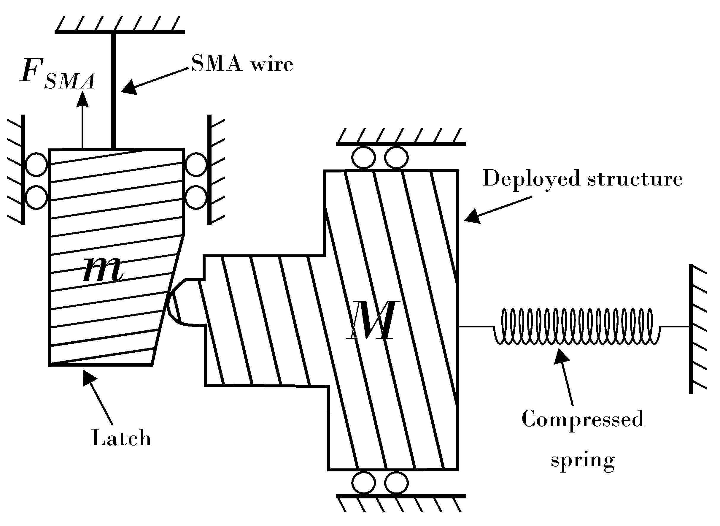
Clever design of mechanical mechanisms activated by the SMA actuator can utilize the fast and powerful actuation capabilities for reducing the required output work and total actuation duration. An example for such application has been demonstrated in Ref. [24], which implemented a release mechanism consisting of a latch that locks/unlocks a deployed device; see Figure 1. The SMA actuator rapidly pulled the latch faster than the motion of the deployed device. As a result, the contact between the latch and the deployed device was disconnected, and the friction forces between them decreased to approximately zero, effectively decreasing the required work. This mechanical design concept, combined with the improved energy efficiency that characterizes high-rate SMA actuators, reduced the required input energy by an order of magnitude compared to a slower-rate SMA-based release mechanism [24].

Table 1. Comparison of a selection of previous studies of the thermo-mechanical response of SMA wires under electric pulse heating with respect to heat pulse duration, power source and boundary conditions.

Reference	Actuator Scale	Mechanical Boundary Conditions	Characteristic Times				Source of Electric Pulse	Voltage Range
			Heat Pulse Duration (${\mathit{\tau }}_{\mathit{e}}$)	Phase Transformation Kinetics ($\mathit{\tau }$)	Mechanical Response Time ${}^1$ $\left(\frac{\mathit{\pi }}{2{\mathit{\omega }}_{\mathit{eff}}}\right)$	Actuation Time ${}^2$ (${\mathit{t}}_{\mathit{actuation}}$)
Volkov et al. (2018) [35]	mm	Free. No loads.	∼1 μs	∼1 μs	Irrelevant ${}^3$	Irrelevant	Discharged capacitor	∼1 kV
Vollach et al. (2017) [38,39]	mm	Clamped at both ends	∼1 μs	∼28 μs	Irrelevant	Irrelevant	Discharged capacitor	2–4 kV
Dana et al. (2021) [34]	mm	Clamped at both ends	∼1 μs	∼30 μs	Irrelevant	Irrelevant	Discharged capacitor	2–4 kV
Vollach et al. (2016) [33]	mm	Hanged mass	∼1 μs	∼28 μs	1–5 ms	1–5 ms	Discharged capacitor	2–4 kV
Malka and Shilo (2017) [24]	mm	Hanged mass and friction force	80–300 μs	Dominated by heating rate	∼200 μs	∼500 μs	Discharged capacitor	200–330 V
Motzki et al. (2018) [36]	mm	Movable mass and spring	1.5–40 ms	Dominated by heating rate	∼20 ms	20–50 ms	DC power supply	24–125 V
Barnes et al. (2006) [19]	mm	Hanged mass and friction force	3–5 ms	Dominated by heating rate	∼0.36 ms	3–5 ms	Discharged capacitor	90 V
Otten et al. (2013) [9]	mm	Movable mass and spring and friction force	6 ms	Dominated by heating rate	∼2 ms	6 ms	Discharged capacitor	50 V
Redmond et al. (2010) [21]	mm	Movable mass and spring and friction force	20–50 ms	Dominated by heating rate	∼6 ms	20–50 ms	DC power supply	40 V
Knick et al. (2019) [30]	m	Movable mass and spring	0.3 ms	Dominated by heating rate	∼25 μs	∼0.33 ms	DC power supply	0.5 V

${}^1$ Characteristic time at which the mechanical system responds; considered as a quarter of the time period of the natural frequency (see Section 6.2). ${}^2$ The time at which the stress in the wire returns to its initial value. ${}^3$ The term ‘irrelevant’ refers to the inability to calculate the natural frequency of the system due to the lack of a moving mass element.

reviews previous studies of the thermo-mechanical response of SMA wires under electric pulse heating. The mechanical boundary conditions (third column) to which the SMA wire is subjected indicate the purpose of the study and potential related applications (as demonstrated in the following paragraphs).

Volkov et al. [35] studied SMA wires that were completely free of mechanical loads and constrains. In this configuration, the wire does not act as an actuator, but the experimental results enable studying the response of the phase transformation, an open and interesting topic in materials science. They found that the phase transformation begins within ∼1 μs after the wire temperature reaches the transformation temperature.

Vollach et al. (2017) [38,39] studied the kinetics and thermodynamics of the phase transformation under conditions at which the response is restricted neither by heat transfer nor by mechanical inertia. To apply these conditions, they clamped the wire at both ends. In this configuration, the wire does not perform external work because there are no moving parts, but the mechanical constrains result in a significant internal stress. This configuration is relevant for applications in which the actuator is required to break a safety pin.

Dana et al. [34] studied the kinetics of the reverse martensitic transformation by using time-resolved X-ray diffraction at synchrotron radiation to measure the in-situ microscopic phase content in a thin layer near the wire surface. Their mechanical boundary conditions were similar to those in Refs. [38,39]. The simultaneous measurement of the microscopic phase content and macroscopic stress provided evidence on the spatial evolution of transformation in high-quality polycrystalline NiTi wires. In particular, they found that the microscopic response occurred within approximately 5 μs of the heating pulse on the wire surface and that the bulk of the wire followed suit after approximately 20 μs. These results provide insight to the mechanisms by which the phase transformation propagates (e.g., by the evolution of macroscopic phase fronts).

References [9,21,24,33,35,36] applied mechanical conditions that are relevant for actuators, clamping the SMA wire at one end, while the other drives a mechanical part or an object (e.g., a hanging mass), generating work. The hanged mass may be allowed to move freely [33,40], subjected to a friction force due to contact with a deployed mechanical part [19,24], or connected to a spring [36]. Refs. [9,21] studied a combination of a spring and friction.

The paper is organized as follows. In Section 2, we provide general design guidelines for obtaining high energy efficiency, short actuation times, and large travel-per-wire-length. In Section 3, we present guidelines for selecting the source of the electric pulse and its parameters (see the two right columns in Table 1). In Section 4, we present typical experimental results and their main features, discussing differences and similarities between the clamp-free and the clamp-clamp configuration. In Section 5, we briefly survey previous results about the kinetics and thermodynamics of the phase transformation in view of its practical implications. In Section 6, we present new experimental results regarding energy efficiency, total actuation time, and discuss repeatability and fatigue. In Section 7 and Section 8, we construct and solve detailed simulations of actuator response that can serve as accurate design tools. Section 7 and Section 8 focus on the clamp-free actuator configuration, in which the actuated mass can move freely, but show how the developed simulations can be expanded to consider cases in which the motion of the mass is subjected to external forces, such as friction or a restoring spring. Finally, in Section 9, we conduct a discussion of the different aspects of SMA actuation considered above, and in Section 10, we summarize and present our main conclusions.

2. Thermo-Mechanical Design Guidelines

2.1. Force and Work Outputs

The work output per unit volume produced by a clamp-free SMA wire undergoing a phase transformation is given by

$$U_{out}=-\underset{{\epsilon }_0}{\overset{{\epsilon }_{el}^A}{\int }}\sigma \mathrm{d}\epsilon ,$$

(1)

where $\sigma$ is the stress in the SMA wire, ${\epsilon }_0$ is the initial pre-elongation (detwinning) strain of the martensite, and ${\epsilon }_{el}^A$ is the final elastic strain at the austenite phase, which is much smaller than ${\epsilon }_0$. For a given sample, the value of ${\epsilon }_0$ is typically determined by the manufacturing process of the NiTi wire, thermo-mechanical treatments it was subjected to, and the applied stress prior to actuation. The value of ${\epsilon }_0$ is usually bounded in the range of 3–6%, which for a given sample under given conditions may be considered as an approximately fixed property. Therefore, the evolved stress during the phase transformation is the main factor that determines the work output (see, e.g., illustrations in Figure 2). Stress is roughly related to the temperature of the wire. At temperatures below the austenite start temperature, $A_s$, there is no phase transformation, no strain change, and $U_{out}=0$. For temperatures T above $A_s$, the relation between the equilibrium stress ${\sigma }_{eq}$ and the temperature is given by the specialized Clausius-Clapeyron equation [39]

$$\frac{\mathrm{d}{\sigma }_{eq}}{\mathrm{d}T}=\frac{H}{T{\epsilon }_0},$$

(2)

where H is the latent heat. Thus, to obtain high stress levels and work output, the temperature T should be much higher than $A_s$ (cf. Section 5 for a detailed discussion of Equation (2)). In a certain range of temperature values obeying ${(T-A_s)}^2\ll A_s^2$, this relation is approximately linear. An upper bound for T typically exists due to various failure mechanisms to which the wire may be subjected (e.g., melting, fatigue, or shape-setting processes).

2.2. Input Electric Energy

The input electric energy per unit volume of the NiTi wires is given by

$$U_{in}\left(t\right)=\rho C_p[T\left(t\right)-T_R]+Hx\left(t\right)+Q\left(t\right),$$

(3)

where $\rho$ and $C_p$ are, respectively, the density and heat capacity of NiTi, $T\left(t\right)$ is the temperature of the wire, and $T\left(0\right)=T_R$ is the room temperature. The second term represents the effect of the latent heat H of the phase transformation, where $x\left(t\right)$ is the volume fraction of austenite. The last term, $Q\left(t\right)$, is the wasted heat that is dissipated from the wire to its surrounding. The characteristic time of $Q\left(t\right)$ is on the order of 1 s, i.e., larger by several orders of magnitude than the heat-pulse duration; therefore, this term is negligible in rapid heating applications. Note that $\rho$ and $C_p$ of the martensite and austenite phases are approximately the same [41]; therefore, H is approximately constant as a function of temperature.

The input energy $\rho C_p(A_s-T_R)$, required for heating the wire up to $A_s$ does not provide any work output. Assuming that, at the end of the actuation stroke, the phase transformation is complete, i.e., $x=1$, the second term in the right-hand side of Equation (3) results in the additional uptake of the constant energy H. Under a slow heating rate, the phase transformation starts as soon as T is just slightly above $A_s$. Then, most of the additional supplied energy goes to the latent and wasted heat, and the SMA temperature remains just slightly above $A_s$. As a result, the evolved stress in the SMA wire is small (see Equation (2)), and the work output is small (Equation (1)), while the input energy is large, leading to a poor energy efficiency.

2.3. High-Rate SMA Actuators

Inducing a martensite-to-austenite transformation in an SMA wire at a temperature much above $A_s$, is a difficult task. One way to achieve this goal is by heating faster than the phase transformation rate, i.e., forming conditions in which ${\dot{U}}_{in}\gg H\dot{x}$ (see Equation (3)), where the dot operator is the time derivative. This approach has been explored to the extreme by Vollach et al. [33], who generated electric pulses with a characteristic time of approximately ${\tau }_e\approx 1$ μs (cf. Table 1). They studied the kinetics of the phase transformation and found two characteristic times of $x\left(t\right)$, describing two stages of the phase transformation [38].

The first stage was an incubation time $t_0\approx 22$μs, during which the macroscopic mechanical response is slow and the stress does not change. The second characteristic time $\tau =28$μs describes the dominant stage of the phase transformation and was identified as the characteristic time that is required for the stress to reach the equilibrium value given by Equation (2) [39]. Dana et al. [34] repeated these experiments with the addition of measuring the microscopic phase content near the wire surface by XRD. They showed that the near surface region preceded the bulk of the wire by responding within a mere 5 μs after the heating pulse has ended. Note that both $t_0$ and $\tau$ are much larger than ${\tau }_e$, indicating that the wire was first heated to a desired temperature prescribed by $U_{in}$ and then experienced the phase transformation at a high temperature. Typical results of high-rate SMA actuation are surveyed in more detail in Section 4 and Section 5.

Another way to obtain high temperature and stress is by adapting mechanical boundary conditions that determine the force on the SMA. In this way, we may effectively promote high-driving-force conditions by decreasing the value of the mechanical frequency response of the system.

For example, consider a case in which one end of the wire is rigidly clamped, while the other end is connected to a mass m and a spring with a stiffness k, as illustrated in Figure 2a. The force on the wire is given by

$$F=\sigma A=F_0+ku+m\ddot{u},$$

(4)

where $\sigma$ is the stress, A is the cross section area of the wire, $F_0$ is an initial constant force (e.g., due to the weight of the mass or due to a pre-elongation of the spring), and u and $\ddot{u}$ are the displacement and acceleration of the mass. The strain with respect to the free length of the wire, $L_0$, at the austenite phase is expressed by

$$\epsilon ={\epsilon }_0-\frac{u}{L_0}.$$

(5)

The combination of Equations (4) and (5) provides

$$\sigma =\frac{F_0}{A}+\frac{k{L}_0}{A}\left[({\epsilon }_0-\epsilon )-{\omega }_s^{-2}\ddot{\epsilon }\right],$$

(6)

where ${\omega }_s=\sqrt{k/m}$ is the mechanical natural frequency of the spring-mass system. In Section 7, we present a more detailed formulation of the equations of motion and show that elasticity in the SMA wire also acts as an additional spring.

Under slow-rate conditions, in which the time it takes for the strain to change from ${\epsilon }_0$ to ${\epsilon }_{el}^A$ is much larger than $1/{\omega }_s$, the term ${\omega }_s^{-2}\ddot{\epsilon }$ is negligible and Equation (6) defines a linear path ${\sigma }_{QS}\left(\epsilon \right)$ in the stress-strain space. This quasi-steady (QS) path is illustrated by the dashed line in Figure 2b, together with the stress-strain curves of the SMA wire at the initial and final temperatures. The slope of this path is determined by the spring constant k.

Under high-driving-force conditions (pulse heating mode), the characteristic time of the electric pulse ${\tau }_e$ is much shorter than $1/{\omega }_s$. In this case, ${\omega }_s^{-2}\ddot{\epsilon }$ is the dominant term in Equation (6), and the stress may be much larger than ${\sigma }_{QS}$. In accordance, the high-rate work output can be much larger than under slow heating conditions.

Motzki et al. [36] applied conditions in which ${\tau }_e$ was much longer than the characteristic times ($t_0$ and $\tau$) of the phase transformation, but it was still much shorter than $1/{\omega }_s$. As a result, the stress levels and energy efficiency in their heat pulse tests were up to four times larger than the values obtained under low driving forces. However, using relatively long pulse durations, they had to choose $1/{\omega }_s$ values that were even longer to satisfy Equation (6). This puts a constraint on the values of m and k. Moreover, the overall actuation duration was determined by $1/{\omega }_s(\sim$20 ms; see Table 1) and, therefore, could not be reduced to below this value.

2.4. Actuation Travel per Length of the Wire

In slow-rate applications, the actuator travel is determined by ${\epsilon }_0{L}_0$, which is the displacement induced by the phase transformation. At high rates, the difference $(\sigma -{\sigma }_{QS})$ will result in a large acceleration of the attached mass. Thus, at the end of the actuation (i.e., $u={\epsilon }_0{L}_0$), the system has a large amount of kinetic energy, which can be put to use. For example, the mass will continue moving after the actuation has ended according to $U_{out}\approx 1/2m{u}^2$, so that the practical actuator travel can be much larger than the displacement ${\epsilon }_0{L}_0$. This advantage was utilized by Malka et al. [24] and Motzki et al. [36].

2.5. Summary

To summarize this section, the following design guidelines can be formulated:

(1)

High-rate SMA actuators can have a response time (the time it takes to reach the maximal stress value) as short as few tens of microseconds.

(2)

The overall actuation duration is determined by $1/\omega$, where $\omega$ is the appropriate mechanical natural frequency.

(3)

To obtain high work per volume and high energy efficiency, high levels of stress in the SMA wire are required. Thus, in accordance with Equation (2), during the phase transformation the temperature of the SMA wire should be much higher than the stress-free transition temperatures (i.e., much higher than $A_f$). (Effects of fatigue and durability of the wire under high levels of stress and temperature are discussed in Section 6.) The desired levels of stress and temperature in the SMA wire are determined by a compromise between energy efficiency and actuator durability.

(4)

The required input energy per volume of the SMA wire, $U_{in}$, is determined by the desired temperature, via Equation (3).

(5)

After choosing a desired stress level, the required force, F, determines the cross section area A.

(6)

In high-rate SMA actuators, the travel can be much larger than ${\epsilon }_0{L}_0$. The required value of $L_0$ is often determined by the required work output $W_{out}=U_{out}A{L}_0$, after evaluating $U_{out}$ (e.g., by Equation (1)) [24].

(7)

After determining $U_{in},A$ and $L_0$, the required input electric energy can be calculated by $E_{in}=U_{in}A{L}_0$.

3. Selecting and Designing the Source of the Electric Pulse

The length, $L_0$, and cross section area, A, of the SMA wire determine its electric resistance via

$$R_{SMA}=\frac{{\rho }_e{L}_0}{A},$$

(7)

where ${\rho }_e$, is the electric resistivity of the SMA, which is a material property. Note that ${\rho }_e$ of the martensite and austenite phases differ by several percentages. For simplicity, this difference is ignored in this section. To obtain high electrical efficiency, it is desired that $R_{SMA}$ will be much greater than the parasitic resistance $R_p$ of the electric system, e.g., due to the resistance of the electric wires that connect the SMA wire to the power source. In cases where the value calculated by Equation (7) is too small, one may replace a single thick SMA wire with several thin wires that are mechanically connected in parallel (to provide the same force) but electrically connected in series (to provide a greater resistance, see, e.g., Ref. [24]).

Assuming that the electrical efficiency is close to one, the electric power, P, scales as

$$P=\frac{V_0^2}{R_{tot}}\sim \frac{E_{in}}{{\tau }_e},$$

(8)

where $V_0$ is the voltage, and $R_{tot}=R_{SMA}+R_p$ is the overall resistance. Thus, for a given required value of $E_{in}$ (see discussion in the previous section), there is a trade-off between the desires to have a low voltage and a short electric pulse duration, which are related through the discharged capacitance, C (see detailed discussion in Section 8).

Two types of power sources may be considered (cf. Table 1). For voltages under approximately 125 V, a DC power source can be used, as demonstrated in Ref. [36]. In this case, ${\tau }_e$ represents the electric pulse duration, which is determined by an electronic switching device. For higher voltages, the power source has to be based on a single or a set of capacitors that are charged before the onset of actuation. Then, upon triggering, the capacitors are rapidly discharged onto the SMA wire. Assuming a complete discharge, the input energy for heating is given by

$$E_{in}=\frac{1}{2}C{V}_0^2,$$

(9)

where C is the overall capacitance, and $V_0$ is the charged voltage. During the electric pulse, both the voltage and the current decay exponentially with a characteristic time equal to

$${\tau }_e=\frac{1}{2}{R}_{tot}C.$$

(10)

Equations (9) and (10) indicate the aforementioned trade-off. A large capacitance is desired in order to use a lower voltage, but a small capacitance is desired in order to have a short pulse duration. In this regard, two voltage ranges may be considered. For a voltage lower than approximately 450 V, inexpensive electrolytic capacitors and a solid-state switching device can be used, as demonstrated in Ref. [24]. For higher voltages (typically above 1 kV), ceramic capacitors and a spark-gap switching device should be used, as demonstrated in Refs. [33,35,40]. These components are more expensive and the high voltage applies safety considerations.

Another important consideration of ${\tau }_e$ comes from the electromagnetic skin effect. According to this effect, the penetration depth of an electric pulse is given by [42]

$$d_p=\sqrt{\frac{2{\rho }_e{\tau }_e}{{\mu }_m}},$$

(11)

where ${\mu }_m$ is the magnetic permeability, approximately equal to that of free space ($4\pi \times {10}^{-7}$) in NiTi [40]. To allow for a uniform heating of the SMA cross-section, the penetration depth should be much larger than the wire radius, i.e., $d_p\gg R$. Substituting Equation (11) into this requirement, we obtain a condition for the minimal desirable value of ${\tau }_e$, for a given wire radius,

$$\frac{R^2{\mu }_m}{2{\rho }_e}\ll {\tau }_e.$$

(12)

Here, again, the use of several SMA wires electrically connected in a series to manipulate the resistance for a given wire radius may be of value. A substitution of material properties of NiTi into Equation (11) indicates that, for ${\tau }_e$ values on the order of 1 μs, the penetration depth is larger than 1 mm, which is much larger than the diameters of any of the wires used in the experiments described in this paper.

4. Typical Experimental Results

This section reviews typical experimental results of high-rate actuation of SMA in the clamp-free configuration. In this configuration, one end of the SMA wire is clamped, while a mass is hung at its other end. A schematic illustration of the mechanical set up of the clamp-free experimental configuration is depicted in Figure 3a. The mass is allowed to move freely (with negligible friction [33]) along the axis of the wire. The presented results shed light on the phenomenological behavior of such high-rate actuators and the different stages in their evolution in time.

4.1. Materials and Methods

All tests presented in this paper were performed on Dynalloy’s Flexinol 90${}^{\circ }$ ^® NiTi wires ($A_f$ ≈ 80–90 ${}^{\circ }$C) with various diameters and lengths. This material was subjected to a thermo-mechanical preconditioning treatment by the supplier and has a significant two-way shape memory effect. At room temperature, this material is completely at the martensite phase (the martensite finish temperature is approximately 40 ${}^{\circ }$C [43]), and the reverse martensitic transformation does not involve the formation of the intermediate R-phase [43]. The grain size of Flexinol 90 ${}^{\circ }$C ^® is about 100 nm [44].

The free length of the wire in its austenite phase, $L_0$, was measured before and after each pulse test. This procedure allows for the evaluation of the plastic strain accumulated during the pulse test and the initial pre-elongation strain, ${\epsilon }_0$, of the martensite phase [33]. In all tests, the plastic strain was an order of magnitude smaller than the transformation strain, ${\epsilon }_0$. Ordinary thermal expansion produces a strain smaller than ${10}^{-3}$ (at $\Delta T=100$ K) which is negligible in this type of experiments.

All samples were crimped by the supplier to electrical copper wires. The crimps used were Dynalloy’s 6976 Large Stainless Steel Barrel crimps^®. The crimps were then covered by a two-part heavy-duty epoxy resin and glued into small ABS plastic cups that were then fitted into two intermediate alumina connectors which allowed for both thermal and electrical isolation of the wire from its mechanical frame and a comfortable gripping of the wire edges (cf. Ref. [33] for further details). In-fact, at extremely large stresses (>1.6 GPa), failure typically occurred in the crimp itself rather than the NiTi wire.

The wire was subjected to a rapid, high-voltage, electric pulse that heated it to a temperature in the range 160–200 ${}^{\circ }$C, during approximately $3$μs [33]. A dedicated force sensor with a bandwidth of 1 MHz was attached to the upper end of the NiTi wire. Previous high-rate studies using IR imaging demonstrated that the temperature is uniform along the wire axis [33].

The displacement sensor used is an MTI-2100 controller with a 2125H fiber optic probe from MTI Instruments. The sensor measures the intensity of light reflected from the bottom surface of the mass and is, therefore, unaffected by the electromagnetic interference (EMI) generated by the electric pulse. The sensor has a linear range of 4.4 mm with an accuracy of 1 μm and a bandwidth of 150 kHz.

4.2. Typical Results

Typical results of high-rate heat pulse tests are presented in Figure 4. The time $t=0$ is defined by the onset of the electrical pulse with a characteristic time of approximately 1 μs, as observed by the narrow pulse in the power versus time curve in Figure 4a. During the electric pulse, there is an artificial sharp burst of force readings (Figure 4c) that lasts approximately 10 μs (similar to that presented in the inset of Figure 5). This burst is induced by electromagnetic interferences generated by the electric pulse. After the disturbance disappears, the force readings return to approximately the initial value and remain approximately constant for a ‘dead’ time of ∼20 μs. This characteristic time, as well as the characteristic time that is attributed to the rise of the stress before the first stress peak, are discussed in more details in Section 5.

After the first stress peak, damped force oscillations are observed in the stress versus time plot in Figure 4c. High-rate photography has shown that the observed force oscillations are caused by string-like vibrations of the SMA wire [33]. Specifically, a correlation between the wire curvature due to the string-like vibration and the maxima and minima of the force vibrations was directly visualized [33]. It has also been shown that the first stress peak has some contribution of the string-like vibrations. String-like vibrations have also been reported by Motzki et al. [36].

Figure 4d shows the stress-strain curve for the experiment. In this plot, the strain with respect to the free-state at the austenite phase, is calculated using Equation (5). An interesting observation is that the stress versus time profile at $t<1000$μs (before point ③ marked on Figure 4c), including four periods of the force vibrations, collapses to a short segment in the stress-strain curve (beyond point ③ marked on Figure 4d). This is because during the first 1000 μs (approximately corresponding with the mechanical natural frequency of the actuator) the acceleration is high but the displacement of the mass is smaller than 0.25 mm (see the displacement versus time plot in Figure 4b). Thus, the strain change during this period is less than 10% of the overall strain, ${\epsilon }_0=0.027$, associated with the phase transformation. Recalling that the work output produced by the actuator is determined by the integral over the stress-strain curve, we conclude that stress changes during this time interval have a minor influence on the work output. In fact, considering the work output, only the stress level at $t\approx 1000$μs, averaged over the force vibration period, is important. The high stress levels of the first stress peak (above 1.2 GPa) may still determine the highest force that the actuator applies and may results in an undesired failure or the desired break of a safety pin (in certain types of applications).

Point ④ in Figure 4c denotes the time by which the phase transformation has completed (similar to point ② in Figure 2). We identified this point by plotting in Figure 4d a straight dotted line that denotes the elastic behavior of a purely austenite sample, with a slope $E_A=60$ GPa [45]. The dotted line coincides with the stress-strain curve in the interval leading to point ④. This means that throughout this interval the phase transformation has already been completed and the stress is relaxed elastically.

In the intermediate stage, between points ③ and ④ in Figure 4c, the dynamic behavior is complicated. During this time interval, the mass accelerates, while the phase transformation develops. The progress of the phase transformation in turn causes the temperature to decrease due to the latent heat (see Equation (3)). While the resulting complicated stress-strain-temperature relation is not simple, it is also tangled with the effect of the string like vibrations.

5. Kinetics and Thermodynamics of the Phase Transformation

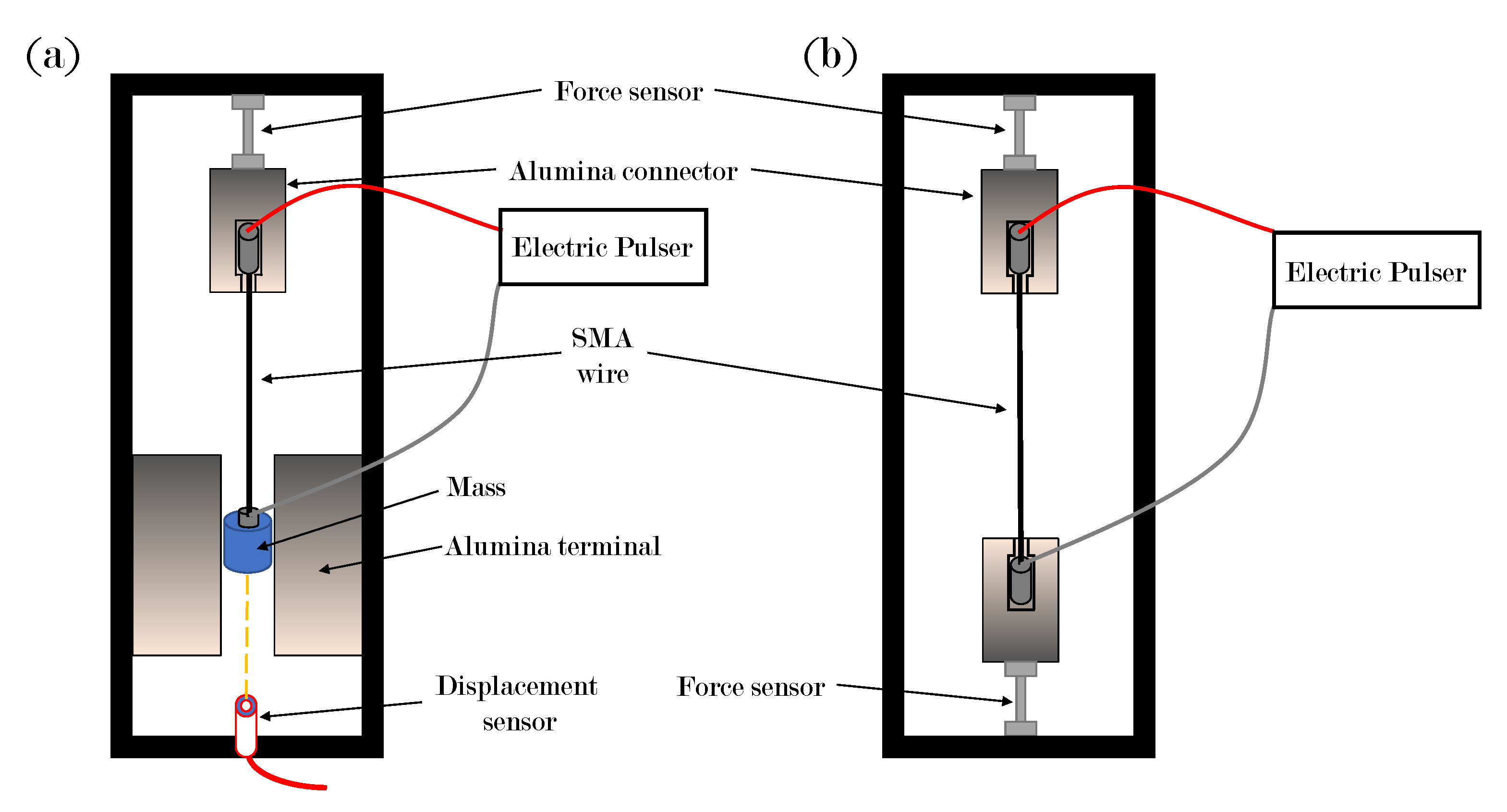
Herein, we will demonstrate that, in the clamp-free configuration, the conditions to which the SMA wire is subjected during the first 1000 μs (determined by the mechanical natural frequency of the actuator) are very similar to those of a wire that is clamped at both ends. The next section surveys typical results of this type of experiments. In particular, experiments in which the wire is clamped at both ends have been used for studying the kinetic law for the phase transformation and the equilibrium stress (as a function of temperature) [38,39]. The latter can be used for evaluating the average stress level at $t\approx 1000$ μs in a clamp-free configuration. A schematic illustration of the mechanical set up of the clamp-clamp experimental configuration is depicted in Figure 3b.

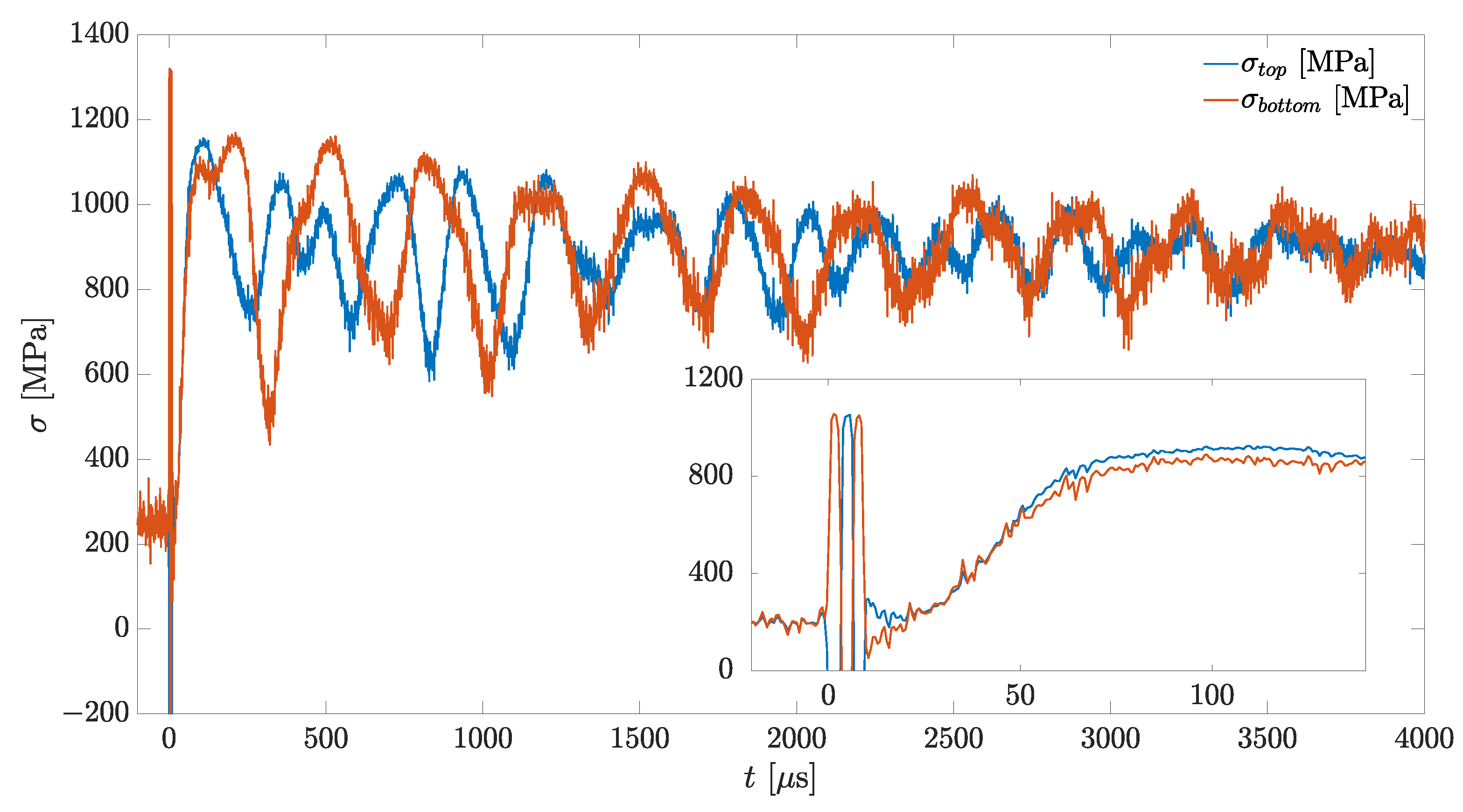
The kinetics and thermodynamics of the high-rate phase transformation under an abrupt heat pulse have been studied using the clamp-clamp mechanical configuration in which the wire was clamped at both ends [34,38]. In this configuration, momentum transfer is negligible and does not restrict the rate of the phase transformation. The curves in Figure 5 present the typical evolution of stress in time, measured by two force sensors, which were attached to both ends of the SMA wire, during the same test. 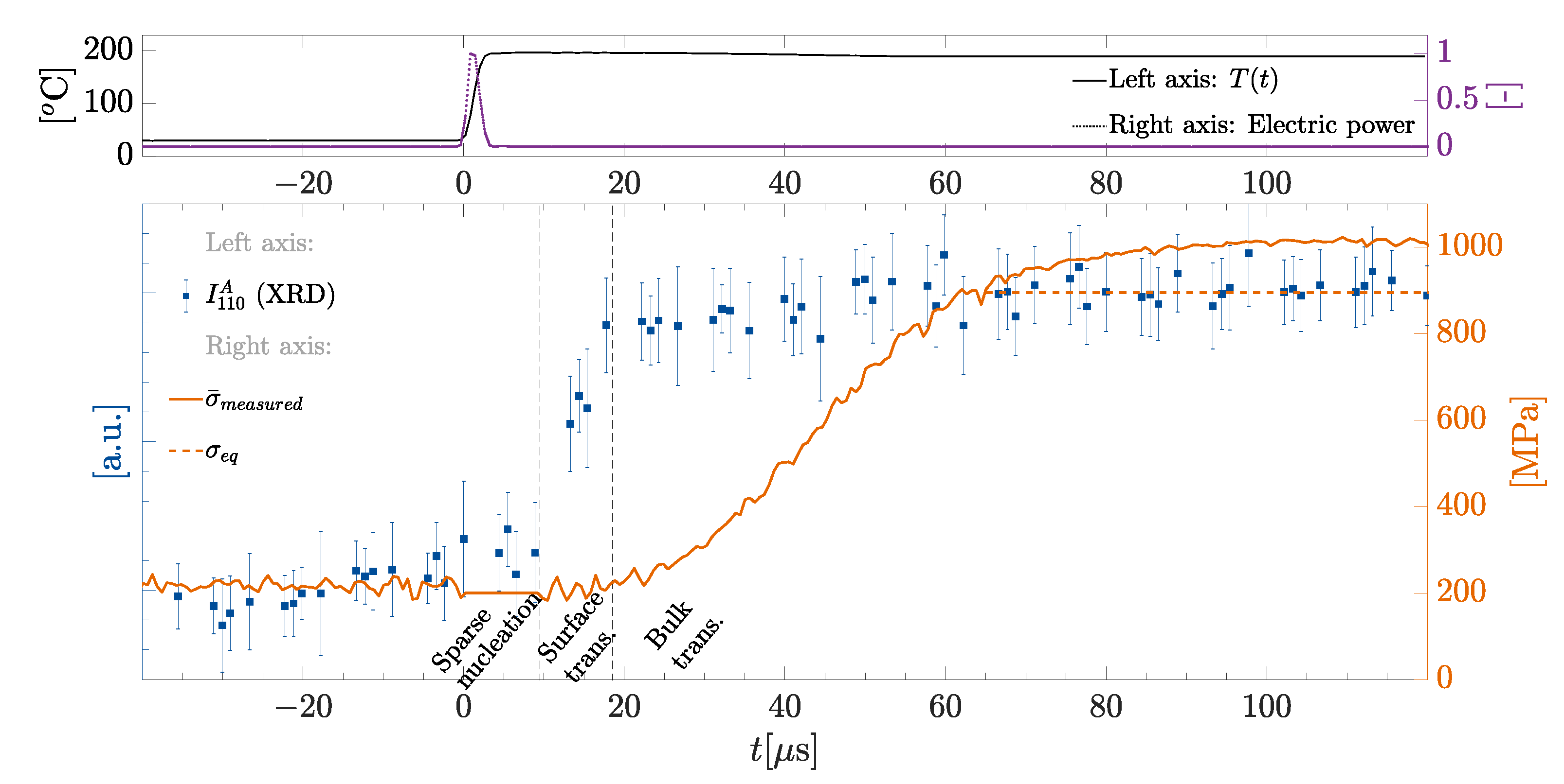Simultaneously, X-ray diffraction patterns were collected from a thin layer, approximately 1 μm in the radial direction, near the surface of the wire [34]. Patterns were collected with a temporal resolution of approximately 1 μs. The volume fraction of austenite is presented by the blue squares in Figure 6, normalized with respect to its mean final value (i.e., mean of plateau after 20 μs).

Two main differences with respect to the stress versus time presented in Figure 4 are observed. First, in Figure 6 prior to the heat pulse the stress is held at a constant predefined stress ${\sigma }_0$ (200 MPa in this test) that is applied by pre-stretching the SMA wire. (The 200 MPa stress, representing the detwinning stress in the Flexinol wires, was determined based on the method specified by Vollach et al. (2016) [33].) Second, after the first stress peak, the force oscillates (see Figure 5) around a plateau value until the vibrations dampen and the stress settles at an equilibrium value, ${\sigma }_{eq}$, denoted by the horizontal dashed line in Figure 6. The increase of the stress decreases the driving force for the transformation to the austenite phase, until at ${\sigma }_{eq}$, a thermodynamic equilibrium between the austenite and martensite phases is achieved. At this stage, the austenite volume fraction, $x_{eq}$, is significantly smaller than unity, indicating that the transformation is incomplete. In that aspect, experiments performed under the clamp-clamp conditions are different than those under the clamp-free conditions, in which the motion of the mass (especially at times larger than the mechanical response of the system) releases the stress and allows the phase transformation to complete.

Measurements at longer time scales (e.g., Figure 5) show that the stress remains constant at ${\sigma }_{eq}$ for 1–2 s and returns to approximately ${\sigma }_0$ upon cooling. This is in contrast with the behavior shown in Figure 4, showing results obtained using the clamp-free configuration, in which the stress decreases to zero within few milliseconds due to the motion of the free end of the wire.

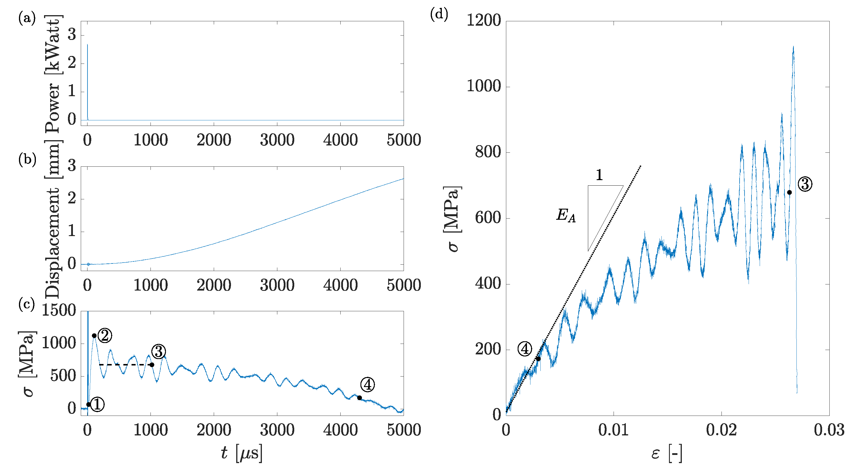
There are several similarities in the behavior of the stress versus time curves presented in Figure 4c and Figure 6 during the first 1000 μs. Both experiments display a dead time $t_{dead}\approx 20$–30 μs between the time at which the heat pulse is applied and the time at which the stress starts rising. After the dead time, in both experiments the stress begins to increase rapidly and reaches a maximum within $t_{rise}\approx 40$–50 μs. The times $t_{dead}$ and $t_{rise}$ are clearly observed in the inset of Figure 5 and Figure 6, which show a zoom-in on the beginning of the test. In addition, both Figure 4 and Figure 5 display force oscillations that are induced by string like-vibrations. In both cases, the force oscillations are not fully harmonic but can still be characterized by a time period $T_{vib}$, which is approximately the same in Figure 4 and Figure 5. Due to the string-like vibrations, at times greater than 100 μs, the stress along the wire is not uniform, as is manifested by the difference between the readings of the two force sensors displayed in Figure 5. Nevertheless, the two curves exhibit the same values of $t_{dead}$, $t_{rise}$, $T_{vib}$, and ${\sigma }_{eq}$ and differ only in the temporary phase of the force oscillations.

The observation that the two force sensors measure an identical value of $t_{dead}$ up to a temporal resolution of $\delta t_{dead}=1$ μs (inset of Figure 5) indicates that, at the macro (mm) scale, the wire responds homogeneously; therefore, the time that it takes for the longitudinal stress waves to travel along the wire has a negligible effect on the characteristic time $t_{dead}$. In addition, the duration of the heat pulse and the time that it takes for the longitudinal stress waves to travel along the connector between the wire and the force sensor are smaller by an order of magnitude than $t_{dead}$. This means that most of the dead time is attributed to a characteristic time of the phase transformation, which was called incubation time $t_0$. The incubation time describes a time interval during which the transformed volume is small so that macroscopic stress changes are negligible.

The microsecond-scale time-resolved XRD study of the transformation [34] showed that the slow response of the macroscopic force in the wire is preceded by a fast, steep rise in the volume fraction of the austenite phase near the surface of the wire (blue squares in Figure 6), indicating the nucleation and formation of a partially transformed martensite-austenitie layer in that region. However, the low macroscopic response implies that this layer is much smaller than the total volume of the wire. Furthermore, their X-ray beam probed a region with a length of approximately 1 mm along the wire axis, performing hundreds of XRD tests at different positions along various wires obtaining highly repeatable results. Dana et al. [34] suggested that during the dead time the nucleation and formation of a cylindrical phase front takes place, and that the following rise time, is the propagation of this front from the periphery of the wire inwards. Unsurprisingly, previous slow [47,48] and high [33] rate studies of Flexinol wires measured strain and temperature changes only at the surface and, therefore, could not observe such effects.

Volkov et al. [35] studied the response of SMA wires at the very first stages, using a configuration in which the wire was completely free of mechanical loads and constrains. The incubation time in their case was approximately 1 μs. This observation is probably attributed to the absence of mechanical loads, constraints, or masses in their experiments, allowing the rapid transformation near the wire surface to induce measurable displacements. Another contribution to the different dead times may be the use of different SMA materials, having different grain sizes and different properties (e.g., a two-way versus one-way shape memory effect).

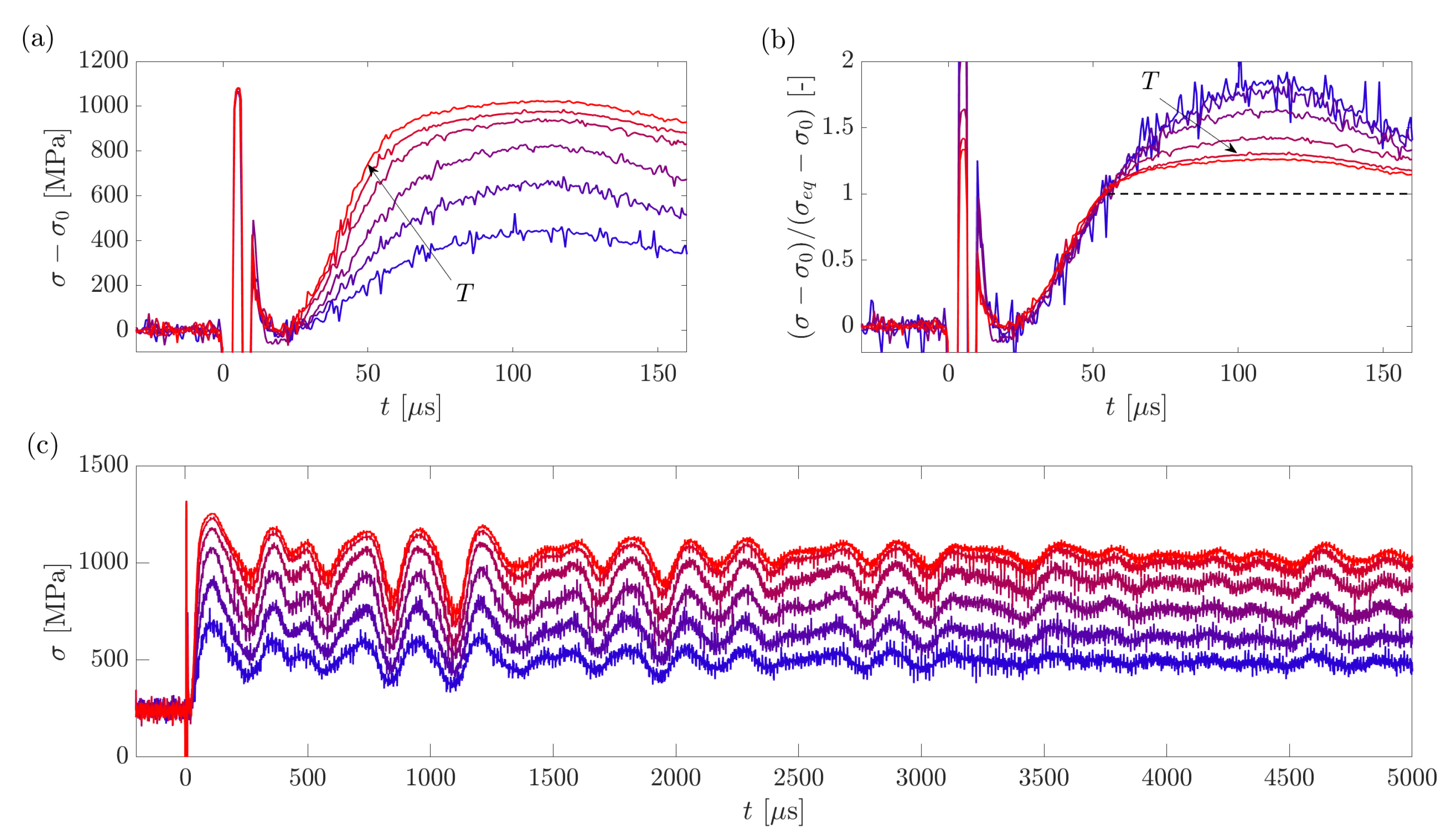
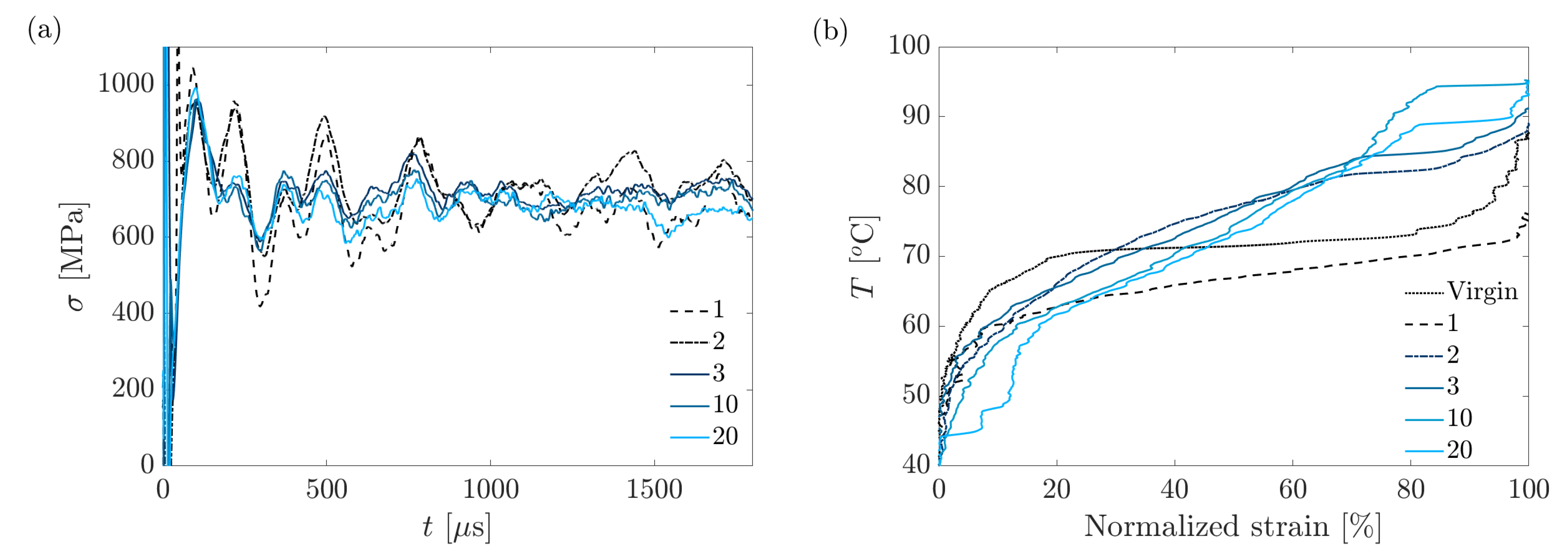
The dependence of the transformation rate on the temperature has been studied by performing sets of tests using the same wire but applying different input energies and in accordance different temperature jumps. The typical results, presented in Figure 7a, show that the rise time does not depend on the temperature. To explain this result, Vollach et al. [38] developed a model for the transformation kinetics during the third stage of the phase transformation (i.e., at $t>t_{dead}$). The main assumption of the model is a linear (overdamped) kinetic law between the rate of change of the austenite volume fraction, $\dot{x}\left(t\right)$, and the thermodynamic driving force for the phase transformation, g,

$$\dot{x}\left(t\right)=\mu g=\mu \left[{\sigma }_{eq}\left(T\left(t\right)\right)-\sigma \left(t\right)\right]{\epsilon }_0,$$

(13)

where $\mu$ is a mobility coefficient.

The wire is clamped at both ends; hence, the overall strain change during the test is approximately zero, i.e.,

$$\left(\frac{\sigma }{E\left(x\right)}-\frac{{\sigma }_0}{E_M}\right)-x\left(t\right){\epsilon }_0+{\epsilon }_p=0.$$

(14)

The first term in Equation (14) represents the change in the elastic strain, where $E\left(x\right)$ is an effective Young’s modulus that depends on the volume fraction, x, and $E_M$ is the Young’s modulus of the martensite phase. Ultrasonic measurements showed that, at high rates, the Young’s moduli of the austenite and martensite phases are almost the same and are approximately equal to 60–70 GPa [45]. The second term in Equation (14) represents the strain change due to the phase transformation, and the last term represents the plastic strain, which was measured and found to be negligible (see discussion in Section 4). Using the approximations that ${\epsilon }_p=0$ and $E\left(x\right)=E_M\equiv E$, the authors obtained an approximate expression for the volume fraction,

$$x=\frac{\sigma -{\sigma }_0}{E{\epsilon }_0}.$$

(15)

The maximal value of x is the equilibrium value $x_{eq}$, which is obtained when $\sigma ={\sigma }_{eq}$. A substitution of typical values in Equation (15) showed that $x_{eq}\approx 0.25$. For this value, the latent heat term in Equation (3) is negligible (typically smaller than 7 K); therefore, the temperature during the clamp-clamp experiments is approximately constant. Thus, ${\sigma }_{eq}\left(T\left(t\right)\right)$ in Equation (13) is approximately constant. Note that this approximation is not valid for the clamp-free configuration, in which $x\left(t\right)$ reaches unity.

The substitution of Equation (15) into Equation (13) provides the first order, linear ordinary differential equation (ODE),

$$\dot{\sigma }+\mu E{\epsilon }_0^2\left(\sigma -{\sigma }_{eq}\right)=0$$

(16)

The solution of Equation (16), together with the initial condition $\sigma \left(t_0\right)={\sigma }_0$, provides a universal normalized expression of the form

$$\frac{\sigma \left(t\right)-{\sigma }_0}{{\sigma }_{eq}-{\sigma }_0}=1-exp\left(-\frac{t-t_0}{\tau }\right),\mathrm{for}t⩾t_0,$$

(17)

where $\tau$ is a basic material property, defined by

$$\tau ={\left(\mu E{\epsilon }_0^2\right)}^{-1}.$$

(18)

The expression in Equation (18) describes the characteristic response time of the phase transformation under all experimental conditions. Note that the only influence of the temperature on $\sigma \left(t\right)$ comes from ${\sigma }_{eq}\left(T\right)$; therefore, the rise time, which is determined by $\tau$, is temperature independent.

Figure 7b presents the measured data presented in Figure 7a in terms of the normalized expression on the left hand side of Equation (17). In this representation, all curves collapse to a single universal curve, and the equilibrium stress, ${\sigma }_{eq}$, is scaled to unity, as depicted by the dashed black line in Figure 7b. Note that the experimental results follow the model prediction only during the rise of the stress. At later times, the string-like vibrations result in oscillations around the model prediction. Additional sets of experiments (not shown in this article) demonstrated that the normalized stress versus time representation is also valid for tests that have been performed on different wires with different diameter and length [34,38]. All these experiments presented approximately the same value of the characteristic time $\tau =28$ μs [38].

The collapse of all experimental measurements, performed under different temperature jumps and various wire lengths and diameters, to a single universal analytical expression, given by Equation (17), indicates that the assumed kinetic law, Equation (13) properly describes the evolution of the phase transformation in the third stage. The physical meanings of this kinetic law, from a material science point of view, are discussed in Refs. [38,46]. In Section 7, we will use this kinetic law to model and simulate the dynamic response in clamp-free experiments.

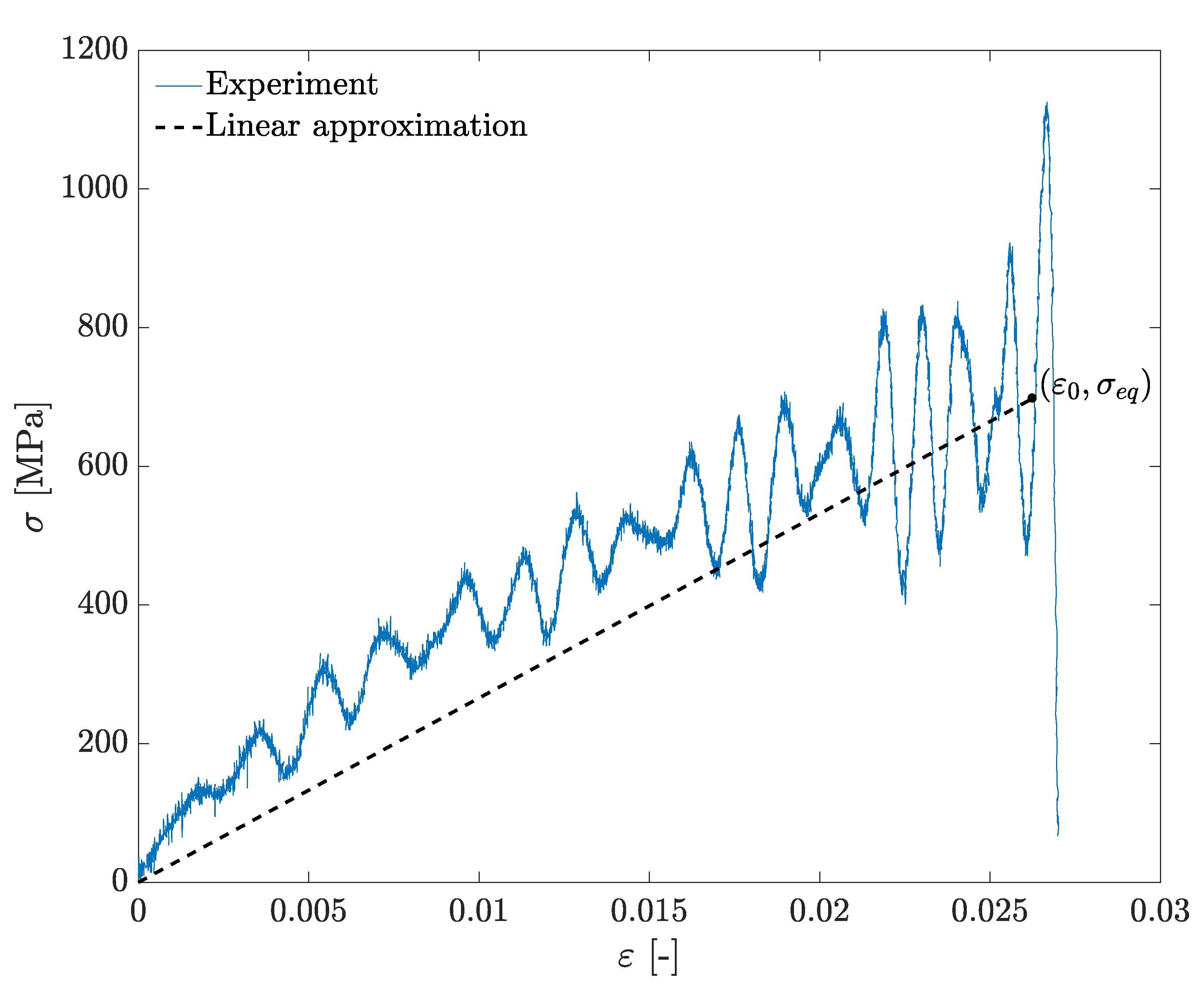
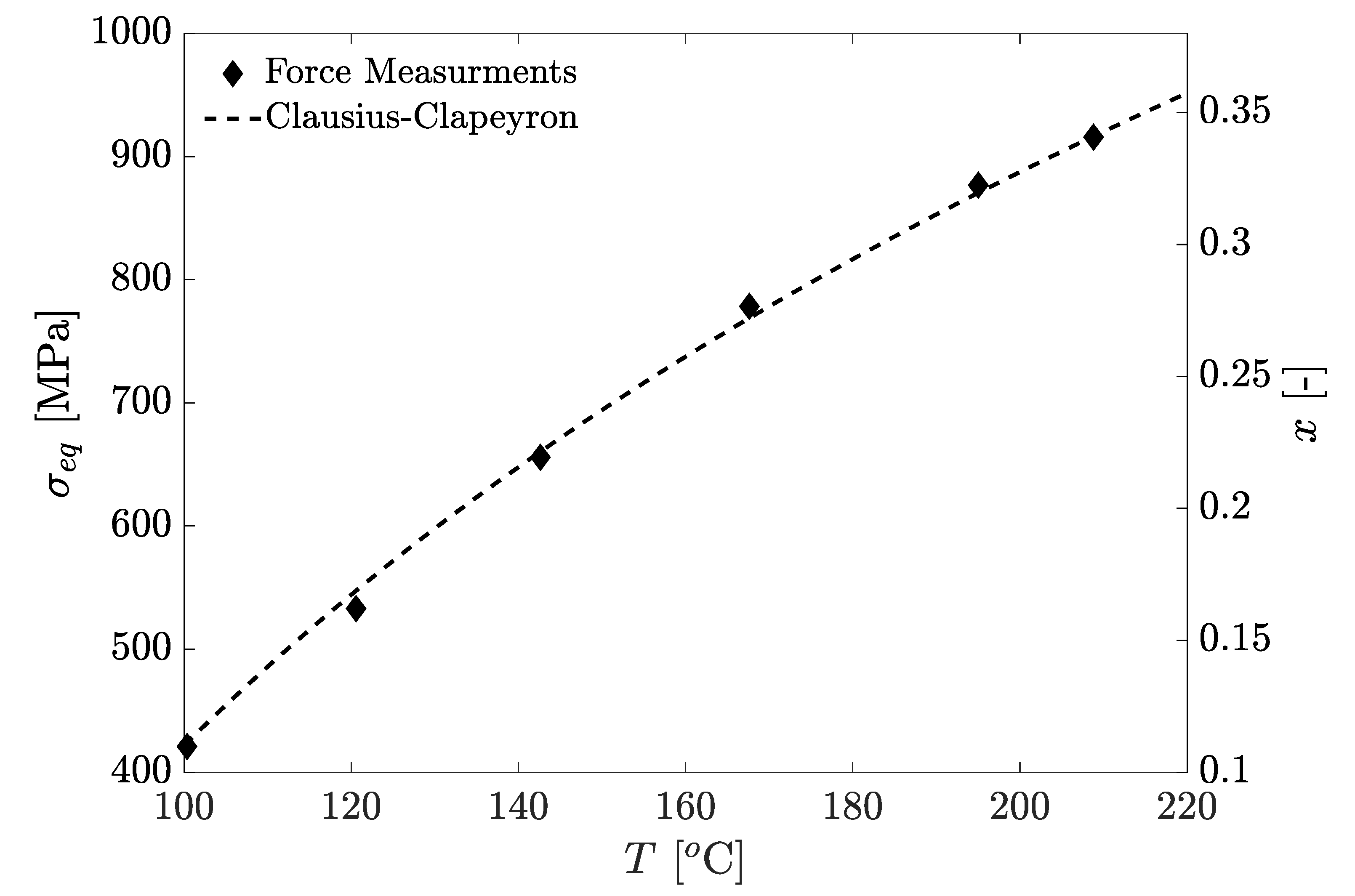
The dependence of the equilibrium stress on the temperature and the austenite volume fraction has been studied in Ref. [39]. The equilibrium stress was evaluated based on the average stress during the time interval of $2.5\mathrm{ms}<t<4$ ms, as shown in Figure 7c. A plot of the equilibrium stress as a function of temperature for a set of experiments, performed on a wire with a diameter of 0.2 mm and a length of 48 mm, is shown by the diamond markers in Figure 8. The right axis in Figure 8 also provides information on the austenite volume fraction, $x_{eq}$, at the equilibrium stress, obtained by substituting the equilibrium stress values into Equation (15).

The experimental results presented in Figure 8 can be partially explained based on the adjusted Clausius-Clapeyron relation as expressed in Equation (2). Integration of this equation provides

$${\sigma }_{eq}=\tilde{\sigma }+\frac{H}{{\epsilon }_0}ln\left(\frac{T}{\tilde{T}}\right),$$

(19)

where $\left(\tilde{T},\tilde{\sigma }\right)$ is a reference point fulfilling the equilibrium conditions, i.e., a martensite to austenite transformation under a constant driving force. The transition temperature, $\tilde{T}$, is not a single value property. Instead, it depends on x and changes between the austenite start, $A_s=\tilde{T}(x=0)$, and austenite finish, $A_f=\tilde{T}(x=1)$, temperatures. We comment that different characterization methods have different sensitivities to the onset and the end of the phase transformation [39].

To evaluate $\tilde{T}$, slow-rate experiments, in which a constant stress was imposed on a clamp-free wire, were performed. Initially, a detwinning stress of approximately 200 MPa (following Vollach et al. (2016) [33]) was imposed on the martensitic wire. Then, a freely hanging mass (equivalent to $\tilde{\sigma }=20$ MPa) was attached to one end of the wire. During the experiment, the wire was slowly heated using a DC current, and the length of the equilibrated wire was measured at each step. Measurements of $\tilde{T}$ versus x under a constant stress of $\tilde{\sigma }=20$ MPa are presented in Figure 9. The results were fitted to a function of the form

$$T\left(x\right)=\left\{\begin{array}{ccc}{T}_2-(T_2-T_1)\exp (-\frac{x}{{\lambda }_1}),\hfill & \mathrm{if}x\left(t\right)\le 0.05,\hfill & \left(20\mathrm{a}\right)\hfill \\ T_4-(T_4-T_3)\exp (-\frac{{\lambda }_2}{1-x}),\hfill & \mathrm{if}x\left(t\right)>0.05,\hfill & \left(20\mathrm{b}\right)\hfill \end{array}\right.$$

where $T_1=24{}^{\circ }$C, $T_2=72{}^{\circ }$C, $T_3=71{}^{\circ }$C, $T_4=88{}^{\circ }$C, ${\lambda }_1=0.073$ and ${\lambda }_2=0.03$. For the analysis of the clamp-clamp experiments, only Equation (20a) was used, as in all these tests $x<0.3$.

A fitting of the equilibrium stress results to the Clausius-Clapeyron Equation (19) is presented by the dashed curve in Figure 8. The curve fits well to the experimental results, showing its efficacy in predicting the evolved equilibrium stress.

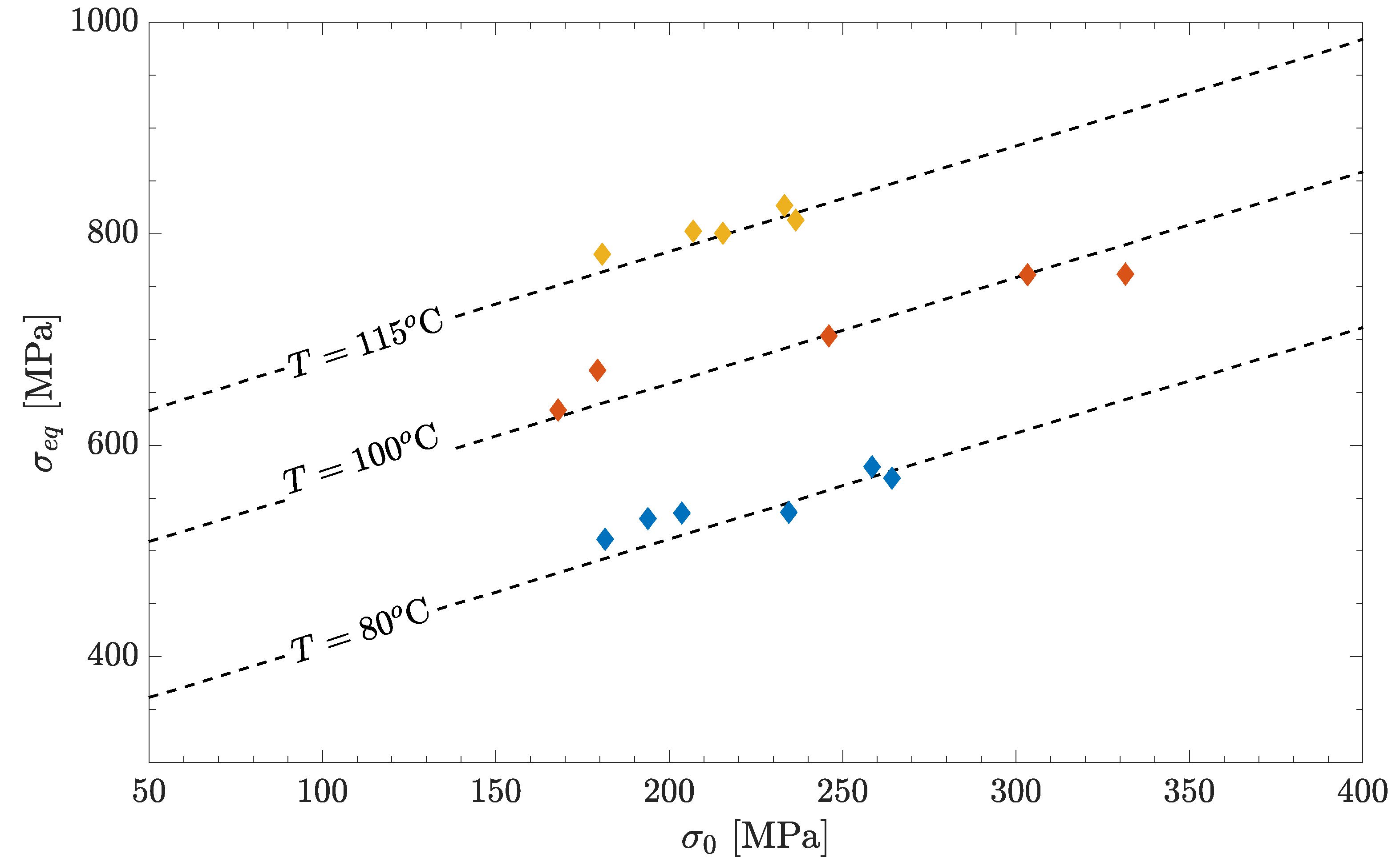
Figure 10 presents measurements of ${\sigma }_{eq}$ versus ${\sigma }_0$ for three different temperatures, $T=80{}^{\circ }$C, $T=96{}^{\circ }$C, and $T=114{}^{\circ }$C, under the clamp-clamp configuration. These measurements were performed by applying the same temperature jump on the same wire, but changing the initial stress, ${\sigma }_0$, that was applied in each test. The different values of ${\sigma }_0$ affected the values of $x_{eq}$ according to Equation (15). The dashed lines presented in Figure 10 are calculated based on Equations (19) and (20a) for various constant values of T. The calculated curves that best fit the measured data are those corresponding to $80{}^{\circ }$C, $100{}^{\circ }$C, and $115{}^{\circ }$C, i.e., negligible difference with respect to the calculated temperature values based on Equation (3). The agreement between the calculated curves and the measured values in Figure 10 is excellent, considering that the only fitted parameters are $T_1$, $T_2$, and ${\lambda }_1$, which were determined based on a different independent experiment, presented in Figure 9.

6. Phenomenological Approximations of the Clamp-Free Actuator Performance

In this section, we deal with the overall actuator performance in terms of key characteristics, such as the energy efficiency and the total actuation time. For example, based on the measured curves, such as those presented in Figure 4 and Figure 6, we determine the energy efficiency and the actuation time. Thus, instead of dealing with the full curves of stress and strain as a function of time, we deal with single-valued characteristics that are not functions of time. By mapping the actuator characteristics as a function of temperature and other parameters, we suggest rough approximations for measures of the actuator performance. These approximations can serve as design tools.

Herein, we focus on the clamp-free setup, in which one end of the NiTi wire is clamped, while the other end is connected to a mass that is free to move with negligible friction. In all measurements presented in this section, the duration of the electric heating pulse is shorter than 4 μs, which means that the wire reaches the maximal temperature before the phase transformation begins.

6.1. Energy Efficiency

Energy efficiency is a crucial merit for any actuator. As discussed in Section 2, SMA actuators activated by a fast heating pulse provide better energy efficiency with respect to slow rate SMA actuators. To study the energy efficiency, we have to evaluate both the input electrical energy and the work performed by the SMA wire. The input energy is evaluated by measuring the current and voltage over the wire using a parallel circuit with a large resistor. The work output is evaluated based on the kinetic energy of the mass at the end of the actuation, i.e., when the stress in the NiTi wire returned to its initial value and the mass continues moving in free-flight. For this purpose, the maximal velocity can be evaluated by fitting a linear function to the measured displacement versus time signal, in an interval of approximately 0.2 ms after the stress returned to zero.

Figure 11 presents the specific output energy $U_{out}$ as a function of the specific input energy $U_{in}$. At energies below $U_{in}=0.8$ J/mm${}^3$, there is an approximately linear relation between the input and output energies. Above this point, the output energy is almost indifferent to the input energy. An input energy of $U_{in}=0.8$ J/mm${}^3$, thus, represents the optimal operation conditions, as the efficiency is maximal at this point, at a value of approximately 3.5% (as evident from the dashed lines signifying different efficiencies).

The upper x-axis presented in Figure 11 represents the temperature immediately after the heat pulse, calculated based on Equation (3) with the substitution of $x=0$, i.e., assuming that the wire is still in the martensite phase. At the optimal point where $U_{in}=0.8$ J/mm${}^3$, the temperature of the wire is approximately $170{}^{\circ }$C. Interestingly, rapid heating to a temperature of $120{}^{\circ }$C, which is reduced, due to the latent heat, to a temperature of approximately $A_f=90{}^{\circ }$C at the end of the phase transformation, provides just half of the maximal energy efficiency.

The temperature after the pulse heating depends on the ambient temperature $T_R$ (see Equation (3)). Certain applications may require operation at a wide range of ambient temperatures. In these cases, the input energy $U_{in}$ can be adapted based on the measured $T_R$. Alternatively, the value of $U_{in}$ can be chosen such that, even under the smallest possible value of $T_R$ the wire will be heated to above $170{}^{\circ }$C. In this case, a higher value of $T_R$ will result in a temperature above $170{}^{\circ }$C after the pulse. Figure 11 demonstrates that, at temperatures above $170{}^{\circ }$C, the output energy is approximately constant, even if the temperature rises to $280{}^{\circ }$C. It is important to note that there was no sign of failure or degradation in the SMA performance following the use of the highest energy (we applied an actuation order of alternating high-low-high energies).

In summary, based on the above, we suggest that a practical rapid actuation design should use an input energy slightly above the optimal point, e.g., $U_{in}=0.9$ J/mm${}^3$ (corresponding with approximately $190{}^{\circ }$C). This value ensures insensitivity of the output energy to small variations (e.g., wire geometry, supplied power, initial temperature), does not damage to the SMA, keeps the efficiency close to the optimal conditions (larger than 3%) and assures the maximal energy output possible.

6.2. Duration of Actuation

One of the main reasons to use rapid heating is to achieve a rapid actuation. The duration of the actuation, $t_{actuation}$, which is defined as the time during which the stress applied by the NiTi wire is larger than zero, therefore, is a key design parameter.

Herein, we present a rough approximation of the actuation duration, expressed in terms of known parameters, that enables designers to estimate the duration of actuation before doing the actual tests. The approximation is considered by replacing the complicated stress strain curve with a straight line, as demonstrated in Figure 12. The line connects the point $({\epsilon }_0,{\sigma }_{eq})$, obtained at a short time after the heating pulse (approximately 100 μs; see discussion in Section 4), and the origin, obtained at $t=t_{actuation}$. The straight line represents the mechanical response of an effective spring with the stiffness $k_{eff}$ given by

$$k_{eff}=\frac{{\sigma }_{eq}A}{{\epsilon }_0{L}_0}.$$

(21)

Thus, the complicated dynamic behavior of the actuator can be approximated by a spring-mass model with a natural frequency ${\omega }_{eff}=\sqrt{k_{eff}/m}$, where m is the total mass connected to the free end of the wire. Assuming that the point $({\epsilon }_0,{\sigma }_{eq})$ is reached in a time that is negligible with respect to the overall actuation duration, $t_{actuation}$, the latter is approximately equal to a quarter of the time period of the natural frequency, i.e.,

$$t_{actuation}=\frac{\pi }{2{\omega }_{eff}}=\frac{\pi }{2}\sqrt{\frac{m}{k_{eff}}}.$$

(22)

Substituting Equation (21) into Equation (22) and using $A=\pi d^2/4$, we obtain

$$t_{actuation}=\pi \sqrt{\frac{m{\epsilon }_{0}L}{{\sigma }_{eq}\pi d^2}}.$$

(23)

The value of ${\sigma }_{eq}$ can be approximated based on Equations (19) and (20a,b), as discussed in Section 5.

Figure 13 compares the estimated actuation duration, based on Equation (23) with the actual measured actuation duration. All experimental results, taken with a different wire length, mass, and initial strain, sit approximately on a straight line with a slope of unity, signifying that the estimated actuation duration is equal to the measured one. The overall agreement of the results with this line is very good, especially for the experiments denoted by the triangular markers, which were conducted using the suggested input energy of $U_{in}=0.9$ J/mm${}^3$.

6.3. Repeatability and Fatigue

Repeated cycles of rapid actuation are prone to eventually degrade the performance of the actuator. However, lifetime may vary at different actuation conditions. The two main factors that can accelerate degradation are the high temperatures and the resulting high evolved stress. The rapid actuation involves both factors at levels that greatly exceed conventional slow SMA actuations. Specifically, the typical stress peak surpasses 1.2 GPa for a period of less than 50 μs (as evident in Figure 4 and Figure 7), and the recommended actuation temperature is almost 100 ${}^{\circ }$C above the $A_f$.

One possible degradation mechanism is plastic deformation. The effect of the unrecoverable plastic strain was measured and was found to be minor when a rapid heating pulse is applied, even in tests at which high temperatures and stress values were obtained. Specifically, in all tests, the plastic strain was an order of magnitude smaller than the transformation strain, ${\epsilon }_0$. Surprisingly, this was found to be true for both the clamp-free and the clamp-clamp configurations, which were shown to behave similarly during the initial 100 μs of actuation. The main reason is that stress evolution in the wire stops the transformation from proceeding when the equilibrium stress is reached, effectively decreasing the driving force for the transformation [38,46]. Thus, the austenite fraction in the clamp-clamp configuration remains at the constant value until cooling, while, in the clamp-free configuration, it continues to evolve with the decrease of stress in the wire, as shown in Figure 4 and Figure 12. Slow-rate applications involving continuous mechanical or thermomechanical loading of superelastic NiTi were shown to exhibit various plastic deformation mechanisms and shape setting effects [48,50,51]. Albeit, these situations are not relevant to the case of pulse heating, as discussed in this work.

In this section, we check two degradation effects that are directly relevant to the actuator performance. First, we present a set of consecutive tests performed on the same wire and check the repeatability of the performances. Secondly, we evaluate the effect of the pulse tests on the transition temperature by measuring it (under slow heating with a small applied stress) between consecutive high-rate pulse tests.

A single clamped-clamped wire was activated for 20 consecutive cycles, all carried with a pulse energy of $U_{in}=0.83$ J/mm${}^3$, and an initial stress of 200 MPa. The clamp-clamp configuration is expected to produce more damage than the clamp-free experiment because the former exhibits stress and temperature values that are always equal or larger (the plateau stress lasts for a longer period, and the incomplete transformation reduces the loss to latent heat).

Figure 14a presents the stress profiles of selected actuation cycles as a function of time. The first two cycles show a different behavior than the rest. This effect is the conditioning or training effect that is well known for slow actuations. Due to this effect, throughout this research the first couple of actuations of virgin wires were always ignored. Results of cycles 3 to 20 indicate that there is no visible change in the stress profile, suggesting that there is no degradation in the performances of the wire.

The phase transformation temperature following each test was studied by the controlled slow heating of the SMA wire and a measurement of the accompanied change in its length. In this experimental setup, the wire is subjected to a small stress, just to the level required to keep it straight during the test. Figure 14b shows the resulting slow heating profiles after each of the experiments presented at Figure 14a. The strain profiles clearly exhibit that the wire is indeed trained after the second pulse, with the behavior following it mostly consistent with the third pulse. Notice that the ‘virgin’ (dotted) curve represents the profile conducted prior to the first rapid actuation (i.e, over a virgin wire). The profiles following the second pulse share a similar strain-temperature profile and appear to have a more uniform progression of transformation. In particular, there was no significant change in the austenite start $A_s$ and finish $A_f$ temperatures. In summary, stress versus time profiles that followed the second actuation and their subsequent strain recovery versus temperature profiles show no evidence of cumulative damage or degradation of wire performance for the rapid actuation mode.

7. Detailed Design Tool: Full Dynamic Simulations of Clamp-Free Actuators

In this section, we construct a model describing the thermo-mechanical dynamics of high-rate SMA actuators, albeit still ignoring the string-like force vibrations. This model enables us to simulate the displacement and stress as a function of time. Such simulations can be used as a design tool, to investigate the effects of operation parameters, such as the duration of the electric pulse, without the need to run repeated sets of tests. Moreover, the simulations shed light on variables that are not directly measured during the tests, such as the austenite volume fraction and the temperature.

Herein, we model the dynamics of a clamp-free actuator. The model accounts for the kinetic law for the phase transformation and the non-linear response of SMA. We formulate the ODE for the dynamic response of the actuator. In particular, we identify three characteristic times that affect the dynamics of the actuation process: the characteristic time of the heat pulse, ${\tau }_e$; the characteristic time of the phase transformation, $\tau$; and the time period $\pi /2{\omega }_{eff}$ associated with the natural frequency, ${\omega }_{eff}$, of the mechanical response of the system (as discussed in Section 6.2). A preliminary discussion of these characteristic times has already been presented in Section 1 (see Table 1) and Section 2.3.

We validate the simulation procedure by demonstrating the agreement between the calculated simulations and the experimental results, taken with ${\tau }_e\sim 1\mathsf{\mu }s\ll \tau$. Then, we use our model to obtain predictions that have not been tested experimentally. In particular, we perform a set of simulations to study the effect of ${\tau }_e$ on the actuator performance. As explained in Section 3, there is an incentive to use larger values of ${\tau }_e$ with an aim of reducing the required voltage. On the other hand, too large values of ${\tau }_e$ result in a smaller work output and longer actuation duration, thus diminishing the actuator performance. Our simulations reveal the desired range for ${\tau }_e$, along which the actuator performance is optimal.

7.1. Model Formulation

To account for the evolution of the dynamics of the SMA actuator, we formulate a set of equations, both algebraic and differential, describing the behavior of the wire as a function of time (see

Table 2. Collection of the main variables, equations and parameters used in the formulation of the model.

Variable	Description	Variable	Description
$\sigma \left(t\right)$	Stress [Pa]	$T\left(t\right)$	Temperature [K]
$x\left(t\right)$	Volume fraction [-]	t	Time [s]
$u\left(t\right)$	Displacement [m]
(#)	Equation	(#)	Equation
(3)	$U_{in}\left(t\right)=\rho C_p[T\left(t\right)-T_R]+Hx\left(t\right)+Q\left(t\right)$	(18)	$\tau ={\left(\mu E{\epsilon }_0^2\right)}^{-1}$
(4)	$F=\sigma A=F_0+ku+m\ddot{u}$	(19)	${\sigma }_{eq}=\tilde{\sigma }+\frac{H}{{\epsilon }_0}ln\left(\frac{T}{\tilde{T}\left(x\right)}\right)$
(9)	$E_{in}=\frac{1}{2}C{V}_0^2$	(20a)	$\tilde{T}\left(x\right)=T_2-\left(T_2-T_1\right)exp\left(-\frac{x}{{\lambda }_1}\right),\mathrm{if}x\left(t\right)⩽0.5$
(10)	${\tau }_e=\frac{1}{2}{R}_{tot}C$	(20b)	$\tilde{T}\left(x\right)=T_4-\left(T_4-T_3\right)exp\left(-\frac{{\lambda }_2}{1-x}\right),\mathrm{if}x\left(t\right)>0.5$
(13)	$\dot{x}\left(t\right)=\mu \left[{\sigma }_{eq}\left(T\left(t\right)\right)-\sigma \left(t\right)\right]{\epsilon }_0$
Parameter	Description	Parameter	Description
H	Latent heat, 156,560,850 [J/m${}^3$].	$\tilde{\sigma }$	Reference stress, 20 [MPa].
$C_p$	Heat capacity, 837 [J/kg K].	$\tilde{T}\left(x\right)$	Reference transformation temperature, [K].
$\rho$	Density, 6450 [kg/m${}^3$].	m	Actuated mass, [kg].
$T_R$	Room temperature, 298 [K].	g	Gravitational acceleration, 9.81 [m/s${}^2$].
${\tau }_e$	Pulse rise time, [s].	${\omega }_0$	Natural mechanical frequency of wire, [s${}^{-1}$].
$\tau$	Characteristic time of the phase transformation, 28 [μs].	${\omega }_s$	Natural mechanical frequency of spring, [s${}^{-1}$].
$t_1$	Minimal time to complete transformation, [s].	${\omega }_{eff}$	Effective natural mechanical frequency, [s${}^{-1}$].
E	Young’s modulus, 60 [GPa].	k	Spring stiffness, [Pa m].
${\epsilon }_0$	Transformation (detwinning) strain, [-].	$F_{ext}$	External force, [N].
$L_0$	Wire length (austenite), [m].	$V_0$	Applied voltage, [V].
A	Wire cross-section, [m${}^2$].	$U_0$	Energy density, [J/mm${}^3$].
$R_{tot}$	Total resistance of the system, [$\mathsf{\Omega }$].	$E_{in}$	Input electrical energy, [J].
C	Discharged capacitance, [F].	$\mu$	Mobility coefficient, [m s/kg].
$T_1$	297 [K], see Section 5.	$T_4$	361 [K], see Section 5.
$T_2$	345 [K], see Section 5.	${\lambda }_1$	0.073 [-], see Section 5.
$T_3$	344 [K], see Section 5.	${\lambda }_2$	0.03 [-], see Section 5.

). A close examination of the main concepts presented in the previous sections reveal that three main variables govern the problem, the stress in the wire, $\sigma \left(t\right)$, the displacement of the mass at the end of the wire, $u\left(t\right)$, and the mean volume fraction of austenite in the wire, $x\left(t\right)$. However, the existence of linear relations between these variables allow us to reduce the problem to a system of only two of the variables, and the third is obtained via substitution.

The following model is based on equations that have been developed and presented in previous sections. For convenience, these equations are rewritten in Table 2.

7.1.1. Kinetics of the Transformation

To account for the kinetics of the transformation, we follow the suggested linear kinetic law, Equation (13), presented in Section 5. The mobility coefficient, $\mu =1/\left(\tau E{\epsilon }_0^2\right)$, is obtained from Equation (18), with the material property $\tau =28$μs, as found in Ref. [38]. However, we no longer consider the equilibrium stress to be an empirical property of the experiment. Instead, it is calculated using Equation (19), where $\tilde{\sigma }=20$ MPa is the parameter used in the empirical determination of the transformation temperature $\tilde{T}\left(x\right)$ presented in Figure 9, and $T\left(t\right)$ is the instantaneous temperature of the wire obtained from Equation (3),

$$T\left(t\right)=T_R+\frac{U_{in}\left(t\right)-Hx\left(t\right)}{\rho Cp},$$

(24)

with the wasted heat term, $Q\left(t\right)$, neglected. The input energy is modelled as the integral of the power pulse up to time t,

$$U_{in}=U_0\left(1-exp\left(-\frac{t}{{\tau }_e}\right)\right),$$

(25)

where $U_0$ is the energy per unit volume supplied to the wire, chosen by the user. A substitution of Equation (10) into Equation (9) provides

$$U_0=\frac{E_{in}}{A{L}_0}=\frac{{\tau }_e{V}_0^2}{A{L}_0{R}_{tot}},$$

(26)

indicating that choosing a larger value of ${\tau }_e$ enables us to use a lower voltage, $V_0$, while still maintaining the same (required) value of $U_0$. In the following simulations, we consider the energy density, $U_0$, as a constant parameter, while studying the effect of changing the characteristic heating time, ${\tau }_e$.

The transition temperature as a function of the instantaneous volume fraction, $\tilde{T}\left(x\right)$, is provided using the empirical fitted functions in Equation (20a,b). Substituting Equations (19) and (24) into Equation (13), we obtain the ordinary differential equation

$$\dot{x}\left(t\right)=\frac{1}{\tau E{\epsilon }_0}\left[\frac{H}{{\epsilon }_0}ln\left(\frac{T_R}{\tilde{T}\left(x\right)}+\frac{U_{in}\left(t\right)-Hx\left(t\right)}{\rho C_p\tilde{T}\left(x\right)}\right)+\tilde{\sigma }-\sigma \left(t\right)\right].$$

(27)

This equation, which is based on the linear kinetic law proposed in Section 5, provides a governing equation for the rate of the evolution of the austenite volume fraction in time, i.e., the progression of the phase transformation in the wire.

7.1.2. Force Equilibrium and Kinematics

Considering a vertical actuation of a mass m, the sum of forces acting on the wire, Equation (4), yields an expression for the stress in the wire,

$$\sigma \left(t\right)=\frac{m\ddot{u}\left(t\right)+ku\left(t\right)+mg+F_{ext}}{A},$$

(28)

where $F_{ext}$ is some constant external force acting on the wire (e.g., due to the initial pre-elongation of a spring with stiffness k).

The displacement of the mass as a function of the austenite volume fraction, $x\left(t\right)$, and the stress in the wire, $\sigma \left(t\right)$, is expressed by

$$\frac{u\left(t\right)}{L_0}=\epsilon (x=0,t=0)-\epsilon (x,t),$$

(29)

where

$$\epsilon (x=0,t=0)={\epsilon }_0+\frac{1}{E}\left(\frac{mg+F_{ext}}{A}\right)$$

(30)

is the strain in the wire before the heat pulse, and

$$\epsilon (x,t)=\left(1-x\left(t\right)\right){\epsilon }_0+\frac{\sigma \left(t\right)}{E}$$

(31)

is the strain in the wire at time t. In Equation (31), we neglect thermal expansion, which for NiTi subjected to a temperature change of ∼100 ${}^{\circ }$C may result in a strain on the order of ${10}^{-3}$, smaller by an order of magnitude than ${\epsilon }_0$. In both Equations (30) and (31), the first term represents the transformation strain and the second term represents the elastic strain. In these equations, the plastic strain is again considered negligible, and a constant elastic modulus, E, for the two phases is assumed (see discussion in Section 5). Substituting Equations (30) and (31) into Equation (29), we obtain

$$\frac{u\left(t\right)}{L_0}=x\left(t\right){\epsilon }_0-\frac{1}{E}\left(\sigma \left(t\right)-\frac{mg+F_{ext}}{A}\right).$$

(32)

Substituting Equation (28) into Equation (32), we obtain

$$\ddot{u}+({\omega }_0^2+{\omega }_s^2)u\left(t\right)={\omega }_0^2{L}_0{\epsilon }_{0}x\left(t\right),$$

(33)

where ${\omega }_0^2=EA/L_{0}m$ and ${\omega }_s^2=k/m$ are the mechanical natural frequencies of the wire and the spring, respectively. The addition of these frequencies, ${\omega }_{eff}=\sqrt{{\omega }_0^2+{\omega }_s^2}=\sqrt{(EA/L_0+k)/m}=\sqrt{k_{eff}/m}$, thus, can be considered as an equivalent system of parallel springs with stiffness $k_{eff}$ and natural frequency ${\omega }_{eff}$.

The obtained Equations (27), (33) and either (28) or (32), is a system of algebraic-differential equations. However, it can be easily reduced to a simpler system of ODEs by eliminating $\sigma \left(t\right)$ and solving an equivalent problem for $x\left(t\right)$ and $u\left(t\right)$. Substituting Equation (32) into Equation (27), we obtain

$$\dot{x}\left(t\right)=\frac{1}{\tau E{\epsilon }_0}\left[\frac{H}{{\epsilon }_0}ln\left(\frac{T_R}{\tilde{T}\left(x\right)}+\frac{U_{in}\left(t\right)-Hx\left(t\right)}{\rho C_p\tilde{T}\left(x\right)}\right)+\tilde{\sigma }-x\left(t\right)E{\epsilon }_0+\frac{u\left(t\right)}{L_0}E-\frac{mg}{A}-\frac{F_{ext}}{A}\right].$$

(34)

Finally, substituting Equation (33) into (34), we obtain a third order ODE for $u\left(t\right)$. The equation is evolved numerically using the Matlab ‘ODE113’ subroutine, and the solution is substituted back into Equations (28) and (32) to obtain $x\left(t\right)$ and $\sigma \left(t\right)$. The third order equation, requires the three initial conditions,

$$\begin{array}{c}\hfill u\left(0\right)=0,\end{array}$$

(35a)

$$\begin{array}{c}\hfill \dot{u}\left(0\right)=0\end{array}$$

(35b)

$$\begin{array}{c}\hfill \ddot{u}\left(0\right)=0\end{array}$$

(35c)

Equation (35a) represents a zero initial displacement. Equation (35b) represents the zero initial slope at the beginning of the transformation, similar to the behavior of the clamp-clamp setup (see discussion in Section 4). Equation (35c) is obtained by substituting the expression for the initial stress $\sigma \left(0\right)=(mg+F_{ext})/A$, along with Equation (35a), into Equation (28).

7.2. Actuator Response after the Phase Transformation Has Ended

The kinetic law, (13), applies only to the situation in which $T\left(t\right)>\tilde{T}\left(x\right)$ and $x\left(t\right)<1$. The former is an inherent condition of the high-driving-force regime, applying throughout the simulations presented in this work. However, at certain conditions the transformation completes before the stress completely relaxes or a complete recovery of the strain is achieved. This may occur when the rapid transformation kinetics supersede the elastic relaxation of the wire. To deal with this issue, we identify the time $t_1$, at which $x\left(t\right)$ reaches unity and find the values of $u\left(t_1\right)$ and $\dot{u}\left(t_1\right)$. For $t>t_1$, we calculate the evolution of stress and displacement by assuming a linear elastic response of the wire, until the stress is relaxed to its initial value. For this purpose, we fix the value of $x=1$ and use only Equations (28) and (33). These have an analytic solution of the form.

$$u(t>t_1)=\frac{{\omega }_0^2}{{\omega }_{eff}^2}{L}_0{\epsilon }_0+\left(u\left(t_1\right)-\frac{{\omega }_0^2}{{\omega }_{eff}^2}{L}_0{\epsilon }_0\right)cos\left[{\omega }_0\left(t-t_1\right)\right]+\frac{1}{{\omega }_{eff}}\dot{u}\left(t_1\right)sin\left[{\omega }_0\left(t-t_1\right)\right].$$

(36)

8. Simulation Results

8.1. Comparison with a Typical Experiment

Herein, we test the validity of our proposed model by comparing the obtained results to the typical clamp-free experiment presented in Section 4. This experiment did not include any external forces, i.e., $F_{ext}=0$, and the mass was not connected to a spring, i.e., $k=0$. Thus, the natural frequency of the mechanical response of the system is directly proportional to the stiffness of the wire, i.e., ${\omega }_{eff}={\omega }_0$.

Table 2 lists the values of material properties that were used for all the simulations. The parameters applied in this section were taken to directly match those in the presented experimental setup. These parameters are: $d=0.381$ mm, $L_0=93$ mm, $U_0=0.55$ J/mm${}^3$, ${\tau }_e=6.5$μs, $m=0.27$ kg, and ${\epsilon }_0=0.027$ (measured before the pulse using the method reported in Ref. [33]).

Results of the simulation of our typical experiment are shown in Figure 15. The input energy discharged into the wire is shown to increase much faster than the austenite volume fraction, $x\left(t\right)$ (Figure 15a,b). Thus, the driving force for the transformation is provided faster than the kinetics of the transformation. This is further demonstrated by the wire temperature, $T\left(t\right)$, which is greater than the transformation temperature, $\tilde{T}\left(x\right)$, throughout the experiment (Figure 15c,d).

A comparison of our simulation to a typical experiment is presented in Figure 16. The evolutions of both displacement and stress in time are present in the respective top and bottom panels on the left. The displacement of the mass in our simulation, dashed red curve in Figure 16a, is shown to obtain a similar trajectory to that measured in the experiment. The experiment is considered to end when the wire fully shortens by the value of its initial strain (represented by the horizontal dashed black line), achieved in both curves at approximately 4650 μs. Disagreement between the displacement curves is assumed to be owed to some viscous friction acting on the alumina terminal (guiding the straight path of the mass [33]) during the motion of the wire (see illustration in Figure 3a). The end of the transformation is observed in Figure 15b, when the austenite volume fraction reaches unity, i.e., $x\left(t\right)=1$, at approximately 4300 μs, corresponding to the estimated value of point ④ in Figure 4c.

The stress in our simulation is shown to predict the equilibrium stress evolved in the system, dashed horizontal line in Figure 16b, and holding this value for approximately the initial 1000 μs. Point ② is not reached in the simulation since the string-like vibration is not captured by our model. The simulation then follows the mean path of the oscillating experimental curve, in which the stress slowly decreases, releasing mechanical constraints from the wire and allowing the transformation to proceed, evident from the corresponding increase in $x\left(t\right)$ in Figure 15. At $t\approx 4300$μs, the transformation completes and the wire elastically relaxes any residual stress during the following 350 μs. The spring-like elastic relaxation of the wire is demonstrated by the linear slope corresponding to the elastic modulus of the transformation in Figure 16c showing the stress-strain curve during the experiment.

8.2. Effect of Characteristic Pulse Length

We study the effect of the characteristic rise-time of the electric pulse, ${\tau }_e$, on the dynamics of a clamp-free actuator, i.e., a wire attached to a freely hanging mass, excluding the influence of external forces or springs, i.e., $F_{ext}=k=0$. Herein, we consider a wire with diameter $d=0.2$ mm, length $L_0=50$ mm, and initial strain ${\epsilon }_0=0.03$. The hanged mass is $m=0.1$ kg, and an energy density of 0.9 J/mm${}^3$ is applied. All other material properties are the same as those presented in Section 8.1 and Table 2. For this simulated case, $\pi /2{\omega }_{eff}=2.6$ ms is much larger than $\tau =28$μs.

Figure 17 shows simulated results for three different orders of magnitude of the pulse rise time, ${\tau }_e\in [{10}^{-6},{10}^{-4},{10}^{-3}]$ s. When the pulse is short enough, i.e., ${\tau }_e\ll \tau \ll \pi /2{\omega }_{eff}$, the wire is fully heated well before the phase transformation evolves, at a time-scale proportional to $\tau$, as evident from Figure 15. Figure 17b shows that the stress versus time curves approximately coincide, except for the rise time, which approximately scales as ${\tau }_e+\tau$.

Figure 17g,h show that, at short time scales, increasing values of ${\tau }_e$ achieve a respectively decreasing maximal temperature, probably owing to the latent heat uptake of the commenced transformation. In all cases, a full austenitic state, i.e., $x\left(t\right)=1$ is achieved (Figure 17f), as well as the mass displacing by the full amount set by the initial strain and the wire length, ${\epsilon }_0{L}_0$, similar to Figure 16a. However, rise-time values obeying ${\tau }_e\gtrsim \pi /2{\omega }_{eff}$ did not achieve the maximal possible stress (e.g., Figure 17b), indicating a decrease in energy output efficiency. Moreover, the rightmost curve in Figure 17f, i.e., ${\tau }_e={10}^{-3}\mathrm{s}\approx \pi /2{\omega }_{eff}$, achieved a full transformation at approximately $t=3100$ μs, well before its energy curve in Figure 17d saturated, implying that the energy transferred after that point is wasted on increasing the temperature of the fully austenitic wire (evident from the continued rise in temperature in Figure 17h at $t>3100$ μs).

In general, it can be concluded that Figure 17a,c,e,g show the effect of the characteristic heating time, ${\tau }_e$, in the limit where it is greater than the characteristic phase transformation time, $\tau$, yet smaller than the mechanical response time of the system, $\pi /2{\omega }_{eff}$. Figure 17b,d,f,h then show the effect of ${\tau }_e$ in the limit where it is on the order of $\pi /2{\omega }_{eff}$ or greater.

Figure 18 presents calculations of the actuated performance of the same set-up for a larger range of characteristic rise time values ${\tau }_e\in [{10}^{-7},{10}^{-2})$ s. The stress-strain curves in Figure 18a show that, for the applied values of ${\tau }_e$, the transformation is complete (the strain returns to zero indicating a full transformation). However, the peak stress value diminishes by nearly a magnitude and the overall work output (area under the graph) also decreases dramatically. The latter is further evident in Figure 18b, presenting the energy output percent from the input energy fraction that was invested in the phase transformation (i.e., the minimum value of $U_{in}$ at which $x=1$). As noted above, when the heating time exceeds the time it takes the transformation to complete (e.g., rightmost curve in Figure 17d,f), the residual energy is wasted on heating of the fully austenitic wire and, therefore, was not considered in the input energy. Nonetheless, although the specific input energy is diminished, the overall efficiency of the actuation is still reduced due to the decreased peak stress.

The time at which the peak stress is achieved, $t_{peakstress}$, a common measure to the response time of an actuator, and the actuation duration ($t_{actuation}$, i.e., time until the stress decreases back to its initial value) are presented in Figure 18c. For all the presented results, the characteristic phase transformation time is much smaller than the mechanical response time, i.e., $\tau \ll \pi /2{\omega }_{eff}$. Results indicate that the actuator response time generally scales as $t_{peakstress}\sim {\tau }_e+\tau$ and the total actuation time scales as $t_{actuation}\sim {\tau }_e+\tau +\pi /2{\omega }_{eff}$. At ${\tau }_e$ values much smaller than 1000 μs, (i.e., ${\tau }_e\ll \pi /2{\omega }_{eff}$), the actuation times remain approximately unchanged with low response times on the order of tens of microseconds (see Figure 17a), i.e., $t_{peakstress}\sim \tau$ and $t_{actuation}\sim \pi /2{\omega }_{eff}$. Beyond that (${\tau }_e\gg \pi /2{\omega }_{eff}$), we find rapidly increasing response times and actuation durations up to the scale of 10 ms, i.e., $t_{peakstress}\sim t_{actuation}\sim {\tau }_e$ (as evident by the slope of unity in Figure 18c). These may still be suitable for a large variety of fast application; but, unfortunately, the magnitude of the response time scales like the total actuation time, resulting in a small effective time of actuation and, thus, a low work output.

In all the simulated results presented in Figure 17 and Figure 18, the total energy per unit volume of the discharged electric pulse is the same, i.e., $U=0.9$ J/mm${}^3$. Thus, according to Equation (26), the change in ${\tau }_e$ for a given energy density represents a change of the discharged voltage, $V_0$. Calculated voltages are denoted for each of the characteristic times in Figure 18b. It then becomes evident that longer characteristic discharge times in SMA actuation posses an important merit, they allow, given that a suitable capacitor is provided, the use of voltages that are smaller by orders of magnitude. These in part, increase safety by preventing the use of high voltages (>1 kV) down to values available in any home electric socket (e.g., 110–220 V) or even powered by a standard car battery (12.4–12.9 V). However, the increased safety and portability comes at the expanse of actuation performance, energy efficiency, and actuation time and, thus, may only be relevant for specific applications. For example, response times on the scale of milliseconds are considered appropriate in automotive-related emergency applications [9].

9. Discussion

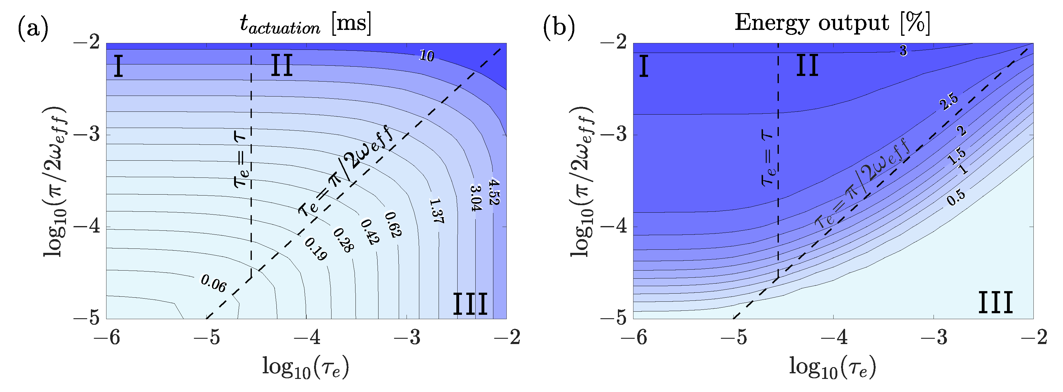
The previous section has shown that the performance of the actuated system strongly depends on the ratios between the heating time, ${\tau }_e$, and two important characteristics of the system, the mechanical response time of the system, $\pi /\left(2{\omega }_{eff}\right)$; and the kinetic response of the phase transformation, $\tau$. This leads to the identification of three different regimes:

• ${\tau }_e<\tau <\frac{\pi }{2{\omega }_{eff}}$; $t_{peakstress}\sim \tau$; $t_{actuation}\sim \frac{\pi }{2{\omega }_{eff}}$;
• $\tau <{\tau }_e<\frac{\pi }{2{\omega }_{eff}}$; $t_{peakstress}\sim {\tau }_e$; $t_{actuation}\sim \frac{\pi }{2{\omega }_{eff}}$;
• $\tau <\frac{\pi }{2{\omega }_{eff}}<{\tau }_e$; $t_{peakstress}\sim {\tau }_e$; $t_{actuation}\sim {\tau }_e$.

The actuator performance in the different regimes is demonstrated in Figure 19, which shows two main characteristics, actuation time (in units of ms) and energy output (percent), using contour lines which were generated by our computational model for a range of mechanical response time values, $\pi /2{\omega }_{eff}$. The two dashed lines in each panel are the regime boundaries, representing the cases in which the heating time equals either the characteristic transformation time, $\tau$ (in the vertical direction), or the mechanical response time, $\pi /2{\omega }_{eff}$ (with a slope of unity).

For a given ${\omega }_{eff}$, regime I is characterized by a high energy efficiency and a relatively short actuation time, $t_{actuation}$, determined by $\pi /2{\omega }_{eff}$. Notably, systems already placed in regime I, show almost no sensitivity to a shorter heating time, ${\tau }_e$, and so their desired performance can only be improved by increasing the value of ${\omega }_{eff}$, i.e., decreasing the mechanical response time, without a significant change in energy output. In regime II, the energy efficiency is slightly smaller, and the actuation time is slightly longer with respect to regime I. Regime III is characterized by a low energy efficiency, and long actuation times, $t_{actuation}$, determined by ${\tau }_e$.

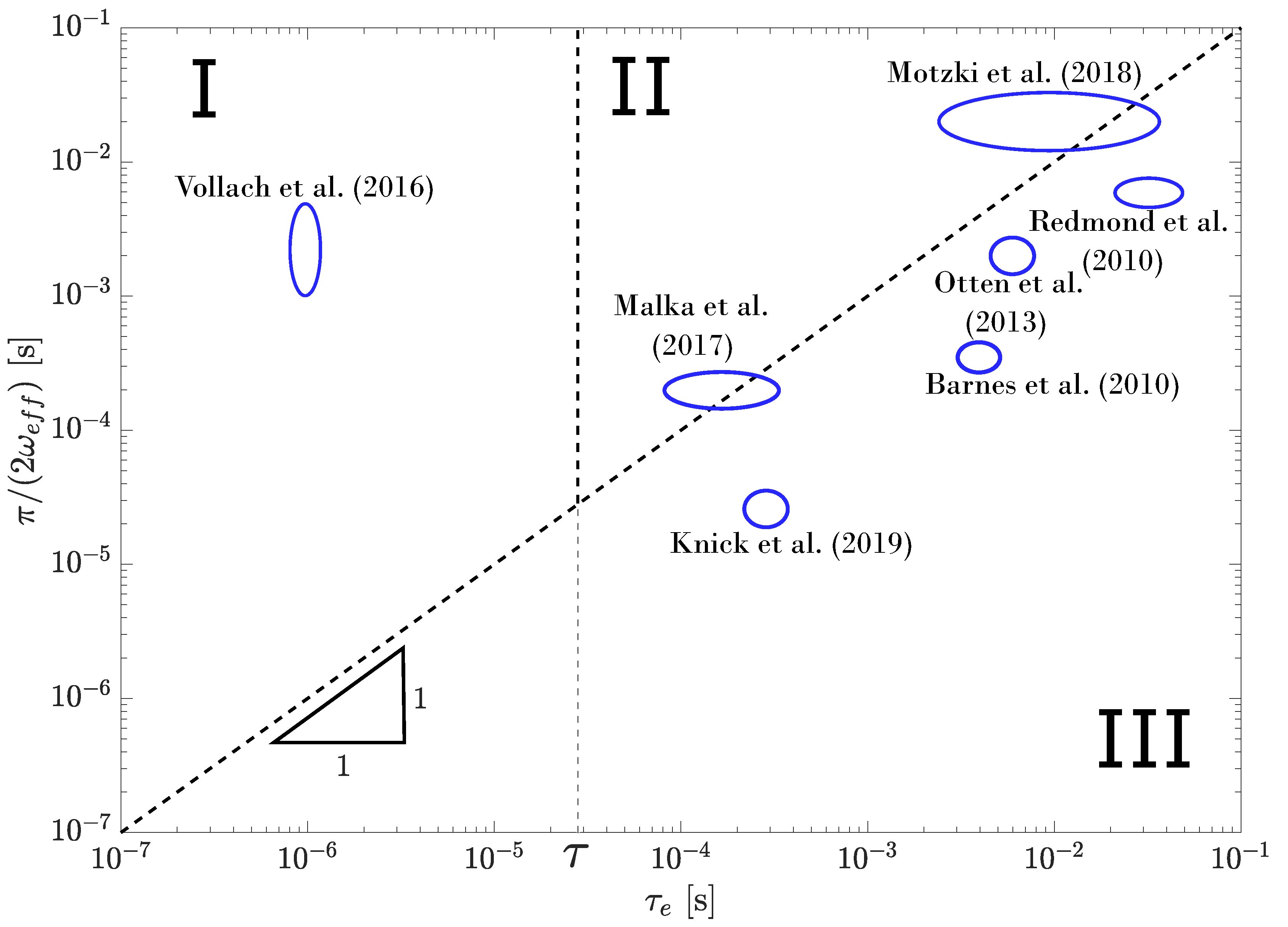
Figure 20 shows the respective location of a selection of previous experimental studies (Table 1) according to the three regimes. For example, Motzki et al. (2018) [36] obtained high energy efficiency using relatively low voltages (<125 V) but had to pay in a long actuation time (tens of ms, due to their low mechanical frequency) and time to peak stress (due to their slow heating rate, i.e., on the ms scale). Otten et al. (2013) [9] got shorter actuation times (compared to Motzki et al.) at relatively low voltages (<50 V), but had to pay in poor energy efficiency (due to their heating time being on the order of $\pi /2{\omega }_{eff}$). Vollach et al. (2016) [33] used very high voltages (2–4 kV), obtaining high energy efficiency and very short time to peak stress (tens on μs), but their actuation time was moderate (few ms, due to their low mechanical response rate). Malka et al. (2017) applied the smallest $\pi /2{\omega }_{eff}$ (for mm-scale systems) and moderate voltages (200–330 V) to obtain a heating rate, ${\tau }_e$, just slightly shorter than $\pi /2{\omega }_{eff}$. They got an energy efficiency that was just slightly lower than Vollach at al. and time to peak stress that was only slightly longer, but with a much shorter actuation time (by an order of magnitude).

All the aforementioned studies are examples for relatively large, mm-scale, actuators characterized by relatively large masses (with long mechanical response times) and large volumes of the SMA wire (affecting the required voltages for Joule-heating). At the same time, there is a recent growing interest in micro-scale actuator systems that are characterized by very small masses and small volumes of the SMA element [27,28,29,30,31,32]. Such systems have the potential to obtain very high energy efficiency values and short actuation times, if actuated using a fast electric pulse. Due to the small energy requirement, such short pulse duration can still be achieved using a low voltage. For example, Knick et al. (2019) used a MEMS bimorph actuator system based on a polymer layer (∼1 μm) with a thin layer (∼200 nm) of deposited NiTi. Their resulting mechanical response time of ∼25 μs is exceedingly small relative to the other systems, but their heating rate was much longer (0.3 ms). As a result, their actuator was operated in regime III and suffered from a poor energy efficiency. Nonetheless, a faster heating time of the small bimorph would quickly situate them in regimes I or II with an improved efficiency, along with a shorter time to peak stress and a shorter actuation time.

The unique characteristics of micro-scale systems, specifically their high mechanical response rate and low volume for heating make them prime candidates for high-rate actuation. Their low volumes typically result in a large resistance which allows for fast heating using low voltages, and they are typically able to provide relatively large forces with fast response rates in the μs-scale (e.g., References [27,28,29]).

10. Summary and Conclusions

This article reviews the different aspects of high-rate actuation of shape memory alloy wires in the high-driving-force regime.

The clamp-free configuration [9,21,24,33,35,36] is characteristic to actuator devices, where a mass or a mass-spring setup are attached at the free end. The governing equations are presented, and the effect of the natural mechanical frequency, ${\omega }_{eff}$, of the system is discussed. In particular, it was shown that, in a typical high-rate actuation, the characteristic time of the heating process should be much shorter than $\pi /2{\omega }_{eff}$.

An additional configuration (clamp-clamp), in which the wire was clamped at both ends [25,34,38,39], is used to study the intrinsic kinetics of the transformation. Under these boundary conditions, the transformation is unhindered by motion of masses or momentum transfer.

Section 1, Section 2 and Section 3 provided an introduction to the main aspects that have to be considered in the design of high-rate SMA actuators. These aspects include the required heating rate, applied force and the resulting energy input. High-rate actuation was also shown to result in excess kinetic energy following the end of the predefined actuator stroke, which can be utilised to increase the actuator travel-per-length. The basic insights introduced in these sections lead to rough design guidelines for the actuators and the selection of a suitable power source.

Section 4 and Section 5 presented detailed studies of the material behavior under high-rate conditions. Typical experimental results of both the clamp-free and clamp-clamp configurations have shown that their behavior within a time period of approximately $\pi /2{\omega }_{eff}$ from the onset of the heating pulse is similar, displaying a dead time followed by a rise in stress to a finite equilibrium stress plateau value, around which the stress oscillates due to string-like vibrations. At later times, behavior varies. The motion of the mass at the free end of the clamp-free configuration relieves the stress in the wire, allowing the volume fraction of the austenite phase to increase until the wire is fully at its austenite phase. The thermodynamic and kinetic rules presented in these sections are later used in the formulation of detailed model simulations.

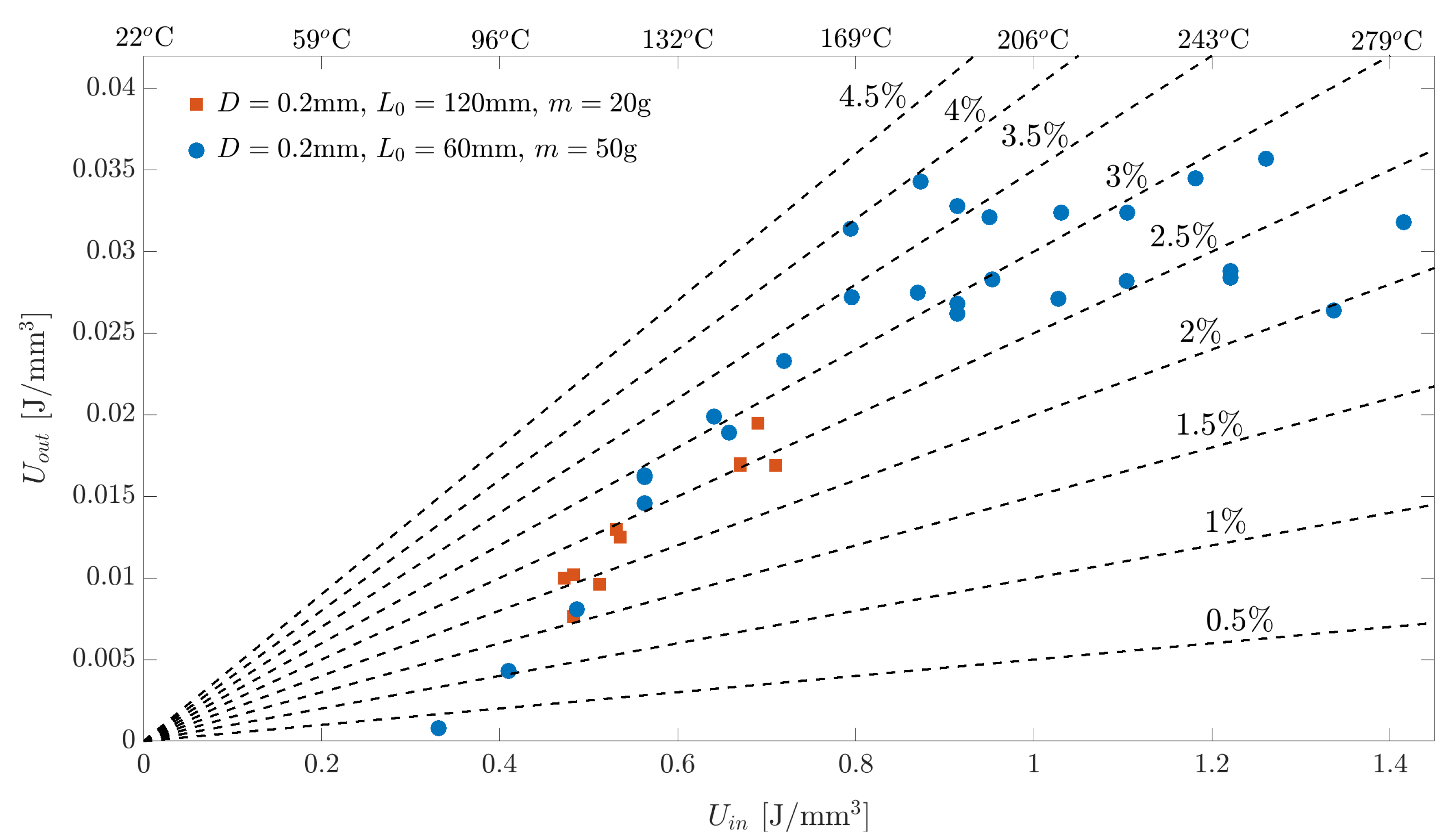
Section 6 presented phenomenological approximations of actuator performance, based on mappings the values of several key actuation characteristics under varying dimensions of the SMA wires and values of the actuated mass. Work outputs from a variety of experiments in the clamp-free configuration evaluated with respect to the specific input energy have shown that a large energy density provides an improved energy efficiency. Specifically, energy densities in the range 0.8–0.9 J/mm${}^3$ were shown to represent optimal operating conditions.

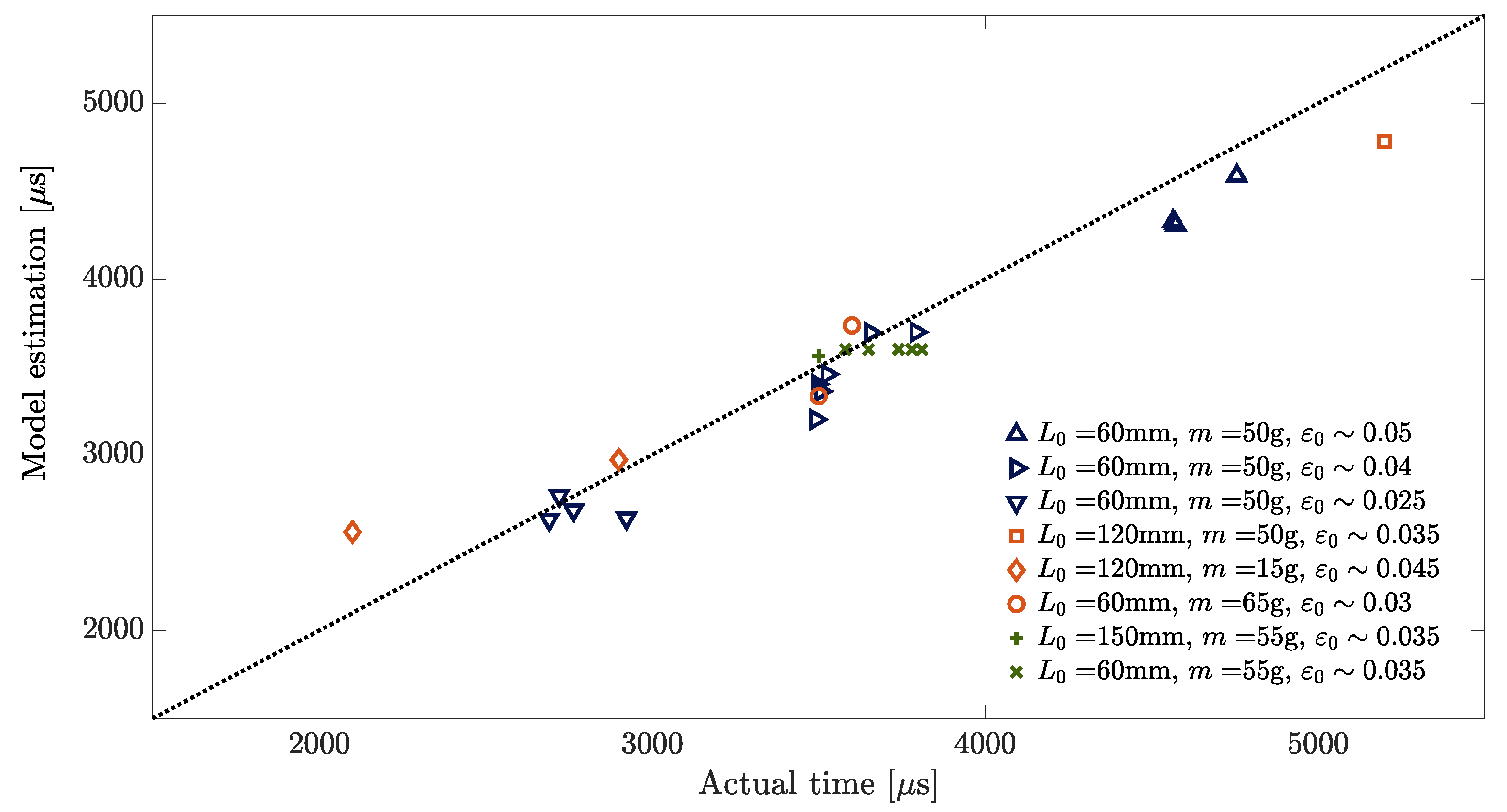
In Section 7, Section 8 and Section 9, we constructed and solved detailed simulations of actuator response that can serve as accurate design tools for specific applications. Model results were generated to simulate a clamp-free actuator with a freely hanging mass at its end. Two main cases were considered.

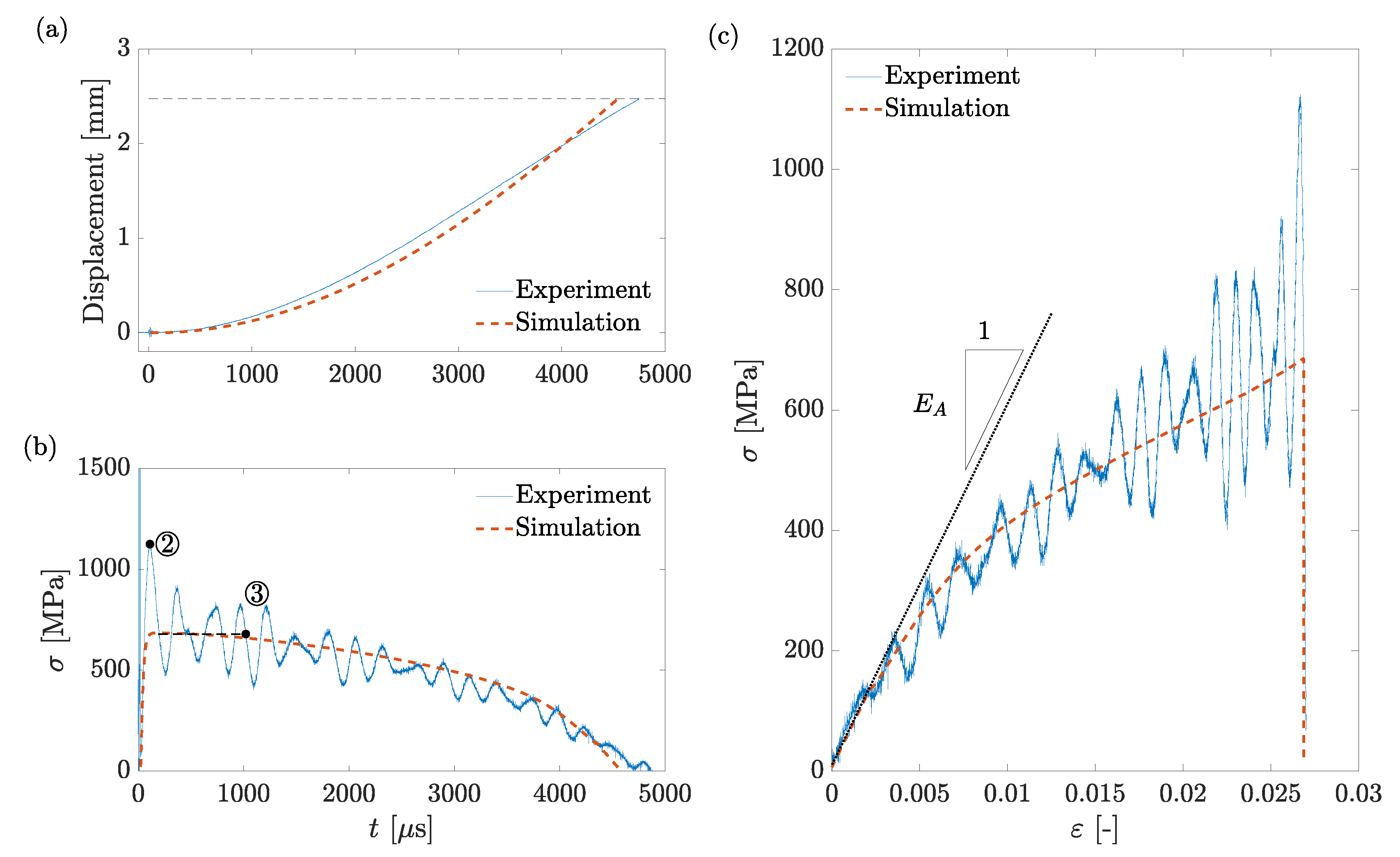
In the first case, the parameters of the simulation were taken to directly match those in the previously presented experiment of a typical clamp-free configuration. The compared simulated and experimental results have shown to be in striking correlation with each other, assuring the validity of the proposed model. This is a notably impressive feat owing to the extraction of all parameters from previous experimental data in both the clamp-free and clamp-clamp configuration and nullifying the need for empirical curve-fitting of specific parameters.

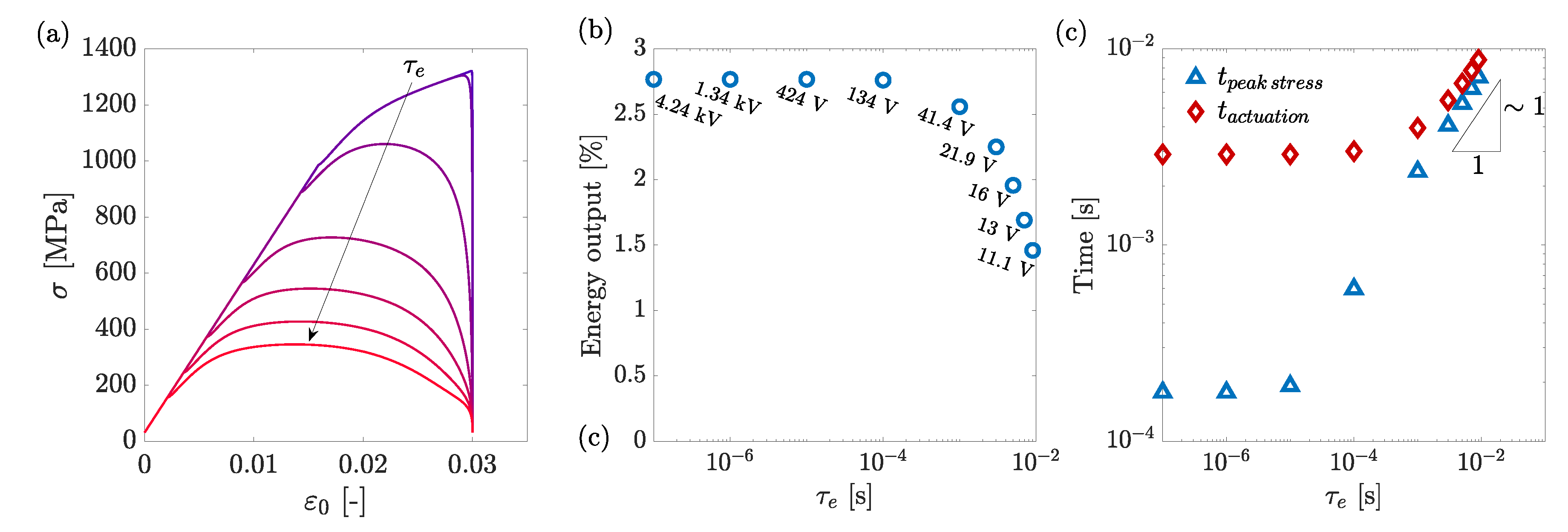
In a second case, we considered a wire of different dimensions under varying operating conditions and the effect of the characteristic pulse duration, ${\tau }_e$, was investigated. Characteristic heating durations up to the order of the characteristic response time of the phase transformation, $\tau$, (i.e., on the microsecond scale) were shown to produce larger work-per-volume output and increased energy efficiency, as well as shorter response times (to peak stress) and total actuation times. Notably, longer heating durations, in which the heating ended only after the transformation was complete, resulted in excess energy which was wasted on raising the temperature of the fully austenitic wire.

An important part in the design process of a high-rate SMA actuator involves the optimization of the required operating conditions. In particular, the application of a pulse heating power source was shown to impose a trade off between the use of low voltages (for improved safety and portability) and the resulting actuator performance, such as the actuation time and energy efficiency.

Finally, three different regimes of actuator performance were identified based on the applied heating rate and the mechanical response frequency of the system. These regimes enable users to quickly evaluate the expected performance of their system and consider the conditions that will secure an enhanced performance in terms of energy efficiency and actuation duration based on their needs.

References

1. Otsuka, K.; Wayman, C. Shape Memory Materials; Cambridge University Press: Cambridge, UK, 1999. [Google Scholar]
2. Bhattacharya, K. Microstructure of Martensite: Why It Forms and How It Gives Rise to the Shape-Memory Effect; Oxford University Press: Oxford, UK, 2003; Volume 2. [Google Scholar]
3. Ma, J.; Karaman, I.; Noebe, R. High temperature shape memory alloys. Int. Mater. Rev. 2010, 55, 257–315. [Google Scholar] [CrossRef]
4. Huber, J.; Fleck, N.; Ashby, M. The selection of mechanical actuators based on performance indices. Proc. R. Soc. Lond. Ser. A Math. Phys. Eng. Sci. 1997, 453, 2185–2205. [Google Scholar] [CrossRef]
5. Haghdoust, P.; Conte, A.L.; Cinquemani, S.; Lecis, N. Investigation of shape memory alloy embedded wind turbine blades for the passive control of vibrations. Smart Mater. Struct. 2018, 27, 105012. [Google Scholar] [CrossRef]
6. Lara-Quintanilla, A.; Hulskamp, A.W.; Bersee, H.E. A high-rate shape memory alloy actuator for aerodynamic load control on wind turbines. J. Intell. Mater. Syst. Struct. 2013, 24, 1834–1845. [Google Scholar] [CrossRef] [Green Version]
7. Karakalas, A.A.; Manolas, D.I.; Machairas, T.T.; Riziotis, V.A.; Saravanos, D.A. Active load alleviation potential of adaptive wind turbine blades using shape memory alloy actuators. Wind Energy 2019, 22, 620–637. [Google Scholar] [CrossRef]
8. Petrini, L.; Migliavacca, F. Biomedical applications of shape memory alloys. J. Metall. 2011, 2011, 501483. [Google Scholar] [CrossRef]
9. Otten, J.; Luntz, J.; Brei, D.; Strom, K.A.; Browne, A.L.; Johnson, N.L. Proof-of-concept of the shape memory alloy ReseTtable dual chamber lift device for pedestrian protection with tailorable performance. J. Mech. Des. 2013, 135, 061008. [Google Scholar] [CrossRef]
10. Hartl, D.J.; Lagoudas, D.C. Aerospace applications of shape memory alloys. Proc. Inst. Mech. Eng. Part G J. Aerosp. Eng. 2007, 221, 535–552. [Google Scholar] [CrossRef] [Green Version]
11. Copaci, D.; Blanco, D.; Moreno, L. Flexible Shape-Memory Alloy-Based Actuator: Mechanical Design Optimization According to Application. Actuators 2019, 8, 63. [Google Scholar] [CrossRef] [Green Version]
12. Britz, R.; Motzki, P.; Seelecke, S. Scalable Bi-Directional SMA-Based Rotational Actuator. Actuators 2019, 8, 60. [Google Scholar] [CrossRef] [Green Version]
13. Weirich, A.; Kuhlenkötter, B. Applicability of Shape Memory Alloys in Aircraft Interiors. Actuators 2019, 8, 61. [Google Scholar] [CrossRef] [Green Version]
14. Haigh, C.; Crews, J.; Wang, S.; Buckner, G. Multi-Objective Design Optimization of a Shape Memory Alloy Flexural Actuator. Actuators 2019, 8, 13. [Google Scholar] [CrossRef] [Green Version]
15. Yaguchi, H.; Kimura, I.; Sakuma, S. A Novel Actuator System Combining Mechanical Vibration and Magnetic Wheels Capable of Rotational Motion Using Shape Memory Alloy Coils. Actuators 2019, 8, 4. [Google Scholar] [CrossRef] [Green Version]
16. Ameduri, S.; Brindisi, A.; Ciminello, M.; Concilio, A.; Quaranta, V.; Brandizzi, M. Car Soundproof Improvement through an SMA Adaptive System. Actuators 2018, 7, 88. [Google Scholar] [CrossRef] [Green Version]
17. Lara-Quintanilla, A.; Bersee, H. A study on the contraction and cooling times of actively cooled shape memory alloy wires. J. Intell. Mater. Syst. Struct. 2016, 27, 403–417. [Google Scholar] [CrossRef]
18. Hartl, D.; Mingear, J.; Bielefeldt, B.; Rohmer, J.; Zamarripa, J.; Elwany, A. Towards high-frequency shape memory alloy actuators incorporating liquid metal energy circuits. Shape Mem. Superelasticity 2017, 3, 457–466. [Google Scholar] [CrossRef]
19. Barnes, B.; Brei, D.; Luntz, J.; Browne, A.; Strom, K. Panel deployment using ultrafast SMA latches. In Proceedings of the ASME International Mechanical Engineering Congress and Exposition, Chicago, IL, USA, 5–10 November 2006. [Google Scholar]
20. Barnes, B.M.; Brei, D.E.; Luntz, J.E.; Strom, K.; Browne, A.L.; Johnson, N. Shape memory alloy resetable spring lift for pedestrian protection. In Industrial and Commercial Applications of Smart Structures Technologies 2008; International Society for Optics and Photonics: Bellingham, WA, USA, 2008; Volume 6930, p. 693005. [Google Scholar]
21. Redmond, J.A.; Brei, D.; Luntz, J.; Browne, A.L.; Johnson, N.L.; Strom, K.A. The design and experimental validation of an ultrafast shape memory alloy resettable (smart) latch. J. Mech. Des. 2010, 132, 061007. [Google Scholar] [CrossRef] [Green Version]
22. Toma, M.; Luntz, J.; Brei, D.; Alexander, P.W.; Browne, A.L.; Johnson, N.L. Design and proof-of-concept validation of a latched arch active seal. J. Mech. Des. 2012, 134, 075001. [Google Scholar] [CrossRef]
23. Divi, S.; Ma, X.; Ilton, M.; St. Pierre, R.; Eslami, B.; Patek, S.; Bergbreiter, S. Latch-based control of energy output in spring actuated systems. J. R. Soc. Interface 2020, 17, 20200070. [Google Scholar] [CrossRef]
24. Malka, Y.; Shilo, D. A fast and powerful release mechanism based on pulse heating of shape memory wires. Smart Mater. Struct. 2017, 26, 095061. [Google Scholar] [CrossRef]
25. Mizrahi, A.; Heller, U.; Faran, E.; Shilo, D. Under-microscope mechanical pulse system for studying deformation processes at high strain rates. Exp. Mech. 2020, 60, 191–204. [Google Scholar] [CrossRef]
26. Mizrahi, A.; Shilo, D.; Faran, E. Variability of Twin Boundary Velocities in 10M Ni-Mn-Ga Measured Under μs-Scale Force Pulses. Shape Mem. Superelasticity 2020, 6, 45–53. [Google Scholar] [CrossRef]
27. Velez, C.; Kim, S.; Babaei, M.; Patel, D.K.; Knick, C.; Smith, G.; Bergbreiter, S. Rapid prototyping of microactuators by integrating 3D printed polymeric structures with NiTi thin film. In Proceedings of the 2020 IEEE 33rd International Conference on Micro Electro Mechanical Systems (MEMS), Vancouver, BC, Canada, 18–22 January 2020; pp. 893–896. [Google Scholar]
28. Velez, C.; Patel, D.K.; Kim, S.; Babaei, M.; Knick, C.R.; Smith, G.L.; Bergbreiter, S. Hierarchical Integration of Thin-Film NiTi Actuators Using Additive Manufacturing for Microrobotics. J. Microelectromech. Syst. 2020, 29, 867–873. [Google Scholar] [CrossRef]
29. Lee, H.T.; Kim, M.S.; Lee, G.Y.; Kim, C.S.; Ahn, S.H. Shape memory alloy (sma)-based microscale actuators with 60% deformation rate and 1.6 kHz actuation speed. Small 2018, 14, 1801023. [Google Scholar] [CrossRef] [PubMed]
30. Knick, C.R.; Sharar, D.J.; Wilson, A.A.; Smith, G.L.; Morris, C.J.; Bruck, H.A. High frequency, low power, electrically actuated shape memory alloy MEMS bimorph thermal actuators. J. Micromech. Microeng. 2019, 29, 075005. [Google Scholar] [CrossRef]
31. Liu, K.; Cheng, C.; Cheng, Z.; Wang, K.; Ramesh, R.; Wu, J. Giant-amplitude, high-work density microactuators with phase transition activated nanolayer bimorphs. Nano Lett. 2012, 12, 6302–6308. [Google Scholar] [CrossRef] [PubMed]
32. Babaei, M.; Kim, S.; Velez, C.; Patel, D.K.; Bergbreiter, S. Increasing the Energy Efficiency of NiTi Unimorph Actuators with a 3D-Printed Passive Layer. J. Microelectromech. Syst. 2020, 29, 797–803. [Google Scholar] [CrossRef]
33. Vollach, S.; Shilo, D.; Shlagman, H. Mechanical response of shape memory alloys under a rapid heating pulse-part II. Exp. Mech. 2016, 56, 1465–1475. [Google Scholar] [CrossRef]
34. Dana, A.; Sekiguchi, H.; Aoyama, K.; Faran, E.; Liss, K.D.; Shilo, D. The evolution of the martensitic transformation at the high-driving-force regime: A microsecond-scale time-resolved X-ray diffraction study. J. Alloys Compd. 2021, 856, 157968. [Google Scholar] [CrossRef]
35. Volkov, A.E.; Miszuris, W.; Volkova, N.A. Strain Recovery by TiNi Element Under Fast Heating. Shape Mem. Superelasticity 2018, 4, 256–263. [Google Scholar] [CrossRef]
36. Motzki, P.; Gorges, T.; Kappel, M.; Schmidt, M.; Rizzello, G.; Seelecke, S. High-speed and high-efficiency shape memory alloy actuation. Smart Mater. Struct. 2018, 27, 075047. [Google Scholar] [CrossRef]
37. Casati, R.; Passaretti, F.; Tuissi, A. Effect of electrical heating conditions on functional fatigue of thin NiTi wire for shape memory actuators. Procedia Eng. 2011, 10, 3423–3428. [Google Scholar] [CrossRef]
38. Vollach, S.; Shlagman, H.; Shilo, D. Kinetics of the reverse martensitic transformation in shape memory alloys under an abrupt heating pulse. Scr. Mater. 2017, 135, 76–79. [Google Scholar] [CrossRef]
39. Vollach, S.; Caciularu, R.; Shilo, D. Equilibrium stress during the response of shape memory alloys to an abrupt heat pulse. Scr. Mater. 2017, 141, 50–53. [Google Scholar] [CrossRef]
40. Vollach, S.; Shilo, D. The mechanical response of shape memory alloys under a rapid heating pulse. Exp. Mech. 2010, 50, 803–811. [Google Scholar] [CrossRef]
41. Dynalloy, I. Technical characteristics of flexinol actuator wires. CA Tustin 2011, 690. [Google Scholar]
42. Bekefi, G.; Barrett, A.H. Electromagnetic Vibrations, Waves, and Radiation; MIT Press: Cambridge, MA, USA, 1977. [Google Scholar]
43. Churchill, C.; Shaw, J. Behavior and mechanics of multifunctional and composite materials. In Proceedings of the SPIE, Marseille, France, 23–28 June 2008. [Google Scholar]
44. Troisfontaine, N.; Bidaud, P.; Larnicol, M. Optimal design of micro-actuators based on SMA wires. Smart Mater. Struct. 1999, 8, 197. [Google Scholar] [CrossRef]
45. Thomasová, M.; Sedlák, P.; Seiner, H.; Janovská, M.; Kabla, M.; Shilo, D.; Landa, M. Young’s moduli of sputter-deposited NiTi films determined by resonant ultrasound spectroscopy: Austenite, R-phase, and martensite. Scr. Mater. 2015, 101, 24–27. [Google Scholar] [CrossRef]
46. Dana, A.; Sekiguchi, H.; Aoyama, K.; Faran, E.; Liss, K.D.; Shilo, D. Dynamics of Phase Fronts During High-Driving-Force Transformation of Shape Memory Alloy Wires. Shape Mem. Superelasticity 2021, 1–11. [Google Scholar] [CrossRef]
47. Reedlunn, B.; Daly, S.; Hector, L.; Zavattieri, P.; Shaw, J. Tips and tricks for characterizing shape memory wire part 5: Full-field strain measurement by digital image correlation. Exp. Tech. 2013, 37, 62–78. [Google Scholar] [CrossRef] [Green Version]
48. Šittner, P.; Sedlák, P.; Seiner, H.; Sedmák, P.; Pilch, J.; Delville, R.; Heller, L.; Kadeřávek, L. On the coupling between martensitic transformation and plasticity in NiTi: Experiments and continuum based modelling. Prog. Mater. Sci. 2018, 98, 249–298. [Google Scholar] [CrossRef]
49. Vollach, S. The Mechanical Response and Phase Transformation Kinetics of NiTi under a Rapid Heating Pulse. Ph.D. Thesis, Department of Mechanical Engineering, Technion—Israel Institute of Technology, Haifa, Israel, 2018. [Google Scholar]
50. Heller, L.; Seiner, H.; Šittner, P.; Sedlák, P.; Tyc, O.; Kadeřávek, L. On the plastic deformation accompanying cyclic martensitic transformation in thermomechanically loaded NiTi. Int. J. Plast. 2018, 111, 53–71. [Google Scholar] [CrossRef]
51. Chen, Y.; Molnárová, O.; Tyc, O.; Kadeřávek, L.; Heller, L.; Šittner, P. Recoverability of large strains and deformation twinning in martensite during tensile deformation of NiTi shape memory alloy polycrystals. Acta Mater. 2019, 180, 243–259. [Google Scholar] [CrossRef]
Figure 1. Schematics of a conceptual tablecloth-trick latch mechanism, based on fast SMA actuation, designed to reduce the required work output. The friction force at the contact between the deployed structure (large mass), M, and the latch (small mass), m, is greatly reduced by disengaging the masses as result of rapid actuation, compared with slow release [24].
Actuators 10 00140 g001
Figure 2. Schematics of an SMA actuator in a spring-mass configuration. (a) The SMA wire is connected to a mass and spring at its free-end. In ①, the wire is completely in its detwinned martensitic phase with a strain of ε 0 relative to its original length in the austenite phase. In ②, the wire is completely in its austenite phase with an elastic strain of ε e l A . (b) Diagram of austenite-martensite transformations in the stress-strain space. The upper flag diagram (thin solid lines) is the superelastic transformation path at temperatures above A f . The lower curve (bold solid line) is the detwinning path at temperatures below M f , Points ① and ② correspond with the diagrams in (a). The dashed lines denoted by σ Q S ( ε ) and σ D y n ( ε ) are the shape-memory transformation paths under quasi-steady and rapid heating, respectively.
Actuators 10 00140 g002
Figure 3. Schematics of the mechanical set-ups of the two experimental configurations: (a) clamp-free; (b) clamp-clamp.
Actuators 10 00140 g003
Figure 4. Typical results of experiments in the clamp-free configuration of NiTi wires. The wire diameter was 0.38 mm and its length 93 mm, its free end was attached to a mass large enough to keep it aligned prior to actuation. (a) Heating pulse of electric power transferred to the wire. (A zoomed-in view of the shape of the electric pulse is presented in the top panel of Figure 6.) (b) Displacement measurements taken at the bottom end of the mass. (c) Stress evolution in the wire. Points ①–④ signify the dead time of the wire, peak stress, onset of stress decrease in the wire, and the end of the transformation, respectively. The dashed line represents the equilibrium stress averaged over the first 1000 μs. (d) Stress-strain curve plotted based on the data from figures (b,c). Points ③ and ④ are the same as in (c). The linear dotted line has a slope equal to the elastic modulus of austenite, E A , signifying the elastic relaxation of the austenitic wire at the end of the transformation.
Actuators 10 00140 g004
Figure 5. Typical macroscopic stress results from experiments in the clamp-clamp configuration. The onset of the electric pulse was chosen as t = 0 . The curves show the measured tensile stress, in units of MPa, at each end of the SMA wire over a 4 ms time-period. The inset shows a zoom-in into the initial 100 μs.
Actuators 10 00140 g005
Figure 6. Typical results of experiments in the clamp-clamp configuration. (Top) Average wire temperature evolution in time, based on Ref. [34]. The dotted line shows the ∼3 μs pulse of electric power transferred to the wire, in normalized units, the onset of the electric pulse was chosen as t = 0 . (Bottom) The blue squares are the integrated XRD intensity I A ( t ) of the austenite 110 A peak, normalized with respect to its mean final value (i.e., mean of plateau after 20 μs), corresponding to an estimated austenite volume fraction of 0.261 [46]. The solid curve is the mean measured tensile stress from all experiments shown in units of MPa, marked on the right vertical axis. The horizontal dashed line represents the equilibrium stress value averaged over the interval [1.4, 5] ms after the pulse (See Figure 5). The vertical dashed lines denote the different stages of the transformation. Reproduced from Dana et al. (2021) [34] with permission from Elsevier.
Actuators 10 00140 g006
Figure 7. Effect of temperature on typical experiments in the clamp-clamp configuration. The wire temperatures immediately after the pulse are in the range T [ 100 , 120 , 142 , 168 , 195 , 209 ] . (a) Zoom-in on the beginning of stress versus time curves measured by one of the force sensors, using the same wire and same initial stress, under different input energies. (b) Normalized stress profiles (the left hand side of Equation (17)) for the curves presented in (a). (c) The stress versus time curves in (a) presented over a larger period in the millisecond scale, showing the change in equilibrium stress.
Actuators 10 00140 g007
Figure 8. Equilibrium stress, σ e q (left axis), as a function of temperature for experiments performed on a wire with a diameter of 0.2 mm and a length of 48 mm (the same as shown in Figure 7). In all tests, the initial stress was set to σ 0 = 200 MPa. The corresponding austenite volume fraction, x e q (right axis), for each point, was calculated using Equation (15).
Actuators 10 00140 g008
Figure 9. Transition temperature as a function of the austenite volume fraction, measured at equilibrium under a constant stress of 20 MPa. The curved lines represent a fit to Equation (20a,b) with T 1 = 24 C, T 2 = 72 C, T 3 = 71 C, T 4 = 88 C, λ 1 = 0.073 and λ 2 = 0.03 .
Actuators 10 00140 g009
Figure 10. Measurements of the equilibrium stress, σ e q , under different applied initial stress values, σ 0 . The dashed lines represent calculations of σ e q as a function of σ 0 for constant T values, as indicated near each line.
Actuators 10 00140 g010
Figure 11. Energy efficiency of a clamp-free actuator. Mechanical work output, U o u t , presented as a function of the electrical input energy, U i n , based on Equation (3). The dashed lines represent different energy efficiencies based on the ratio between the specific output and input energies.
Actuators 10 00140 g011
Figure 12. Approximated linear model for the stress-strain profile of the clamp-free experiment presented in Figure 4.
Actuators 10 00140 g012
Figure 13. Duration of Actuation—predictive model versus actual tests. Data was taken from experiments reported in Refs. [33,49].
Actuators 10 00140 g013
Figure 14. (a) Evolution of the stress profile over 20 consecutive rapid heating actuations. (b) Strain recovery under slow-rate heating in a thermal bath as a function of the temperature following the corresponding actuation cycle in (a). The dotted line represents a virgin wire that was never actuated prior to the heating test.
Actuators 10 00140 g014
Figure 15. Results of a simulation of our typical experiment presented in Figure 4. (a,b) The time evolution of the energy input into the wire normalized by its maximum value; U i n ( t ) / U 0 , is presented in the blue dashed curve, and the evolution of the volume fraction of austenite, x ( t ) , in the solid red curve. (c,d) The temperature evolution of the wire in time, T ( t ) , is presented in the red solid curve, and the evolution of the volume-fraction-dependant transition temperature, T ˜ ( x ) , in the blue dashed curve. (a,c) A zoom-in into the initial 100 μs after the onset of the heating pulse.
Actuators 10 00140 g015
Figure 16. Comparison of experimental results with our simulation. (a) Time evolution of the measured and simulated displacement. The horizontal thin dashed line represents the maximal displacement of the wire due to the original strain of the detwinned martensite phase. (b) Stress evolution in time. The experimental solid curve oscillates around the simulated curve. (c) Stress-strain curves of both the experimental measurements and simulated results. The linear dotted line signifies the elastic relaxation of the austenitic wire with slope E A , corresponding to its elastic modulus.
Actuators 10 00140 g016
Figure 17. Simulated results of NiTi wire actuation at different values of characteristic heating time, τ e [ 10 6 , 10 4 , 10 3 ] s. Calculations considered a wire with diameter d = 0.2 mm and length L 0 = 50 mm subjected to an initial strain of ε 0 = 0.03 , an attached mass of 0.1 kg, and a discharged energy density U 0 = 0.9 J/mm 3 . (a,b) Stress evolution in time, σ ( t ) . (c,d) Normalized discharged energy onto the wire, U i n ( t ) / U 0 . (e,f) Austenite volume fraction, x ( t ) . (g,h) Wire temperature evolution in time, T ( t ) . (a,c,e,g) A zoom-in into the initial 200 μs after the onset of the heating pulse. The heating time, τ e , increases in the direction of the annotated arrows.
Actuators 10 00140 g017
Figure 18. Actuation performance of a NiTi wire at different values of τ e . The simulated configuration corresponds to that presented in Figure 17. (a) Stress evolution as a function of strain. (b) Energy output of the actuation cycle for different values of τ e . The output energy was normalized relative to the energy fraction invested in the phase transformation, U i n ( x = 1 ) . A corresponding actuation voltage for each value of τ e was calculated based on Equations (9) and (10). (c) Actuation duration, t a c t u a t i o n , and response time, t p e a k s t r e s s , for different values of τ e .
Actuators 10 00140 g018
Figure 19. Contour plots of key measures for actuator performance as a function of the heating time, τ e , and the mechanical response time, π / 2 ω e f f . (a) Total actuation time, t a c t u a t i o n , in ms. (b) Energy output (percent), calculated relative to the invested energy for heating up to x = 1 . The dashed lines represent boundaries of the different regimes denoted by I, II, and III. In (a), lower values (brighter colors) are preferred, while, in (b), larger values (darker colors) are preferred.
Actuators 10 00140 g019
Figure 20. Comparison of previous experimental studies based on the different actuation regimes (see Figure 19).
Actuators 10 00140 g020