An Adaptive Model Predictive Control System for Virtual Coupling in Metros

Abstract

Virtual coupling (VC) is an emerging concept and hot research topic in railways, especially for metro systems. Several unit trains in VC drive with a desired minimum distance, and they, as a whole, are regarded as a single train. In this work, a distributed adaptive model predictive control (AMPC) system is proposed to coordinate the driving of each unit train in VC. To obtain the accurate parameters of train dynamics model in a time varying environment, an estimator of the train dynamics model is designed for each AMPC controller. A variable step descent algorithm along the negative gradient direction is adopted for each estimator, which steers the estimated values of the parameters to real ones. Simulations are conducted and the results are compared with both nominal model predictive control system and AMPC system with fixed steps in the literature. Our proposed AMPC system with variable step (AMPCVS) has better performances than other two systems. Results indicate that there is an improvement of the proposed AMPC system with variable steps system when compared with other two existed systems. A running process of VC in a whole inter-station is also simulated here. Experimental results show that the trains track the desired objective well.

1. Introduction

Metro transportation is favored by people as a public transportation. The increasingly population in cities raises the requirement to enhance the track capacity of metro. The track capacity is determined by the amount of tracks and the performance of operation system. It is unrealistic to build as much track we can, which costs a lot in manpower and material resources. Therefore, there exists an expectation to design a novel operation system that increases the track capacity. Nowadays, there is a manual process for trains to couple together by couplers. This process helps adjacent trains keep a minimum distance. However, for the trains which are not coupled by the coupler, they are supposed to be separated by a much greater distance. It wastes a certain amount of track capacity. Virtual coupling (VC) is a system, in the future, towards train operation. It is proposed to reduce the distance between adjacent trains which are not coupled by the coupler but have same route ahead [1]. This concept increases the track capacity by making individual trains separated closer, and saves preparing time by cancelling the manual coupling process. So, VC is a potential and sensible choice to enhance the track capacity, by these advantages.

VC was first proposed in 1999 which aims at making railway freight transportation more attractive than road transportation [2]. The authors thought the best solution to increase track capacity is to have long trains on long and branchless railroads, and to split them into smaller parts before a junction [3]. Therefore, the trains should not be physically coupled, which cannot be split during driving. Additionally, each train should have its own propulsion and control system to support the automatic driving. Inspired by this, much research was conducted which further polished the definition of VC. Konig et al. [4] reckon that trains are separated by the distance much less than the absolute (and even relative) braking distance, though these two represent the state-of-the-art. Due to the immaturity of other technical conditions at that time, the potential of VC could not be truly realized [5]. Based on the improvement of communication technology, Flammini et al. [6] adopt a train-to-train communication, which exists besides the train-to-track communication. Such that, all connected trains are able to share real-time information with neighbors and to receive the reference signals coming from the infrastructure. The utilization of real-time information brings huge potential for the train operation in VC. Henke et al. [7] raise that trains in VC should be autonomous and travel on demand instead of operating on a fixed schedule. Another conception from Goikoetxea [8] is that each train in convoy should be commanded by a leader train. To make the trains in VC analogously physically coupled, Quaglietta et al. [1] propose that the trains should move synchronously in a convoy and can be treated as a single train at junctions in the view of schedule.

VC may be applied to the metro first [9]. Compared with high-speed and regional, trains in metro will not suffer some severe weather and drive at a relatively fixed speed. These decrease the difficulty of train control. Another biggest characteristic of metro is the tidal passenger flow. VC can flexibly adjust the length of trains to meet the amount of tidal passengers. Additionally, the localization and measurement are more accurate in metro because of the short travelling distance in the inter-station. Therefore, we consider chose the metro as our application objective.

One of the indicators of VC performances is the distance between adjacent trains. The distance is mainly determined by a protection method. The general idea of protection is making a regulation for trains. Normally, the regulation is to set a protection distance between trains. Once the distance between trains becomes smaller than protection, the train must brake to standstill urgently and irrevocably. One method is to make trains separated by a constant distance, imitating the physically coupled condition. Physically coupled trains are connected by a coupler whose length is an approximately fixed value. Some research present control systems which keep a constant distance [1,10,11,12]. The faster trains are, the more likely they will collide, resulting from errors or faults. Thus, a kilometric scale distance was used to keep safe for high-speed trains, achieving cooperative driving under moving-block mode in [11,12]. However, [1,10] focus on the metro that trains drive at a lower speed so that the distance is set as 10 m. Trains separated by a constant distance can realize moving synchronously, i.e., moving at a same speed. Therefore, the constant distance will be ultimately necessary, although it seems immaturity now.

If there were neither uncertainty disturbances, nor delay or packet loss in communication [13], or nor localization and measurement errors, the desired distance can be set as a minimum fixed value in VC. Therefore, the localization and communication technologies are significant to VC, which also determine how well the performance of VC is. The localization can be realized by ground equipment (e.g., balise), onboard equipment (e.g., GNSS-based [14,15]), or both. With the development of modern technology, such as GSM-R, DSRC [16], and 5G, it is possible to share and receive the information of position, velocity, acceleration and even future driving route. 5G is used by neighbor trains to obtain a low time-delay and high quality communication [17].

Then, with the accurate information of other trains and a safe protection method, it is supposed to design an efficient and stable train control system to keep the desired distance between trains. In recent publications about VC, feedback control [1], model predictive control (MPC) [10], multi-agent system (MAS) control [18] and sliding mode control (SMC) [19] are used to realize train automatic drive. The feedback control and MAS control need to be carefully designed since the existing limitations with respect to the track condition and train property. SMC tracks the reference accurately but cannot respond ahead of time to the future action of predecessor train. The MPC in [10] adopts a nominal model of train regardless of parameters errors. Thus, we proposed an adaptive model predictive control (AMPC) algorithm in this paper with an estimator that makes the model of plant more accurate.

MPC is a form of control in which the current control action is obtained by solving online, at each sampling instant, a finite horizon open-loop optimal control problem, using the current state of the plant as the initial state [20]. To fully utilize the value of real-time information, only the first one of control input sequence, i.e., the solution of the optimal control problem above, is applied to the plant. At next sampling instant, the process above is repeated. MPC can actively deal with constraints in the control problem and then avoids some hazard condition. The optimal control problem has a finite prediction horizon so that the resultant controller does not guarantee the stability mathematically. Stability is achieved in most process applications since the horizon of the optimal control problem is normally sufficiently long [21]. A method to guarantee the stability of MPC system mathematically is to extend the prediction horizon to a quasi-infinite prediction horizon by adding a terminal cost function and terminal constraint [20]. Then, the nominal MPC, which is based on a known and accurate model of plant, performs well in this way. However, there actually exist some uncertain elements between the nominal model in MPC and the real model. The uncertain elements result in the errors of system from desired states. The system will become uncontrollable and unstable since the constraints are broken by accumulated errors. Robust MPC (RMPC) is designed for the purpose of this situation. A traditional RMPC method uses a Min–Max principle to design a controller input which is robust to the worst condition [22]. Another approach, named tube-based MPC [23,24], controls the real system by keeping it in the tube set [25]. These two methods protect the constraints from the broken. However, if the model of plant is accurate enough, the error of state will be eliminated fundamentally. So, Zhu et al [26] present an adaptive model predictive control (AMPC) algorithm which makes the estimated model approach to the real model step by step. It is proved that the estimated model is bounded and the system state will converge to a neighborhood around an equilibrium point. This algorithm is used into several fields, like spacecraft [27] and high-speed trains [28]. However, this algorithm requires the error of state to satisfy a fixed constraint all the time which has been set before the initialization.

Based on the previous research, we present a distributed AMPC system, which does not have any more requirements to bound the error of system, to realize the desired train control, keeping a desired distance between adjacent trains. Our main contributions are as follows:

• A serial distributed control system structure is proposed for trains in VC, according to the metro infrastructures and their communication architectures, where each train has a local controller and each controller communicates with its neighbor trains. Based on the control structure, a distributed AMPC system is proposed to make successive trains driving with a desired distance;
• An estimator is designed for each local controller in the distributed AMPC system, to reduce the value errors between parameters in the model and real ones. A variable step gradient descent method is proposed which guarantees the estimated model is bounded;
• Simulations are conducted, and the proposed AMPC with a variable step (AMPCVS) system is compared with both nominal MPC system and AMPC with a fixed step (AMPCFS) system. Experimental results prove that the distance error between the actual and desired ones for successive trains in AMPCVS is much smaller than nominal MPC system, and the error in AMPCVS approximates zero faster than the AMPCFS system. These indicate that there is surely an improvement of AMPCVS algorithm when compared to other two systems.

The rest of this paper is organized as follows. In Section 2, a train dynamics model is formulated, and a serial distributed control system structure for trains in VC is proposed. A distributed AMPC system is designed in Section 3, where the control model for both leader and following trains are formulated, and an estimator is designed for each local controller to make the system model adapt to time varying environments. Experimental results are presented in Section 4, which show that trains in VC keep the desired distance well by using our proposed algorithm. Finally, Section 5 concludes this paper.

2. Train Dynamics and Virtual Coupling Strategy

2.1. Train Dynamics Model

Based on the longitudinal train dynamics, the dynamic model of train is written as

$$\left\{\begin{array}{c}\dot{p}=v\hfill \\ \dot{v}=-c_0-c_{1}v-c_2{v}^2+F/m\hfill \\ \dot{F}/m=(u-F)/\left(mT\right)\hfill \end{array}\right.$$

(1)

where p, v and F represent the position, velocity and applied force of the train, respectively. m is the mass of train. $c_0$, $c_1$ and $c_2$ are the constant parameters of the Davies equation which represents the aerodynamic resistance force. They will vary with respect to the different condition so that the values in model are estimated by human experience. The control variable u denotes the control input force. The dynamic characteristic of train actuator is simplified as an inertial element. However, the time constant T is also estimated by human experience which is not accurate. Thus, the train dynamic model that we can establish is just an estimated model which is written as

$$\left\{\begin{array}{c}\dot{p}=v\hfill \\ \dot{v}=-{\widehat{c}}_0-{\widehat{c}}_{1}v-{\widehat{c}}_2{v}^2+F/m\hfill \\ \dot{F}/m=(u-F)/\left(m\widehat{T}\right)\hfill \end{array}\right.$$

(2)

where $\widehat{(·)}$ represents the estimated value of the parameter $(·)$ in (1).

All trains in VC is limited with respect to the performance of train and track. Due to the property limitation of train itself, the controlled input force is bounded as

$$u_{min}\le u\le u_{max}$$

(3)

where $u_{min}$ denotes the maximum reverse force and $u_{max}$ denotes the maximum positive force. The trains is also limited by a hard constraint in speed as

$$0\le v\le v_{lim}$$

(4)

where $v_{lim}$ is the track speed limitation with respect to the track condition.

As we mentioned above, trains in VC are supposed to move together and to be separated by a constant distance. Thus, the protection distance should be set as a constant value so that trains are protected from collisions by

$$\begin{array}{cc}{p}_{i-1}-L-p_i\ge d_e,& i=2,3,\cdots \end{array}$$

(5)

where $d_e$ is the protection distance and L denotes the length of train. For avoiding braking to standstill frequently, the protection distance should be smaller than the desired distance $d_r$ as $d_e\le d_r$. It is worthwhile to notice that this constraint is only for the followers. As the traditional method in railways, there is a speed limitation for the leader to guarantee keeping a safe distance from the hazard ahead. For simplicity, we assume that the speed limitation for the leader is included in the constraint (4).

2.2. Control Structure of Trains in VC

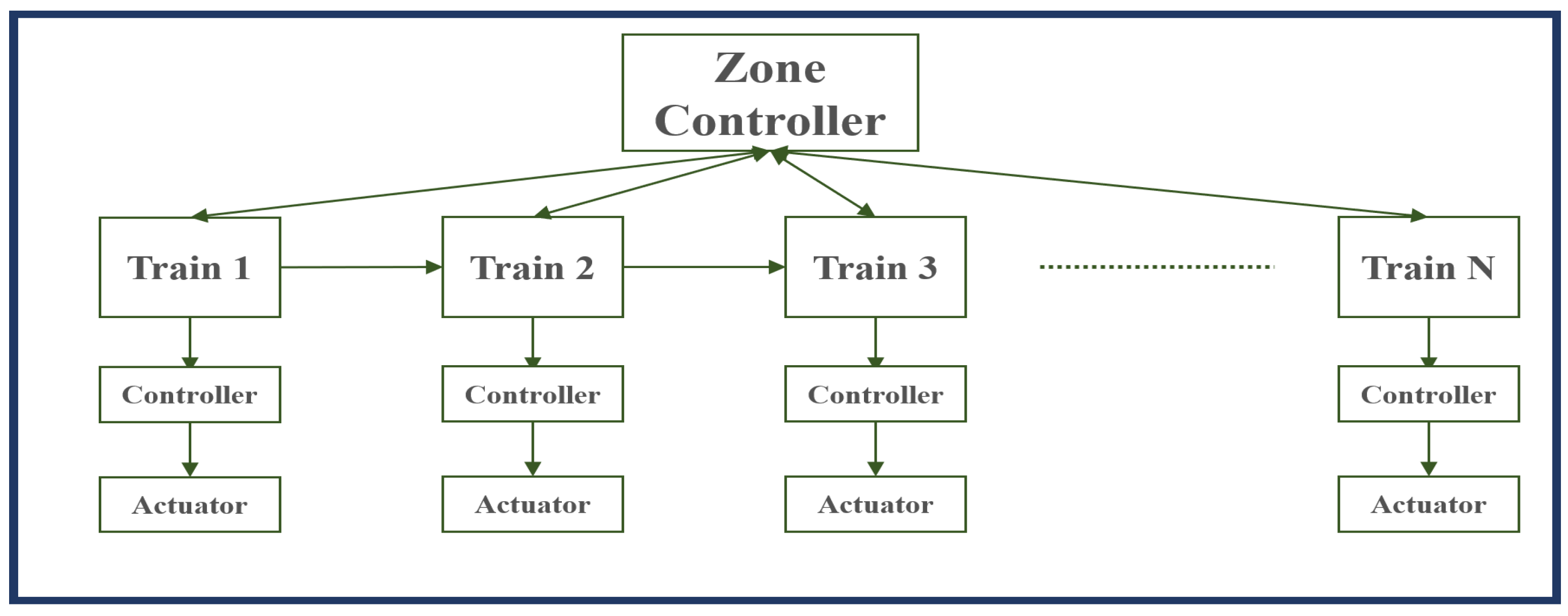
The trains in VC are connected via T2T and T2G communication instead of couplers. Through the link between trains, each train is able to receive the control objective from a global controller and the required information from other trains, as shown in Figure 1. This communication topology provides the convenience to the distributed control system. Then, the distributed control structure shown in Figure 2 is realized. It implies that the controller for each train in VC can be different and all of them are managed by the zone controller (ZC).

As for a physically coupled train, the objective is tracking a desired speed profile. Those wagons, without independent propulsion units, are applied force by couplers to keep an approximate constant distance from its predecessor wagon. It avoids beyond the extreme displacement of coupler and results in tracking the desired speed. In VC, trains are supposed to move together just like physically coupled, which means the driving strategies for the leader and the followers in VC are different. The leader should track the desired speed profile and the followers should keep a desired distance from their predecessors.

There does not exist any predecessor train for the leader train, just like the first wagon in a physically coupled train. The objective of the first wagon train is tracking the desired speed. Therefore, the driving strategy for the leader is driving at the desired speed to manage the speed of convoy. The control objective is written as

$$v_1=v_r$$

(6)

where subscript 1 means the state of train 1 and $v_r$ denotes the desired speed.

Each wagon in a physically coupled train is supposed to maintain a constant distance to its predecessor to keep the integrity. To imitate the state of physically coupled train, the driving strategy for the followers is to keep a constant distance which is called as the desired distance. Then, the control objective becomes

$$p_{i-1}-L-p_i=d_r$$

(7)

where $d_r$ is the desired distance for adjacent trains in VC.

With respect to the different control objectives for the leader and followers, different controllers are presented in Section 3 and the states of control system are correspondingly different.

Based on the control objective above, ZC delivers the control objective to each train. Each controller calculates a proper control input for an actuator. The actuator applies actions to the train to adjust its system state. Then, the dynamic information (e.g., position, speed, applied force) of each train will be sent back to ZC. Then, ZC refreshes and generates a new objective for the leader train. Meanwhile, the dynamic information will be sent, from the predecessor, to the follower so that the controller of follower can calculate the control input to keep a desired distance from the predecessor. The distributed structure has been described briefly here, which will be designed in details, in Section 3.2.

3. Distributed Adaptive Model Predictive Control System Designs

3.1. Control System Model

The control objective of leader is to track a desired speed profile. Therefore, the state of control system for the leader is chosen as

$$x_1={[{\tilde{p}}_1,{\tilde{v}}_1,F_1]}^T$$

(8)

where ${\tilde{p}}_1=p_1-p_r$ and ${\tilde{v}}_1=v_1-v_r$. $p_r$ is the desired position. For the follower train i ($i=2,3,\cdots$) in VC, corresponding to the control objective that keeps a desired distance from predecessor, the state is chosen as

$$x_i={[{\tilde{p}}_i,{\tilde{v}}_i,F_i]}^T$$

(9)

where ${\tilde{p}}_i=p_i+L+d_r-p_{i-1}$, ${\tilde{v}}_i=v_i-v_{i-1}$. Then, the linearized continuous model of N trains based on (2) (8) (9) is written as

$$\left\{\begin{array}{c}{\dot{\tilde{p}}}_i={\tilde{v}}_i,i=1,2,\cdots ,N\hfill \\ {\dot{\tilde{v}}}_1=-{\widehat{c}}_1{\tilde{v}}_1-{\widehat{c}}_2{v}_r{\tilde{v}}_1+F_1/m-{\widehat{c}}_0\hfill \\ {\dot{\tilde{v}}}_i=-{\widehat{c}}_1{\tilde{v}}_i-{\widehat{c}}_2{v}_r{\tilde{v}}_i+F_i/m-F_{i-1}/m,i=2,3,\cdots ,N\hfill \\ {\dot{F}}_i/m=\frac{u_i-F_i}{m{\widehat{T}}_i},i=1,2,\cdots ,N\hfill \end{array}\right.$$

(10)

where ${\dot{v}}_r$ is estimated as ${\widehat{c}}_1{v}_r+{\widehat{c}}_2{v}_r^2$ and $v^2$ is linearized by Taylor expansion as $v_r^2+2v_r(v-v_r)$. This dynamic equation can be rewritten into the matrix form as

$$\left\{\begin{array}{c}{\dot{x}}_1={\widehat{A}}_{c,1}{x}_1+{\widehat{B}}_{c,1}{u}_1+{\widehat{C}}_{c,1}I\hfill \\ {\dot{x}}_i={\widehat{A}}_{c,i}{x}_i+{\widehat{B}}_{c,i}{u}_i+{\widehat{C}}_{c,i}{F}_{i-1}\hfill \end{array}\right.$$

(11)

where

$$\begin{array}{cc}{\widehat{A}}_{c,i}=\left[\begin{array}{ccc}0& 1& 0\\ 0& -{\widehat{c}}_1-{\widehat{c}}_2{v}_r& 1\\ 0& 0& -\frac{1}{{\widehat{T}}_i}\end{array}\right]\hfill & {\widehat{B}}_{c,i}=\left[\begin{array}{c}0\\ 0\\ \frac{1}{{\widehat{T}}_i}\end{array}\right],i=1,2,\cdots ,N,\\ {\widehat{C}}_{c,1}=\left[\begin{array}{c}0\\ -{\widehat{c}}_0\\ 0\end{array}\right],\hfill & {\widehat{C}}_{c,i}=\left[\begin{array}{c}0\\ -1\\ 0\end{array}\right],i=2,3,\cdots ,N\end{array}$$

(12)

and I denotes a unit matrix with an appropriate dimension.

The discretized model is required in MPC to attain an iteration of real-time optimal control so that the continuous train dynamic model (11) should be discretized by the zeroth-order hold and shown as below:

$$\left\{\begin{array}{c}{x}_{1,k}={\widehat{A}}_1{x}_{1,k}+{\widehat{B}}_1{u}_{1,k}+{\widehat{C}}_{1}I\hfill \\ x_{i,k}={\widehat{A}}_i{x}_{i,k}+{\widehat{B}}_i{u}_{i,k}+{\widehat{C}}_i{F}_{i-1,k}\hfill \end{array}\right.$$

(13)

where

$$\begin{array}{ccc}{A}_i=e^{\tau A_{c,i}},& B_i=B_{c,i}{\int }_0^{\tau }{e}^{A_{c,i}t}dt,& C_i=C_{c,i}{\int }_0^{\tau }{e}^{A_{c,i}t}dt\end{array}$$

(14)

where $\tau$ is the sampling time.

Based on (13), the above system reaches the equilibrium point when $x_{i,k+1}=x_{i,k}$ with a constant control input $u_{i,k}$. So, the equilibrium point of train i is $x_i={[0,0,\overline{F_i}]}^T$ where $\overline{F_i}$ represents a necessary force applied to counteract the aerodynamic resistance.

3.2. Distributed Model Predictive Control Designs

Typically, MPC is based on a known model to predict the future states of a system by solving a finite time horizon optimal problem, in order to obtain a control input sequence. For utilizing the value of real-time information, only the first one in the input sequence is applied on the system. In the next time step, the system state is refreshed and the process above is repeated. Compared with PID control method, MPC algorithm can deal with constraints actively and respond to future demands in advance which increases the tracking precision.

According to the control objective, the prediction model of the leader does not consider information from other trains. However, the predecessor’s predicted future information is supposed to sent to the follower. Thus, the prediction functions of the leader and followers are different.

The distributed MPC can be further divided into serial distributed MPC and parallel distributed MPC depending on the implementation and communication scheme [29]. For the serial distributed MPC, the most recent predicted future information of predecessor can be used in the local optimization for followers, which is exactly matched the characteristic of information transmission in convoy shown in Figure 2. Thus, the serial MPC is considered in this study.

3.2.1. Controller for the Leader

The predicted future states of the leader train 1 in the convoy is

$$X_{1,k}={\left[x_{1,k+1|k},x_{1,k+2|k},\cdots ,x_{1,k+N_p|k}\right]}^T$$

(15)

where subscript $k+j|k$ denotes the state x at time j$(j=1,2,\cdots ,N_p)$ predicted at time k. From the first item in (13), the predicted states are calculated by

$$\begin{array}{cc}{x}_{1,k+j|k}={\widehat{A}}_1{x}_{1,k+j-1|k}+{\widehat{B}}_1{u}_{1,k+j-1|k}+{\widehat{C}}_{1}I,& j=1,2,\cdots ,N_p\end{array}.$$

(16)

Then, (15) is rewritten into the matrix form as

$$X_{1,k}={\widehat{\mathbf{A}}}_1{x}_{1,k}+{\widehat{\mathbf{B}}}_1{U}_{1,k}+{\widehat{\mathbf{C}}}_{1}I$$

(17)

where

$$\begin{array}{c}{\widehat{\mathbf{A}}}_1={\left[{\widehat{A}}_1,{\widehat{A}}_1^2,\cdots ,{\widehat{A}}_1^{N_p}\right]}^T,\hfill \\ \hfill \\ {\widehat{\mathbf{B}}}_1=\left[\begin{array}{cccc}{\widehat{B}}_1& 0& \cdots & 0\\ {\widehat{A}}_1{\widehat{B}}_1& {\widehat{B}}_1& \cdots & 0\\ ⋮& ⋮& \ddots & ⋮\\ {\widehat{A}}_1^{N_p-1}{\widehat{B}}_1& {\widehat{A}}_1^{N_p-2}{\widehat{B}}_1& \cdots & {\widehat{B}}_1\end{array}\right],\hfill \\ \hfill \\ {\widehat{\mathbf{C}}}_1=\left[\begin{array}{cccc}{\widehat{C}}_1& 0& \cdots & 0\\ {\widehat{A}}_1{\widehat{C}}_1& {\widehat{C}}_1& \cdots & 0\\ ⋮& ⋮& \ddots & ⋮\\ {\widehat{A}}_1^{N_p-1}{\widehat{C}}_1& {\widehat{A}}_1^{N_p-2}{\widehat{C}}_1& \cdots & {\widehat{C}}_1\end{array}\right]\hfill \end{array}$$

(18)

and $U_{1,k}={\left[u_{1,k|k},u_{1,k+1|k},\cdots ,u_{1,k+N_p-1|k}\right]}^T$. The future states are predicted by (17) with a control sequence $U_{1,k}$. This control sequence is obtained by solving the following minimization problem:

$$J_{1,k}=\underset{U_{1,k}}{min}{\left(Y_{1,k}-R\right)}^T{Q}_1\left(Y_{1,k}-R\right)+{U_{1,k}}^T{P}_1{U}_{1,k}$$

(19)

which is subjected to

$$\begin{array}{c}0\le v_{1,k+j|k}\le v_{lim,1,k+j}\\ u_{1,min}\le u_{1,k+j|k}\le u_{1,max}\\ j=1,2,\cdots ,N_p.\end{array}$$

(20)

$Q_1$ and $P_1$ are weight matrices for the speed errors and comfort level, respectively. R denotes the variation of speed reference for train 1 and $Y_{1,k}$ presents the speed output of system which is picked by

$$\begin{array}{cc}{Y}_{1,k}=Z_1{X}_{1,k},\hfill & Z_1={\left[\begin{array}{cccccccccc}0& 1& 0& 0& 0& 0& \cdots & 0& 0& 0\\ 0& 0& 0& 0& 1& 0& \cdots & 0& 0& 0\\ & & & & & & \ddots & & & \\ 0& 0& 0& 0& 0& 0& \cdots & 0& 1& 0\end{array}\right]}_{N_p\times 3N_p}\end{array}.$$

(21)

The minimization problem (19) implies to obtain an optimal control input sequence for the next $N_p$ time which makes a trade-off between the speed errors and comfort level.

The leader train 1 in the convoy determines its future optimal control input considering track condition (which determines the speed limitation) and its own property, which are shown in (3), (4) and added into the optimal problem as constraints (20). Then, the MPC controller for the leader train 1 is

$$u_{1,k}=u_{1,k|k}^{\star }$$

(22)

where $u_{1,k|k}^{\star }$ is the first input in sequence $U_{1,k}^{\star }={\left[u_{1,k|k}^{\star },u_{1,k+1|k}^{\star },\cdots ,u_{1,k+N_p-1|k}^{\star }\right]}^T$ which is the optimal solution of minimization problem (19). Then, the predicted optimal state is expressed as $X_{1,k}^{\star }$.

3.2.2. Controller for the Followers

The predicted state of the follower train i in the convoy is

$$X_{i,k}={\left[x_{i,k+1|k},x_{i,k+2|k},\cdots ,x_{i,k+N_p|k}\right]}^T.$$

(23)

Different from the leader, each follower has a predecessor and receives the information $X_{i-1}^{\star }$ from it to generate the reference, as shown in Figure 3. At time k, the predecessor train $i-1$ predicts the optimal state $X_{i-1,k}^{\star }$ and then transmits it to the follower train i as information for MPC controller. Consequently, each future state is predicted by (13)

$$\begin{array}{cc}{x}_{i,k+j|k}={\widehat{A}}_i{x}_{i,k+j-1|k}+{\widehat{B}}_i{u}_{i,k+j-1|k}+{\widehat{C}}_i{F}_{i-1,k+j-1},& j=1,2,\cdots ,N_p\end{array}.$$

(24)

where the $F_{i-1,k}$ at time k is from the predicted optimal state $X_{i-1,k}^{\star }$ of train $i-1$. It can be rewritten into the vector form as

$${\mathbf{F}}_{i-1,k}={\left[F_{i-1,k+1|k}^{\star },F_{i-1,k+2|k}^{\star },\cdots ,F_{i-1,k+N_p|k}^{\star }\right]}^T.$$

(25)

It can be brought into (24). Then, (24) is rewritten into the matrix form as

$$X_{i,k}={\widehat{\mathbf{A}}}_i{x}_{i,k}+{\widehat{\mathbf{B}}}_i{U}_{i,k}+{\widehat{\mathbf{C}}}_i{\mathbf{F}}_{i-1,k}$$

(26)

where

$$\begin{array}{c}{\widehat{\mathbf{A}}}_i={\left[{\widehat{A}}_i,{\widehat{A}}_i^2,\cdots ,{\widehat{A}}_i^{N_p}\right]}^T,\hfill \\ \hfill \\ {\widehat{\mathbf{B}}}_i=\left[\begin{array}{cccc}{\widehat{B}}_i& 0& \cdots & 0\\ {\widehat{A}}_i{\widehat{B}}_i& {\widehat{B}}_i& \cdots & 0\\ ⋮& ⋮& \ddots & ⋮\\ {\widehat{A}}_i^{N_p-1}{\widehat{B}}_i& {\widehat{A}}_i^{N_p-2}{\widehat{B}}_i& \cdots & {\widehat{B}}_i\end{array}\right],\hfill \\ \hfill \\ {\widehat{\mathbf{C}}}_i=\left[\begin{array}{cccc}{\widehat{C}}_i& 0& \cdots & 0\\ {\widehat{A}}_i{\widehat{C}}_i& {\widehat{C}}_i& \cdots & 0\\ ⋮& ⋮& \ddots & ⋮\\ {\widehat{A}}_i^{N_p-1}{\widehat{C}}_i& {\widehat{A}}_i^{N_p-2}{\widehat{C}}_i& \cdots & {\widehat{C}}_i\end{array}\right]\hfill \end{array}$$

(27)

and $U_{i,k}={\left[u_{i,k|k},u_{i,k+1|k},\cdots ,u_{i,k+N_p-1|k}\right]}^T$. This control sequence is obtained by solving the following minimization problem:

$$J_{i,k}=\underset{U_{i,k}}{min}{Y}_{i,k}^T{Q}_i{Y}_{i,k}+{U_{i,k}}^T{P}_i{U}_{i,k}$$

(28)

which is subjected to

$$\begin{array}{c}0\le v_{1,k+j|k}\le v_{lim,1,k+j}\\ u_{1,min}\le u_{1,k+j|k}\le u_{1,max}\\ p_{i,k+j|k}+L+d_r\le p_{i-1,k+j|k}^{\star }\\ j=1,2,\cdots ,N_p.\end{array}$$

(29)

$Q_i$ and $P_i$ are weight matrices for the distance errors and comfort level, respectively. $Y_{i,k}$ presents the position output of system which is picked by

$$\begin{array}{cc}{Y}_{i,k}=Z_i{X}_{i,k},\hfill & Z_i={\left[\begin{array}{cccccccccc}1& 0& 0& 0& 0& 0& \cdots & 0& 0& 0\\ 0& 0& 0& 1& 0& 0& \cdots & 0& 0& 0\\ & & & & & & \ddots & & & \\ 0& 0& 0& 0& 0& 0& \cdots & 1& 0& 0\end{array}\right]}_{N_p\times 3N_p}\end{array}.$$

(30)

$p_{i-1,k+j|k}^{\star }$ is received from $X_{i-1,k}^{\star }$. The minimization problem (28) implies to obtain an optimal control input sequence for the next $N_p$ which makes a trade-off between the distance errors and comfort level.

The follower train i in the convoy determines its future optimal control input considering track condition, its own property and protection distance from its predecessor, which are shown in (3), (4), (5) and added into optimal problem as constraints (29). Then, the MPC controller for the for leader train i is

$$u_{i,k}=u_{i,k|k}^{\star }$$

(31)

where $u_{i,k|k}^{\star }$ is the first input in sequence $U_{i,k}^{\star }={\left[u_{i,k|k}^{\star },u_{i,k+1|k}^{\star },\cdots ,u_{i,k+N_p-1|k}^{\star }\right]}^T$ which is the solution of minimization problem in (28).

3.3. Adaptive Updating Algorithm

The more accurate model of plant in MPC brings a better tracking performance of control system. As mentioned in Section 2.1, the model of plant in MPC is an estimated model which impairs the performance of control systems.

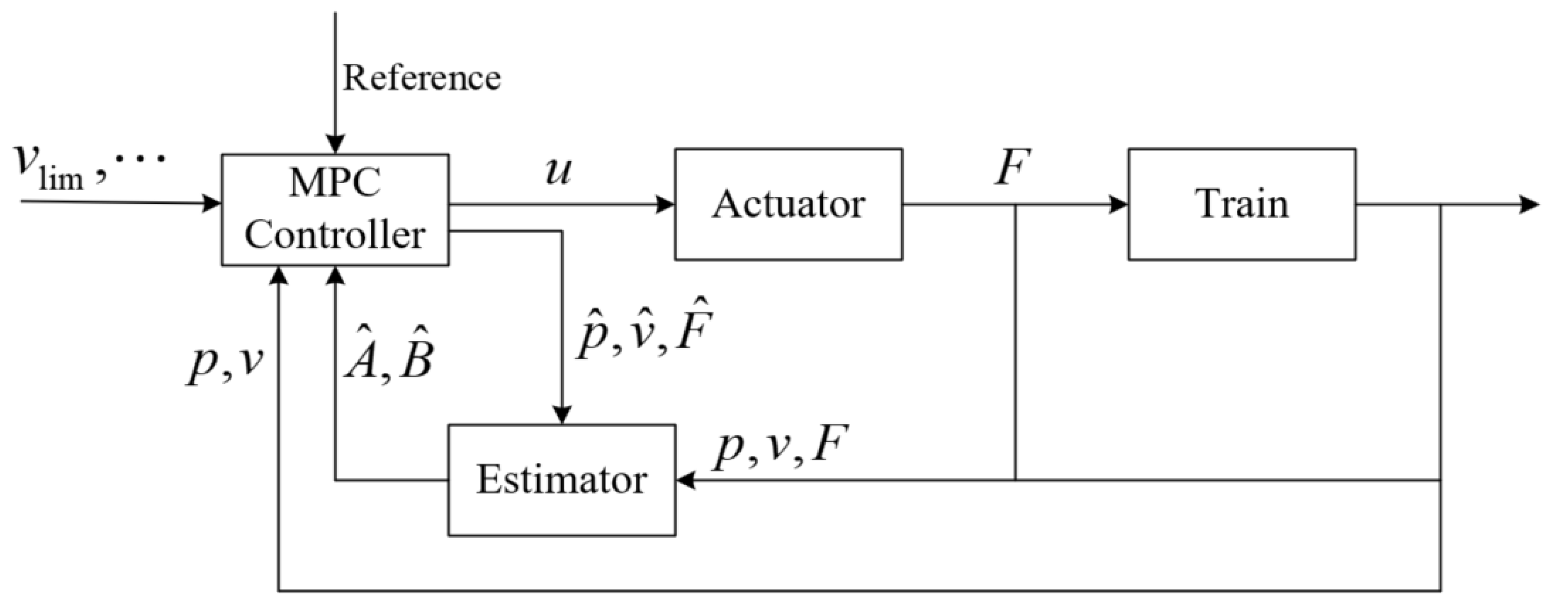
To increase the accuracy of plant model in MPC, an estimator is added into the control structure, shown in Figure 4. The predicted optimal future state and real state are transmitted to the estimated system. The function of estimator outputs an new estimated model used in the MPC controller through an adaptive updating algorithm.

The goal of the estimator of train i is to minimize the error between the predicted state and real state at time $k+1$ which can be written as a minimization problem in (32)

$${\Gamma }_i=\underset{{\widehat{\Theta }}_{i,k}}{min}{\tilde{x}}_{i,k+1}^T{\tilde{x}}_{i,k+1}$$

(32)

where ${\widehat{\Theta }}_{i,k}=\left[{\widehat{A}}_{i,k},{\widehat{B}}_{i,k},{\widehat{C}}_{i,k}\right]$, ${\tilde{x}}_{i,k+1}=x_{i,k+1|k}^{\star }-x_{i,k+1}$ and $x_{i,k+1|k}^{\star }$ is calculated by

$$x_{i,k+1|k}^{\star }={\widehat{\Theta }}_{i,k}{\chi }_{i,k}$$

(33)

where ${\chi }_{i,k}={\left[x_{i,k}^T,{u_{i,k|k}^{\star }}^T,D_{i,k}^T\right]}^T$ and

$$D_{i,k}^T=\left\{\begin{array}{c}\begin{array}{cc}I,\hfill & i=1\end{array}\hfill \\ \begin{array}{cc}{F}_{i-1,k},\hfill & t=2,3,\cdots ,N\end{array}\hfill \end{array}\right..$$

(34)

Then, (32) can be rewritten into the form related to ${\Theta }_{i,k}$ explicitly:

$${\Gamma }_i=\underset{{\widehat{\Theta }}_{i,k}}{min}{\left({\widehat{\Theta }}_{i,k}{\chi }_{i,k}-x_{i,k+1}\right)}^T\left({\widehat{\Theta }}_{i,k}{\chi }_{i,k}-x_{i,k+1}\right)$$

(35)

whose gradient with respect to ${\Theta }_{i,k}$ is

$${\nabla }_{i,k}=2\left({\widehat{\Theta }}_{i,k}{\chi }_{i,k}-x_{i,k+1}\right){\chi }_{i,k}^T.$$

(36)

The negative gradient direction is used as the updating direction for ${\widehat{\Theta }}_{i,k}$ at time k. Then, the updating law for ${\widehat{\Theta }}_i$ is presented as

$$\begin{array}{cc}\hfill {\widehat{\Theta }}_{i,k+1}& ={\widehat{\Theta }}_{i,k}-\frac{{\lambda }_{i,k}}{2}{\nabla }_{i,k}\hfill \\ \hfill & ={\widehat{\Theta }}_{i,k}-{\lambda }_{i,k}{\tilde{x}}_{i,k+1}{\chi }_{i,k}^T\hfill \end{array}$$

(37)

where $\lambda$ denotes the step of descent.

Theorem 1.

For the MPC system with an estimated model $\widehat{\Theta }$, there exits a step at each time k

$$\begin{array}{cc}{\lambda }_k=\alpha \frac{2}{{\chi }_k^T{\chi }_k},& 0<\alpha <1\end{array},$$

(38)

then, the estimated model is ultimately bounded.

Proof 

(Proof). The Lyapunov function is built as

$$V_{\widehat{\Theta }}\left(k\right)=\mathrm{tr}\left({\left({\widehat{\Theta }}_k-\Theta \right)}^T\left({\widehat{\Theta }}_k-\Theta \right)\right)$$

(39)

where $\mathrm{tr}(·)$ denotes the trace of matrix and $\Theta$ denotes the real model of plant. Based on the updating algorithm (37), the Lyapunov function follows

$$\begin{array}{cc}\hfill V_{\widehat{\Theta }}(k+1)& =\mathrm{tr}\left({\left({\widehat{\Theta }}_{k+1}-\Theta \right)}^T\left({\widehat{\Theta }}_{k+1}-\Theta \right)\right)\hfill \\ \hfill & =V_{\widehat{\Theta }}\left(k\right)+{\lambda }_k\left({\lambda }_k{\chi }_k^T{\chi }_k-2\right){\tilde{x}}_{i,k+1}^T{\tilde{x}}_{i,k+1}\hfill \end{array}$$

(40)

which is derived in [26]. Applying (38) and the Lyapunov function can be further described as

$$\begin{array}{cc}\hfill V_{\widehat{\Theta }}(k+1)-V_{\widehat{\Theta }}\left(k\right)& =2{\lambda }_k\left(\alpha -1\right){\tilde{x}}_{i,k+1}^T{\tilde{x}}_{i,k+1}\hfill \\ \hfill & \le -2{\lambda }_k\epsilon {\tilde{x}}_{i,k+1}^T{\tilde{x}}_{i,k+1}\hfill \end{array}$$

(41)

where $\epsilon$ is a constant which satisfies $\epsilon >0$. Because of ${\lambda }_k$ is a scalar which is no less than 0, it can be found that $V_{\widehat{\Theta }}(k+1)-V_{\widehat{\Theta }}\left(k\right)\le 0$. Then, with a origin $V_{\widehat{\Theta }}\left(0\right)$, the ${lim}_{k\to \infty }{V}_{\widehat{\Theta }}\left(k\right)$ exists so that the estimated model $\widehat{\Theta }$ is ultimately bounded. □

Lemma 1.

The system error $\tilde{x}$ converges to zero when $k\to \infty$, by the updating law (37).

Proof. 

We have

$$V_{\tilde{\Theta }}\left(1\right)-V_{\tilde{\Theta }}\left(0\right)=2{\lambda }_0(\alpha -1){\tilde{x}}_{i,1}^T{\tilde{x}}_{i,1},$$

(42)

$$V_{\tilde{\Theta }}\left(2\right)-V_{\tilde{\Theta }}\left(1\right)=2{\lambda }_1(\alpha -1){\tilde{x}}_{i,2}^T{\tilde{x}}_{i,2},$$

(43)

                                                            ⋮

$$V_{\tilde{\Theta }}(k+1)-V_{\tilde{\Theta }}\left(k\right)=2{\lambda }_k(\alpha -1){\tilde{x}}_{i,k+1}^T{\tilde{x}}_{i,k+1}.$$

(44)

Then we have

$$\sum _{j=0}^{k}2{\lambda }_j(\alpha -1){\tilde{x}}_{i,j+1}^T{\tilde{x}}_{i,j+1}=V_{\tilde{\Theta }}(k+1)-V_{\tilde{\Theta }}\left(0\right)$$

(45)

Because ${\lambda }_k=\alpha \frac{2}{{\chi }_k^T{\chi }_k}\ge \alpha \frac{2\alpha }{{\overline{\chi }}^2}=\overline{\lambda }$ where ${\overline{\chi }}^2\ge {\chi }^T\chi$, $\forall \chi$ which are constrained by (3)–(5). Then it follows

$$\sum _{j=0}^{k}2\overline{\lambda }(\alpha -1){\tilde{x}}_{i,j+1}^T{\tilde{x}}_{i,j+1}\le V_{\tilde{\Theta }}(k+1)-V_{\tilde{\Theta }}\left(0\right)$$

(46)

Because the ${lim}_{k\to \infty }{V}_{\tilde{\Theta }}(k+1)$ exists, so we have ${lim}_{k\to \infty }{\tilde{x}}_{i,k}\to 0$. □

Therefore, applying step (38) to the updating law (37), the model $\widehat{\Theta }$ of the plant in each local MPC controller will be ultimately bounded in a range obtained from the accurate model $\Theta$. It is more accurate than the estimated model ${\widehat{\Theta }}_0$ at origin time. Furthermore, this adaptive updating algorithm also steers the system error $\tilde{x}$ to zero.

3.4. Closing-Loop System

The proposed AMPC system with the estimator works as Algorithm 1.

Algorithm 1 Algorithm for the control system.

Input: train information $x_k$, estimated model ${\widehat{\Theta }}_k$, other essential information for MPC controller Output: train information $x_{k+1}$, estimated model ${\widehat{\Theta }}_{k+1}$ Algorithm Procedures: 1: MPC controller utilizes ${\widehat{\Theta }}_k$ to calculate a control input $u_{k|k}^{\star }$ for actuator and predict an predicted state $x_{k+1|k}^{\star }$ which is transmitted to the estimator; 2: The actuator receives $u_{k|k}^{\star }$ and acts correspondingly to generate force $F_k$, and then applies $F_k$ to the train; 3: The train outputs the system state $x_{k+1}$ at time $k+1$, which is also transmitted to the estimator; 4: The estimator receives $x_{k+1}$ and $x_{k+1|k}^{\star }$ and works with updating law (37). Then, outputs a new model ${\widehat{\Theta }}_{k+1}$ to the controller as a new model.

The AMPC system is initialized with $x_0$ and ${\Theta }_0$. Then, the closing-loop system works as Figure 5.

4. Experimental Results

The numerical experiments are consisted of two parts. One is for analysis of the performance, e.g., error value and convergent speed, of the proposed AMPCVS system in this paper. The other is an application to trains convoy, which drives in the realistic inter-station of metro.

The estimated values of uncertain parameters in the plant (11) are set as ${\widehat{c}}_0=$ $0.01$ m/s², ${\widehat{c}}_1=$ $0.005$ s⁻¹, ${\widehat{c}}_2=$ $0.0002$ m⁻¹ and $\widehat{T}=0.75$. The real values of train 1 are $c_0=$ $0.012$ m/s², $c_1=$ $0.006$ s⁻¹, $c_2=$ $0.00024$ m⁻¹, and $T=0.8$. For train 2, $c_0=$ $0.013$ m/s², $c_1=$ $0.0065$ s⁻¹, $c_2=$ $0.00026$ m⁻¹, and $T=0.8$. For train 3, $c_0=$ $0.014$ m/s², $c_1=$ $0.007$ s⁻¹, $c_2=$ $0.00028$ m⁻¹, and $T=0.8$. They are only for examples which may be not as same as some real conditions. Based on these settings, it is obvious that the real aerodynamic resistance is greater than the estimated one. Additionally, the reference speed $v_r$ in (10) can be amended by the estimator here. The weight matrices $Q_1$, $Q_i$, $P_1$, $P_i$ in optimal problem (19), (28) are set as $Q_{(·)}=I$ and $P_{(·)}=0.1I$ where I represents the unit matrix.

Remark 1.

When metro trains are under bad conditions, the air resistance becomes lager than before which implies $c_0$, $c_1$ and $c_2$ become larger. Therefore, to handle these bad conditions, the pre-set bound is supposed to be a little larger.

The rest parameters in this paper are shown in

Table 1. Parameters using in the simulation.

Parameter	Value	Unit	Parameter	Value	Unit
m	45	t	N	3	-
$u_{min}$	−54,000	N	$u_{max}$	54,000	N
$d_e$	3	m	$d_r$	5	m
L	20	m	$v_{lim}$	25	m/s

.

4.1. Adaptive Model Predictive Control Algorithm Performance

The performance of the proposed AMPC algorithm is illustrated about several aspects, including system errors and convergent speed.

Firstly, an experiment is designed here which aims at illustrating whether the proposed AMPC system is able to adjust the estimated model $\widehat{\Theta }$ to approach the real value $\Theta$. It is hard to observe the value of all the elements in the matrices of model. Then, the system error is observed here to show the performance of AMPC system. If the model in AMPC controller is close enough to the real model, the system state will converges to the objective. Additionally, the system error is in a direct proportion to the model error in AMPC controller. So, that is why we choose the system error instead of the error between the estimated model and real one.

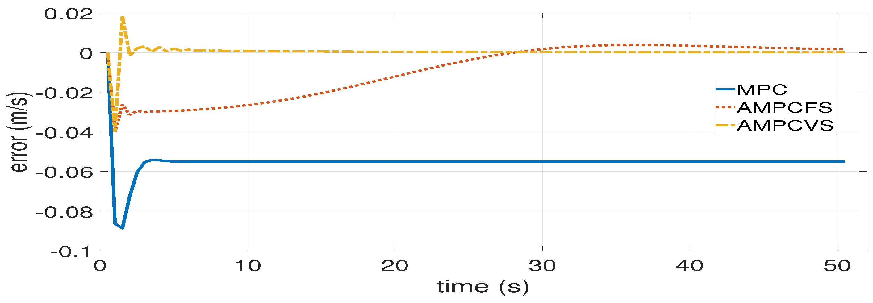
The system model in (11) is selected as an example. The objective speed for the leader is set as 20 m/s. The results of numerical experiment are shown in Figure 6. The proposed AMPC system with the variable step in this paper is abbreviated as AMPCVS. The AMPC with a fixed step proposed in [26] is abbreviated as AMPCFS.

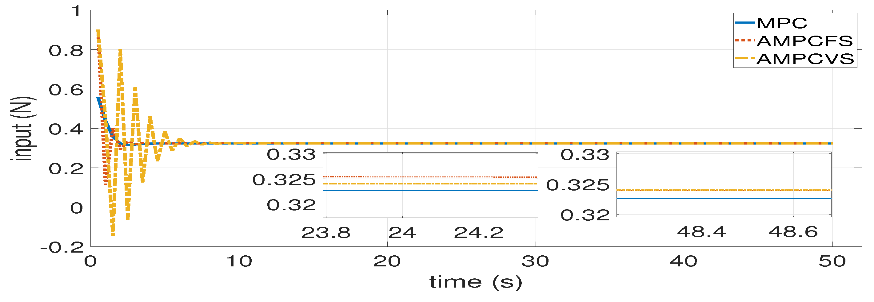
Figure 6 illustrates that all three kinds of systems make the speed converge to a value in a short time. From the figure, the speed of train with MPC system has a greater deviation from the objective than other systems. That is because the error between estimated and real values of parameters in model is not reduced, without the estimator. It can be seen from Figure 7 that the input tends to be stable because the objective function with estimated model is minimized. However, actually, the control input cannot fully compensate the resistance.

The AMPCFS system is able to converge to the objective. Because the fixed step is constrained by the system error, the fixed step has to be set as a minimum value which is related to the superior of error. Compared with the AMPCFS, the AMPCVS system converges to the objective more quickly. That is because the step is variable so that it can become greater as long as constraint allows. It is illustrated in Figure 6 that the system error of AMPCVS converges to a neighborhood rounding zero in around 3 seconds (s) but AMPCFS spends around 50 s. This result can also be found from Figure 7. The control input of AMPCVS system tends to be stable. Then, the control input of AMPCFS tends to be as same as AMPCVS.

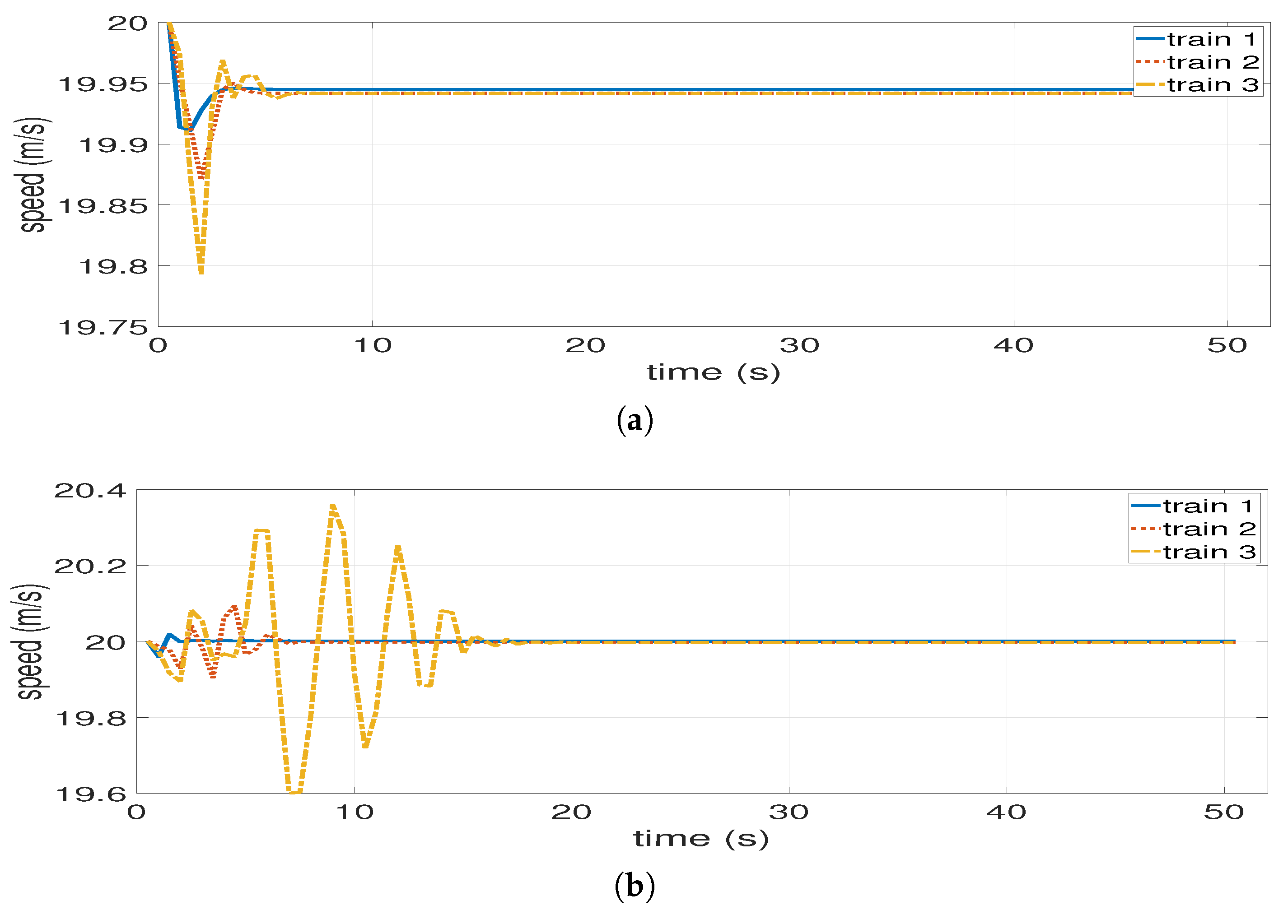
Secondly, the AMPCVS system is applied in the situation that three trains drive in VC, shown in Figure 8b. Three trains, with same property as the situation above, equipped with an MPC system are simulated as a comparison in Figure 8a. From Figure 8a, each train with an MPC system will keep a fixed speed. However, resulting from the model error, the relative speed of trains are greater than AMPCVS. The relative speed of adjacent trains causes the displacement. From Figure 9a, the distance between trains keeps increasing. It is worthwhile to notice that the objective for follower trains is keeping a constant distance from its predecessor. Thus, it is unacceptable to allow the distance to become greater (beyond communication range) or smaller (irrevocable emergent braking). The AMPCVS well regulates the distance between trains in an acceptable range, shown in Figure 9b. Although the speed of follower trains with AMPCVS varies a little more drastically than MPC, the distance keeps as desired eventually.

4.2. Inter-Station Driving of Trains in VC

Typically, trains in VC are supposed to keep a constant distance from its predecessor during the inter-station driving. Here we consider that the trains are already coupled before they depart from the station, which means the origin distance between trains equals to the desired value. Figure 10 shows the speed profile of three trains in VC driving in the inter-station with AMPCVS system.

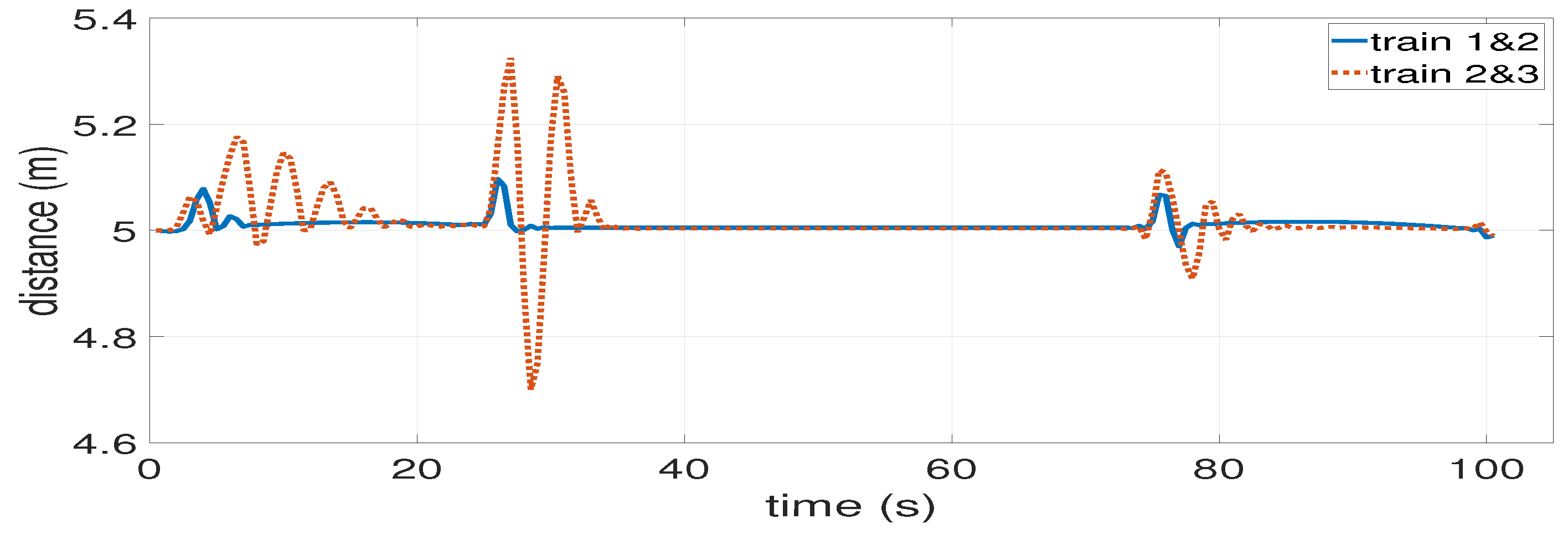
A general perception of Figure 10 is that all three trains track the reference accurately except the period that the trains are transferring from the acceleration phase to cruise. From the Figure 8b, it is easy to figure out that the system oscillates around the equilibrium point in the initial phase. The oscillation in Figure 10 is same as the characteristic shown in Figure 8b. That is because the estimator needs a certain amount of time to approach the real model of plant. After some time, the estimated model is close to the real model so that the trains track the objective well. The distance converges to the desire value shown in Figure 11. It is obviously illustrated that the distance between trains comes to the desired value in the cruise phase, i.e., from around 40 s to around 70 s.

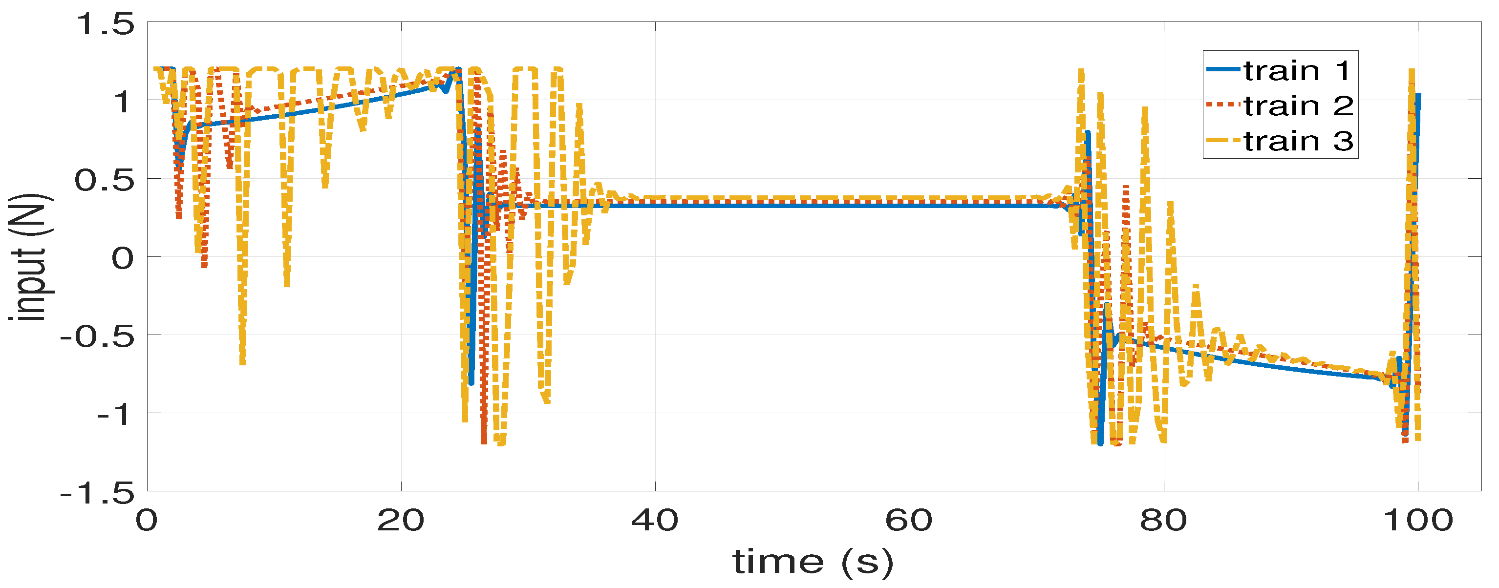
It can be seen from Figure 12 that the control input is becoming greater. It results from the increasing aerodynamic resistance, which is in a direct proportion to speed. The control input needs to be increased correspondingly in order to counteract the increasing resistance.

The control input is adjusted with respect to the distance between trains. The oscillation of distance makes the control input vary drastically. Once the distance become smaller than the desired value, the control input decreases to make the train slower than its predecessor and vice versa. It is greater than zero, except the braking phase, which counteracts the resistance with respect to the different condition and steer train to the desired state. The distance error oscillates in the traction phase, however, the peak values of distance error become smaller in order. This characteristic is also reflected in control input. The peak values of control input, in one operation phase, also become smaller in order. That is because the estimated model approaches the real value step by step over time. So that, if the model is accurate enough, it will hardly change anymore. Then, once the distance becomes the desire, the control input maintains a fixed value. Regarding the different parameters of three trains, the input force to maintain a desired speed is different in the cruise phase. The required control input for train 3 to maintain desired speed should be greatest, corresponding to the simulation setting. It is exactly observed in Figure 12.

Another phenomenon is that the peak distance error of train 2 and 3 is greater than train 1 and 2, shown in Figure 11. That is because the error of predecessor is accumulated to the follower so that the performance of estimator in follower is degraded. The follower need spend more time than its predecessor to reach the equilibrium point.

Remark 2.

The parameters $c_0$, $c_1$, and $c_2$ are set as unknown but fixed values in the numerical experiment here. However, $v_r$ is a variable with respect to the current speed of train which is a time-varying parameter for AMPCVS system. This condition happens when the speed of train is changing (accelerating and decelerating). From the illustration above, we can figure out that the AMPCVS system deals with this kind of time-varying parameters well, i.e., steering the system to desired states. Thus, the AMPCVS system may also deal with other slow time-varying parameters like time varying $c_0$, $c_1$, and $c_2$.

5. Conclusions

We propose a distributed AMPC system for trains in VC in this paper. An estimator is designed for each local controller, which makes the estimated model adaptive and accurate. A gradient descent method with a variable descent step steers the estimated values of parameters to real ones. Simulations are conducted and the results of our proposed AMPCVS are compared with both nominal MPC and AMPCFS. The error between actual distance and desired ones in our algorithm is much smaller than the nominal MPC, and the error converges to zero most quickly among three. These indicate an improvement of AMPCVS algorithm when compared with other two systems. An entire running process in an inter-station with our proposed AMPCVS is also simulated. Experimental results show that the trains track the desired objective well.

In the future work, we will try to alleviate the oscillations during a control process. Another direction is to design an adaptive MPC system considering system disturbances, where the theory of positively invariant set [30] and robust MPC [31] may be combined with the adaptive scheme. Considering the huge energy cost of a metro system [32], an integrated dispatching and control system which makes full use of VC to increase the track capacity while saving energy is also to be designed in the future.

References

1. Quaglietta, E.; Wang, M.; Goverde, R.M.P. A multi-state train-following model for the analysis of virtual coupling railway operations. J. Rail Transp. Plan. Manag. 2020, 15, 1–14. [Google Scholar]
2. Bock, U.; Varchmin, J. Enhancement of the occupancy of railroads using ‘virtually coupled train formations’. In Proceedings of the World Congress Railway Research, Tokyo, Japan, 19–23 October 1999; pp. 1–7. [Google Scholar]
3. Bock, U.; Bikker, G. Design and development of a future freight train concept—“virtually coupled train formations”. In Proceedings of the IFAC Control in Transportation Systems, Braunschweig, Germany, 13–15 June 2000; pp. 1–6. [Google Scholar]
4. Konig, S.; Schnieder, E. Modeling and simulation of an operation concept for future rail traffic. In Proceedings of the IEEE Intelligent Transportation Systems Conference, Oakland, CA, USA, 25–29 August 2001; pp. 808–812. [Google Scholar]
5. Haltuf, M. Shift2Rail JU from member state’s point of view. Transp. Res. Procedia 2016, 14, 1819–1828. [Google Scholar] [CrossRef]
6. Flammini, F.; Marrone, S.; Nardone, R.; Petrillo, A.; Santini, S.; Vittorini, V. Towards railway Virtual Coupling. In Proceedings of the IEEE International Conference on Electrical Systems for Aircraft, Railway, Ship Propulsion and Road Vehicles & International Transportation Electrification Conference, Nottingham, UK, 7–9 November 2018; pp. 1–6. [Google Scholar]
7. Henke, C.; Tichy, M.; Schneider, T.; Böcker, J.; Schäfer, W. Organization and control of autonomous railway convoys. In Proceedings of the 9th International Symposium on Advance Vehicle Control, Kobe, Japan, 6–9 October 2008; pp. 1–6. [Google Scholar]
8. Goikoetxea, J. Roadmap towards the wireless Virtual Coupling of trains. In Proceedings of the International Workshop on Communication Technologies for Vehicles, San Sebastian, Spain, 6–7 June 2016; pp. 3–9. [Google Scholar]
9. Xu, X.; Song, Z. Study on Train Control Technology in Virtual Coupling Concept. In Proceedings of the World Congress Railway Research, Tokyo, Japan, 28 October–1 November 2019; pp. 1–7. [Google Scholar]
10. Felez, J.; Kim, Y.; Borrelli, F. A model predictive control approach for Virtual Coupling in railways. IEEE Trans. Intell. Transp. Syst. 2019, 20, 2728–2739. [Google Scholar] [CrossRef]
11. Gao, S.G.; Dong, H.R.; Ning, B.; Clive, R.; Chen, L.; Sun, X.B. Cooperative adaptive bidirectional control of a train platoon for efficient utility and string stability. Chin. Phys. B 2015, 24, 1–10. [Google Scholar] [CrossRef]
12. Bai, W.; Lin, Z.; Dong, H.R.; Ning, B. Distributed cooperative cruise control of multiple high-speed trains under a state-dependent information transmission topology. IEEE Trans. Intell. Transp. Syst. 2019, 20, 2750–2763. [Google Scholar] [CrossRef]
13. Saxena, A.; Li, H.; Goswami, D.; Math, C.B. Design and analysis of control strategies for vehicle platooning. In Proceedings of the 19th IEEE Intelligent Transportation Systems, Rio de Janeiro, Brazil, 1–4 November 2016; pp. 1805–1812. [Google Scholar]
14. Marais, J.; Beugin, J.; Berbineau, M. A survey of GNSS-based research and developments for the European railway signaling. IEEE Trans. Intell. Transp. Syst. 2018, 10, 2602–2618. [Google Scholar] [CrossRef] [Green Version]
15. Cai, B.; Wu, B.; Lu, D. Survey of performance evaluation standardization and research methods on GNSS-based localization for railways. Chin. J. Electron. 2020, 29, 22–33. [Google Scholar] [CrossRef]
16. Gómez, A.; Mozoet, E.; Bernadó, L.; Zelenbaba, S.; Thomas Zemen, T.; Parrilla, F.; Alberdi, A. Performance Analysis of ITS-G5 for Smart Train Composition Coupling. In Proceedings of the 16th International Conference on Intelligent Transportation Systems Telecommunications, Lisboa, Portugal, 15–17 October 2018; pp. 1–7. [Google Scholar]
17. Zhao, J.; Liu, J.; Yang, L.; Ai, B.; Ni, S. Future 5G-oriented system for urban rail transit: Opportunities and challenges. Chin. Comm. 2021, 18, 1–12. [Google Scholar] [CrossRef]
18. Di Meo, C.; Di Vaio, C.; Flammini, F.; Nardone, R.; Santini, S.; Vittorini, V. ERTMS/ETCS Virtual Coupling: Proof of concept and numerical analysis. IEEE Trans. Intell. Transp. Syst. 2020, 21, 2545–2556. [Google Scholar] [CrossRef]
19. Park, J.; Lee, B.H.; Eun, Y. Virtual Coupling of railway vehicles: Gap reference for merge and separation, robust control, and position measurement. IEEE Trans. Intell. Transp. Syst. 2020. [Google Scholar] [CrossRef]
20. Mayne, D.Q. Constrained model predictive control: Stability and optimality. Automatica 2000, 36, 789–814. [Google Scholar] [CrossRef]
21. Mayne, D.Q. Model predictive control: Recent developments and future promise. Automatica 2014, 50, 2967–2986. [Google Scholar] [CrossRef]
22. Lu, Y.; Arkun, Y. Quasi-Min-Max MPC algorithms for LPV systems. Automatica 2000, 36, 527–540. [Google Scholar] [CrossRef]
23. Mayne, D.; Raković, S.V.; Findeisen, R.; Allgöwer, F. Robust output feedback model predictive control of constrained linear systems. Automatica 2006, 42, 1217–1222. [Google Scholar] [CrossRef]
24. Mayne, D.; Raković, V.S.; Findeisen, R.; Allgöwer, F. Robust output feedback model predictive control of constrained linear systems: Time varying case. Automatica 2006, 45, 2082–2087. [Google Scholar] [CrossRef]
25. Xie, L.; Xie, L.; Su, H. A comparative study on algorithms of robust and stochastic MPC for uncertain systems. ACTA Autom. Sin. 2017, 43, 969–992. [Google Scholar]
26. Zhu, B.; Xia, X.H. Adaptive model predictive control for unconstrained discrete-time linear systems with parametric uncertainties. IEEE Trans. Autom. Control 2016, 61, 3171–3176. [Google Scholar] [CrossRef]
27. Chai, R.; Savvaris, A.; Tsourdos, A.; Chai, S.; Xia, Y. Optimal tracking guidance for aeroassisted spacecraft reconnaissance mission based on receding horizon control. IEEE Trans. Aerosp. Electr. Syst. 2018, 54, 1575–1588. [Google Scholar] [CrossRef] [Green Version]
28. Xu, X.; Peng, J.; Zhang, R.; Chen, B.; Zhou, F.; Yang, Y.Z.; Gao, K.; Huang, Z.W. Adaptive model predictive control for cruise control of high-speed trains with time-varying parameters. J. Adv. Transp. 2019, 2019, 7261726. [Google Scholar] [CrossRef]
29. Negenborn, R.R.; Schutter, B.; Hellendoorn, J. Efficient implementation of serial multi-agent model predictive control by parallelization. In Proceedings of the IEEE International Conference on Networking, Sensing and Control, London, UK, 15–17 April 2007; pp. 175–180. [Google Scholar]
30. Raković, S.; Kerrigan, E.; Kouramas, L.; Mayne, D. Invariant approximations of the minimal robust positively invariant set. IEEE Trans. Autom. Control 2005, 50, 406–410. [Google Scholar] [CrossRef] [Green Version]
31. Mayne, D.Q.; Seron, M.M.; Raković, S.V. Robust model predictive control of constrained linear systems with bounded disturbances. Automatica 2005, 41, 219–224. [Google Scholar] [CrossRef]
32. Su, S.; Wang, X.; Cao, Y.; Yin, J. An energy-efficient train operation approach by integrating the metro timetabling and eco-driving. IEEE Trans. Intell. Transp. Syst. 2020, 21, 4252–4268. [Google Scholar] [CrossRef]
Figure 1. Communication structure between trains in VC.
Actuators 10 00178 g001
Figure 2. Distributed control structure for N trains in VC.
Actuators 10 00178 g002
Figure 3. Serial distributed MPC control structure for two trains.
Actuators 10 00178 g003
Figure 4. Adaptive MPC control system.
Actuators 10 00178 g004
Figure 5. Closing-loop system flows.
Actuators 10 00178 g005
Figure 6. The speed profile of train with different MPC systems.
Actuators 10 00178 g006
Figure 7. The control input of train with different MPC systems.
Actuators 10 00178 g007
Figure 8. Comparison of speed profile. (a): The speed profile of trains with MPC system. (b): The speed profile of trains with AMPCVS system.
Actuators 10 00178 g008
Figure 9. Comparison of distance between trains. (a): The distance between trains with MPC system. (b): The distance between trains with AMPCVS system.
Actuators 10 00178 g009
Figure 10. The speed profile of trains in VC driving on inter-station with AMPCVS system.
Actuators 10 00178 g010
Figure 11. The distance of trains in VC driving on inter-station with AMPCVS system.
Actuators 10 00178 g011
Figure 12. The control input of trains in VC driving on inter-station with AMPCVS system.
Actuators 10 00178 g012