Abstract
Heavy-haul trains have the characteristics of large volume, long formation, and complex line conditions, which increase the driving difficulty of drivers and can easily cause safety problems. In order to improve the safety and efficiency of heavy-haul railways, the train control mode urgently needs to be developed towards the direction of automatic driving. In this paper, we take the Shuohuang Railway as the research background and analyze the train operation data of SS4G locomotives. We find that the proportion of operation data under different working conditions is seriously out of balance. Aiming at this unbalanced characteristic, we introduce the classification method in the field of machine learning and design an intelligent driving algorithm for heavy-haul trains. Specifically, we extract the data by random forest algorithm and compare the classification performance of C4.5 and CART algorithms. We then select the CART algorithm as the base classifier of the AdaBoost algorithm to build the model of the automatic air brake. For the purpose of heightening the precision of the model, we optimize the AdaBoost algorithm by improving the generation of training subsets and the weight of voting. The numerical results certify the effectiveness of our proposed approach.
1. Introduction
Heavy-haul railways have the characteristics of large capacity, high efficiency, low energy consumption, and low transportation costs and are widely valued by countries all over the world. They have been recognized internationally as the main direction of the development of railway bulk cargo transportation. For China, the United States, Canada, and other continental countries with vast territory, rich products, and uneven distribution of resources, the development of heavy-haul railways will help to rapidly increase transportation capacity, alleviate transportation bottlenecks, and improve transportation economic benefits.
Shuohuang Railway Line is a typical heavy-haul railway line, which is an important coal transportation line in the Chinese West Coal East Transport Project. Like other heavy-haul railway lines, although its driving plan is fixed, the line conditions are very complex, e.g., there are many long and steep downhills along the railway line. A driver of a heavy-haul train usually has to follow a predefined driving curve, which leads to great pressure on the drivers [1,2,3].
Automatic train operation (ATO) has been widely used in urban rail transit systems, which realizes the complete automation of the work performed by train drivers and the highly centralized control of trains. Research shows that if the ATO system were to be applied to heavy-haul trains, the workload of the drivers would be greatly reduced, and the safety and operation efficiency would be greatly increased [4].
At present, the research on the automatic driving of urban rail transit trains is very mature, and the relevant algorithms of train automatic control include PID classic control theory, genetic algorithm, fuzzy control theory, machine learning, and so on. Gruber and Bayoumi [5] achieve curve tracking with the goal of minimizing the coupling force caused by disturbances such as slope. Hou [6] introduced the TILC method to the automatic stopping of the train when entering the station and used the error of the terminal stop position during the previous braking process to update the current control curve. The authors of [7] introduce GA to generate optimal idle control based on punctuality, comfort, and energy consumption.
Furthermore, many studies have introduced fuzzy control into the control of freight trains. Bonissone et al. synthesized a fuzzy controller to track the speed curve while driving smoothly within the speed limit and used genetic algorithms to adjust the parameters of the fuzzy controller (scaling factor and membership function) to optimize the performance of the fuzzy controller [8]. Sekine [9] uses a fuzzy controller to control the speed of coal trains during unloading operations to keep it constant. The literature shows that fuzzy controllers can be successfully applied to specific control tasks.
Based on the historical data of train stops, Bai [10] modeled the latest status of train braking equipment and introduced fuzzy neural networks to realize intelligent control of freight train stops. Reinforced learning, as a variant of the Markov decision process [11], also shows good characteristics in train control. Based on the channel characteristics of the CBTC communication system and real-time train position information, Zhu Li uses deep reinforcement learning to achieve joint optimization of communication performance and a train control strategy [12]; based on transponder positioning information, Chen Dewang et al. modeled train control into multiple models. In the stage of the decision-making process, the reciprocal of the parking error is set as the return value, and reinforcement learning is introduced to solve the maximum return function [13].
Yet, the research on autonomous driving of heavy-haul trains is relatively rare. Because heavy-haul trains do not have linear time-varying braking and traction systems, they cannot be described by PID control systems. At the same time, due to the flexible formation of heavy-haul trains, it is not possible to generalize the application of fuzzy control models. Machine learning has strong adaptability and a nonlinear processing ability and can learn characteristics of train operation data at different marshaling [12,14].
Thus, it becomes possible to apply machine learning in the intelligent driving of heavy-haul trains. However, there are still some problems to overcome, such as the possibility of being trapped in a local optimal solution, slow convergence speed, and ease of overfit. Therefore, this paper uses classification algorithms in data mining and machine learning to build a model of an intelligent heavy-haul train air braking system and to predict different driving strategies.
The main contributions of this paper are as follows:
- A random forest algorithm is introduced to reduce the dimensionality of the characteristics of the heavy-haul train operation data.
- An AdaBoost-based algorithm is designed to realize the intelligent control of the air brake of the heavy-haul trains.
- We optimize the AdaBoost algorithm from two aspects: the extraction method of the training sample subset and the voting weight. Finally, the highly precise control of the air brake and the intelligent driving of heavy-haul trains are realized.
The rest of the paper is organized as follows. Section 2 introduces the main procedures of the machine-learning-based heavy-haul train intelligent driving method. In Section 3, we introduce the work of data pre-processing. Then, we use the random forest algorithm to extract features in Section 4. In Section 5, we propose the AdaBoost algorithm to build the heavy-haul train air braking model. Then, we present the numerical results in Section 6 and finally make a conclusion in Section 7.
2. Main Procedures of the Machine-Learning-Based Heavy-Haul Trains Intelligent Driving Method
Research shows that air braking mainly refers to several different amounts of decompression to control trains [15]; this paper combines machine learning with classification algorithms in the heavy-haul train air braking intelligent control system. Machine learning processes generally include the following steps.
2.1. Modeling
First, the problems studied in this paper are turned into the mathematical model of machine learning. The intelligent control of heavy-haul trains can be divided into two parts: intelligent control of air braking and intelligent control of electric braking. The pressure values applied to the air brake are discrete; thus, this control process could be defined as a classification problem in machine learning.
2.2. Data Collection
In this paper, the relevant data on the route are collected from Shenchi South Station to Suning North Station of the Shuohuang Railway, including information on the train operation characteristics and line features.
2.3. Data Pre-Processing
In this step, we delete incorrect data from the collected data to make it easy to be calculated. In addition, in order to better supervise learning, the feature labels not collected need to be supplemented.
2.4. Feature Extraction
In order to improve the algorithmic performance, it needs to select the correct features for training and learning, and this paper completes feature extraction engineering by building, extracting, and selecting features in the original data set, which is a basic step of mining data in the field of machine learning. A total of 17 important features are selected in this paper.
2.5. Model Training and Optimization
This paper uses the classification learning algorithm to train the intelligent control model of heavy-haul trains. Firstly, we use the AdaBoost algorithm to learn the characteristic space of the train operating data, and then we adjust the data quantity and the parameters used in the algorithm, so as to optimize the model, and finally encapsulate the model. The processes are shown in Figure 1.
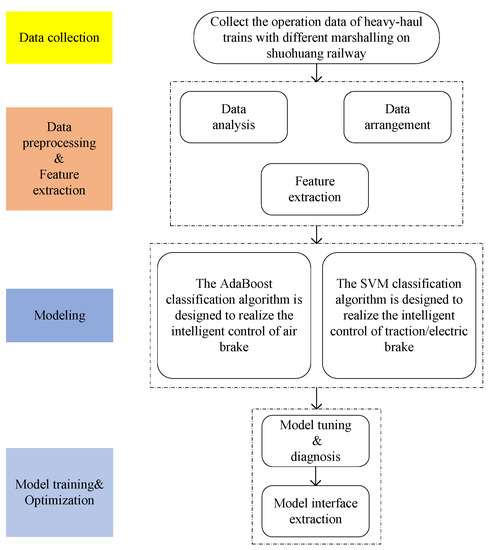
Figure 1.
A flowchart for intelligent driving of heavy-haul trains based on machine learning.
3. Data Pre-Processing
The data collected from the heavy-haul trains contain errors and anomaly points, as well as random noise during acquisition, which can adversely affect the results. The static and dynamic data collected are not perfect enough, and the missing data must be supplemented. Therefore, the initial collected data need to be pre-processed, including data standardization and data complementation.
3.1. Data Analysis
Analysis of the initial data shows the collected information about the trains in Table 1. This paper collected a total of 35 items of static line information, such as line slope, speed limit, and other information.

Table 1.
Collected information.
3.2. Data Complement
The cycle of data collection by on-board equipment is not uniquely determined but is triggered by events such as the different operating strategies or the different operating conditions. Thus, data omissions or loss may occur during the processes of collecting data, and they can be matched by asking for the average value of the location context data [16,17]. However, in practical applications, air brake decompression, the indicator closely related to air braking, is not collected and cannot be complemented by the above method. Therefore, we design a special algorithm to supplement it.
By studying the air braking system of heavy-haul trains, it can be known that when air braking is applied, the train tube will drain air. When the air brake is released, the air will slowly enter the train’s tube. Therefore, by calculating the pressure difference between the train cylinder in full air and in applied air brake, we will obtain the air brake decompression [18]. The algorithm is shown in Algorithm 1.
| Algorithm 1 An air brake decompression calculation method |
|
3.3. Data Normalization
We collect a wide range of data, whose scales are at different levels, which will lead to disunity calculation, so the data need to be standardized at the same level. Then, the training speed and accuracy of the model will be improved.
We select the Z-score normalization algorithm, and the formula is shown in Formula (1):
where is the mean of the sample data, and is the standard deviation of the sample data.
3.4. Analysis of Unbalanced Data
Data unbalance refers to the large difference between the number of samples of one type and other types in the entire sample set. Samples can then be divided into majority and minority categories based on the sample size. Typically, when the ratio of the number of minority classes to majority classes is less than 1:2, this means that the data are unbalanced for the sample set [19].
Figure 2 shows a map of the air brake applied by an expert driver between Shenchi South Station and Suning North Station. As can be seen from the figure, air braking is not required all the time while the train is operating, and it is needed only in a few cases, because air braking is applied only when the train speed cannot reduce to the speed limit by electric braking on a long downhill slope. In all the data, the ratio of samples with air brake output to samples without air brake output is 1:6, where the ratio of samples with 80 kPa of decompression to samples without air brake output is 1:15, so the data are seriously unbalanced.
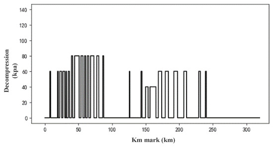
Figure 2.
The air brake output by the expert driver.
For the classification of unbalanced datasets, in order to minimize the rate of misclassifying, general classifiers tend to focus on the classification effect of majority classes, while ignoring the classification effect of minority classes [20].
In summary, although the need to apply air braking falls into a minority category, its failure can have serious safety problems, such as speeding, decoupling, and other major accidents, which will result in huge losses. Therefore, in view of the imbalance of train operation data, this paper designs a classifier that can highly and accurately identify majority and minority classes and realize the intelligent driving of heavy-haul trains.
4. Feature Extraction of Heavy-Haul Train Operation Data Based on Random Forest
The relevant data collected by the on-board devices contain several types of information; on the one hand, these multi-dimensional features improve the performance of the classifier, but on the other hand, they also increase the complexity of the algorithm, and it is possible to cross the critical point and thus deteriorate the performance of the classifier [21]. Therefore, this paper uses the random forest algorithm to extract the characteristics of the train operation data and selects the characteristics that affect the air braking of the train more substantially, so as to avoid the effect of data redundancy.
4.1. Random Forest Algorithm
The random forest algorithm generates a new set of samples by randomly taking K samples in the original sample set and then uses these new sample sets to generate K classification trees, which is used to determine the final classification decision by synthesizing the classification results of the K classification trees. This random use of features and samples allows the role of each feature to be evaluated when training each tree, resulting in better classifier performance after synthesis [22]. The processes of establishing a random forest are shown in Figure 3.
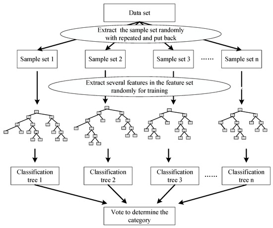
Figure 3.
The process of establishing a random forest.
4.2. Air Braking Modeling of Heavy-Haul Trains Based on Random Forests
We first set two types of labels, that is, for the need to apply air braking and for no need to apply air braking. Then, we use the collected train operation information and line information as a training feature set and use the random forest algorithm to build a better performance classifier, so as to obtain the 10th degree of ability of each indicator. The specific processes are shown as follows:
- Data pre-processing.According to the method described in Section 3, we first complement and normalize the data and then combine the train operation data with the static line information.
- Randomly extract sample sets.In this step, we randomly select 70 data sets from Shenchi South Station to Suning North Station on the Shuohuang Railway as the training sample set and randomly extract 2/3 of the data from the entire sample set each time through replacement. Finally, we extract a total of 100 new data sets as .
- Randomly extract feature sets.We use the above 100 new data sets to build 100 decision trees to form a random forest. Each decision tree contains five layers, and the random forest does not need to be pruned. Because the random extraction of sample sets and feature sets has been guaranteed randomness, the resulting random forest will not appear over-fitting. Each tree has 15 non-leaf nodes, that is, 1500 nodes need to be branched, so as to extract 1500 random feature sets as the basis for node branching.The collected data set contain 35 indicators, 1/3 of which is selected as the reference feature of each node, that is, the number of features at each node is 11. Eleven features are randomly selected from the entire feature set as a new feature set as , and 1500 sets are extracted to form the training feature set.
- Build a decision tree.In this step, we use the process described in Section 5 to construct a CART decision tree. Each decision tree uses the data sets obtained in step 2. The feature set considered at each node in the decision tree is selected in turn from step 3 to construct 100 CART decision trees.
- Build a random forest.Finally, we use the 100 decision trees constructed above to combine a random forest through voting.
When the random forest construction is completed, we will quantify the contribution value of the feature by using the Gini coefficient, and if the feature is used for the division of a node in the decision tree, we then calculate the change value of the Gini coefficient before and after the split at the node. Finally, we add the change value of the Gini coefficient of all nodes that use the feature for division as the contribution value of the feature. The expression of the Gini coefficient is shown in Formula (2).
where is the proportion of K category at node m, .
On this basis, the final contribution evaluation value can be obtained, and the processes are as follows:
- Firstly, we calculate the contribution value of feature at the node, that is, the change of Gini impurity before and after the node branch:where and denote the Gini impurity of the nodes corresponding to the left and right subtrees of node m after branching.
- Secondly, if feature is extracted during the training process of decision tree i, then we can compute the importance of in the tree:where M refers to the set of nodes where feature appears in decision tree i.
- When there are n trees in the random forest, we can calculate the contribution value of feature in the random forest:
- Finally, we normalize the obtained contribution value to obtain the final contribution evaluation value:
After obtaining the quantified value of each feature contribution and sorting from largest to smallest, we select the features with the contribution value in the top 1/3 as the feature set for the final model training, and the first 17 are selected as candidate features. When the subsequent model selects features, the feature with the smallest contribution value is sequentially deleted from the candidate feature set using the backward elimination method for training until the optimal model is obtained [23].
4.3. Analysis of the Feature Extraction Results
In this paper, the number of decision trees is 100, and the number of decision trees is constantly adjusted to make the performance of random forests better. The relationship between the number of different decision trees and random forest performance is shown in Table 2.
Table 2.
The relationship between the number of decision trees and the performance of random forests.
As can be known from Table 2, when the number of decision trees is 250, the performance requirements of feature extraction are met, so we select the top 17 features as an alternative feature set when the number of decision trees is 250. Furthermore, as can be known from Figure 4, the 17 characteristics such as slope, speed, and target distance have a great influence on whether it is necessary to output air braking. Thus, we use the extracted 17 features as a feature set and construct a random forest again. The quantified performance of the random forest is shown in Table 3.
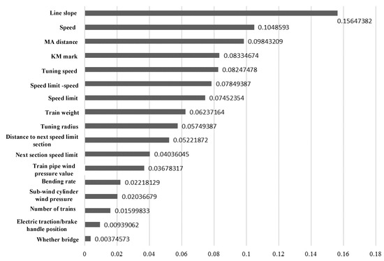
Figure 4.
Contribution value of the features.
Table 3.
The relationship between the number of decision trees and random forest performance after feature extraction.
As can be found in Table 3, the classification effect of the random forest classifier is obviously improved after feature extraction, but the prediction effect is still far from good enough, so the AdaBoost algorithm is introduced to further optimize.
5. AdaBoost-Based Intelligent Control Algorithm for Air Braking on Heavy-Haul Trains
5.1. AdaBoost Algorithm
Heavy-haul trains have strong inertia due to their large mass, so air brakes are used instead of electric brakes as the main braking force to ensure a short braking distance. Through the preliminary analysis of data, the decompression of the air brake is mainly concentrated among 40 kPa, 60 kPa, 80 kPa, 100 kPa, 120 kPa, and 140 kPa. In this paper, the intelligent control of the air brake of the heavy-haul trains is modeled as a multi-class problem. The different gears that do not need to apply the air brake and those that apply the air brake are used as class labels of the classifier, and the model outputs the operation strategies in different states through the extracted feature set to realize the intelligent control of the train air brake.
However, the trains do not need to apply air brakes most of the time during operation. When the trains are on a long downhill slope, the electric brake alone cannot control the train speed below the speed limit. At this time, the driver will consider applying the air brake. Such characteristics mean that the Shuohuang Railway operating data presents a typical imbalance with respect to the air brake output, among which the category of applying the air brake belongs to a minority category.
For such an unbalanced data set, the traditional classifier algorithm cannot achieve high-precision prediction of minority classes. Just as the random forest algorithm used in Section 4 has a poor prediction effect, the scene that needs to output the air brake is misjudged as not needing to be applied, posing a major threat to the safe operation of trains. The AdaBoost algorithm has a high degree of recognition for unbalanced data sets. This paper introduces the AdaBoost algorithm into the intelligent control of the air brake of heavy-haul trains. AdaBoost is a kind of ensemble boosting algorithm, which constructs a strong classifier through several weak classifiers. The weak classifier here means that the performance of the classifier is better than the result of random prediction, that is, the accuracy of the classifier is more than 50%. The AdaBoost algorithm allows the weak classifier to continue to expand until the error rate reaches a certain set value.
AdaBoost is an iterative algorithm that first samples the training sample set by random sampling and then obtains different subsets. Then, it uses these different subsets to train different base classifiers and finally combines the base classifiers to obtain the final strong classifier through voting.
Since the samples are typically unbalanced data sets, and traditional classifier algorithms can only implement high-precision predictions for majority classes and ignore minority classes, an AdaBoost algorithm is adopted to solve this problem effectively.
AdaBoost needs to solve the problem through continuous iteration. The first step of the algorithm is random sampling. In the second step, we train the base classifier with each subset obtained from the samples. The third step is to obtain a strong classifier based on the weight combination of these base classifiers [24]. The AdaBoost algorithm flow is shown in Figure 5. The base classifier selected in this paper is the decision tree algorithm, which is a tree structure with multiple nodes, among which each internal node represents a test on a property, each branch represents a test output, each leaf node represents a category, and the last leaf node represents the final result. The classification results are obtained by training the data in the sample space and judging their characteristics.
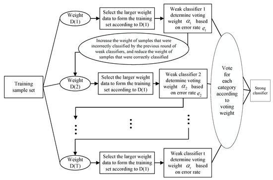
Figure 5.
A flow of the AdaBoost algorithm.
The key issue of applying the decision tree algorithm is which feature in the data set plays a decisive role in node classification, that is, the selection of features at each non-leaf node. Therefore, each feature must be evaluated. This process is called the feature selection process of the algorithm. According to the difference of feature selection, commonly used decision tree algorithms include the C4.5 algorithm and CART algorithm. This paper applies these two algorithms to the study of air brake selection strategies for heavy-haul trains and selects a more suitable algorithm through comparison. The comparison and analysis of simulation results between C4.5 and CART are introduced in Section 5.2.
5.2. Comparison and Analysis of Simulation Results between C4.5 and CART Algorithms
We use the C4.5 and CART algorithms to model the decompression amount applied to the air brake during the operation of the heavy-haul trains to realize its intelligent control. The air brake decompression volume is concentrated among 0 kPa, 40 kPa, 60 kPa, 80 kPa, 100 kPa, 120 kPa, and 140 kPa. Therefore, this article regards these seven category labels as the final air brake pressure reduction output decision Y. In addition, the 17 key features extracted in Section 4 are selected as the feature set of the model . In this way, an 18-dimensional array composed of feature sets and class labels is obtained, 2/3 of the data in the array is randomly selected as the training sample set, and the remaining data are used as the test sample set to build two decision tree models.
The number of seven categories in the data set is shown in Table 4. When randomly sampling the training sample set and the test sample set, randomly sample 2/3 of the data of each category as the training sample set to ensure the number of minority samples.
Table 4.
Number of samples for each category in the data set.
The C4.5 algorithm model and the CART algorithm model are obtained through the training of the training sample set for the two decision numbers, and the two models are used to predict the test data set. The verification results are for different air brake output prediction accuracy comparisons. As shown in Figure 6, it can be seen that the accuracy of the two algorithms has a small difference. Due to the imbalance of the data, this indicator cannot fully evaluate the accuracy of the model.
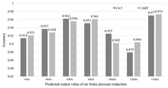
Figure 6.
Prediction precision of C4.5 and CART algorithms.
The predicted recall rates of the two algorithms for different air brake outputs are shown in Figure 7. From the figure, it can be seen that the recall rate of the CART algorithm is significantly higher than that of the C4.5 algorithm in the prediction of the need to output the air brake. That is, when air brakes need to be applied, CART’s predictive performance is better.
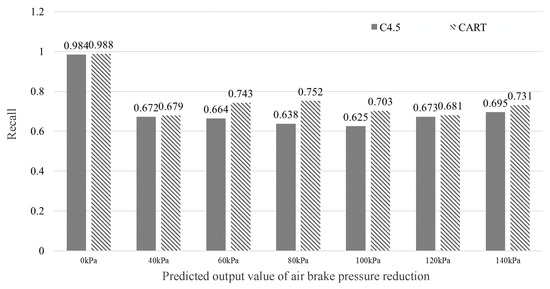
Figure 7.
Prediction recall of C4.5 and CART algorithms.
In addition to the above experimental results, in terms of execution efficiency, the C4.5 algorithm uses information gain rate selection features and makes judgments based on the entropy model of information theory. In the calculation process, a large number of logarithmic operations will be designed, and the computer consumes a lot of resources. Whether it is in the model training stage or the final use of the model to predict unknown data, there is a problem of low efficiency. The CART algorithm is more of a square operation, which is more efficient. It is possible that a single decision tree cannot reflect the difference in efficiency, but after a large number of decision trees are integrated through AdaBoost, the performance difference will be magnified, even reaching the level of tens of milliseconds. In the process of heavy-haul train operation, in order to make faster adjustments to the real-time environment and ensure the safety of train operation, the CART algorithm, as the base classifier, undoubtedly has higher execution efficiency.
In summary, the CART algorithm has obvious advantages over the C4.5 algorithm in terms of the prediction effect reflected by the experimental results and the execution efficiency of the theoretical analysis. Thus, we ultimately use the CART decision tree algorithm as the base classifier of the AdaBoost ensemble algorithm.
5.3. CART Model Building
The CART decision tree algorithm uses a binary split binary tree, which divides the data set by using a feature threshold and uses the Gini coefficient as an evaluation indicator when selecting the best split point [25]. The Gini coefficient describes the purity of the data set: the larger the Gini coefficient, the less pure the data, and the smaller the Gini coefficient, the more uniform the data set. Each iteration of the CART algorithm produces a feature that reduces the Gini coefficient after the data are divided, so that the classification effect of the dataset is gradually enhanced. Assuming that the selected sample set X has a total of K kinds, and is the number of the category, the Gini coefficient expression of the sample can be shown in Formula (7).
In addition, when the CART algorithm classifies discrete features, it uses the classification criteria of whether the node is a discrete value [26]. Therefore, for a dataset X, the sample set is divided into and based on the value m of the feature M, and the Gini coefficient of the feature M pair to the collection is shown as Formula (8), which is used as the basis for selecting a specific feature value.
The specific processes of the algorithm are shown as follows:
- Initialize the Gini coefficient threshold and the number of samples threshold ;
- If the Gini coefficient of the current node is more than , and the number of samples is more than , then return to the node and stop downward recursion;
- Calculate the Gini coefficient of all feature values of each feature of the current node to the data set;
- Select the feature value m corresponding to the smallest Gini coefficient and divide the data set into two parts, and , according to m, so as to establish left and right nodes.
- Recursively call steps 1–3 to the left and right nodes to complete the establishment of the CART decision tree.
5.4. Modeling of Air Braking for Heavy-Haul Trains Based on the AdaBoost Algorithm
Through the research of the data, it is learned that the output of air brake pressure values falls in seven categories, including 0, 40, 60, 80, 100, 120, and 140 kPa, so we introduce the classification idea and consider the above category labels as the final air brake decompression output decision Y. In addition, we select the 17 key features mentioned above, namely line slope, km mark, current train speed limit, next segment speed limit, train weight, train number, train speed, MA distance, train current speed and speed limit difference, electric traction/brake handle position, turning speed, turning radius, train distance from the next speed limit section starting distance, train pipe wind pressure value, sub-wind cylinder wind pressure, bending rate, and whether it is a bridge as a feature set of the model. Thus, an 18-dimensional array consisting of feature sets and class labels is obtained. The specific processes of modeling are shown as follows [27,28]:
- Initialize the maximum number of iterations of the AdaBoost algorithm and the number of samples p of the training base classifier and set the maximum error rate threshold of the base classifier ;
- Enter all sample data , among them ;
- Initialize sample weights: ;
- Randomly select P groups of sample data with the maximum value in the sample set Q and use this as the training sample set of the basic classifier trained in the current iteration cycle;
- Use sample set P to train the CART decision tree ;
- Calculate the error rate of the iterative period base classifier:
- If , reduce the Gini coefficient threshold of the CART decision tree nodes by 0.01 and turn back to step 5;
- Calculate the voting weight of the iterative period base classifier:
- Update the sample weight D:where is the normalization constant;
- , if , then turn to step 4; otherwise, turn to step 11;
- Combine the base classifier to obtain the air brake intelligent controller model:
According to Formula (11) we can see that in the iterative cycle, in order to gradually improve the accuracy of the model, AdaBoost increases the proportion of the predicted error samples in the previous cycle in this sample extraction, thus giving the minority classes of samples more opportunities to be trained after being misrated. At the same time, as can be seen from Formula (10), the final vote will give a higher weight to the better performing basic classifier to reduce the error impact of the poorly performing base classifier. In addition, the base classifier with high error rate is eliminated according to the set maximum error value to further improve the optimal performance of the algorithm.
After modeling according to the steps above, we next obtain the best performance by adjusting the number of features and the maximum number of iterations. We use the sequence back search method, remove the features with the lowest contribution value in the 17 indicators obtained by the feature extraction process, and train it to make the feature set optimal. In addition, the number of iterations has a great impact on the performance of the algorithm: if is too small, the model cannot accurately understand the data, and if is too large, the model identifies the data as too redundant. Therefore, in order to mitigate the impact of the number of iterations on the performance of the algorithm, this paper assumes that the starting point and the end point to optimize the number of iterations.
The algorithm has a certain universality. In the algorithm, the input is 17 key train operating characteristics and the output is seven different air brake decompressions. Using these data as a training set, the AdaBoost algorithm is used to learn the potential characteristics of the data set, so as to build a high-precision model to predict the decision of air braking on trains. The input train operating characteristics can be collected on each line, not unique to a particular line, so for other lines, as long as the train operating data can be collected, the train driving strategy can be modeled into a choice of different discrete values, such as the implementation of brake gear and brake pressure, which can use the algorithm designed in this paper to achieve intelligent driving. Among them, the input is the most important factor for the train driving strategy in the train operation data, and the output is different discrete strategy values.
5.5. Improved AdaBoost Algorithm Based on Heavy-Haul Trains
In this paper, the AdaBoost algorithm is improved from two aspects, namely the selection of the training subset and the determination of the voting weight.
- Improve the training subset.The traditional AdaBoost algorithm will consider the importance of the samples to randomly select a training subset with a certain capacity, and the sampling method is sampling with replacement, which will make the selection of a more important sample more likely than a less important sample, resulting in the loss of key information, and the accuracy of the base classifier cannot be guaranteed [29]. In addition, the output air brake pressure values are mainly 40, 60, 80, 100, 120, and 140 kPa, but they are all minority classes. As the algorithm is repeated again and again, the data of not needing to output air braking in the randomly selected samples may drop drastically. Therefore, it will cause difficulties for the classifier not only in determining the timing of applying the air brake but also in determining the specific decompression value, which makes the final classifier performance worse.To eliminate the above disadvantages, we present a plan to optimize the method of training sets. Specifically, the number of training sets is not set in stone and is not obtained by sampling. In contrast, any data from the sample set are selected, and the data can be selected multiple times. The number of selections is the importance of the data multiplied by the total number of sample sets, rounded to the nearest integer. So the number of times a sample appears in the training set generated for the cycle isThe improved scheme prevents minority classes from being discarded on the basis of ensuring the correct classification rate, prevents the loss of critical information, and prevents the overfit of minority classes.
- Improve the voting weight.The research shows that under the condition of data imbalance, the traditional AdaBoost algorithm cannot fit minority data accurately and cannot grasp their important characteristics accurately [30]. In order to improve the prediction accuracy of minority data, we adopt cost-sensitive unbalanced learning, the main idea of which is that when the base classifier correctly classes minority data, the well-performing base classifier should be properly rewarded through the loss function, thereby enhancing its importance. Correspondingly, when the minority class is misclassified, its loss function should be increased.The idea is to set the majority data in the samples to 1, minority to −1, and calculate the ratio of minority and majority classes. The final voting weight is shown in Formula (14):where K is the number of sample class labels; is the error rate of the classifier; and needs to satisfy Formula (15).
Combining these two scenarios, the improved AdaBoost algorithm flow is shown as follows:
- Set the maximum number of iterations to , set the sample category that does not require air brakes to , and set the sample category that requires air brakes to ;
- Enter all sample data , among them ;
- Initialize sample weights: ;
- When , the original training sample set was used as the training subset of the iteration period; when , the number of times each sample appeared in the training subset was calculated according to the weight distribution and the size of the original training sample set using Formula (13), and then the training subset is obtained;
- Use sample set P to train the CART decision tree ;
- Calculate the error rate of the iterative period using Formula (9);
- According to , calculate the ratio of the minority class to the majority class in the training subset of the iterative period:
- Calculate the highest misclassification threshold of the base classifier according to Formula (15). If , reduce the Gini impurity threshold of the CART decision tree node by 0.01, return to step 5 and retrain until , and obtain the qualified base classifier, restoring the CART decision tree Gini impurity threshold;
- Calculate the voting weight of the iterative period base classifier according to Formula (14);
- Update the sample weight D according to Formula (11);
- . If , go back to step 4, otherwise, go to step 11;
- Combine the base classifier according to Formula (12) to obtain the air brake intelligent controller model;
6. Simulation Results Analysis
6.1. Simulation Results before Optimization
In order to evaluate the algorithm more comprehensively, the evaluation index used in this paper is the weighted harmonic average of the precision rate and the recall rate, that is, the F1-measure value. The F1-measure value of different decompression prediction results is averaged as the final evaluation index.
Figure 8 shows the average F1-measure value after the number of combined tuning features and the maximum number of iterations. According to Figure 8, the algorithm performance is optimal when the number of iterations is 160 and the number of features is 15. We delete the two indicators with the lowest contribution value of the above 17 features, namely the position of the traction/brake handle and whether it is a bridge. The analysis of these two indicators is as follows:
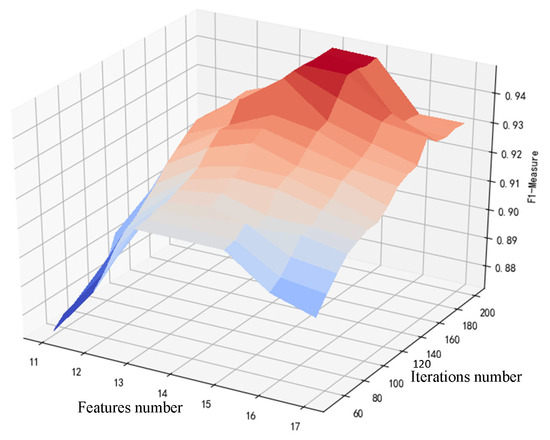
Figure 8.
Tuning results of AdaBoost before optimization.
- Electric traction/brake cannot be applied at the same time as air braking, and the indicator has little effect on air braking.
- When the running line is a bridge, the main factor affecting the decision of air braking is the line slope.
The F1-measure values for the output of different decompression predictions are shown in Table 5. From Table 5, we can see the model has an average F1-measure value of only 0.9502, which does not meet the expected performance.
Table 5.
AdaBoost performance before optimization.
6.2. Optimization Simulation Results
The AdaBoost algorithm was optimized above by adjusting the training methods for sample creation and adjusting the voting weight of the underlying classifier. The optimized model performance validation results are shown in Figure 9.
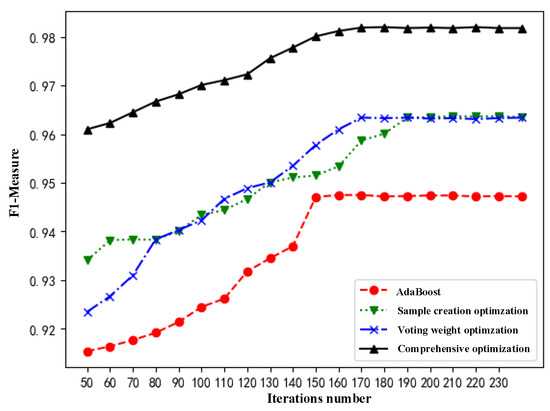
Figure 9.
Comparison of AdaBoost model optimization results.
As can be seen from Figure 9, after only changing the voting weight of the basic weight, the performance of the model has been greatly improved, but the stability period is later. When the number of iterations is small, the change in the number of basic classifiers will have a greater impact on the classification effect; after only adjusting the training subset, the performance of the model will also increase, but the rising speed is slower and the stabilizer is relatively late. With comprehensive optimization after the two algorithms, the performance of the model is significantly improved, the speed is stable, and the optimal number of iterations is 180.
The F1-measure value of the predicted results is shown in Table 6.
Table 6.
Optimized AdaBoost performance.
6.3. Algorithm Simulation Verification
To verify the performance of the model, a set of unused data in the data set is selected as the verification set, and the following evaluations are made on the train operation results.
6.3.1. Security
Comparing the actual driving curve between Shenchi South Station and Suning North Station with the simulation curve, the result is shown in Figure 10. The simulation running speed did not exceed the speed limit curve during the whole journey, and there was no stopping phenomenon, which guaranteed the safety of train operation.
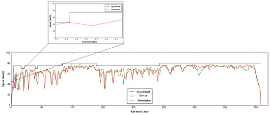
Figure 10.
Comparison of simulation results and driving results.
In Figure 10, the position where the speed limit protection is triggered during the simulation process is partially enlarged, and the whole line is triggered once, and the train is safely protected. It can be seen that the trains correct the abnormal situation in time after the trigger, and the trains can continue to run through emergency braking and alleviating braking.
In addition, we verify the performance of the model in dealing with temporary speed limits by modifying the line speed limit. When the train travels to the 250 km mark, the speed limit of 300 km/h is changed from 80 km/h to 45 km/h. The result is shown in Figure 11, and we can see that the model responds well to the temporary speed limit and improves the efficiency of the train operation. Figure 12 compares the prediction of the model on the Shenchi South Station to the Sanji Station line with the results of the actual output of the driver. As can be seen from the figure, because the driver does not output the brake and the model has a small probability of discrete prediction of the braking situation, the wrong brake will be immediately removed in the next control cycle, which will not cause problems for the safety of the train. When the driver outputs air braking, the model also predicts output braking, only if the output values are different, and this error is within a reasonable range.
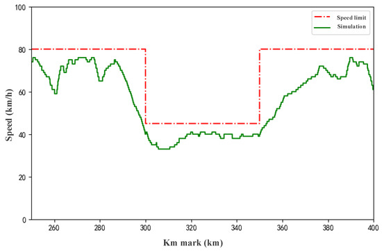
Figure 11.
The v-s curve under temporary speed limit.
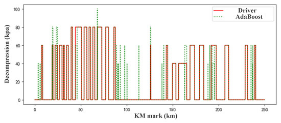
Figure 12.
Comparison of the air brake output.
6.3.2. Air Braking Effectiveness
The line conditions of the ShuoHuang Railway are very complex, including many continuously growing downhill ramps. If the air brake is applied at the wrong time, it will make the cylinder pressure of the train sub-cylinder insufficient and the air brake ineffective.
By comparing the driving of the driver with the speed-distance curve of the model simulation in Figure 13, we can know that between 8 and 40 km, both of them output three air brakes, as indicated by brake recording in Table 7; the model simulation has a braking speed of 60–70 km/h. The mitigation speed is 28 km/h, and the braking charge time is 300–600 s, which meets the safety of brake requirements.
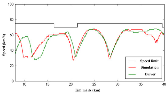
Figure 13.
Comparison of v-s on continuous growth downhill.
Table 7.
Record of the cycle braking on the long downhill.
7. Conclusions
This paper introduces the classification ideas in machine learning into the intelligent control of the air brake of heavy-haul trains, collects the operation data of heavy-haul trains in different formations of the Shuohuang Railway, and introduces a random forest algorithm to evaluate the characteristics of the train operation data. The AdaBoost algorithm is used to model the intelligent control of the air brake of the heavy-haul trains with the CART decision tree as the base classifier, and the AdaBoost algorithm is optimized by improving the generation method of the training subset and the voting weight.
In order to verify the feasibility of the intelligent control model, Shenchi South Station to Suning North Station is selected as the verification interval. By comparing the control results of the intelligent control model with the speed limit information, it is verified that the trains will not stop halfway, and the trains are guaranteed to run at a safe speed. By comparing the intelligent control model with the average driving speed and running time of the driver, the punctuality of the model is verified by using the punctuality index. By comparing the output of the intelligent control model and the air brake driven by the driver on the long downhill, it is confirmed that the two have similar cyclic brake output results, and the recharge time meets the minimum requirements for safe driving.
In short, the feasibility of the algorithm is confirmed from the above indicators, and it is proved that it can ensure the safe and stable operation of trains after being applied to the intelligent driving process of heavy-haul trains.
Author Contributions
Conceptualization, S.W. and L.Z.; methodology, L.Z.; validation, L.C.; formal analysis, S.W. and L.C.; investigation, Q.L.; data curation, S.W. and Q.L.; writing—original draft preparation, S.W.; writing—review and editing, L.Z., L.C. and Q.L. All authors have read and agreed to published version of the manuscript.
Funding
National Key R&D Program of China: 2018YFB1201500; Beijing Natural Science Foundation: L201004, L201002; Fundamental Research Funds for the Central Universities: 2020JBZD002, 2018JBM076, 2021YJS201, 2021CZ107; Natural Science Foundation of China under Grants: 61973026; Beijing Municipal Education Commission Funding I20H100010, I19H100010; Project: RCS2021ZZ005.
Conflicts of Interest
The authors declare no conflict of interest.
References
- Huang, Y.; Tan, L.; Chen, L.; Tang, T. A neural network driving curve generation method for the heavy-haul train. Adv. Mech. Eng. 2016, 8, 1687814016647883. [Google Scholar] [CrossRef]
- Wang, X.; Tang, T.; He, H. Optimal control of heavy haul train based on approximate dynamic programming. Adv. Mech. Eng. 2017, 9, 1687814017698110. [Google Scholar] [CrossRef]
- Wang, X.; Li, S.; Tang, T.; Wang, X.; Xun, J. Intelligent operation of heavy haul train with data imbalance: A machine learning method. Knowl.-Based Syst. 2019, 163, 36–50. [Google Scholar] [CrossRef]
- Chen, R.W.; Li, L.; Zhu, C.Q. Automatic train operation and its control algorithm based on CBTC. J. Comput. Appl. 2007, 27, 2649–2651. [Google Scholar]
- Gruber, P.; Bayoumi, M.M. Suboptimal Control Strategies for Multilocomotive Powered Trains. IEEE Trans. Autom. Control. 1982, 27, 536–546. [Google Scholar] [CrossRef]
- Jin, S.; Hou, Z.; Chi, R. Optimal Terminal Iterative Learning Control for the Automatic Train Stop System. Asian J. Control 2015, 17, 1992–1999. [Google Scholar] [CrossRef]
- Chang, C.S.; Sim, S.S. Optimising train movements through coast control using genetic algorithms. IEEE Proc. Part B 1997, 144, 65–73. [Google Scholar] [CrossRef]
- Bonissone, P.; Khedkar, P.S.; Chen, Y. Genetic algorithms for automated tuning of fuzzy controllers: A transportation application. In Proceedings of the IEEE 5th International Fuzzy Systems, New Orleans, LA, USA, 11 September 1996. [Google Scholar]
- Sekine, S.; Imasaki, N.; Endo, T. Application of fuzzy neural network control to automatic train operation and tuning of its control rules. In Proceedings of the 1995 IEEE International Conference on IEEE, Yokohama, Japan, 20–24 March 1995. [Google Scholar]
- Bai, Y.; Mao, B.; Ho, T.; Feng, Y.; Chen, S. Station Stopping of Freight Trains with Pneumatic Braking. Math. Probl. Eng. 2014, 2014, 1–7. [Google Scholar] [CrossRef]
- Yin, J.; Chen, D.; Li, L. Intelligent Train Operation Algorithms for Subway by Expert System and Reinforcement Learning. IEEE Trans. Intell. Transp. Syst. 2014, 15, 2561–2571. [Google Scholar] [CrossRef]
- Zhu, L.; He, Y.; Yu, F.R.; Ning, B.; Tang, T.; Zhao, N. Communication-based train control system performance optimization using deep reinforcement learning. IEEE Trans. Veh. Technol. 2017, 66, 10702–10717. [Google Scholar] [CrossRef]
- Chen, D.; Chen, R.; Li, Y.; Tang, T. Online learning algorithms for train automatic stop control using precise location data of balises. IEEE Trans. Intell. Transp. Syst. 2013, 14, 1526–1535. [Google Scholar] [CrossRef]
- Hornik, K.; Stinchcombe, M.; White, H. Multilayer feedforward networks are universal approximators. Neural Netw. 1989, 2, 359–366. [Google Scholar] [CrossRef]
- Hua, G.; Zhu, L.; Wu, J.; Shen, C.; Zhou, L.; Lin, Q. Blockchain-Based Federated Learning for Intelligent Control in Heavy Haul Railway. IEEE Access 2020, 8, 176830–176839. [Google Scholar] [CrossRef]
- Su, S.; Wang, X.; Cao, Y.; Yin, J. An Energy-Efficient Train Operation Approach by Integrating the Metro Timetabling and Eco-Driving. IEEE Trans. Intell. Transp. Syst. 2019, 21, 4252–4268. [Google Scholar] [CrossRef]
- Su, S.; Tang, T.; Xun, J.; Cao, F.; Wang, Y. Design of Running Grades for Energy-Efficient Train Regulation: A Case Study for Beijing Yizhuang Line. IEEE Intell. Transp. Syst. Mag. 2019, 13, 189–200. [Google Scholar] [CrossRef]
- Rodriguez-Galiano, V.F.; Ghimire, B.; Rogan, J.; Chica-Olmo, M.; Rigol-Sanchez, J.P. An assessment of the effectiveness of a random forest classifier for land-cover classification. Isprs J. Photogramm. Remote Sens. 2012, 67, 93–104. [Google Scholar] [CrossRef]
- Seo, B.; Kang, S.; Choi, J.; Cha, J.; Won, Y.; Yoon, S. IO Workload Characterization Revisited: A Data-Mining Approach. IEEE Trans. Comput. 2014, 63, 3026–3038. [Google Scholar] [CrossRef]
- Zhang, Y.; Ren, X.; Zhang, J. Intrusion detection method based on information gain and ReliefF feature selection. In Proceedings of the 2019 International Joint Conference on Neural Networks (IJCNN) IEEE, Budapest, Hungary, 14–19 July 2019. [Google Scholar]
- Kaihara, M. Forest Learning Method for Chemical Education. J. Comput. Aided Chem. 2010, 11, 1–10. [Google Scholar] [CrossRef][Green Version]
- Deng, H.; Runger, G.; Tuv, E.; Vladimir, M. A Time Series Forest for Classification and Feature Extraction. Inf. Sci. 2013, 239, 142–153. [Google Scholar] [CrossRef]
- Xu, H.; Zhang, H.; Xu, J.; Wang, G.; Nie, Y.; Zhang, H. Individual Identification of Electronic Equipment Based on Electromagnetic Fingerprint Characteristics. In Proceedings of the 2019 IEEE 6th International Symposium on Electromagnetic Compatibility (ISEMC) IEEE, Nanjing, China, 1–4 November 2019. [Google Scholar]
- Landesa-Vázquez, I.; Alba-Castro, J.L. Double-Base Asymmetric AdaBoost. Neurocomputing 2013, 118, 101–114. [Google Scholar] [CrossRef]
- Denison, D.; Smith, M.A.F. A Bayesian CART algorithm. Biometrika 1998, 85, 363–377. [Google Scholar] [CrossRef]
- Boerstler, H.; Figueiredo, J.M.D. Prediction of use of psychiatric services: Application of the CART algorithm. J. Ment. Health Adm. 1991, 18, 27–34. [Google Scholar] [CrossRef]
- Tang, H.; Wang, Y.; Liu, X.; Feng, X. Reinforcement learning approach for optimal control of multiple electric locomotives in a heavy-haul freight train: A Double-Switch-Q-network architecture. Knowl.-Based Syst. 2019, 190, 105173. [Google Scholar] [CrossRef]
- Liang, H.; Zhang, Y. Research on Automatic Train Operation Performance Optimization of High Speed Railway Based on Asynchronous Advantage Actor-Critic. In Proceedings of the 2020 Chinese Automation Congress (CAC), Shanghai, China, 6–8 November 2020. [Google Scholar]
- Liu, H.; Tian, H.Q.; Li, Y.F.; Zhang, L. Comparison of four Adaboost algorithm based artificial neural networks in wind speed predictions. Energy Convers. Manag. 2015, 92, 67–81. [Google Scholar] [CrossRef]
- Zhu, H.; Koga, T. Face detection based on AdaBoost algorithm with Local AutoCorrelation image. IEICE Electron. Express 2010, 7, 1125–1131. [Google Scholar] [CrossRef][Green Version]


Publisher’s Note: MDPI stays neutral with regard to jurisdictional claims in published maps and institutional affiliations. |
© 2021 by the authors. Licensee MDPI, Basel, Switzerland. This article is an open access article distributed under the terms and conditions of the Creative Commons Attribution (CC BY) license (https://creativecommons.org/licenses/by/4.0/).