
Active Exploration for Obstacle Detection on a Mobile Humanoid Robot

 ,
,
Abstract
:1. Introduction
- We propose a method for an efficient active exploration of the environment to overcome the limitations of sensors with small FOV;
2. Related Work
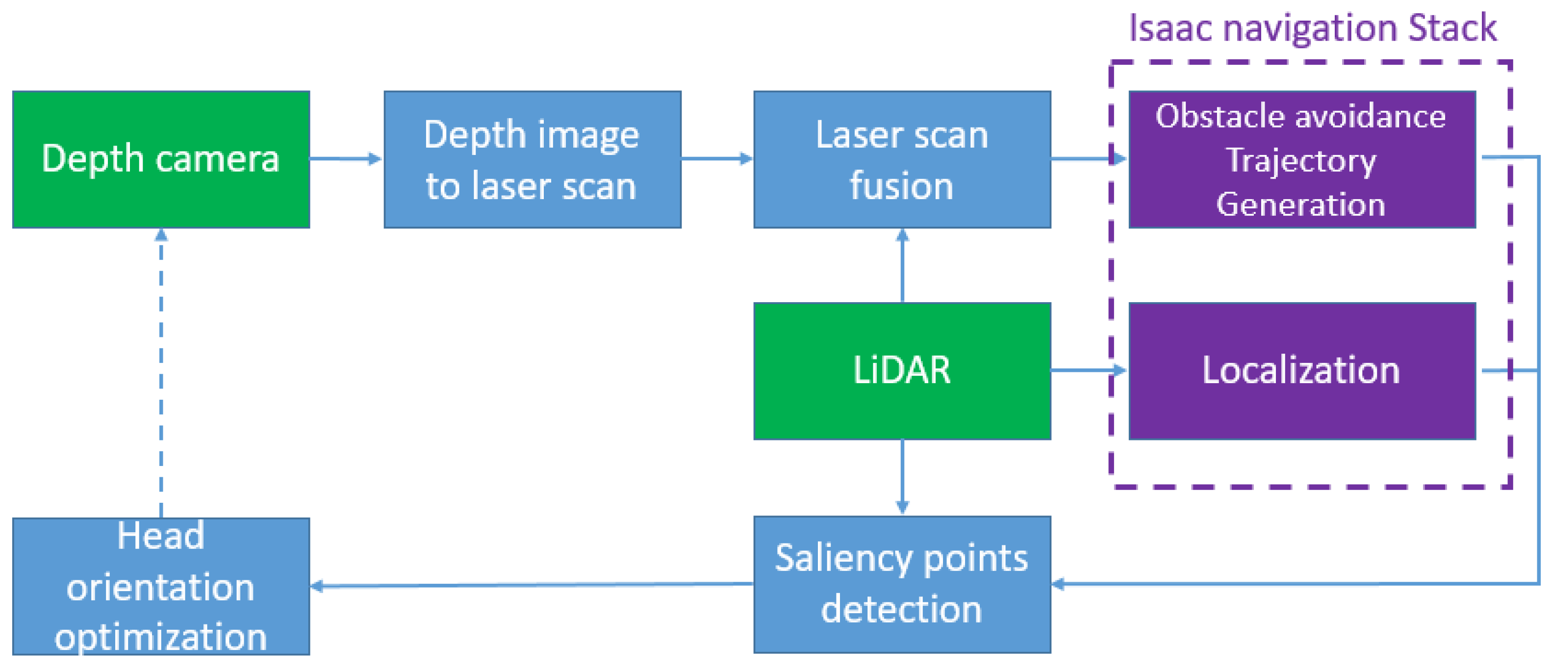
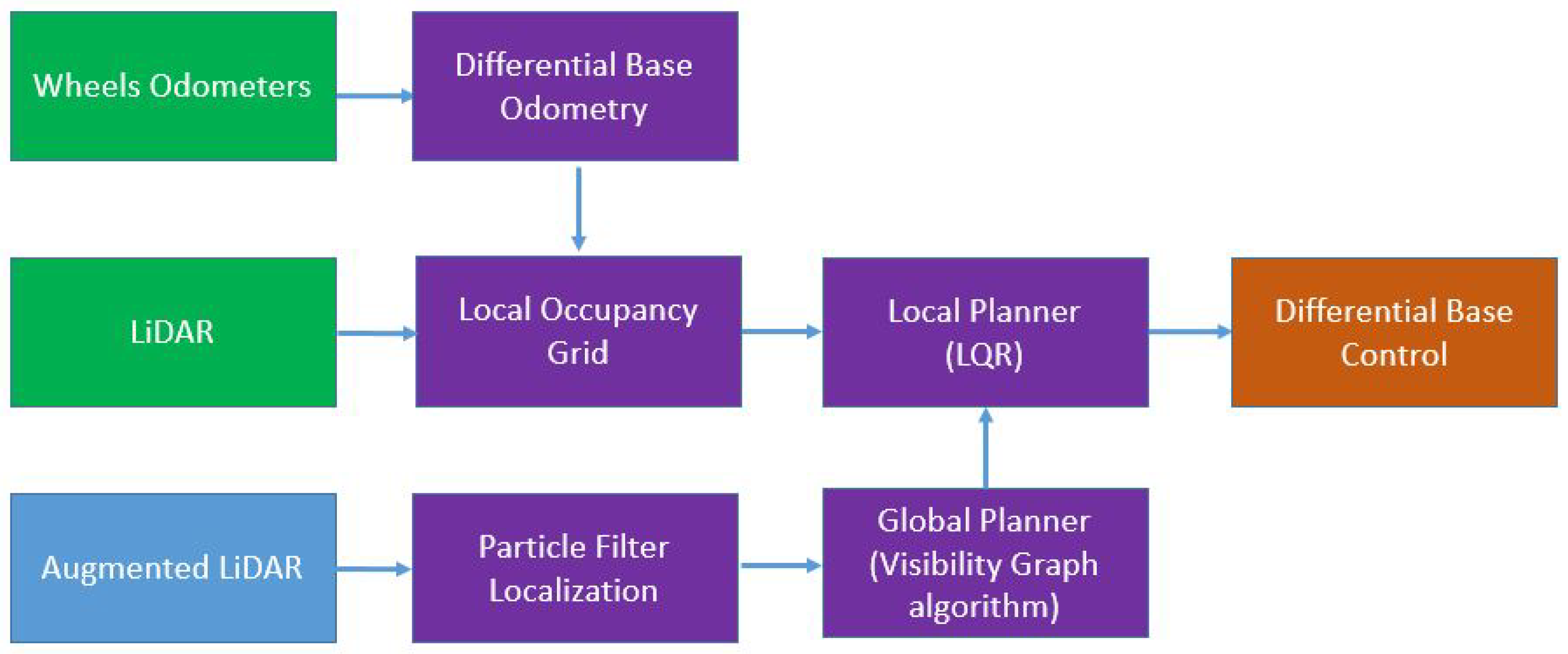
3. Methodology
3.1. Depth Image to 2D Laser Scan
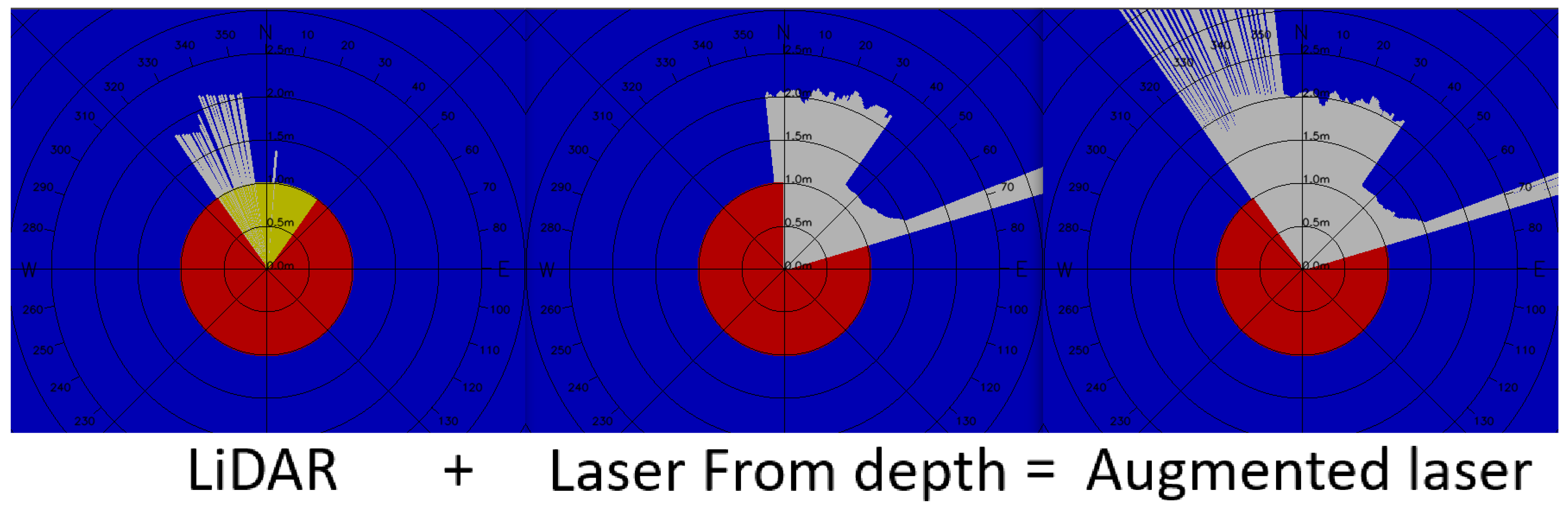
3.2. Laser Scan Fusion
3.3. Nvidia Isaac Navigation
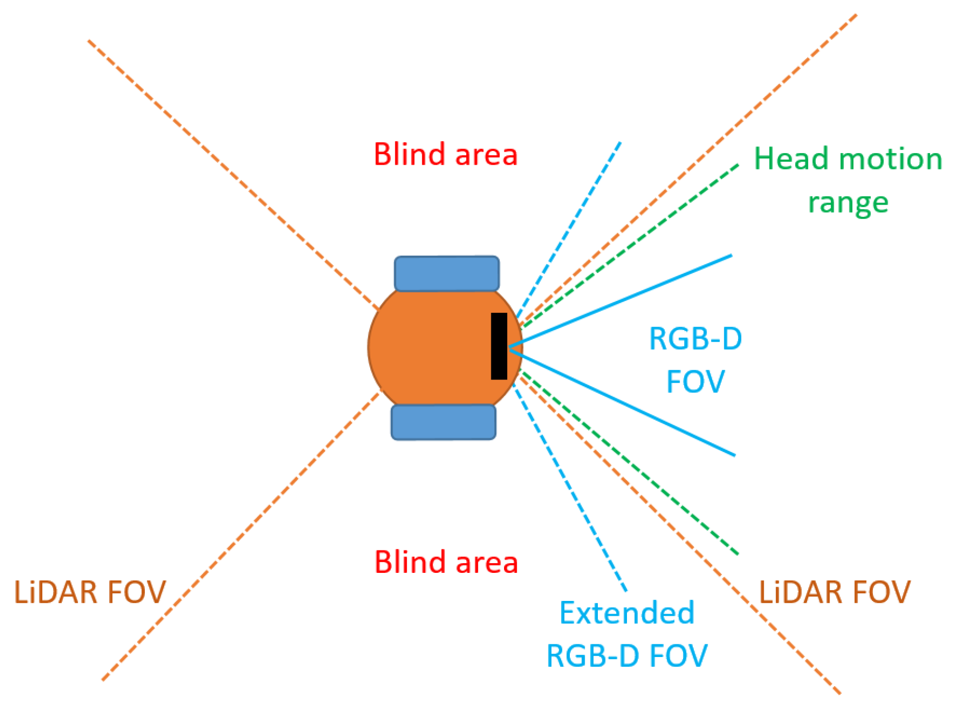
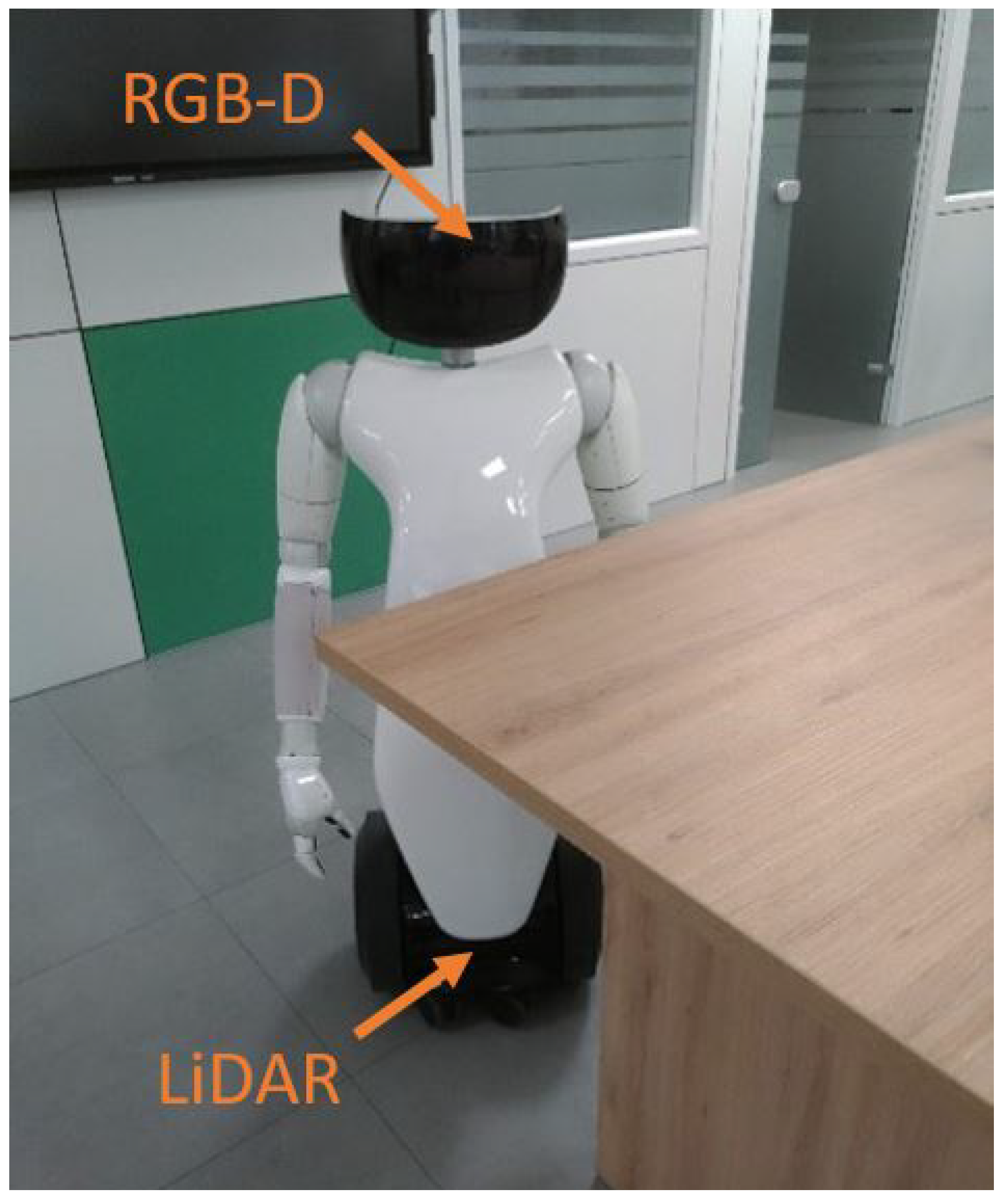
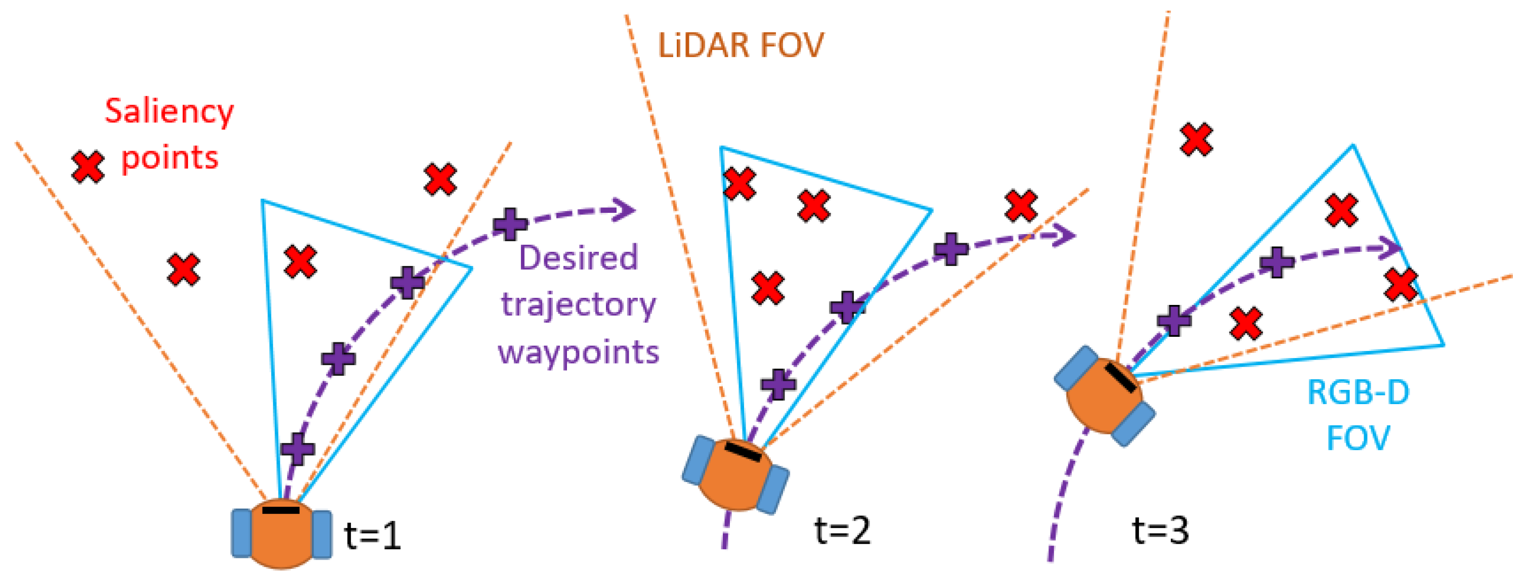
3.4. RGB-D Camera Heading Direction
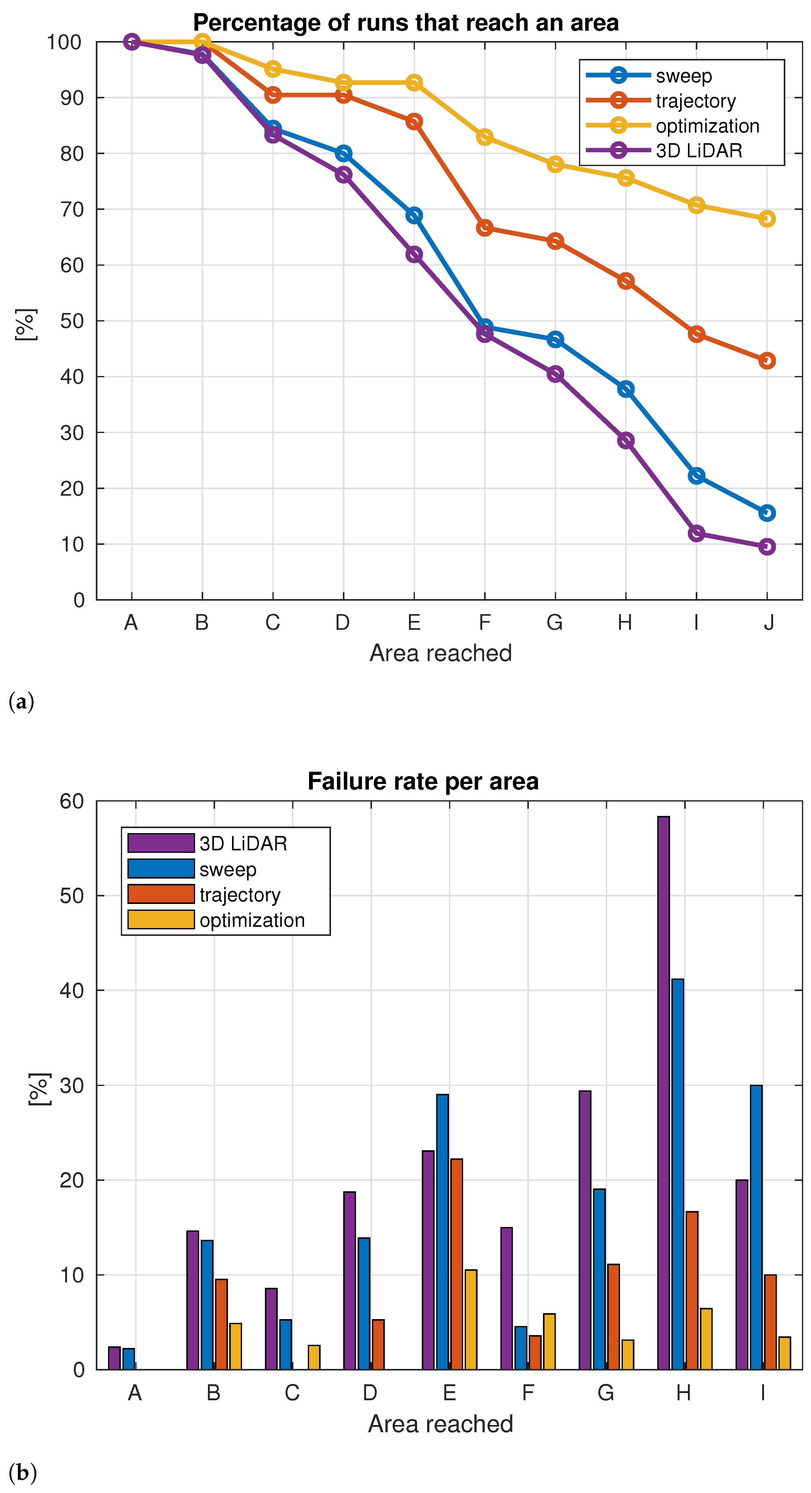
- Sweep: the robot simply moves its head towards the left and right according to the joint limits and given a certain pre-defined maximum speed. This strategy is used as baseline test to evaluate effective improvements achieved with the proposed methods;
- Trajectory: the robot anticipates the global trajectory (i.e., it looks at the intersection point between the global trajectory and a circle centered in the robot with a ±2 m radius);
- Optimized heading (our contribution): at each time step we calculate the optimal head’s heading direction accounting for the future robot’s global trajectory, obstacle candidates points, head turning speed and joints limits of the robot.
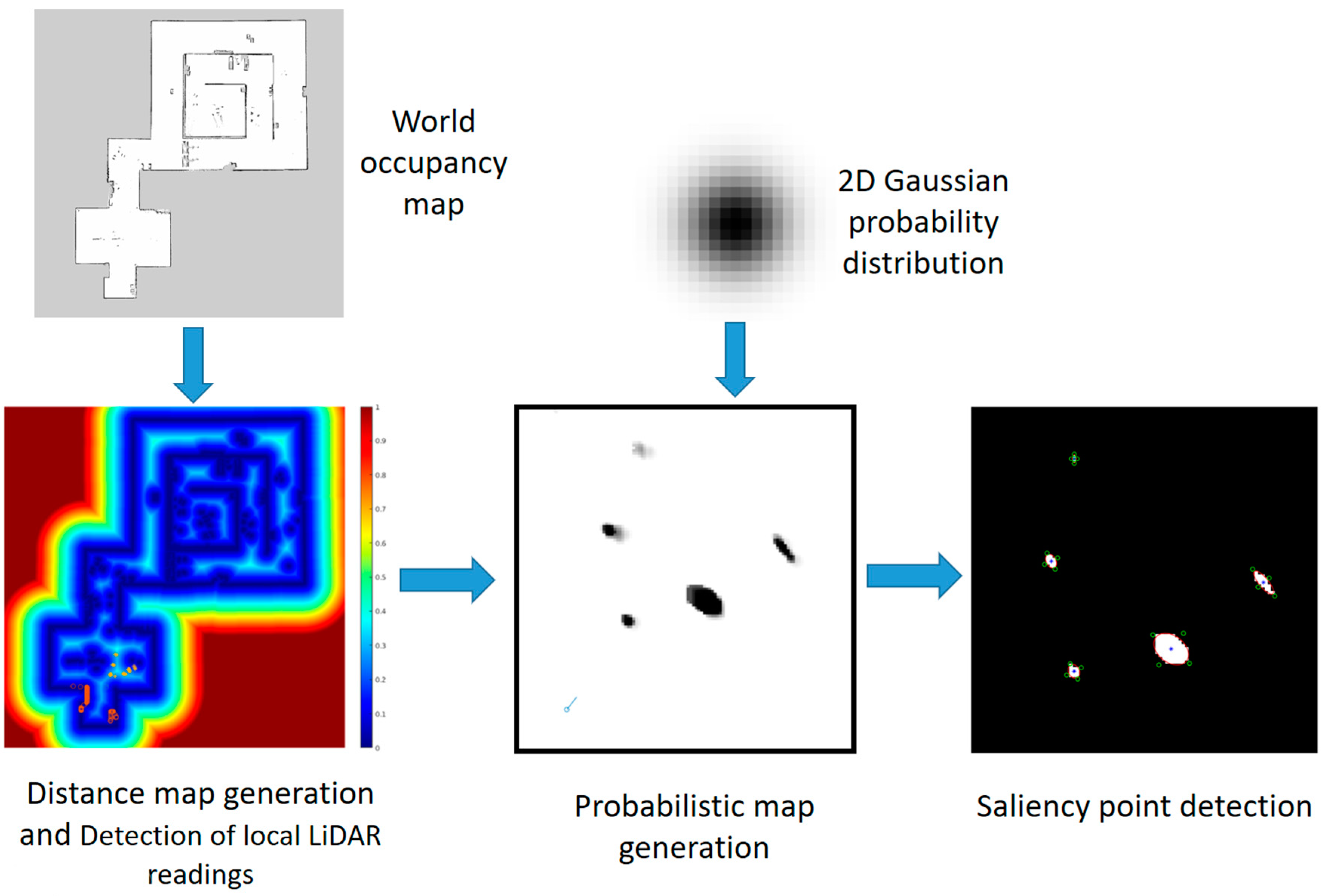
3.5. Salient Point Detector
- The corresponding LiDAR reading must be uncertain and weak;
- The detected point must be local and must not belong to the global map (i.e., it has to be far from walls and other fixed obstacles).
3.6. Head Orientation Optimization
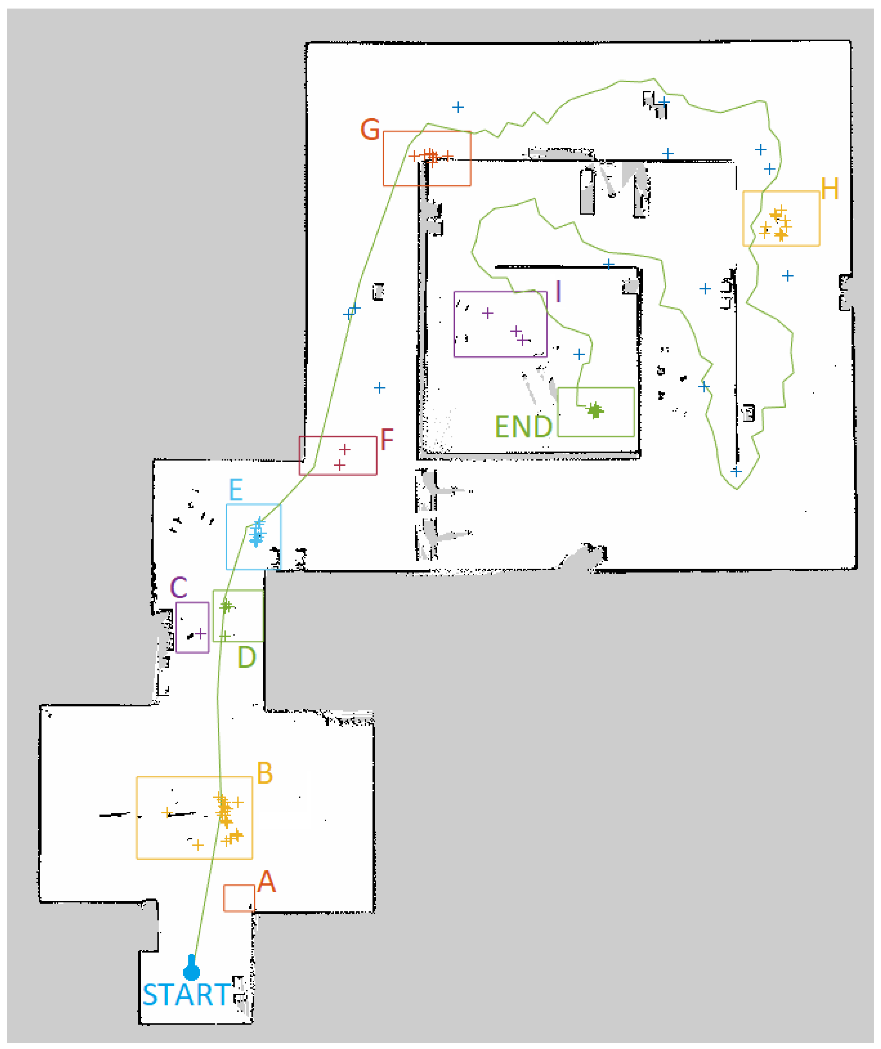
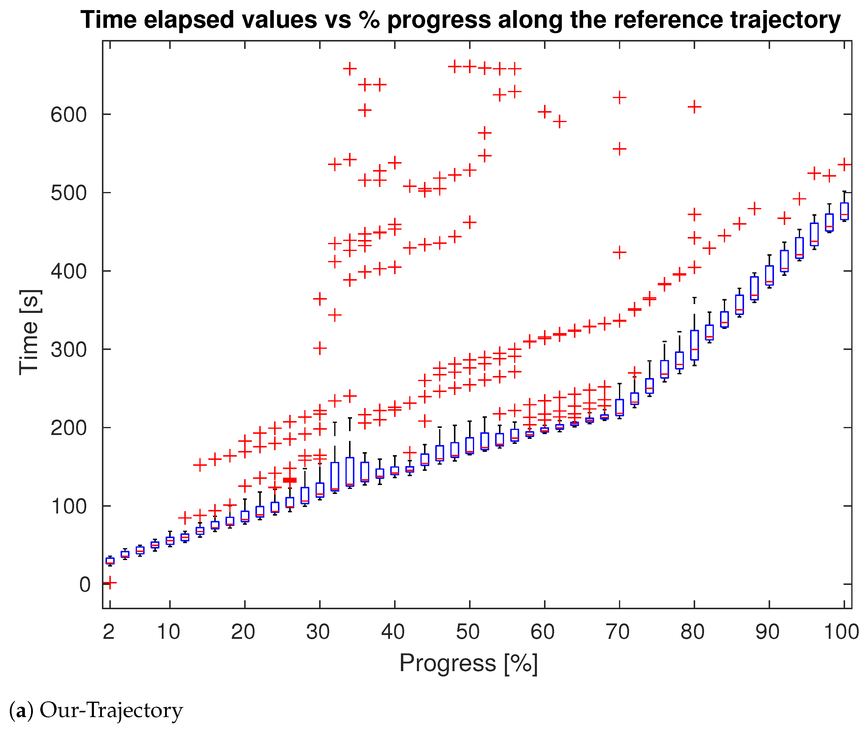
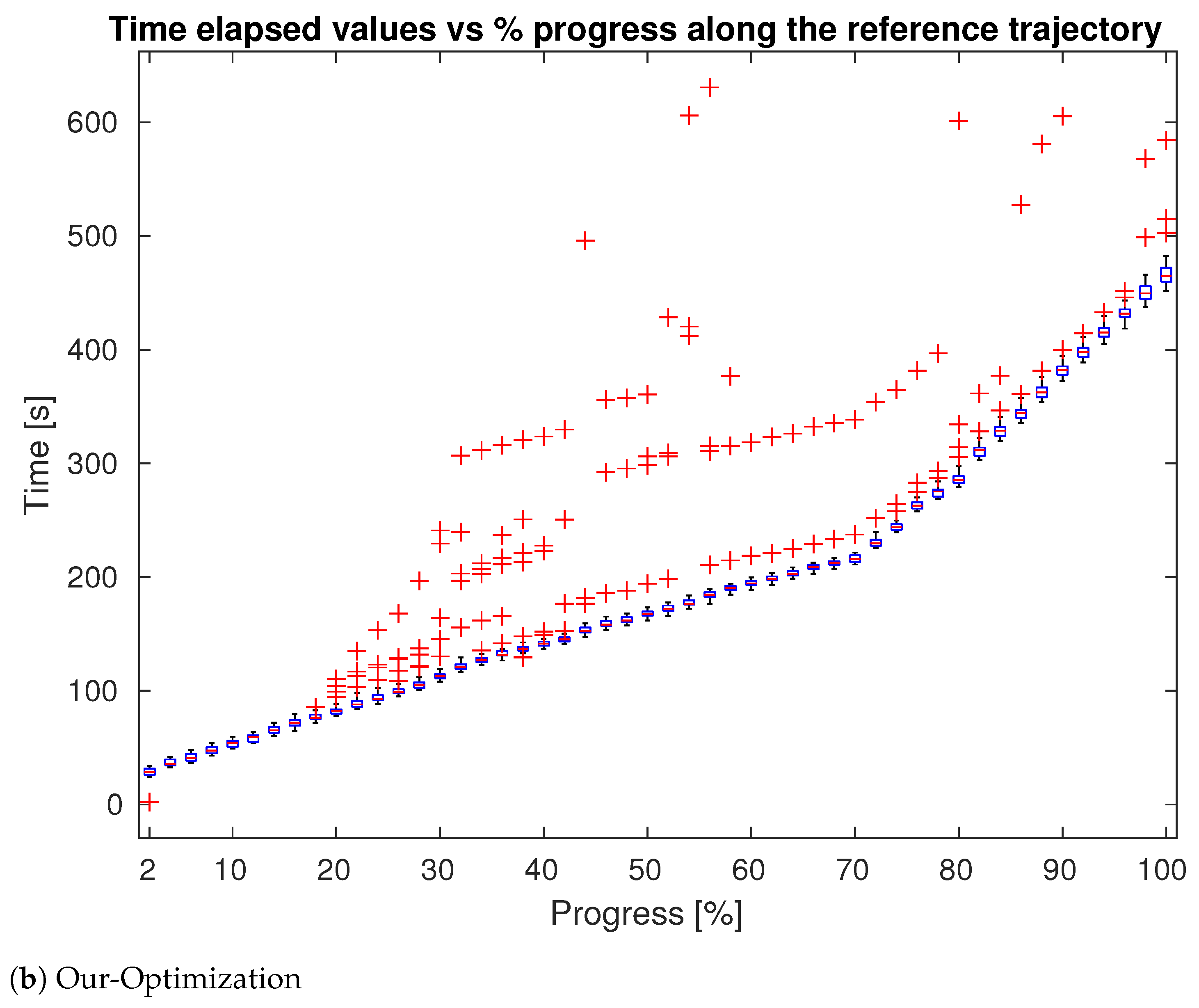
4. Evaluation
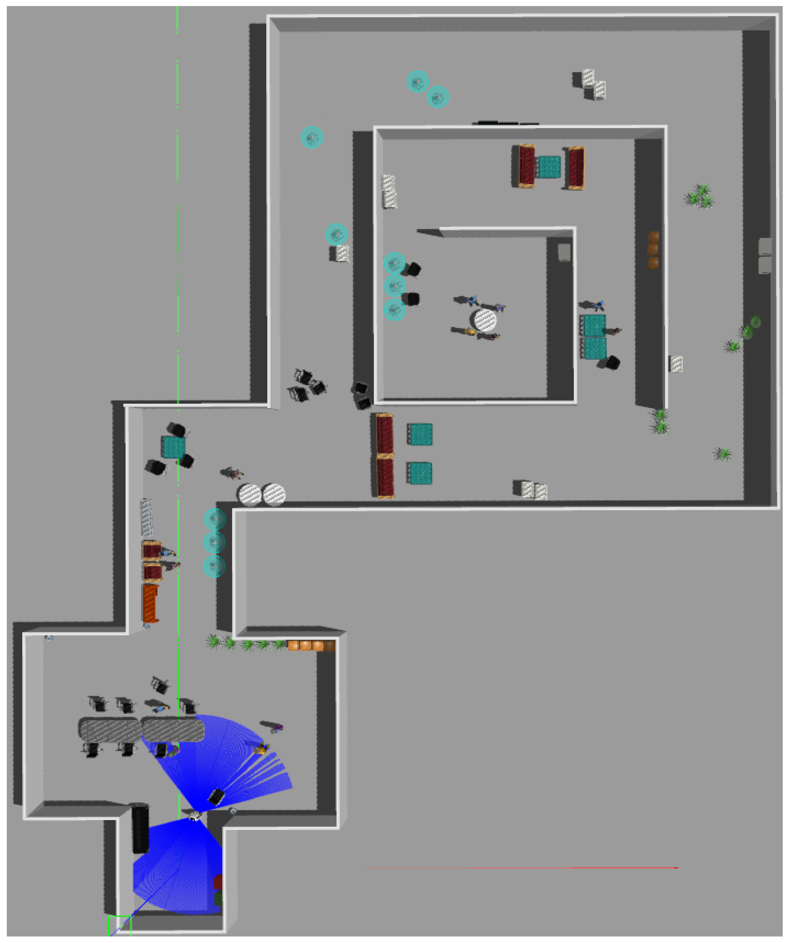
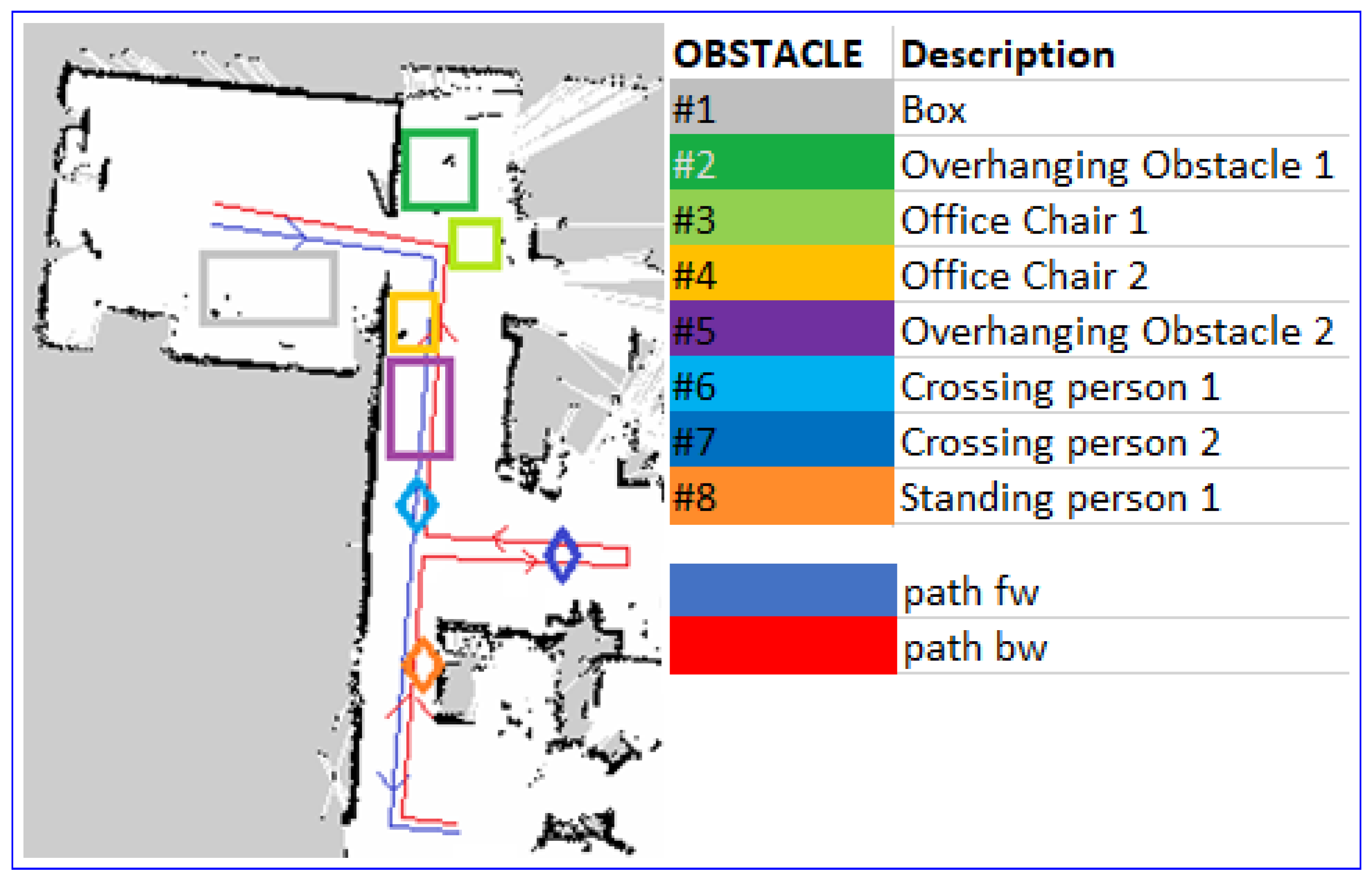
4.1. Tests in Simulation
4.2. Test in Real World
5. Conclusions
Author Contributions
Funding
Institutional Review Board Statement
Informed Consent Statement
Data Availability Statement
Acknowledgments
Conflicts of Interest
References
- Pandey, D.A. Mobile Robot Navigation and Obstacle Avoidance Techniques: A Review. Int. Robot. Autom. J. 2017, 2, 1–12. [Google Scholar] [CrossRef] [Green Version]
- Hassan, S.; Hicks, J.; Lei, H.; Turano, K. What is the minimum field of view required for efficient navigation? Vis. Res. 2007, 47, 2115–2123. [Google Scholar] [CrossRef] [PubMed] [Green Version]
- Bouraine, S.; Fraichard, T.; Salhi, H. Provably safe navigation for mobile robots with limited field-of-views in unknown dynamic environments. In Proceedings of the 2012 IEEE International Conference on Robotics and Automation, Saint Paul, MN, USA, 14–18 May 2012; pp. 174–179. [Google Scholar] [CrossRef] [Green Version]
- Roelofsen, S.; Gillet, D.; Martinoli, A. Collision avoidance with limited field of view sensing: A velocity obstacle approach. In Proceedings of the 2017 IEEE International Conference on Robotics and Automation (ICRA), Singapore, 29 May–3 June 2017; pp. 1922–1927. [Google Scholar] [CrossRef] [Green Version]
- Lopez, B.T.; How, J.P. Aggressive collision avoidance with limited field-of-view sensing. In Proceedings of the 2017 IEEE/RSJ International Conference on Intelligent Robots and Systems (IROS), Vancouver, BC, Canada, 24–28 September 2017; pp. 1358–1365. [Google Scholar] [CrossRef]
- Jain, S.; Malhotra, I. A Review on Obstacle Avoidance Techniques for Self-Driving Vehicle. Int. J. Adv. Sci. Technol. 2020, 29, 5159–5167. [Google Scholar]
- Patle, B.; Babu, L.G.; Pandey, A.; Parhi, D.; Jagadeesh, A. A review: On path planning strategies for navigation of mobile robot. Def. Technol. 2019, 15, 582–606. [Google Scholar] [CrossRef]
- Discant, A.; Rogozan, A.; Rusu, C.; Bensrhair, A. Sensors for Obstacle Detection-A Survey. In Proceedings of the 2007 30th International Spring Seminar on Electronics Technology (ISSE), Cluj-Napoca, Romania, 9–13 May 2007; pp. 100–105. [Google Scholar] [CrossRef]
- Bhattacharya, P.; Gavrilova, M.L. Voronoi diagram in optimal path planning. In Proceedings of the 4th International Symposium on Voronoi Diagrams in Science and Engineering (ISVD 2007), Glamorgan, UK, 9–11 July 2007; pp. 38–47. [Google Scholar] [CrossRef]
- Esan, O.; Du, S.; Lodewyk, B. Review on Autonomous Indoor Wheel Mobile Robot Navigation Systems. In Proceedings of the 2020 International Conference on Artificial Intelligence, Big Data, Computing and Data Communication Systems (icABCD), Durban, South Africa, 6–7 August 2020; pp. 1–6. [Google Scholar] [CrossRef]
- Ni, J.; Li, X.; Fan, X.; Shen, J. A dynamic risk level based bioinspired neural network approach for robot path planning. In Proceedings of the 2014 World Automation Congress (WAC), Waikoloa, HI, USA, 3–7 August 2014; pp. 829–833. [Google Scholar] [CrossRef]
- Quiñonez, Y.; Ramirez, M.; Lizarraga, C.; Tostado, I.; Bekios, J. Autonomous Robot Navigation Based on Pattern Recognition Techniques and Artificial Neural Networks. In Bioinspired Computation in Artificial Systems; Ferrández Vicente, J.M., Álvarez-Sánchez, J.R., de la Paz López, F., Toledo-Moreo, F.J., Adeli, H., Eds.; Springer International Publishing: Cham, Switzerland, 2015; pp. 320–329. [Google Scholar]
- Pang, C.; Zhong, X.; Hu, H.; Tian, J.; Peng, X.; Zeng, J. Adaptive Obstacle Detection for Mobile Robots in Urban Environments Using Downward-Looking 2D LiDAR. Sensors 2018, 18, 1749. [Google Scholar] [CrossRef] [PubMed] [Green Version]
- Young, J.; Simic, M. LIDAR and Monocular Based Overhanging Obstacle Detection. Procedia Comput. Sci. 2015, 60, 1423–1432. [Google Scholar] [CrossRef] [Green Version]
- Han, J.; Liao, Y.; Zhang, J.; Wang, S.; Li, S. Target Fusion Detection of LiDAR and Camera Based on the Improved YOLO Algorithm. Mathematics 2018, 6, 213. [Google Scholar] [CrossRef] [Green Version]
- Redmon, J.; Divvala, S.; Girshick, R.; Farhadi, A. You Only Look Once: Unified, Real-Time Object Detection. In Proceedings of the 2016 IEEE Conference on Computer Vision and Pattern Recognition (CVPR), Las Vegas, NV, USA, 27–30 June 2016; pp. 779–788. [Google Scholar] [CrossRef] [Green Version]
- Song, H.; Choi, W.S.; Lim, S.; Kim, H.D. Target localization using RGB-D camera and LiDAR sensor fusion for relative navigation. In Proceedings of the CACS 2014-2014 International Automatic Control Conference, Conference Digest, Kaohsiung, Taiwan, 26–28 November 2015; pp. 144–149. [Google Scholar] [CrossRef]
- Thapa, V.; Capoor, S.; Sharma, P.; Mondal, A.K. Obstacle avoidance for mobile robot using RGB-D camera. In Proceedings of the 2017 International Conference on Intelligent Sustainable Systems (ICISS), Palladam, India, 7–8 December 2017; pp. 1082–1087. [Google Scholar] [CrossRef]
- Nardi, F.; Lazaro, M.; Iocchi, L.; Grisetti, G. Generation of Laser-Quality 2D Navigation Maps from RGB-D Sensors. In RoboCup 2018: Robot World Cup XXII; Springer International Publishing: Montreal, QC, Canada, 2018. [Google Scholar]
- Keselman, L.; Woodfill, J.I.; Grunnet-Jepsen, A.; Bhowmik, A. Intel(R) RealSense(TM) Stereoscopic Depth Cameras. In Proceedings of the 2017 IEEE Conference on Computer Vision and Pattern Recognition Workshops (CVPRW), Honolulu, HI, USA, 21–26 July 2017; pp. 1267–1276. [Google Scholar] [CrossRef]
- Zhang, Z. Microsoft Kinect Sensor and Its Effect. IEEE Multimed. 2012, 19, 4–12. [Google Scholar] [CrossRef] [Green Version]
- Välimäki, T.; Ritala, R. Optimizing gaze direction in a visual navigation task. In Proceedings of the 2016 IEEE International Conference on Robotics and Automation (ICRA), Stockholm, Sweden, 16–21 May 2016; pp. 1427–1432. [Google Scholar] [CrossRef] [Green Version]
- Lauri, M.; Ritala, R. Stochastic control for maximizing mutual information in active sensing. In Proceedings of the ICRA 2014 Workshop: Robots in Homes and Industry: Where to Look First? Hong Kong, China, 1 June 2014; pp. 1–6. [Google Scholar]
- NVIDIA Corporation. NVIDIA Isaac SDK. Available online: https://developer.nvidia.com/isaac-sdk (accessed on 19 August 2021).
- Fox, D.; Burgard, W.; Dellaert, F.; Thrun, S. Monte Carlo Localization: Efficient Position Estimation for Mobile Robots. In Proceedings of the Sixteenth National Conference on Artificial Intelligence and Eleventh Conference on Innovative Applications of Artificial Intelligence, Orlando, FL, USA, 18–22 July 1999; pp. 343–349. [Google Scholar]
- Nissoux, C.; Simeon, T.; Laumond, J.P. Visibility based probabilistic roadmaps. In Proceedings of the 1999 IEEE/RSJ International Conference on Intelligent Robots and Systems, Human and Environment Friendly Robots with High Intelligence and Emotional Quotients (Cat. No.99CH36289), Kyongju, Korea, 17–21 October 1999; Volume 3, pp. 1316–1321. [Google Scholar] [CrossRef]
- The MathWorks. Matlab Release 2020.a. Natick, MA, USA. Available online: https://it.mathworks.com/products/new_products/release2020a.html (accessed on 19 August 2021).
- Maurer, C.R.; Rensheng, Q.; Raghavan, V. A linear time algorithm for computing exact Euclidean distance transforms of binary images in arbitrary dimensions. IEEE Trans. Pattern Anal. Mach. Intell. 2003, 25, 265–270. [Google Scholar] [CrossRef]
- Maia, M.H.; Galvão, R.K.H. On the use of mixed-integer linear programming for predictive control with avoidance constraints. Int. J. Robust Nonlinear Control 2009, 19, 822–828. [Google Scholar] [CrossRef]
- Makhorin, A. GLPK (GNU Linear Programming Kit Version 4.32). Available online: https://www.gnu.org/software/glpk/ (accessed on 19 August 2021).
- Zhang, J.; Singh, S. LOAM: Lidar Odometry and Mapping in Real-time. In Robotics: Science and Systems; University of California: Berkeley, CA, USA, 2014; Volume 2. [Google Scholar]
- Koenig, N.; Howard, A. Design and use paradigms for Gazebo, an open-source multi-robot simulator. In Proceedings of the 2004 IEEE/RSJ International Conference on Intelligent Robots and Systems (IROS) (IEEE Cat. No.04CH37566), Sendai, Japan, 28 September–2 October 2004; Volume 3, pp. 2149–2154. [Google Scholar] [CrossRef] [Green Version]
- Rasouli, A.; Tsotsos, J.K. The Effect of Color Space Selection on Detectability and Discriminability of Colored Objects. arXiv 2017, arXiv:1702.05421. [Google Scholar]


| Approach | Delay Points # | Delay Points Avg (s) |
|---|---|---|
| Sweep | 348 | 295.6 |
| Trajectory | 281 | 283.4 |
| Optimization | 130 | 253.2 |
| Obstacle Type | Fixed | Sweep | Trajectory | Optimization |
|---|---|---|---|---|
| All | 19.4% | 15.7% | 8.8% | 6.3% |
| Side | 9.4% | 6.9% | 4.4% | 2.1% |
| On-trajectory | 10.0% | 8.8% | 4.4% | 4.2% |
Publisher’s Note: MDPI stays neutral with regard to jurisdictional claims in published maps and institutional affiliations. |
© 2021 by the authors. Licensee MDPI, Basel, Switzerland. This article is an open access article distributed under the terms and conditions of the Creative Commons Attribution (CC BY) license (https://creativecommons.org/licenses/by/4.0/).
Share and Cite
Nobile, L.; Randazzo, M.; Colledanchise, M.; Monorchio, L.; Villa, W.; Puja, F.; Natale, L. Active Exploration for Obstacle Detection on a Mobile Humanoid Robot. Actuators 2021, 10, 205. https://doi.org/10.3390/act10090205
Nobile L, Randazzo M, Colledanchise M, Monorchio L, Villa W, Puja F, Natale L. Active Exploration for Obstacle Detection on a Mobile Humanoid Robot. Actuators. 2021; 10(9):205. https://doi.org/10.3390/act10090205
Chicago/Turabian StyleNobile, Luca, Marco Randazzo, Michele Colledanchise, Luca Monorchio, Wilson Villa, Francesco Puja, and Lorenzo Natale. 2021. "Active Exploration for Obstacle Detection on a Mobile Humanoid Robot" Actuators 10, no. 9: 205. https://doi.org/10.3390/act10090205