Composite Sliding Mode Control of High Precision Electromechanical Actuator Considering Friction Nonlinearity

Abstract

Friction nonlinearity, which is common in electromechanical actuator (EMA) systems, leads to undesired dynamic responses such as “flat top”, low-speed crawl, which brings challenges to high precision attitude control of flight vehicles. In order to improve the robustness of the actuator control system under friction nonlinearity, and suppress the chattering caused by high gain of sliding mode control (SMC), a composite SMC scheme based on modified extended state observer (MESO) is proposed. Nonlinear MESO is adopted for estimating the nonlinear friction dynamics, unmodeled disturbance, and external real-time load dynamics so as to compensate for their adverse effect. At the same time, in order to improve the robustness of EMA, and reduce the tracking error of the servo system, SMC is adopted to ensure the tracking error convergence in a finite time. The stability of the proposed method is proved, and the effectiveness is verified by simulations.

1. Introduction

For high-precision guided flight, the dynamic performance of EMA plays an important role in the attitude and trajectory control of flight vehicles. However, in the traditional attitude control system, EMA is generally simplified as a rigid model, and the nonlinear factors are ignored, then, the model is simplified into a first-order or second-order ideal linear system with a certain bandwidth, and the subsequent attitude controller design is carried out based on it. However, in real EMA and other electromechanical drive systems, nonlinearities, disturbances, and uncertainties are widespread. These factors may come from inside or outside of the system, such as unmodeled dynamics, parameters time-varying, friction [1], backlash [2,3,4], dead-zone [5,6,7,8,9], load disturbances, etc. Therefore, in high-precision situations, these disturbances should not be ignored. The traditional controller, such as PID, can not meet the technical requirements of the modern flight vehicle under these disturbances.

Friction, which exists extensively in EMA, is the main factor affecting the low-speed tracking performance of servo systems, it can cause position tracking errors and speed distortion [10], limit cycles oscillation (LCO), and so on. In order to improve the tracking performance, a corresponding control method must be undertaken to suppress it. Methods based on models [11,12,13,14] and model-independent [15] methods were proposed by researchers in recent years. Model-based compensation methods rely on the friction model and parameter identification of the model, scholars have proposed a variety of friction models. As the LuGre model can describe the friction’s dynamic and static characteristics more completely. Compensation methods based on the LuGre friction model have been widely researched [15,16,17]. However, the friction nonlinearity of EMA is uncertain, and the parameter identification accuracy is highly dependent on the speed signal’s quality, so real-time parameter identification is not easy to be realized. The compensation method based on model-independent has been widely developed because of its simple control algorithm and good real-time performance. Wang [15] proposed an Active Disturbance Rejection Control method for friction compensation and control, and the Extended State Observer (ESO) was used to estimate the system disturbance. The results show that the method can improve the control accuracy to some extent. However, its performance in high bandwidth has not been verified yet. Sliding Mode Control (SMC) has been widely used due to its strong disturbance rejection capability, insensitivity to parameter changes, simplicity, and easy implementation [18]. However, the discontinuous switching characteristics of traditional SMC in nature will cause chattering, and LCO problems will occur in conventional SMC scheme with switching mechanism in the presence of unmodeled dynamics, especially when the second or higher order unmodeled dynamics exists [19], therefore, it is necessary to improve the controller. Fallaha [19] used the exponential function to design nonlinear reaching law, experiments on the robot arm show the effectiveness of the method in chattering suppression, particularly in steady-state. Shepit [20] proposed a state feedback sliding mode controller to achieve a complex eigen-structure assignment, this can be advantageous in providing maximum flexibility in specifying closed loop dynamics. However, the chatter phenomenon still exists. Difonzo [21] characterizes the attractivity for a co-dimension two discontinuity manifold in piecewise smooth differential systems, where a new parameter is proposed to indicate how the integral curve evolves, sliding or spiraling, but how to use this method to design chattering-free controllers is not discussed. For some complex nonlinear dynamic systems, constructing generalized nonlinear Lyapunov functions to establish system stability might be simpler [22], however, constructing the proper global Lyapunov function would be quite tough.

External disturbances, nonlinearity, and unmodeled disturbances are the main sources of chattering in sliding mode control [23]. Aiming at the friction nonlinearity and disturbance of electromechanical systems, a new adaptive sliding mode control scheme is proposed by Wang [24] based on a neural network to estimate the nonlinear and unmodeled dynamics of friction. The effectiveness is verified, but the real-time performance of the intelligent method is relatively poor in the case of high dynamic response. The ESO is a novel observe algorithm, which is able to estimate internal and external disturbance online [25], Deng [25,26,27] integrates linear ESO into controllers to develop high performance control of the systems with nonlinear dynamics or disturbances and unmeasurable signals, the unmeasured velocity, model uncertainty, mismatched disturbance, and bounded disturbance are estimated by ESO, and the estimated information is used to design the controllers, and the control effect is verified. Ren [28] proposed a friction compensation method based on an ESO, the effectiveness and robustness were verified in compensating for the robot friction effects. Different from robot control, the aircraft steering gear only has a position detection device, and the hinge torque changes in real-time during the flight.

In this paper, the effect of EMA friction nonlinearity on the attitude control system of an axisymmetric flight vehicle is analyzed, and the influence of friction on EMA servo dynamic characteristics and its compensation method are studied. In order to compensate for the nonlinear dynamics of EMA, a composite control strategy based on MESO and SMC is proposed. In this strategy, MESO is used to estimate nonlinear dynamics, load disturbances, and unmodeled dynamics and compensate for them in real-time, and SMC based on reaching law is used to enhance the robustness.

This paper is organized as follows, modeling and analysis of EMA are presented in Section 2, in Section 3, a composite controller based on MESO and SMC is designed for the EMA model, and the convergence of the system is proved. In Section 4, the performance of the proposed controller is compared with traditional SMC and Active Disturbance Rejection Control. Finally, conclusions are drawn in Section 5.

2. Modeling and Analysis of EMA

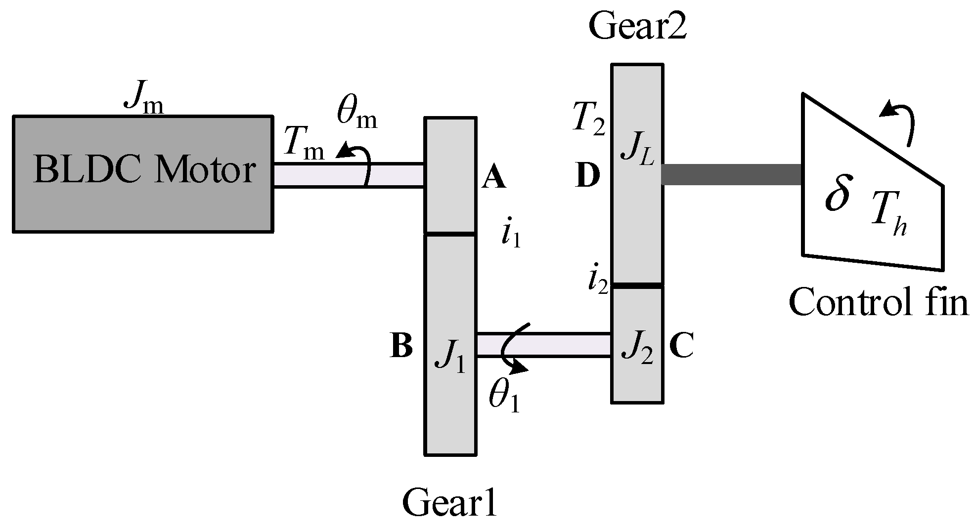
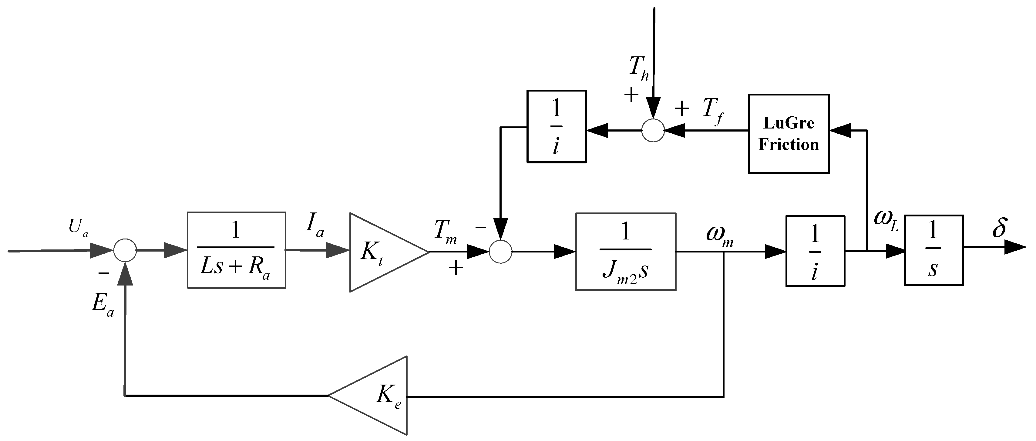
2.1. Modeling of EMA

As shown in Figure 1 [29], the simplified EMA system of the flight vehicle consists of DC brushless servo motor, control surface, drive control device, mechanical transmission mechanism, etc.

In Figure 1, the mechanical transmission section of EMA contains two stages of reducer, $J_m$, $J_1$, $J_2$, $J_L$ are the rotational inertia of the motor, the corresponding gear inertia, and load inertia, respectively. ${\theta }_m$ and ${\theta }_1$ are the output angles of motor and gear 1, $i_1$ and $i_2$ are the transmission ratios of two gears, and $\delta$ is the deflection angle of EMA.

For the brushless DC motor, ignoring viscous damping parameters, The mathematical model of the EMA system without a controller can be written as follows [10]:

The phase voltage equation is

$$U_a(t)=R_a{I}_a(t)+L\frac{d{I}_a(t)}{dt}+E_a(t)$$

(1)

where $U_a(t)$ is the control voltage of the motor, $R_a$ is the winding phase resistance, $I_a(t)$ is phase current, $L$ is equivalent phase winding inductance, and $E_a(t)$ is phase induced electromotive force (EMF).

Phase EMF equation is

$$E_a(t)=K_E{\omega }_m(t)=K_E\frac{d{\theta }_m(t)}{dt}$$

(2)

where ${\omega }_m(t)$ is the angular velocity of the motor, ${\theta }_m(t)$ is the angle of the motor, and $K_E$ is the back-EMF coefficient.

The output electromagnetic torque of the motor is

$$T_m(t)=K_{\mathrm{T}}{I}_{\mathrm{a}}(t)$$

(3)

where $T_m(t)$ is the output electromagnetic torque, and $K_{\mathrm{T}}$ is the torque coefficient.

The torque balance equation of the motor can be written as

$$T_m(t)=J_m\frac{d{\omega }_m(t)}{dt}+T_L$$

(4)

where $T_L$ is the equivalent load torque.

Apply the Laplace transform to Equations (1)–(4), and after ignoring $T_L$, the open-loop transfer function of the motor output angle is obtained

$$G_{U_a}^{{\theta }_m}(s)=\frac{K_t}{K_e{K}_{t}s+J_m(Ls+R_a)s^2}=\frac{1/K_e}{s({\tau }_m{\tau }_e{s}^2+{\tau }_{m}s+1)}$$

(5)

where ${\tau }_m=\frac{J_m{R}_a}{K_e{K}_t}$ is the mechanical time constant, and ${\tau }_e=\frac{L}{R_a}$ is the electrical time constant.

If the elasticity of the mechanical transmission system is neglected, the rotational inertia of the load and gears can be reduced to the motor side, and the total transmission ratio is $i=i_1{i}_2$. Then, the model of EMA can be simplified to be a rigid one.

In order to study the effects of EMA’s friction nonlinearity on flight control, first of all, the friction torque to EMA should be analyzed. It is assumed that the load torque of the EMA includes only including hinge torque $T_h$ and friction torque $T_f$, then $\delta$ and $T_L$ can be represented as

$$\left\{\begin{array}{c}\delta =\frac{{\theta }_m}{i}\\ T_L=\frac{T_h+T_f}{i}\end{array}\right.$$

(6)

The LuGre model [30] is adopted for friction modeling and is expressed as

$$\left\{\begin{array}{l}\frac{dz}{dt}={\omega }_L-\frac{\left|{\omega }_L\right|}{g\left({\omega }_L\right)}z\hfill \\ {\sigma }_{0}g\left({\omega }_L\right)=T_C+\left(T_S-T_C\right){\mathrm{e}}^{-{\left({\omega }_L/{\omega }_s\right)}^2}\hfill \\ T_f=\lambda \left({\sigma }_{0}z+{\sigma }_1\frac{\mathrm{d}z}{ \mathrm{d}t}+{\sigma }_2{\omega }_L\right)\hfill \end{array}\right.$$

(7)

where $z$ is the average deformation of bristles, $T_C$ is coulomb friction torque, $T_{\mathrm{S}}$ is maximum static friction torque, ${\sigma }_0$, ${\sigma }_1$, ${\sigma }_2$ are bristle stiffness coefficient, bristle damping coefficient and viscous friction coefficient, ${\omega }_L=\dot{\delta }$ is the deflection angular velocity of the EMA output, ${\omega }_s$ is the Stribeck velocity and $\lambda$ is the variation coefficient of friction torque [31]. These parameters can be obtained by identification method [32]. From Equations (1)–(7), the model block diagram of EMA can be obtained as in Figure 2.

Based on the diagram and equations, an open-loop model of EMA with friction can be obtained as

$$\ddot{\delta }=a\dot{\delta }+bu+d$$

(8)

where $a=\frac{-Ke{K}_t+{\sigma }_2{R}_a}{J_{m2}{R}_a{i}^2},b=\frac{K_t}{J_{m2}i{R}_a},d=-\frac{T_h+{\sigma }_{0}z+{\sigma }_1\dot{z}}{J_{m2}{i}^2}$, $J_{m2}$ is the equivalent rotating inertia of EMA, $u$ is the control voltage $U_a$. For EMA, $d$ is related to friction, hinge torque, etc., and it is bounded. Parameters related to EMA and friction identification parameters are shown in

Table 1. EMA parameters.

Symbol	Value	Symbol	Value
$i$	315	$K_t$	$0.056(\mathrm{N}\cdot \mathrm{m}/\mathrm{A}$)
$J_m$	$3.6\times {10}^{-6}(\mathrm{kg}\cdot {\mathrm{m}}^2$)	$R_a$	$3.15(\Omega )$
$J_L$	$5.5\times {10}^{-3}(\mathrm{kg}\cdot {\mathrm{m}}^2$)	$U$	$28.0\left(\mathrm{V}\right)$
$K_e$	$0.056(\mathrm{V}/\mathrm{rad}/\mathrm{s}$)	$L$	$3.2(\mathrm{mH}$)
${\sigma }_0$	$7800(\mathrm{N}\cdot \mathrm{m}\cdot {\mathrm{rad}}^{-1}$)	${\sigma }_1$	$37.5(\mathrm{N}\cdot \mathrm{m}\cdot \mathrm{s}\cdot {\mathrm{rad}}^{-1}$)
${\sigma }_2$	$0.3(\mathrm{N}\cdot \mathrm{m}\cdot \mathrm{s}\cdot {\mathrm{rad}}^{-1}$)	${\omega }_s$	$0.063{(}^{\circ }/\mathrm{s})$
$T_C$	$1.4(\mathrm{N}\cdot \mathrm{m}$)	$T_S$	$2.04(\mathrm{N}\cdot \mathrm{m}$)

.

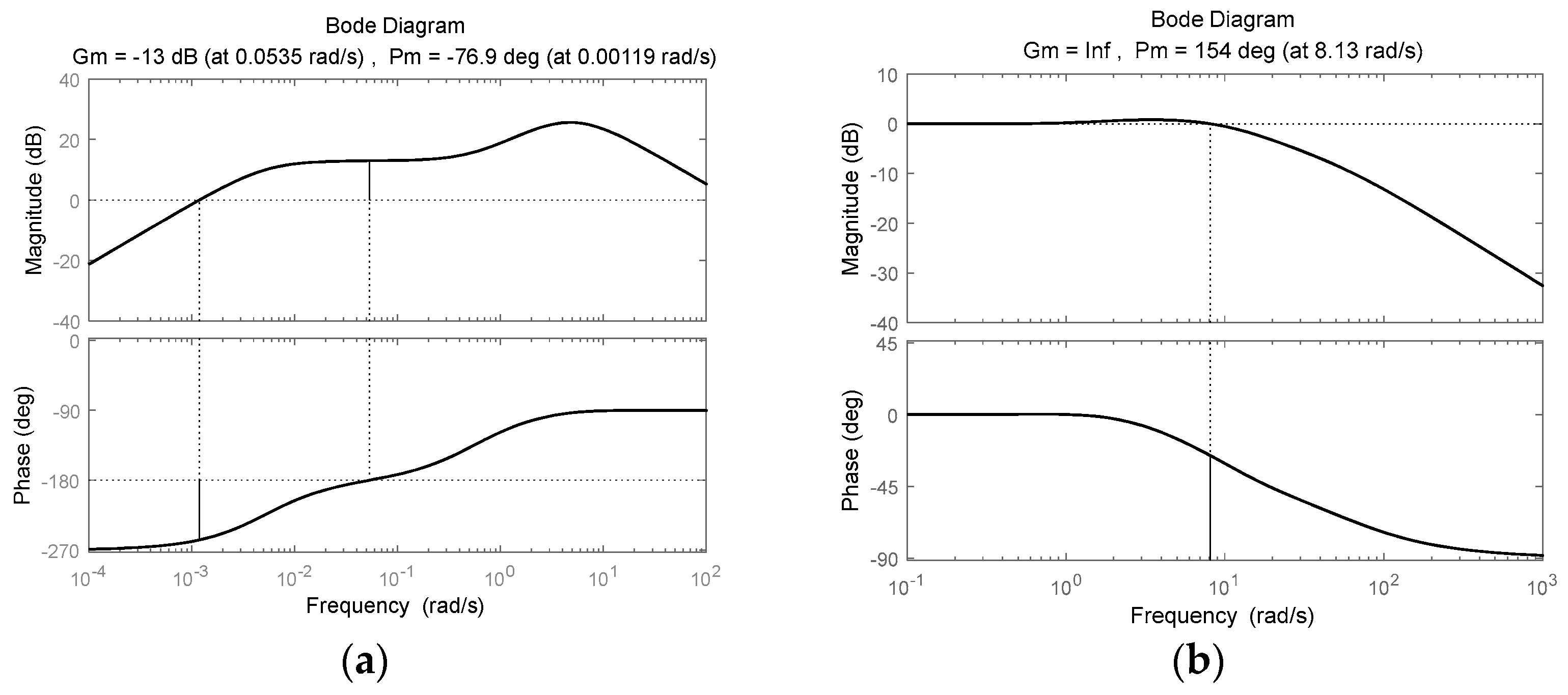
2.2. Influence of Friction Nonlinearity on Attitude Control of Flight Vehicle

In-flight attitude control, EMA is the inner loop, and the attitude control is the outer loop, the nonlinearity of the inner loop will lead to unexpected dynamics.

2.2.1. Friction Nonlinearity Effects on EMA Dynamics under PID Control

For the EMA model, take position error $e_p={\delta }_c-\delta$, PID controller can be described as

$$u=k_p{e}_p+k_i\int e_p+k_d{\dot{e}}_p$$

(9)

where ${\delta }_c$ is the position command value, and $k_p$, $k_i$, $k_d$ are the proportional, integral, and differential coefficients, respectively. Parameters were designed by ITAE criterion [33]: $k_p$ = 33, $k_i$ = 895, $k_d$ = 0.15, take $\lambda$ = 4. Ignoring hinge torque, dynamic responses of position and speed under friction nonlinearity of EMA can be seen in Figure 3 and Figure 4.

The simulation results show that, when the position command is small and the frequency is low, friction nonlinearity of EMA may cause the “flat top” phenomenon of position tracking under PID control, meanwhile, speed curve distortion is generated.

2.2.2. Influence of EMA Friction Nonlinearity on Attitude of Flight Vehicle

• Flight vehicle model and controller design

The flight vehicle in this paper has an axisymmetric cross structure, the length of the body is 4.76 m, the characteristic length is 0.273 m, and the booster time is 8.2 s, and the maximum range is 300 km. During the flight of the vehicle, fuel consumption, flight altitude, speed, trajectory, and other parameters are changed in real-time, flight attitude transfer function model between equivalent actuator to pitch angle is

$$G_{\delta }^{\vartheta }=\frac{a_{25}s+a_{25}\left(a_{34}-a_{33}\right)-a_{35}{a}_{24}}{s^3+\left(a_{34}-a_{33}-a_{22}\right)s^2+\left[a_{22}\left(a_{33}-a_{34}\right)-a_{24}\right]s+a_{33}{a}_{24}}$$

(10)

where $a_{22}=\frac{M_z^{{\omega }_z}}{J_z}$, $a_{24}=\frac{M_z^{\alpha }}{J_z}$, $a_{26}=\frac{1}{J_z}$, $a_{33}=\frac{g\sin \theta }{V}$, $a_{34}=\frac{P+Y^{\alpha }}{mV}$, $a_{35}=\frac{Y^{{\delta }_z}}{mV}$ are corresponding dynamic coefficients, $J_z$ is the moment of inertia, $m$ is the mass of the vehicle at the feature point, $V$ is the velocity vector, $g$ is gravitational acceleration, $\theta$ is trajectory inclination angle, $P$ is thrust, $Y^{\alpha }$ is derivative of lift generated by the angle of attack, $M_z^{\alpha }$, $M_z^{{\omega }_z}$, $M_z^{{\delta }_z}$ are the angle of attack moment coefficient, angular velocity moment coefficient, and actuator moment coefficient, respectively.

Take 10 s after launching as the feature point. At this point, the dynamic pressure is large and the aerodynamic nonlinear factor is strong, it is suitable to study the influence of EMA friction nonlinearity on the attitude of the flight vehicle. First of all, without considering the nonlinearity of EMA, design the PID attitude controller of the feature point. By substituting aerodynamic parameters, the model of the flight vehicle in 10 s is

$$G=\frac{183.8s+102.9}{s^3+0.5668s^2-23.11s+0.1197}$$

(11)

The diagram of the attitude control model is shown in Figure 5.

It is assumed that the EMA has ideal dynamic characteristics, then the PID parameters of the controller can be designed as $k_{pf}$ = 4.54, $k_{if}$ = 6.44, $k_{df}$ = 0.13, $k_w$ = 0.2. Figure 6 shows the open loop and closed loop Bode diagrams of the longitudinal attitude transfer function of the model.

It can be seen from Figure 6a that, at this point, the model is a non-minimum phase system and the system is statically unstable. After compensation, see Figure 6b, the system is stable and the control bandwidth is 18.8 rad/s.

2.

Analysis of EMA friction nonlinearity influence on attitude control

In the presence of friction nonlinearity, the dynamic characteristics of EMA are considered in Figure 5. The influence of EMA friction nonlinearity on attitude control is studied by simulation. The result is shown in Figure 7.

As can be seen from Figure 7, the pitching angle results in unexpected dynamics due to the friction nonlinearity of EMA. With the friction torque increasing, the overshot of the pitch angle response increases slightly, and when $\lambda$ = 8, the dynamic response of the pitch angle appears LCO. Therefore, for high precision flight control, the existence of EMA friction will lead to undesirable attitude dynamic responses under PID control, which is unacceptable. So, it is necessary to compensate for the friction nonlinearity of EMA.

3. Composite SMC Based on MESO

In order to enhance the disturbance suppression and improve its robustness, SMC is often used [10,18,34] to achieve high dynamic performance of EMA. However, conventional SMC methods [35] always contain a discontinuous sign function and large switching gains, so control chattering is unavoidable. External disturbances, nonlinearity, and unmodeled disturbances are the main sources of chattering in sliding mode control [23], ESO is a good way to estimate these disturbances.

In this section, for the EMA system considering friction nonlinearity, in order to eliminate chattering and enhance the robustness, a composite SMC based on MESO is proposed.

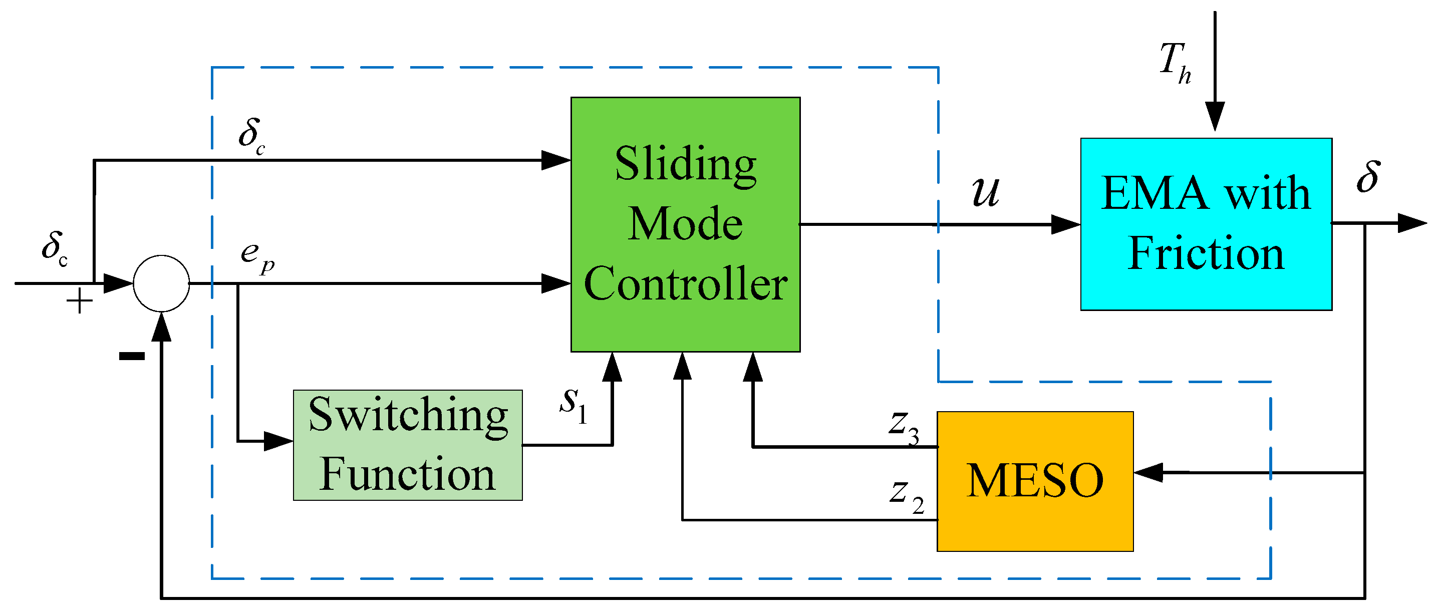
3.1. Design of Composite SMC Based on MESO

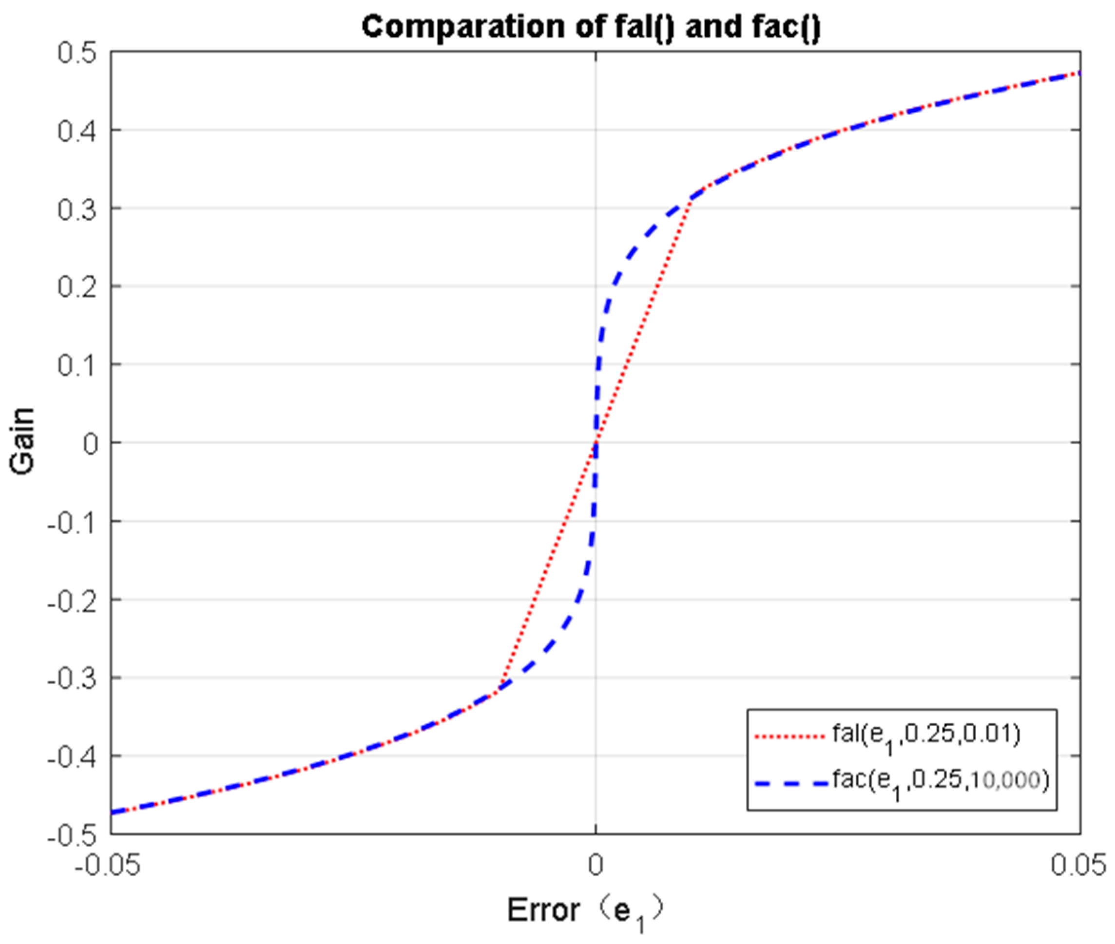
In this section, the proposed composite SMC control strategy based on MESO is introduced in detail. The proposed control diagram can be seen in Figure 8.

3.2. Design of MESO

For the EMA model with friction, as shown in Figure 2 and Equation (8), $T_f$ is friction torque, $T_h$ is load hinge torque, take $x_1=\delta ,x_2=\dot{\delta }$ as state variables, and treating the unknown dynamics, $x_3$ as an expand state, then, expanded EMA model can be rewritten as:

$$\left\{\begin{array}{l}{\dot{x}}_1=x_2\\ {\dot{x}}_2=a{x}_2+d+bu=x_3+bu\\ {\dot{x}}_3=w(t)\\ y=x_1\end{array}\right.$$

(12)

where, $a=\frac{-Ke{K}_t+{\sigma }_2{R}_a}{J_{m2}{R}_a{i}^2}$, $b=\frac{K_t}{J_{m2}i{R}_a}$, $d=-\frac{T_h+{\sigma }_{0}z+{\sigma }_1\dot{z}}{J_{m2}{i}^2}$, $J_{m2}$ is the equivalent rotational inertia of the EMA system. $x_3=a{x}_2+d=f(x_2,d,t)$, that is the overall disturbance including friction nonlinearity which represent the real-time action of acceleration, it is assumed that the first derivative of $x_3$ exits. and $w(t)$ is bounded. Since the LuGre friction model can be linearized around zero, and several dynamic friction models satisfy this assumption, such as the Dahl model, the assumption is reasonable [36].

Because nonlinear ESO can make full use of the characteristics of nonlinear functions to further improve the performance of the observer, nonlinear ESO is a better way to estimate disturbances. The traditional nonlinear state observer of the system (12) is given by

$$\left\{\begin{array}{c}\begin{array}{l}{e}_1=z_1-y\\ {\dot{z}}_1=z_2-{\beta }_1{e}_1\\ {\dot{z}}_2=z_3-{\beta }_{2}fal(e_1,{\alpha }_1,{\delta }_1)+bu\\ {\dot{z}}_3=-{\beta }_{3}fal(e_1,{\alpha }_2,{\delta }_1)\end{array}\end{array}\right.$$

(13)

Equation (13) is ESO designed by Han [37]. It can be seen that ESO is only related to the information of $u$ and $y$, and it’s independent of the disturbance models. In (13), ${\beta }_1$, ${\beta }_2$, ${\beta }_3$ are positive gain coefficients, $0<{\alpha }_i<1,i=1,2$, ${\delta }_1>0$ is the width of the linear interval, and nonlinear error feedback function:

$$fal(e_1,{\alpha }_i,{\delta }_1)=\left\{\begin{array}{ll}{\left|e_1\right|}^{{\alpha }_i}sign(e_1),& \left|e_1\right|>{\delta }_1\\ \frac{\left|e_1\right|}{{\delta }_1{}^{1-{\alpha }_i}},& \left|e_1\right|\le {\delta }_1\end{array}\right.$$

(14)

It has been proven [38] that all states can be tracked well by designing reasonable parameters and ESO can be converged. However, in Equation (14), the nonlinear error feedback function is a piecewise function about $e_1$, at the switching point ${\delta }_1$, there would be a value mutation of $z_2$ and $z_3$, then the disturbance cannot be compensated effectively. To solve this issue, at ${\delta }_1$, differential linearization of the error feedback function is adopted. Taking the first quadrant as an example, from Equation (14), we can obtain

$${\left.fal(e_1,a_i,{\delta }_1)\right|}_{e_1^{\ast }}=\left\{\begin{array}{ll}{a}_i{e}_1^{a_i},& e_1>{\delta }_1\\ {\delta }_1{}^{a_i-1}{e}_1,& 0<e_1\le {\delta }_1\end{array}\right.$$

(15)

That is, the gain on the right side of the switching point ${\delta }_1$ is $a_i$ times that on the left side. Therefore, a continuous error feedback function [37] is introduced to solve this problem:

$$fac\left(e_1,{\alpha }_i,\lambda \right)={\left|e_1\right|}^{{\alpha }_i}\frac{2}{\pi }\arctan \left(\lambda e_1\right)$$

(16)

Equation (16) is continuously differentiable, so, when the function of Equation (14) in Equation (13) changed into Equation (16), its dynamic gain will be continuous. Characteristic curves of these two error feedback functions $fac(e_1,0.25,10,000)$ and $fal(e_1,0.25,0.001),$ is shown in Figure 9.

As seen in Figure 9, outside the linear interval ${\delta }_1$, the gain characteristics of these two functions are close to the same. However, when the error is inside the linear interval, $fac()$ has a larger gain, which will lead to a better compensation effect.

Based on Equations (13) and (16), the MESO was designed as:

$$\left\{\begin{array}{c}\begin{array}{l}{e}_1=z_1-y\\ {\dot{z}}_1=z_2-{\beta }_1{e}_1\\ {\dot{z}}_2=z_3-{\beta }_{2}fac(e_1,{\alpha }_1,{\lambda }_1)+bu\\ {\dot{z}}_3=-{\beta }_{3}fac(e_1,{\alpha }_2,{\lambda }_2)\end{array}\end{array}\right.$$

(17)

It can be seen from Equation (17), only $u$ and $y$ information of the plant is required in MESO.

3.3. Stability Proof of MESO

Let

$$fac(e_1,{\alpha }_i,{\lambda }_i)=\frac{fac(e_1,{\alpha }_i,{\lambda }_i)}{e_1}{e}_1,i=1,2$$

(18)

And take $f_i(e_1)=\frac{fac(e_1,{\alpha }_i,{\lambda }_i)}{e_1},i=1,2$, then, Equation (17) can be converted into matrix form:

$$\left[\begin{array}{c}{\dot{z}}_1\\ {\dot{z}}_2\\ {\dot{z}}_3\end{array}\right]=\left[\begin{array}{ccc}-{\beta }_1& 1& 0\\ -{\beta }_2{f}_1(e_1)& 0& 1\\ -{\beta }_3{f}_2(e_1)& 0& 0\end{array}\right]\left[\begin{array}{c}{z}_1\\ z_2\\ z_3\end{array}\right]+\left[\begin{array}{c}{\beta }_1\\ {\beta }_2{f}_1(e_1)\\ {\beta }_3{f}_2(e_1)\end{array}\right]\delta +\left[\begin{array}{c}0\\ b\\ 0\end{array}\right]u$$

(19)

Take the Laplace transform of Equation (19) and according to Klem’s rule, the transfer function of the extended state $z_3$ can be obtained as:

$$z_3(s)=\frac{{\beta }_3{f}_2(e_1)(s^2\delta -bu)}{s^3+{\beta }_1{s}^2+{\beta }_2{f}_1(e_1)s+{\beta }_3{f}_2(e_1)}$$

(20)

Its characteristic equation is $s^3+{\beta }_1{s}^2+{\beta }_2{f}_1(e_1)s+{\beta }_3{f}_2(e_1)=0$. And according to Routh-Hurwitz Criterion, the conditions of its stability are:

(1). The coefficients of the characteristic equation are all positive.

(2). ${\beta }_1{\beta }_2{f}_1(e_1)-{\beta }_3{f}_2(e_1)>0$.

Firstly, let’s analyze the dynamic characteristics of $f_i(e_1)$. We take ${\alpha }_1={\alpha }_2=0.5$, and ${\lambda }_1={\lambda }_2={10}^6$, then, curve of $f(e_1)$ can be seen as Figure 10.

As shown in Figure 10, $f(e_1)$ > 0, the larger the error is, the closer $f(e_1)$ goes to zero. Gain coefficients ${\beta }_i$ are all positive, so, the first condition is satisfied. If ${\beta }_i$ are properly designed and satisfied the inequation ${\beta }_1{\beta }_2>{\beta }_3$, the second condition is satisfied, then, the system stability is satisfied.

3.4. Composite SMC Design

Since the nonlinear dynamics of friction, load disturbance, and unmodeled dynamics can be estimated by the extended state $z_3$ in real-time by MESO, assuming that the estimation is accurate, all dynamics involving friction and hinge torques are treated as disturbances, and there is no need to model these factors in SMC controller.

Take $e_p=\delta -{\delta }_c$, and the switching function

$$s_1=c{e}_p+{\dot{e}}_p$$

(21)

Then, define the Lyapunov function as

$$V=\frac{1}{2}{s}_1^2$$

(22)

Obviously, $V\ge 0$, For system (8) with frictional nonlinearity, a composite SMC control law based on MESO is designed as

$$\mathrm{u}=\frac{{\ddot{\delta }}_c-c{\dot{e}}_p-z_3-k{s}_1}{\mathrm{b}}$$

(23)

$$\dot{V}=s_1(x_3-z_3)-k{s}_1^2$$

(24)

Assuming that the estimation error of $x_3$ is within a certain range, and does not exceed a certain value of Δ, i.e., $\left|x_3-z_3\right|\le \mathsf{\Delta }$, then Equation (24) can lead toan inequality:

$$\dot{V}\le s_1\mathsf{\Delta }-k{s}_1^2\le -\left(2k-1\right)V+\frac{1}{2}{\mathsf{\Delta }}^2$$

(25)

According to the lemma of solving the inequality in literature [39], and assuming that $\alpha =2k-1$, $f=\frac{1}{2}{\mathsf{\Delta }}^2$, then, for any finite value $\alpha$, the solution of Equation (25) is

$$V(t)\le e^{-\alpha \left(t-t_0\right)}V\left(t_0\right)+f{\displaystyle {\int }_{t_0}^t{e}^{-\alpha (t-\tau )}}d\tau ,\forall t\ge t_0\ge 0$$

(26)

Integrate Equation (26), and substitute $\alpha$ and $f$ into it, so we have

$$V(t)\le {\mathrm{e}}^{-\left(2k-1\right)\left(t-t_0\right)}V\left(t_0\right)+\frac{1}{2\left(2k-1\right)}{\mathsf{\Delta }}^2\left(1-{\mathrm{e}}^{-\alpha \left(t-t_0\right)}\right)$$

(27)

Then, when $k\ge \frac{1}{2}$, $V(t)\ge 0$, therefore, $\underset{t\to \infty }{\lim }V(t)=\frac{1}{2\left(2k-1\right)}{\mathsf{\Delta }}^2$, the rate of convergence is related to control gain $k$ and MESO gain ${\beta }_3$, according to the discussion above, control parameters ${\beta }_1$,${\beta }_2$,${\beta }_3$ and $k$ can be designed to get satisfactory results.

Based on the above analysis, (17) and (23) constitute the composite controller proposed in this paper.

4. Numerical Simulation

In order to verify the effectiveness of the proposed controller against friction nonlinearity and external disturbance of EMA, ESO based nonlinear proportional derivative controller (ESO-PD) in literature [15] and conventional SMC [23] are compared with the controller proposed in this paper, and the effectiveness of the controller is simulated under different conditions. The friction torque is simulated by the LuGre friction model, and the EMA and friction parameters are listed in Table 1. In order to make the simulation close to the actual situation, the voltage saturation limit is added according to the rated voltage. The control parameters of these three controllers are shown in

Table 2. Parameters of controllers.

Controller	Parameters	Value	Parameters	Value
MESO-SMC	$c$	230	${\lambda }_1$$,{\lambda }_2$	$1.0\times {10}^6$
	$k$	3570	${\beta }_1$	$1.5\times {10}^3$
	$b$	12.5	${\beta }_2$	$4.17\times {10}^3$
	${\alpha }_1$$,{\alpha }_2$	0.5	${\beta }_3$	$4.0\times {10}^6$
SMC	$c$	230	$d_{-}$	−50
	$k$	500	$d^{-}$	50
	$\epsilon$	0.5	$b$	12.5
	$a$	−220.5
ESO-PD	${\omega }_c$	500	$b$	12.5
	${\omega }_o$	1500	$\xi$	1

.

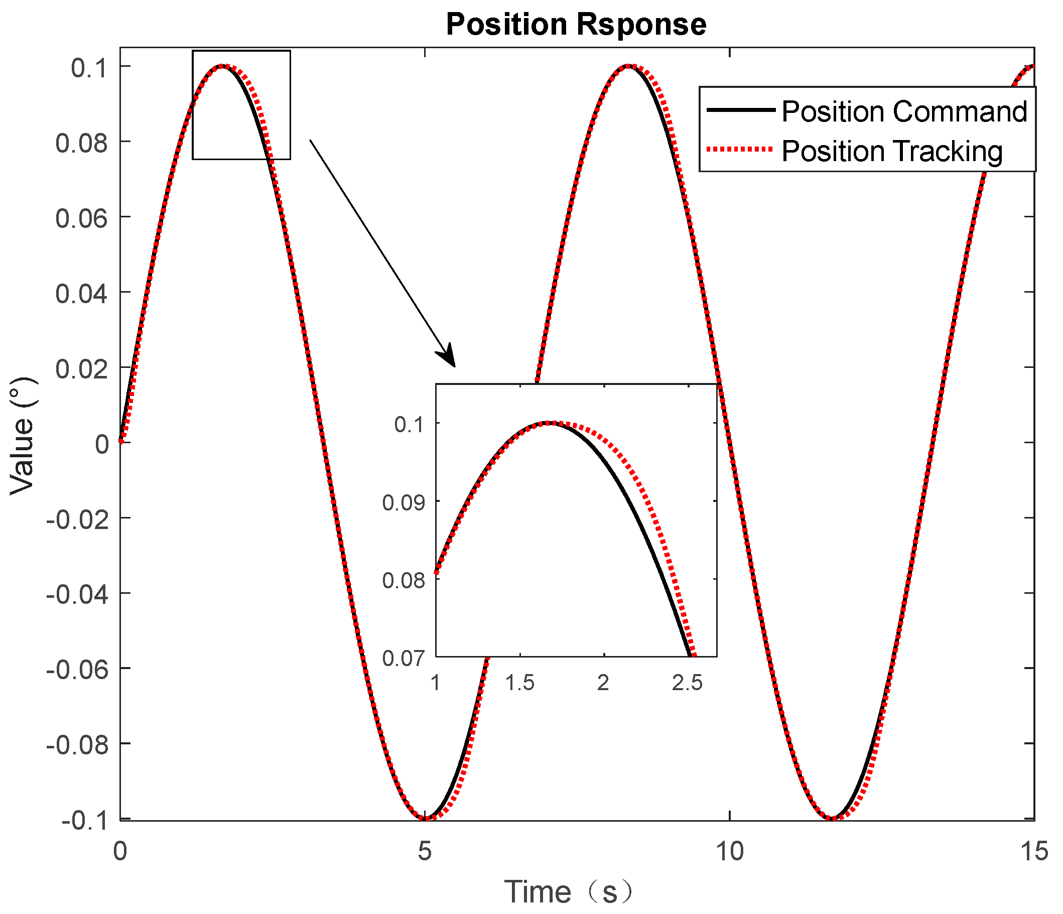
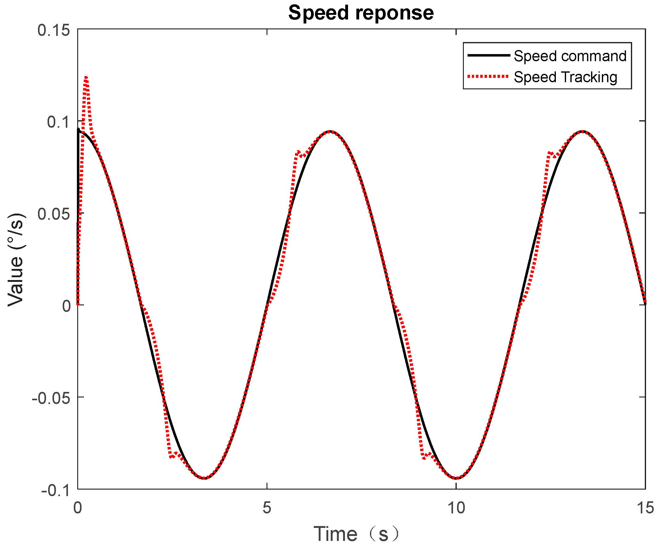
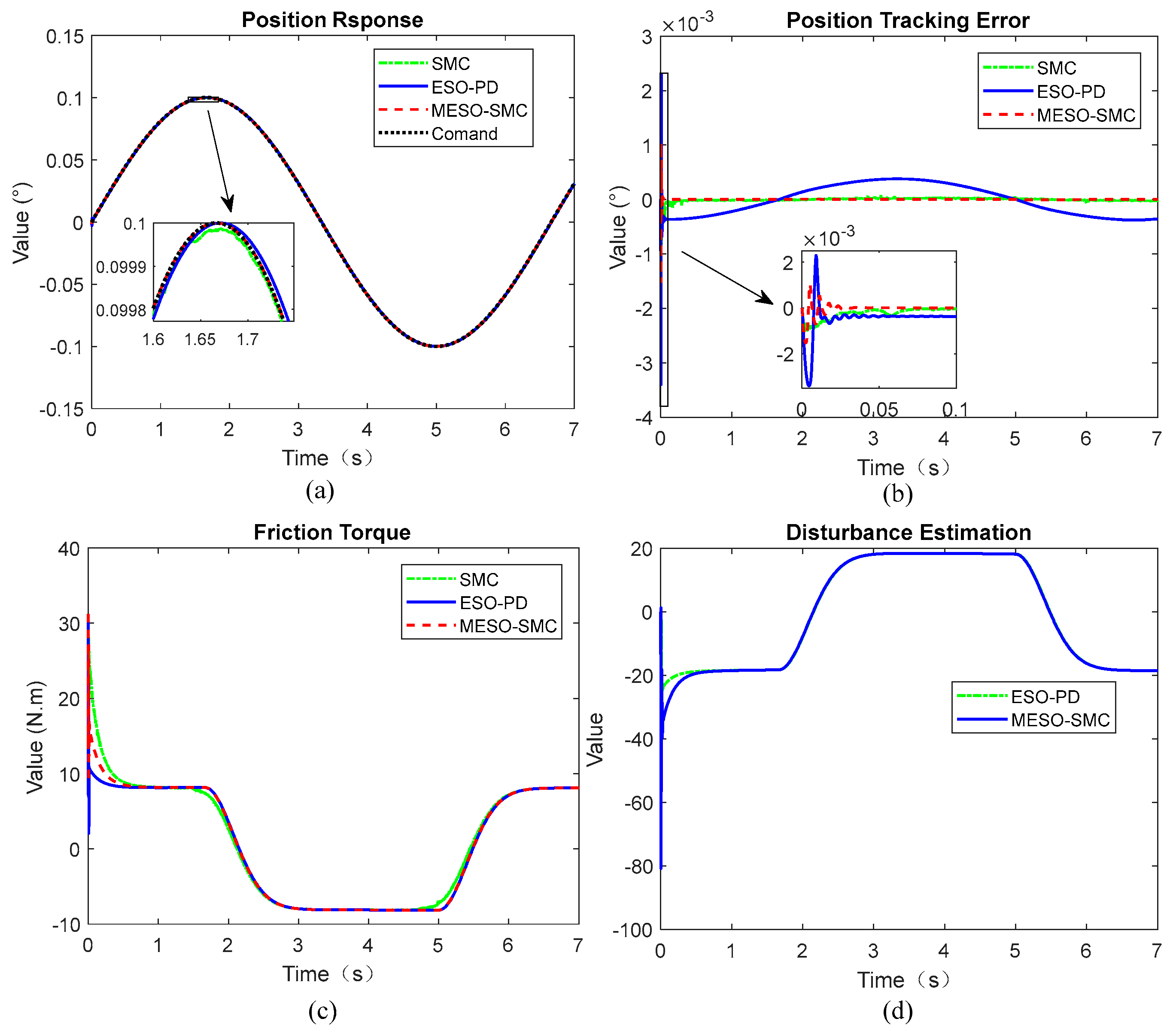
4.1. Low Frequency Tracking Performance

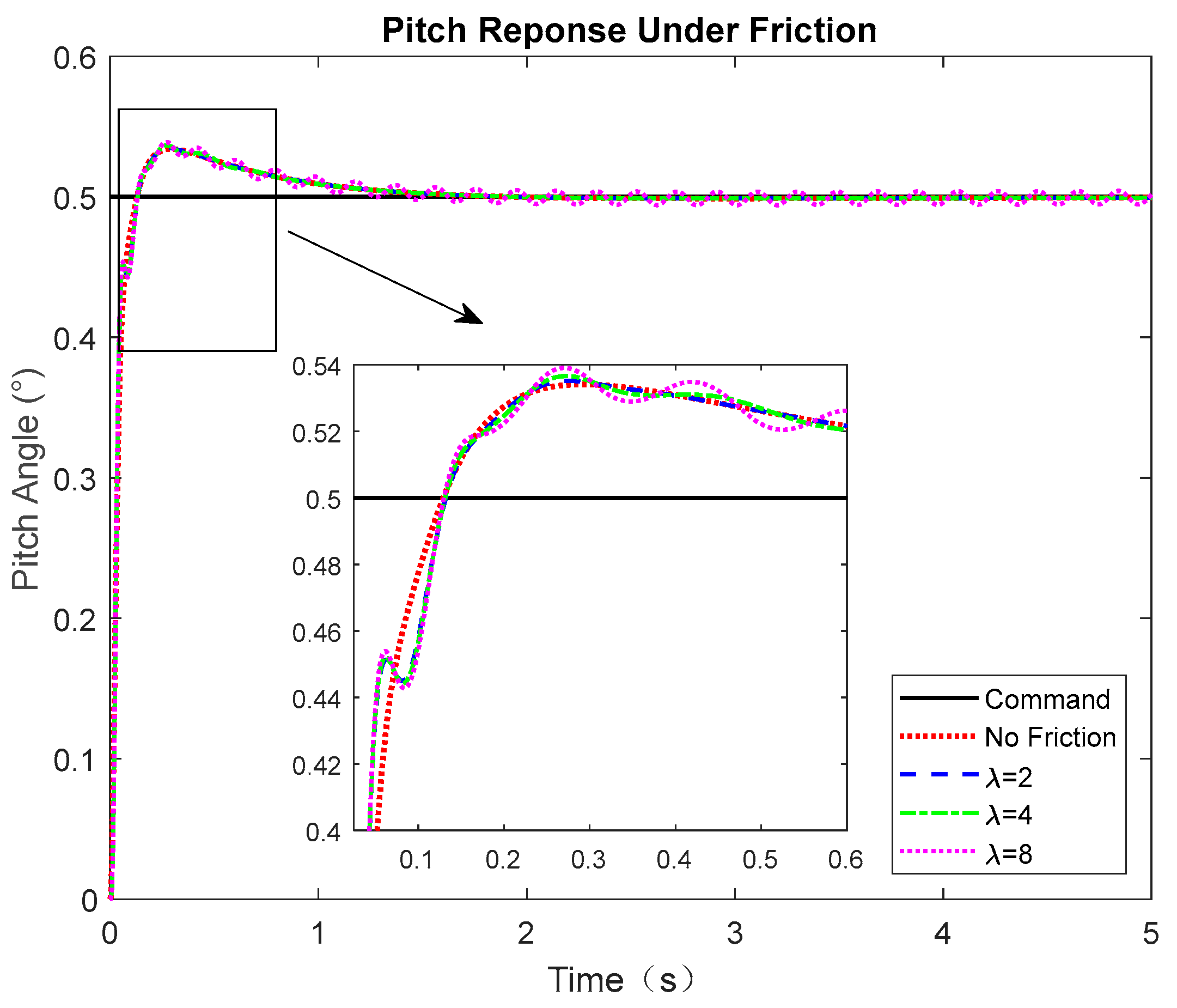
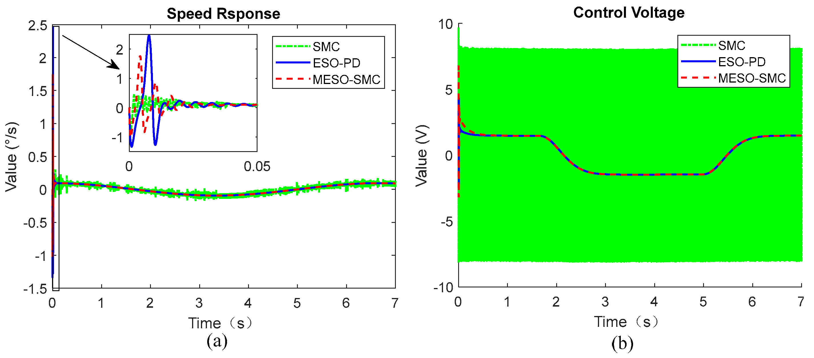
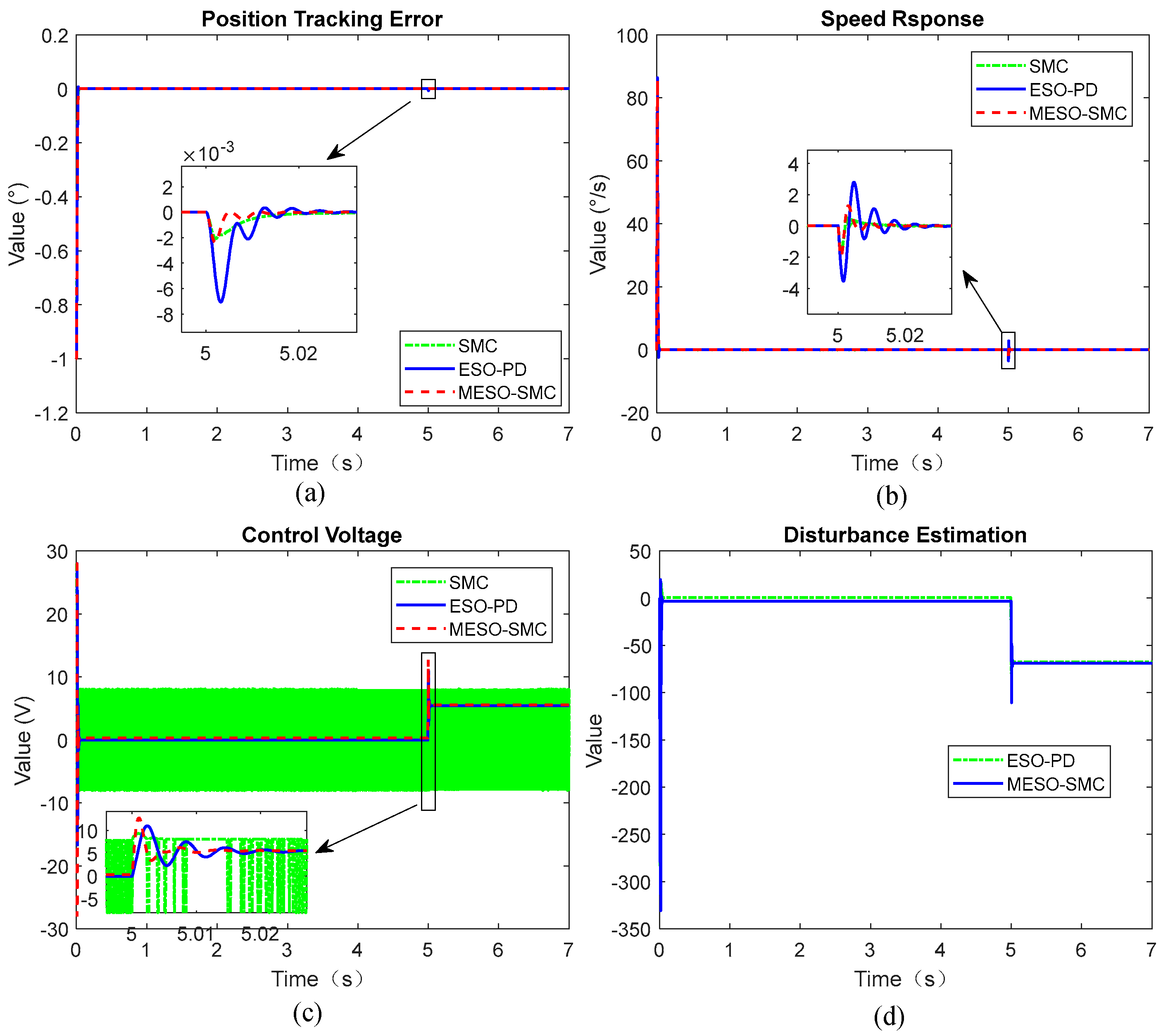
Simulation conditions: $\lambda =4$, no hinge torque, at a frequency of 0.15 Hz, amplitude of 0.1° sinusoidal command signal. Simulation results can be seen in Figure 11a,b.

It can be seen from Figure 11a that under the effect of friction nonlinearity, the speed curve under SMC has obvious chattering, while speed curves under ESO-PD and MESO-SMC are smooth. Figure 11b shows control voltage is chattering obviously under SMC, while the other two control methods have no chattering. Voltage chattering will cause speed chattering and undesirable vibration of mechanical equipment.

According to Figure 12a,b, under the action of friction nonlinearity, these three methods can track the position command, and the steady-state accuracy are all better than 5‰. It can be seen from Figure 12c that under different control, the friction torques are different due to the different velocity dynamics; under SMC control, the friction torques are slightly different from those under the other two control modes due to the speed chattering. Figure 12d shows the system disturbance can be estimated under both ESO and MESO. The estimated values of EMA are different in the initial stage but converge in the steady state.

4.2. Step Response

In the presence of friction nonlinearity and $\lambda =1$, the command signal is unit step, and the maximum hinge torque of 30 N. m is added from 5 s to the end, its dynamic response is shown in Figure 13.

Figure 13a shows that the three control methods have good tracking performance. The ESO-PD control has slight lag and overshoot when adding the hinge torque. Figure 13b shows that ESO-PD has the largest overshoot, the speed response performance under MESO-SMC is similar to that of SMC. Figure 13c shows SMC control voltage has a large chattering, and this phenomenon does not exist under the other two controllers. Figure 13d shows that the estimates of the two observers differ, but the trend is similar.

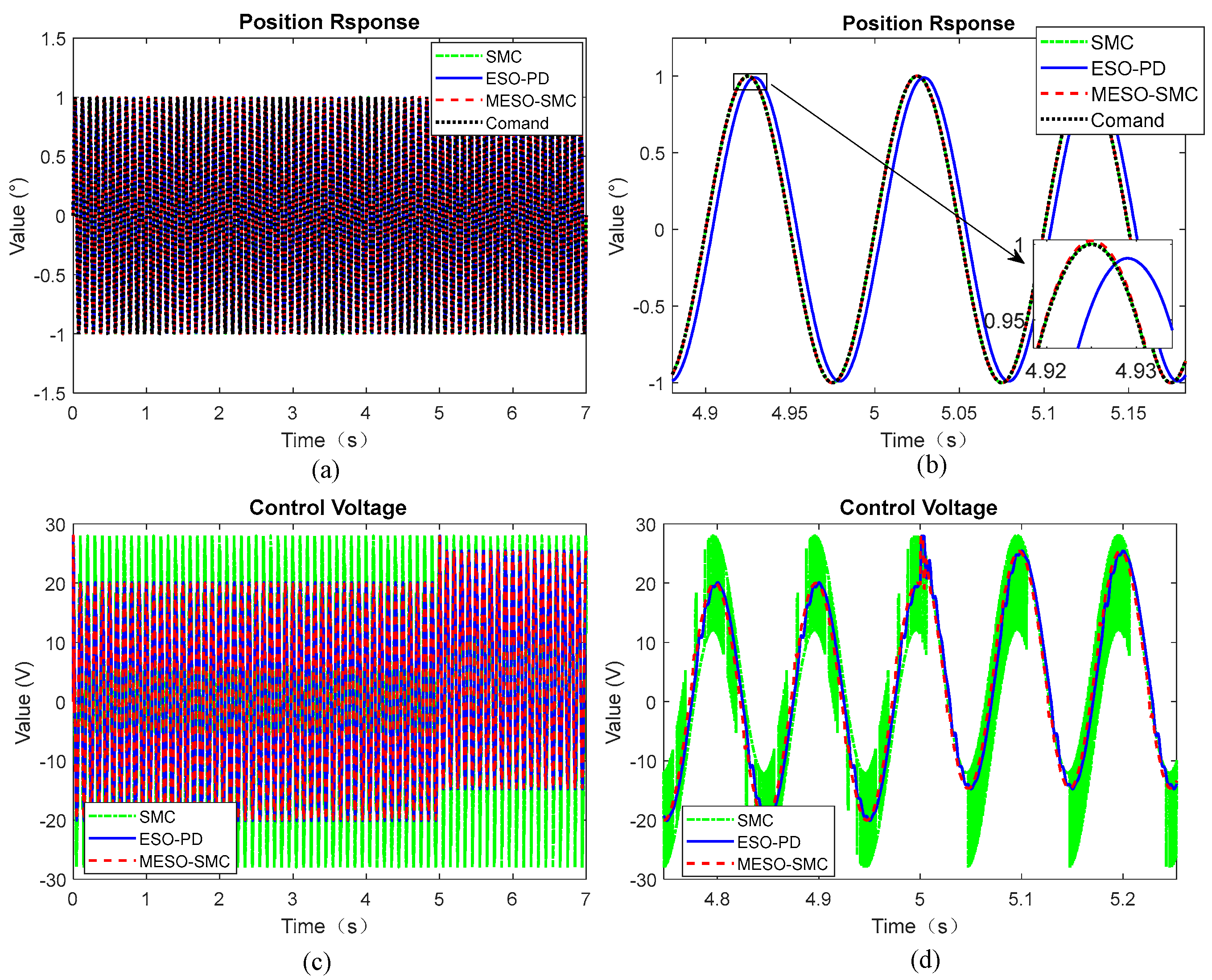
4.3. High-Frequency Dynamic Response

Considering the friction nonlinearity of EMA and $\lambda =1$, and the maximum hinge torque of 30 N. m is added from 5 s to the end, after 10 Hz sinusoidal signal commanding, its dynamic responses are shown in Figure 14, Figure 15 and Figure 16.

As shown in Figure 14a,b. Considering friction nonlinearity, hinge torque load has little influence on the control accuracy of the EMA system under simulation conditions, and both the MESO-SMC control method and SMC have strong robustness and tracking accuracy. But position tracking has a 14.4° phase lag and about 1% amplitude attenuation under ESO-PD control. According to Figure 14c,d, voltage chattering still exists under SMC, it is also observed that the control voltage can respond quickly without chattering under nonlinearity and hinge torque load, and dynamic performances are greatly improved by MESO-SMC.

As can be seen from Figure 15, due to phase lag of velocity, its friction torque also lags under ESO-PD control.

As shown in Figure 16a,b, under the simulation condition of 10 Hz, the proposed MESO can better estimate the system disturbance in real time. According to Figure 16c,d, it can be seen that there is certain tracking lag and distortion in the speed curve under the ESO-PD control method.

5. Conclusions

In this paper, to deal with the negative influence of the EMA friction nonlinearity of the flight vehicle on the flight attitude control, the friction compensation method of EMA is studied, the composite control strategy of SMC based on the MESO is proposed, and its theoretical analysis is given. By comparing the dynamic responses of the three different control strategies under different control commands, the superiority of the proposed control strategy is verified, and the following conclusions are drawn:

(1)

The MESO-SMC method in this paper has high position tracking accuracy, and the “flat top” and speed curve distortion phenomenon caused by friction are effectively compensated for.

(2)

In the case of high-frequency response, the position dynamics governed by the ESO-PD controller have a certain phase lag, and both MESO-SMC and SMC have good position tracking performance.

(3)

MESO-based controller has good estimation performance and can effectively estimate and compensate for internal and external disturbances.

(4)

Although SMC has good robustness, it will produce control chattering or even speed chattering. MESO-SMC can effectively suppress sliding mode chattering and achieve high-precision robust control.

In this paper, only the friction nonlinearity influence on the high-precision control of EMA is considered, and the modeling of EMA is simplified. However, there are still other nonlinearities such as backlash and dead zone in the actual EMA, these factors will be considered in further studies.

References

1. Wei, R.; Dong, Q.; Zhang, X.; Li, Z. Friction Compensation Control of Electromechanical Actuator Based on Neural Network Adaptive Sliding Mode. Sensors 2021, 21, 1508. [Google Scholar]
2. Merzouki, R.; Cadiou, J.C. Estimation of backlash phenomenon in the electromechanical actuator. Control Eng. Pract. 2005, 13, 973–983. [Google Scholar] [CrossRef]
3. Merzouki, R.; Davila, J.A.; Fridman, L.; Cadiou, J.C. Backlash phenomenon observation and identification in electromechanical system. Control Eng. Pract. 2007, 15, 447–457. [Google Scholar] [CrossRef]
4. Sun, G.; Zhao, J.; Chen, Q. Observer-based compensation control of servo systems with backlash. Asian J. Control 2019, 23, 499–512. [Google Scholar] [CrossRef]
5. Elmic, R.R.; Lewis, F.L. Deadzone compensation in motion control systems using neural networks. IEEE Trans. Autom. Control 2000, 45, 602–613. [Google Scholar] [CrossRef]
6. Zuo, Z.; Li, X.; Shi, Z. L1 adaptive control of uncertain gear transmission servo systems with deadzone nonlinearity. ISA Trans. 2015, 58, 67–75. [Google Scholar] [CrossRef]
7. Zuo, Z.; Ju, X.; Ding, Z. Control of Gear Transmission Servo Systems With Asymmetric Deadzone Nonlinearity. IEEE Trans. Control Syst. Technol. 2016, 24, 1472–1479. [Google Scholar] [CrossRef]
8. Fu, B.; Qi, H.; Xu, J.; Yang, Y.; Wang, S.; Gao, Q. Attitude Control in Ascent Phase of Missile Considering Actuator Non-Linearity and Wind Disturbance. Appl. Sci. 2019, 9, 5113. [Google Scholar] [CrossRef]
9. Deng, W.; Yao, J.; Ma, D. Robust adaptive precision motion control of hydraulic actuators with valve dead-zone compensation. Isa Trans. 2017, 70, 269–278. [Google Scholar] [CrossRef]
10. Man, Z.; Mao, D.; Zhang, M.; Guo, L.; Gong, M. A Hybrid Control with PID–Improved Sliding Mode for Flat-Top of Missile Electromechanical Actuator Systems. Sensors 2018, 18, 4449. [Google Scholar] [CrossRef]
11. Keck, A.; Zimmermann, J.; Sawodny, O. Friction parameter identification and compensation using the ElastoPlastic friction model. Mechatronics 2017, 47, 168–182. [Google Scholar] [CrossRef]
12. Khayati, K.; Bigras, P.; Dessaint, L.A. LuGre model-based friction compensation and positioning control for a pneumatic actuator using multi-objective output-feedback control via LMI optimization. Mechatronics 2009, 19, 535–547. [Google Scholar] [CrossRef]
13. Capace, A.; Merola, A.; Cosentino, C.; Amato, F. A Multistate Friction Model for the Compensation of the Asymmetric Hysteresis in the Mechanical Response of Pneumatic Artificial Muscles. Actuators 2019, 8, 49. [Google Scholar] [CrossRef]
14. Lrinc, M.; Béla, L. Identification and Model-based Compensation of Striebeck Friction. Acta Polytech. Hung. 2006, 3, 45–58. [Google Scholar]
15. Wang, S.; Wu, Q.; Yang, X. Active disturbance rejection control of friction for optoelectronic telescopes. Int. J. Simul. Syst. 2016, 17, 35.31–35.35. [Google Scholar] [CrossRef]
16. Freidovich, L.; Robertsson, A.; Shiriaev, A.; Johansson, R. LuGre-Model-Based Friction Compensation. IEEE Trans. Control Technol. 2009, 18, 194–200. [Google Scholar] [CrossRef]
17. Yu, H.; Gao, H.; Deng, H.; Yuan, S.; Zhang, L. Synchronization Control with Adaptive Friction Compensation of Treadmill-based Testing Apparatus for Wheeled Planetary Rover. IEEE Trans. Ind. Electron. 2021, 69, 592–603. [Google Scholar] [CrossRef]
18. Utkin, V.I.; Chang, H.C. Sliding mode control on electro-mechanical systems. Math. Probl. Eng. 2002, 8, 1–23. [Google Scholar] [CrossRef]
19. Fallaha, C.J.; Saad, M.; Kanaan, H.Y.; Al-Haddad, K. Sliding-Mode Robot Control With Exponential Reaching Law. IEEE Trans. Ind. Electron. 2011, 58, 600–610. [Google Scholar] [CrossRef]
20. Shepit, B.M.; Pieper, J.K. Sliding mode control design for complex valued sliding manifold. In Proceedings of the 40th IEEE Conference on Decision and Control (Cat. No.01CH37228), Orlando, FL, USA, 4–7 December 2001. [Google Scholar]
21. Difonzo, F.V. A note on attractivity for the intersection of two discontinuity manifolds. Opusc. Math. 2020, 40, 685–702. [Google Scholar] [CrossRef]
22. Haddad, W.M.; Chellaboina, V. Nonlinear dynamical systems and control. In Nonlinear Dynamical Systems and Control; Princeton University Press: Princeton, NJ, USA, 2011. [Google Scholar]
23. Liu, J.; Sun, F. Research progress of sliding mode variable structure control theory and algorithm. Control Theory Appl. 2007, 24, 407–418. [Google Scholar] [CrossRef]
24. Wang, S.; Chen, Q.; Ren, X.; Yu, H. Neural network-based adaptive funnel sliding mode control for servo mechanisms with friction compensation. Neurocomputing 2020, 377, 16–26. [Google Scholar] [CrossRef]
25. Deng, W.; Yao, J. Extended-State-Observer-Based Adaptive Control of Electro-Hydraulic Servomechanisms without Velocity Measurement. IEEE ASME Trans. Mechatron. 2019, 25, 1151–1161. [Google Scholar] [CrossRef]
26. Deng, W.; Yao, J.; Yaoyao, W.; Xiaowei, Y.; Jiuhui, C. Output feedback backstepping control of hydraulic actuators with valve dynamics compensation. Mech. Syst. Signal Processing 2021, 158, 107769. [Google Scholar] [CrossRef]
27. Deng, W.; Yao, J.; Ma, D. Time-varying input delay compensation for nonlinear systems with additive disturbance: An output feedback approach. Int. J. Robust Nonlinear Control 2018, 28, 31–52. [Google Scholar] [CrossRef]
28. Ren, C.; Li, X.; Yang, X.; Ma, S. Extended State Observer based Sliding Mode Control of an Omnidirectional Mobile Robot with Friction Compensation. IEEE Trans. Ind. Electron. 2019, 66, 9480–9489. [Google Scholar] [CrossRef]
29. Shin, W.H.; Lee, S.J.; Lee, I.; Bae, J.S. Effects of actuator nonlinearity on aeroelastic characteristics of a control fin. J. Fluids Struct. 2007, 23, 1093–1105. [Google Scholar] [CrossRef]
30. Canudas, d.W.C.; Olsson, H.; Astrom, K.J.; Lischinsky, P. A new model for control of systems with friction. IEEE Trans. Autom. Control 1995, 40, 419–425. [Google Scholar] [CrossRef]
31. De Wit, C.C.; Lischinsky, P. Adaptive friction compensation with partially known dynamic friction model. Int. Comm. Radiat. Units Meas. 1997, 11, 65–80. [Google Scholar] [CrossRef]
32. Wei, Y.U.; Jia-Guang, M.A.; Jin-Ying, L.I.; Xiao, J. Friction parameter identification and friction compensation for precision servo turning table. Opt. Precis. Eng. 2011, 19, 2736–2743. [Google Scholar] [CrossRef]
33. Awouda, A.; Mamat, R.B. New PID Tuning Rule Using ITAE Criteria. In Proceedings of the 2010 the 2nd International Conference on Computer and Automation Engineering (ICCAE), Singapore, 26–28 February 2010; pp. 171–176. [Google Scholar]
34. Utkin, V.I. Sliding mode control design principles and applications to electric drives. IEEE Trans. Ind. Electron. 2002, 40, 23–36. [Google Scholar] [CrossRef]
35. Gao, W.; Wang, Y.; Homaifa. Discrete-time variable structure control systems. IEEE Trans. Ind. Electron. 1995, 42, 117–122. [Google Scholar]
36. Olsson, H.; Strm, K.J.; Wit, C.; Gfvert, M.; Lischinsky, P. Friction Models and Friction Compensation. Eur. J. Control 1998, 4, 5517–5522. [Google Scholar] [CrossRef] [Green Version]
37. Han, J. The Technique for Estimating and Compensating the Uncertainties: Active Disturbance Rejection Control Technique, 4th ed.; National Defense Industry Press: Beijing, China, 2008. [Google Scholar]
38. Guo, B.Z.; Zhao, Z.L. On the convergence of an extended state observer for nonlinear systems with uncertainty. Syst. Control Lett. 2011, 60, 420–430. [Google Scholar] [CrossRef]
39. Petros, A.; Ioannou, J.S. Robust Adaptive Control; Prentice Hall: Hoboken, NJ, USA, 1995. [Google Scholar]
Figure 1. Schematic diagram of EMA system.
Actuators 11 00265 g001
Figure 2. Diagram of simplified EMA model with friction.
Actuators 11 00265 g002
Figure 3. Position response under friction.
Actuators 11 00265 g003
Figure 4. Speed response under friction.
Actuators 11 00265 g004
Figure 5. Block diagram of longitudinal attitude control.
Actuators 11 00265 g005
Figure 6. Bode diagrams of the model at the feature point: (a) Open loop bode diagram. (b) Close loop bode diagram under PID control.
Actuators 11 00265 g006
Figure 7. Pitch response under friction.
Actuators 11 00265 g007
Figure 8. Composite SMC control diagram of EMA.
Actuators 11 00265 g008
Figure 9. Error feedback function gain curves comparison.
Actuators 11 00265 g009
Figure 10. Curve of f ( e 1 ) .
Actuators 11 00265 g010
Figure 11. Speed and control voltage comparisons. (a) Speed response. (b) Control voltage.
Actuators 11 00265 g011
Figure 12. Comparisons of low-frequency simulation: (a) Position tracking. (b) Position tracking errors. (c) Friction torque curves. (d) Disturbance estimation.
Actuators 11 00265 g012
Figure 13. Step response comparations. (a) Position tracking. (b) Speed response. (c) Control voltage. (d) Disturbance estimation.
Actuators 11 00265 g013
Figure 14. High-frequency dynamic simulation comparisons. (a) Position tracking. (b) Local curves of (a). (c) Control voltage. (d) Local curves of (c).
Actuators 11 00265 g014
Figure 15. Friction torque curves.
Actuators 11 00265 g015
Figure 16. Disturbance estimation and velocity response. (a) Disturbance estimation curves. (b) Local curves of (a). (c) Velocity response curves. (d) Local curves of (c).
Actuators 11 00265 g016