Abstract
In this study, an adaptive dynamic programming (ADP) control strategy based on the strain measurement of a fiber Bragg grating (FGB) sensor array is proposed for the vibration suppression of a complicated flexible-sloshing coupled system, which usually exists in aerospace engineering, such as launch vehicles with a large amount of liquid propellant as well as a flexible beam structure. To simplify the flexible-sloshing coupled dynamics model, the equivalent spring-mass-damper (SMD) model of liquid sloshing is employed, and a finite-element method (FEM) dynamic model for the beam structure coupled with the liquid sloshing is mathematically established. Then, a strain-based vibration dynamic model is derived by employing a transformation matrix based on the relationship between displacement and strain of the beam structure. To facilitate the design of a strain-based control, a tracking differentiator is designed to provide the strains’ derivative signals as partial states’ estimations. Feeding the system with the strain measurements and their derivatives’ estimations, an ADP controller with an action-dependent heuristic dynamic programming structure is proposed to suppress the vibration of the flexible-sloshing coupled system, and the corresponding Lyapunov stability of the closed-loop system is theoretically guaranteed. Numerical results show the proposed method can effectively suppress coupled vibration depending on limited strain measurements irrespective of external disturbances.
1. Introduction
Flexible-sloshing coupling problems are crucial in many fields [1], such as aerospace, architecture, and ocean engineering. Particularly in aerospace fields [2], modern spacecraft typically carry a large amount of liquid fuel and are also equipped with large flexible structures such as solar panels, communication antennae, and space manipulators. During attitude and orbit motion, the spacecraft is easily disturbed by liquid sloshing and flexible appendage vibrations. For flexible-sloshing coupling systems, elastic vibration can trigger liquid sloshing, resulting in the production of sloshing forces. Additionally, the coupling of sloshing and elastic vibration exerts a profound influence on the performance of the systems [3]. Therefore, the coupling dynamic and control of elastic vibration and liquid sloshing have received significant attention. In response to this issue, researchers continue to study the influence of structural elasticity and liquid sloshing on the control system. Specifically, they have (1) established equivalent beam models for elastic vibration [4]; (2) established equivalent mechanical models for liquid sloshing, including the spring-mass-damper model [5,6], single pendulum model [7], etc.; (3) modified equivalent models through ground modal analysis [8] and experimentation [9].
For elastic vibration, specific devices such as displacement sensors and accelerators can be employed to obtain vibration motion parameters, while the accelerators and gyroscopes installed on structures primarily serve to provide motion parameters for control systems. In these systems, error signals resulting from vibration-induced deformations can influence the accuracy of control performance. In contrast, fiber Bragg grating (FBG) sensors exhibit advantages, including lighter weight, stronger resistance to electromagnetic interference, easier integration, and higher accuracy. Therefore, they can be more conveniently integrated with control systems [10,11,12]. In addition, the exploration of sloshing dynamics encompasses theoretical analysis, numerical simulation, experimental methods, and theoretical and numerical synthesis methods. In the 1960s, NASA provided an analytical solution for the sloshing dynamics of several fixed-shape tanks [13]. Meanwhile, the advancement of computational fluid dynamics (CFD) technology has enabled more precise modeling of sloshing dynamics through FEM, the boundary element method, and finite difference method. Nevertheless, due to the constraints of onboard computer speed, memory, and the intricate nature of sloshing dynamics, a simple and efficient method is still required to replace complex calculation tasks in practical applications. Therefore, equivalent mechanical models are commonly employed in engineering to depict liquid sloshing by capturing sloshing patterns inside the tank using the motion of a rigid body [13].
In engineering practice, some novel vibration control devices, such as the tuned mass damper (TMD) [14] and negative stiffness mechanisms [15] (KDamper [16,17]), have been widely used. In addition, in the field of control algorithms, the classical control theory has been applied with great maturity. However, the classical controller can no longer satisfy the demand for stability in flexible-sloshing coupling systems. In response to practical needs [18,19] and theoretical challenges [20], several control methods have received great attention, including positive position feedback (PPF) control [21,22], independent modal space control (IMSC) [23,24], sliding mode control [25], boundary control [26,27], adaptive control [28], and intelligent control [29,30,31,32]. Among them, the PPF method is used to select the appropriate zeros and poles of the second-order filter to ensure the stability margin of closed-loop systems. The PPF method was first proposed in [21], and a modified PPF vibration active control method based on an adaptive controller was proposed in [22]. Vibration active control based on PPF can be numerically simulated to prove the effectiveness of this algorithm. The IMSC method involves discretizing the control object into various modal features of different orders and controlling the discrete modes. Active vibration control methods based on IMSC, as proposed in [23,24], can effectively suppress vibration. In [25], a sliding mode controller that only uses boundary information is proposed for the stabilization problem of an Euler–Bernoulli beam system. Boundary control is recognized as a highly practical approach for vibration control of flexible structures. In [26], a novel barrier Lyapunov function was employed to design a vibration boundary controller for an Euler–Bernoulli beam with boundary output constraints. This approach successfully suppressed beam vibrations without violating the constraints. Additionally, for the problem of vibration attenuation of Euler–Bernoulli beam systems with imprecise system parameters, external disturbances, asymmetric input saturation, and output constraint, the boundary controllers in [27,28] were designed by constructing adaptive laws. Furthermore, intelligent control has received significant attention due to its robust self-learning and self-adaptive ability. Ref. [29] conducted a study on the delay feedback control of cantilever vibration based on a genetic algorithm. Ref. [30] proposed a decomposed parallel fuzzy control with the adaptive neuro-fuzzy concept. Additionally, [31,32] proposed active vibration control algorithms based on reinforcement learning (RL). In particular, the adaptive dynamic programming (ADP) method, which leverages a critic-action network structure based on RL, has gained widespread recognition [33]. This approach boasts two key advantages: (1) ADP operates as a data-driven learning control method, eliminating the need for mathematical models; (2) the parameters of ADP can be adaptively updated over time when the system is disturbed. Drawing from these advantages, the ADP method is considered in this paper for vibration and sloshing suppression control.
In summary, this paper explores the control of a beam attached to a tank. To construct the flexible-sloshing coupling dynamic model, the vibration of the beam is analyzed using an Euler–Bernoulli beam and FEM, while the liquid sloshing in the tank is equivalent to a spring-mass-damper model. Drawing on the benefits of FBG sensors, a vibration and sloshing suppression control algorithm based on FBG strain information is developed in this paper. A strain-based vibration dynamic model is established by employing a transformation matrix that relies on the relationship between displacement and strain. Additionally, a tracking differentiator is designed to provide real-time first-order derivatives of the strain. Finally, based on the strain-based vibration dynamic model, an ADP method based on FBG strain information is proposed to suppress elastic vibration and sloshing. The main innovations of this paper are as follows:
- (1)
- Compared with complex dynamic models, the Euler–Bernoulli beam model and spring-mass-damper equivalent model provide a simpler and more convenient way to construct the flexible-sloshing coupling dynamic model. The development of a strain-based vibration dynamic model facilitates the full utilization of FBG sensors’ information.
- (2)
- Compared with control methods that require motion parameters, the control method proposed in this paper can effectively suppress elastic vibration and sloshing even when only partial strain information is applied. Furthermore, the utilization of FBG strain information allows for direct measurement, eliminating the need for estimation of vibration parameters. This controller’s advantages in practicality make it highly suitable for engineering applications.
The rest of the paper is organized as follows. In Section 2, the flexible-sloshing coupling dynamic model and the strain-based vibration dynamic equation are described. Section 3 presents the ADP controller based on FBG strain information and corresponding theoretical analysis. Numerical simulations are provided in Section 4. Finally, Section 5 concludes this paper.
2. Preliminaries and System Descriptions
2.1. Flexible-Sloshing Coupling Dynamic Model
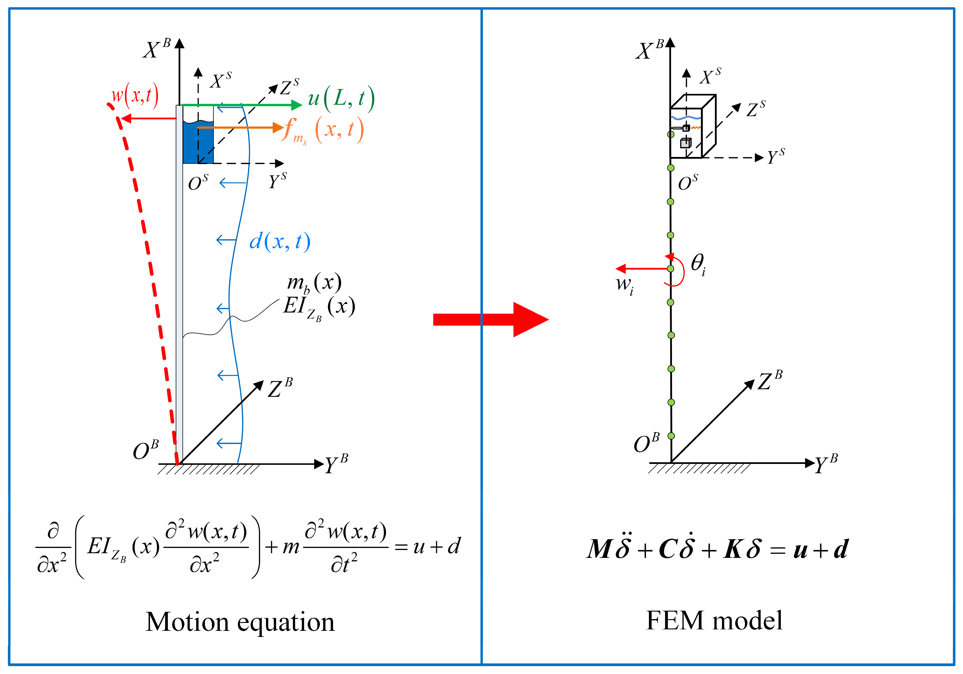
As illustrated in Figure 1, to investigate the flexible-sloshing coupling dynamic model, a combined structure consisting of a tank attached to a beam is considered. The vibration of the beam stimulates the liquid sloshing within the tank, which in turn generates a sloshing force that impacts the tank and alters the vibration of the beam.
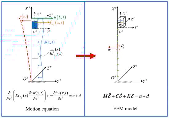
Figure 1.
Flexible-sloshing coupling system including spring-mass-damper model and Euler–Bernoulli cantilever beam’s FEM model.
Assumption 1.
The flexible-sloshing coupling dynamic model is applicable to the case of small amplitude vibration and sloshing. The beam is slender and uniform, i.e., the shear deformation is not considered [34]. In addition, the spring-mass-damper model must satisfy the conditions that the liquid in the tank is incompressible, non-viscous, and non-rotating [35].
According to Figure 1, the base coordinate system and the tank coordinate system are established. The origins and are located at the end of the beam and the center of the tank’s bottom, respectively. Both coordinate systems are right-hand systems. Note that the base coordinate system is a global coordinate system, and the tank coordinate system changes with the vibration of the beam. is the rotation transformation matrix from the tank coordinate system to the base coordinate system, which is defined as
where is the rotation angle of the beam’s position relative to the origin of the tank coordinate system in the base coordinate system, which varies with time.
Further, is the mass of the beam; is the bending stiffness with respect to axis; is the transverse displacement of the beam related to time and the position on the beam ; is the length of the beam; is control input acts on the end of the structure; represents the unknown disturbance force applied to the beam; denotes the sloshing force in the tank coordinate system. Note that and are distributed load and concentrated load, respectively.
Assumption 2.
For the unknown disturbance , we assume that there exists a constant , such that , . The time-varying has finite energy and, thus, is bound, i.e., [26].
Remark 1
[36]. When the force acting on the beam is distributed load, the unit force of is provided as
and the unit force of concentrated load is
where is the Hermite shape function, and is the coordinate of position where acts on the beam. We define , and is provided as
The analytical solution of the Euler–Bernoulli cantilever beam’s motion equation is difficult to obtain in the case of non-uniform inertia and stiffness properties. So the FEM is often used to model the motion of the beam, and the second-order differential Equation [4] is obtained:
which includes beam nodes and can be considered as a degree-of-freedom system. Each node consists of two degrees of freedom, namely translation and rotational , i.e.,
, , and are the mass, damping, and stiffness matrices, respectively. and are assembled by the following elemental matrices:
where is the length of the beam’s element. Additionally, the corresponding damping matrix is .
By introducing the influence of the sloshing force , Equation (2) becomes
where , , and are mass, damping, and stiffness matrices, and represents the force driving the coupling system, including control force , disturbance , and sloshing force .
As shown in Figure 2, the spring-mass-damper equivalent mechanical model is employed in this paper to estimate the liquid sloshing force. The liquid sloshing dynamic model in the tank can be regarded as a spring-mass-damper system [6], allowing for the calculation of the sloshing force . The mass of the liquid in the tank is , and the spring-mass-damper system divides the liquid into sloshing mass and non-sloshing mass . On the translation plane, along the two axes perpendicular to the central axis of the tank, the sloshing mass is connected to the tank through springs and dampers. Therefore, the sloshing mass is a secondary damping vibration perpendicular to the symmetry axis.
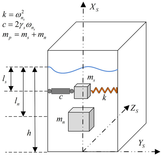
Figure 2.
Spring-mass-damper model.
The mass of the liquid is
where is the density of the liquid, is the length of the bottom side of the tank, and is the height of the liquid level.
According to Equation (6), can be calculated as
For the first-order sloshing mode of the rectangular tank, according to Section 5.2 of [37], the following equivalent parameters are established.
where and are the distances of sloshing and non-sloshing mass from the free liquid surface, respectively. is elastic constant, and the relation between it and natural frequency is .
Note that the energy dissipation model in the oscillating system is approximately provided by the equivalent second-order damping ratio . Due to the lack of effective data for the tank design, according to [38], the equivalent second-order damping ratio of all sloshing modes is presumed to be .
According to [35], the dynamic equation of liquid sloshing is as follows:
where represents the perturbation from the nominal reference. only selects the axial acceleration component and only selects the normal component. The sloshing mass acceleration relative to the body in the axial direction is zero. is
and the rotation term is
The force generated by the sloshing liquid is opposite to the force exerted on the liquid by the translation and rotation of the body, and the axial acceleration of the sloshing mass relative to the body must be considered. Assuming that most of the acceleration occurs along the axis, this component acts on the force applied by the sloshing mass such that:
Note that acts on the beam as a concentrated load.
2.2. Strain-Based Vibration Dynamic Model
In this paper, the strain information is used to design the controller for the system (5). To acquire the strain-based vibration dynamic model, the relationship [39] between the strain and the node displacement of the beam is established as
The element transfer matrix [40] is
where is the height of the beam’s cross-section.
Thus, Equation (13) is written as
According to Equation (15), Equation (5) is rewritten as
The dynamic model can be obtained as
where , , and are the mass, damper, and stiffness matrices, which satisfy , , and . Additionally, force is provided as
By defining variables , the state equation with strain and the first-order derivatives of the strain as state variables can be obtained as follows:
In engineering applications, due to the installation of FBG sensors at regular intervals on the structure, only the strain values at some locations on the structure can be measured. Therefore, Equation (18) is rewritten as
where is the reduced state vector, and and are the system matrices.
The dimension of the dynamic model (18) is , and represents the number of elements divided by FEM. To ensure accuracy, the value of is relatively high, which will make real-time calculations on the onboard computer challenging. Therefore, the dimension of the system (19) is set as , and is the number of FBG sensors, such that the dimension of the system is reduced.
Remark 2.
The above method of associating the dimension of the system with the actual number of FBG sensors can better meet the requirements of engineering. This method has the same effect as the dynamic model reduction technology, which includes two main types: the physical reduce-order model and the agent model. The agent model is used to approximate the original complex structure through mathematical expressions with less computation, and the characteristics of the complex structure are obtained in the form of solving mathematical expressions, including the artificial neural network model. On the other hand, a neural network-based ADP control method is adopted in this paper. As a type of agent model, a neural network takes partial strain information as the input, which can better reflect the response characteristics of the whole structure. Moreover, the proposed ADP method in this paper is an optimal control method, which enables the elastic vibration and sloshing suppression control of the beam on the basis of only partial strain information through reasonable parameters design of the ADP method.
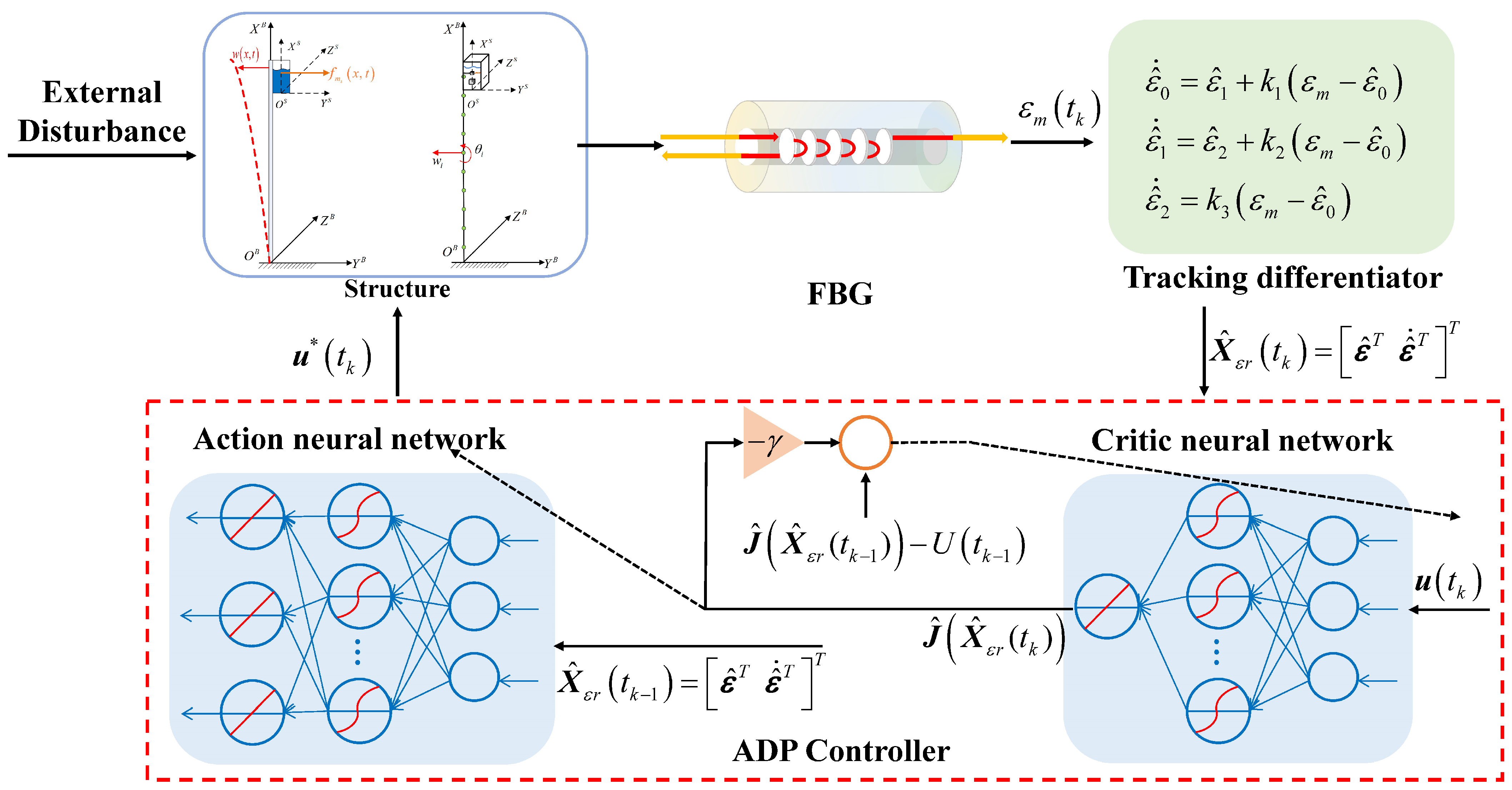
On the other hand, FBG can only measure the strain value and cannot directly measure the first-order derivative of the strain . Hence, it is necessary to introduce a tracking differentiator to estimate the state vector . According to references [12,41], the tracking differentiator is designed as follows:
where are the designed parameters; is the strain value measured by FBG; is the states of the differentiator. The real-time designed differentiator provides estimations of strain and its first-order derivative from the measurement .
Note that, according to [12], the estimation errors of the tracking differentiator (20) exponentially converge into a region of hyperball when given an appropriate choice of . This paper does not describe the proof process, and the detailed process is shown in [12]. In summary, based on the characteristics of the proposed differentiator, the states and are used as the estimations of the strain measurement as well as its first-order derivative .
Substituting the estimations of tracking differentiator into Equation (19), we can obtain
where . According to the strain-based vibration dynamic model (21), the intelligent controller is designed in the next section.
3. Control Strategy Design
3.1. Design of ADP Control Method Based on Strain Information of FBG
This paper proposed an ADP control method based on FBG strain information and neural networks. In contrast to previous work using motion parameters or modal parameters, this method can enable control performance using only strain information. The basic strategy of ADP [42] entails utilizing function approximators, such as linear function and neural network approximators, to construct critic networks to approximate the performance index function in the Hamilton–Jacobi–Bellman (HJB) function. For Equation (21), action-dependent heuristic dynamic programming (ADHDP) is adopted, and the system diagram is shown in Figure 3.
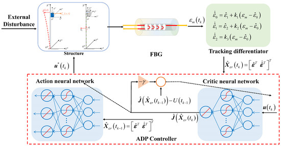
Figure 3.
Vibration control for flexible-sloshing system based on FBG information and ADHDP.
First, the cost function with a discount factor is defined as follows:
where is produced for the infinite horizon problem. is the utility function, and the quadratic performance index [33] is the most commonly used; that is,
where and are state and input utility weight matrices and positive-definite diagonal matrices.
The goal of the proposed method is to determine the appropriate control input to minimize . We define as the optimal cost function, which is shown as
Based on the optimal control theory, satisfies the following Bellman equation:
ADHDP adopts an action-critic network structure to obtain the approximate solution of the Bellman equation. The input of the critic network is the state and control input of the system, and the output is the estimation of . The action network’s input and output are, respectively, the state of the system and the approximate optimate control input . In addition, both the action and critic networks adopt the three-layer neural network, which contains the input, hidden, and output layers. A hyperbolic tangent transfer function [33] is used as the activation function . For any variable , the hyperbolic tangent transfer function is defined as follows:
Remark 3
[43]. The approximation error of the neural network can be arbitrarily small as long as there are enough hidden layer neurons when the weights of the input layer–hidden layer are randomly initialized and kept constant. Consequently, in the learning process of the critic and action neural network, this paper only updates the weights of the hidden output layer. The update rules adopt the gradient descent method, which will be described later.
The design of the critic neural networks is
where and are the weight matrices of the hidden input and hidden output layers.
To train the critic network through the backpropagation method, the prediction error is defined as follows:
Then, the error function to be minimized by the critic network is
The output of the action network, namely the optimal control strategy, is
where and are the weight matrices of the hidden input and hidden output layers.
The prediction error is defined as the difference between the estimated cost function and the desired ultimate object function , which is backpropagated to the network to train the action network. The expression of is
The error function to be minimized by the action network is
The purpose of the controller proposed in this paper is to make the whole structure stable; that is, the FBG strain value is zero as a result. Hence, we can set the desired ultimate object function to .
Note that, according to Remark 3, and are randomly initialized and kept constant, and and are updated based on the gradient descent method. Therefore, the expression of weight updating policy by the chain rule is
where and denote the learning rates of the critic and action networks, respectively.
3.2. Stability Analysis
This section will analyze the Lyapunov stability of the above control system. Firstly, the following assumptions and lemmas are held.
Assumption 3.
Let and are the optimal weights of the hidden output layer in the critic and action neural network. Both of them are bound, i.e., , , where and are positive, satisfying the following equations:
Lemma 1
[44]. Assumption 3 is held. The outputs of the critic and action networks are (26) and (29). The weights and of the critic and action networks are initialized and remain unchanged after initialization. The weights and are updated based on (32) and (33). Then, the errors between the optimal weights, and , and the weights and , obtained based on the above update rules, are uniformly ultimately bound.
The proof process of Lemma 1 can be seen in [44] and is not repeated in this paper. According to Lemma 1, when the neural network settings and weight updating rules are used in this paper, the estimation errors of the critic and action networks are uniformly ultimately bound [44]; that is, the method proposed in this paper can obtain the optimal control law.
Theorem 1.
For the dynamic model (21), the control law (29) is designed. If Assumption 3 and Lemma 1 are satisfied, the flexible-sloshing coupling control system is uniformly ultimately bounded.
Proof of Theorem 1.
Consider the Lyapunov function candidate defined as follows:
The time derivative of (34) is
Substituting (21) into (35) yields
According to the control law (29), (36) is rewritten as
where satisfies
In this paper, the flexible-sloshing coupling system is simplified according to the actual physical system, and the parameters in the actual physical system are bound, so the parameters of the proposed systems are bound; that is, , , , , and and are bound. The weight is bound according to Assumption 3 and Lemma 1. Based on the definition of the hyperbolic tangent transfer function, , then is bound; is a positive-definite diagonal matrix and is bound. In summary, we can see that is bound. Therefore, the system (21) based on the proposed control law (29) is uniformly ultimately bound [45].□
4. Numerical Simulations
The following numerical simulation demonstrates the effectiveness of the proposed ADP control strategy with strain information compared with the PD controller. An aluminum alloy cantilever beam and a cuboid tank are considered in this simulation. This tank is lightweight and thin-walled, so its weight can be ignored. The liquid in the tank is water. The parameters of the combined structure are shown in Table 1.

Table 1.
Parameters of the structure.
The initial conditions in this simulation are provided as , , and . The parameters of the tracking differentiator are set as , , and , where satisfies . The damping matrix is set as . The simulation time is 0.001s, and the total simulation time is 15s. A sinusoidal disturbance is applied. The dynamic responses of the structure are examined in the following cases.
Free Case: There is no control input in this simulation, i.e., , and the spatial time representation is shown in Figure 4.
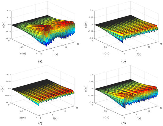
Figure 4.
Displacement of the structure in (a) free case; (b) ADP case 1 with 10 sensors; (c) ADP case 2 with 20 sensors; (d) PD case.
ADP Case 1: The ADP controller applies 10 FBG sensors’ information. The number of hidden layer nodes is 30, the learning rates are , and the state and input utility weight matrices are and . The spatial time representation is shown in Figure 5.
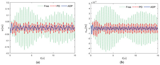
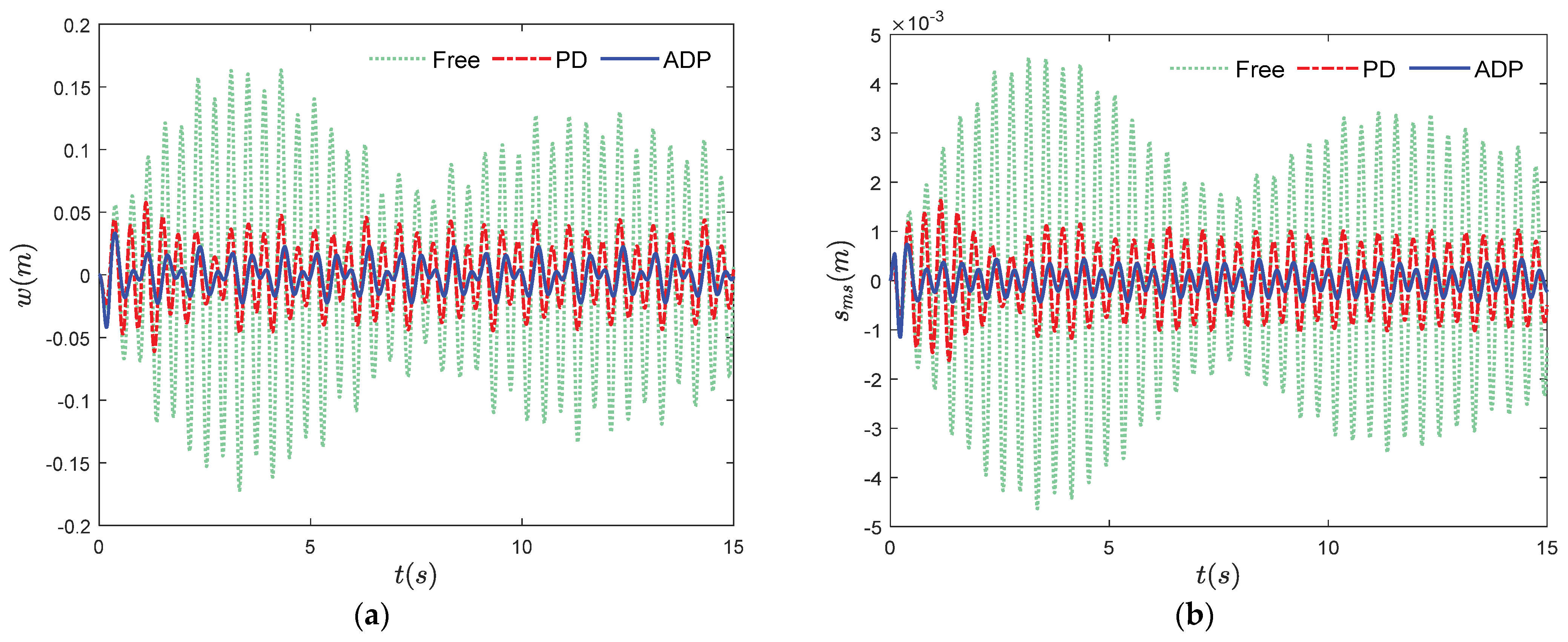
Figure 5.
Results of displacement. (a) Displacement of the structure’s free end in free case, PD case, and ADP case 1; (b) sloshing displacement in free case, PD case, and ADP case 1.
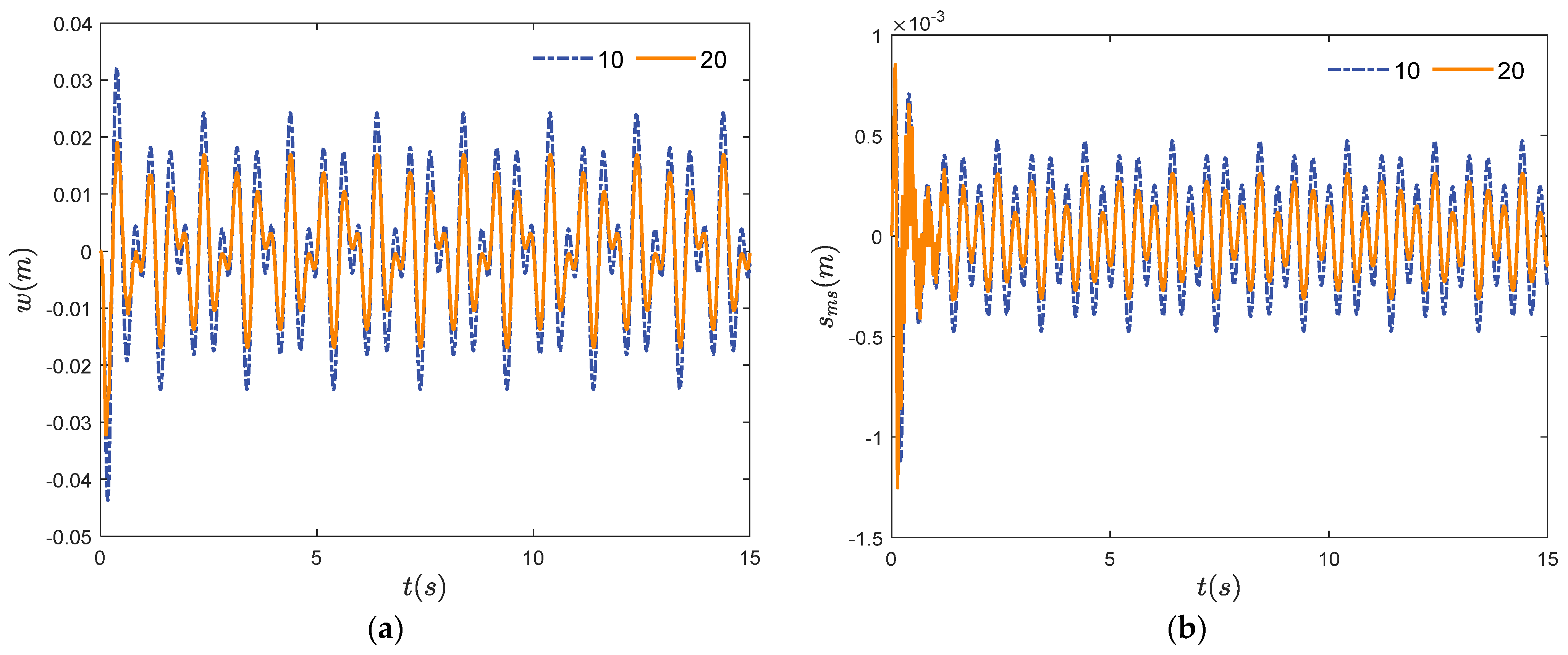
ADP Case 2: The ADP controller applies 20 sensors’ information. The number of hidden layer nodes and learning rates are set the same as ADP Case 1. The state and input weight matrices are and . The spatial time representation is shown in Figure 6.
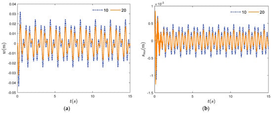
Figure 6.
Results of displacement. (a) Displacement of the structure’s free end for ADP control with 10 and 20 sensors; (b) sloshing displacement for ADP control with 10 and 20 sensors.
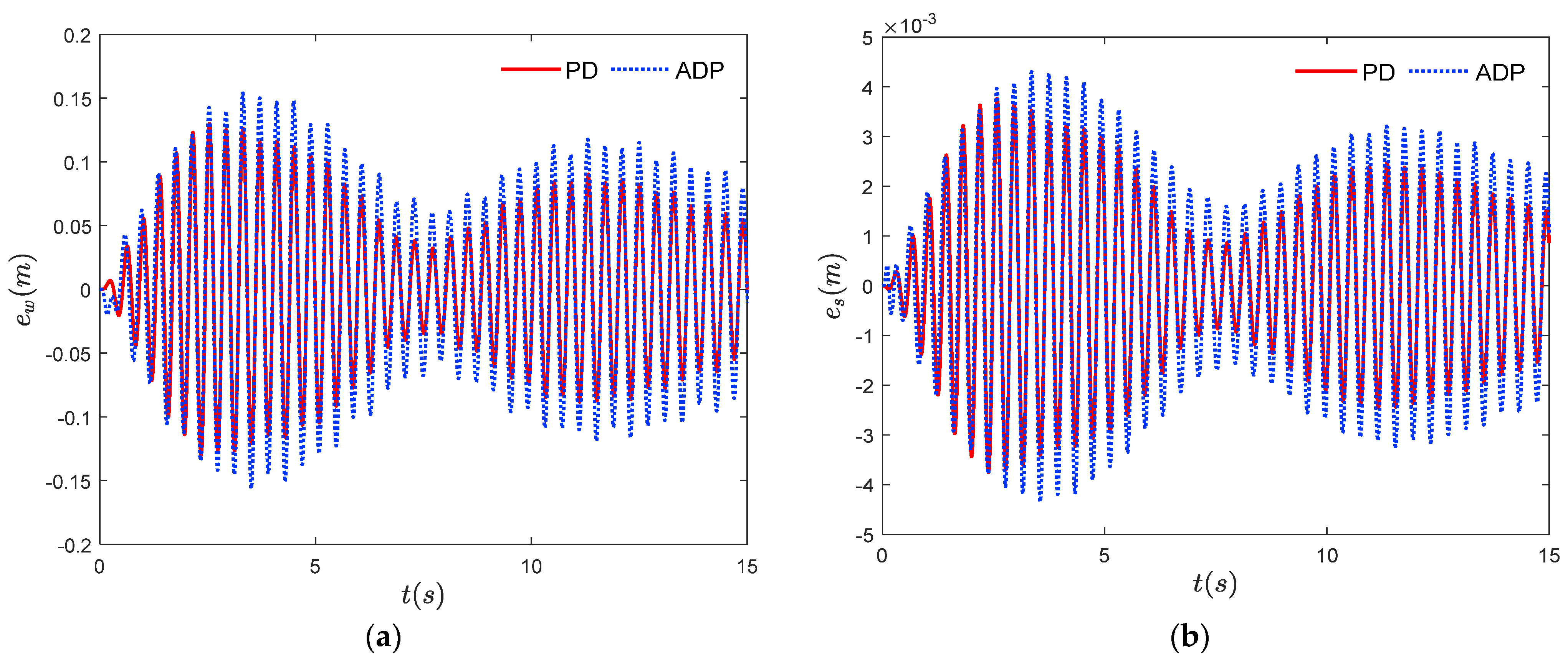
PD Case: For comparison, the spatial time representation of the displacement with the PD controller is shown in Figure 7. The PD controller is designed as , and the parameters are set as , .
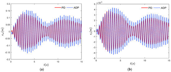
Figure 7.
Error results of displacement relative to free case. (a) Displacement of the structure’s free end in PD case and ADP case 1; (b) sloshing displacement in PD case and ADP case 1.
As shown in Figure 4a, it can be observed that there are significant vibrations along the structure subjected to the sinusoidal disturbance . In Figure 4b–d, both the ADP and PD controllers can suppress the vibration of the coupling systems when the system is subjected to external disturbance . Furthermore, it is evident that the displacement under ADP control is smaller than that under PD control.
For further analysis, the displacements of the structure’s free end and sloshing in the free case, PD case, and ADP case 1 are shown in Figure 5. The displacement errors (between PD case and free case, between ADP case 1 and free case) of the structure’s free end and sloshing are shown in Figure 7a,b. As illustrated in Figure 5a and Figure 7a, the ADP controller with 10 sensors and a PD controller can suppress the vibration at the small neighborhood of its equilibrium position. Moreover, the output position in ADP case 1 is smaller than that in the PD case. Similarly, Figure 5b and Figure 7b demonstrate that both the ADP controller with 10 sensors and the PD controller can suppress the sloshing in the tank subject to disturbance, with the ADP case 1 producing smaller sloshing displacement than the PD case. The simulation results in Figure 5 and Figure 7 indicate that the ADP method has better performance of elastic vibration and sloshing suppression in comparison to the PD controller.
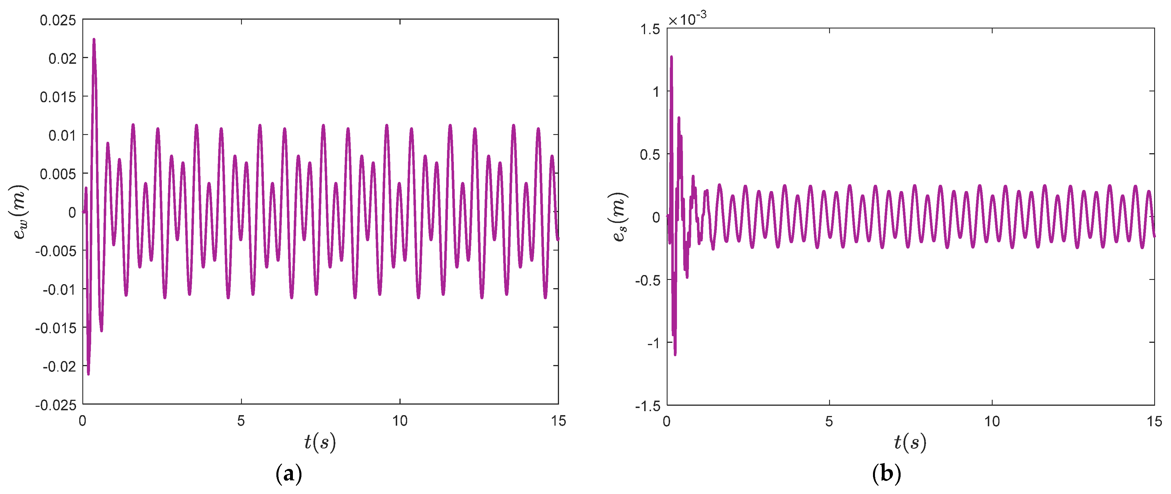
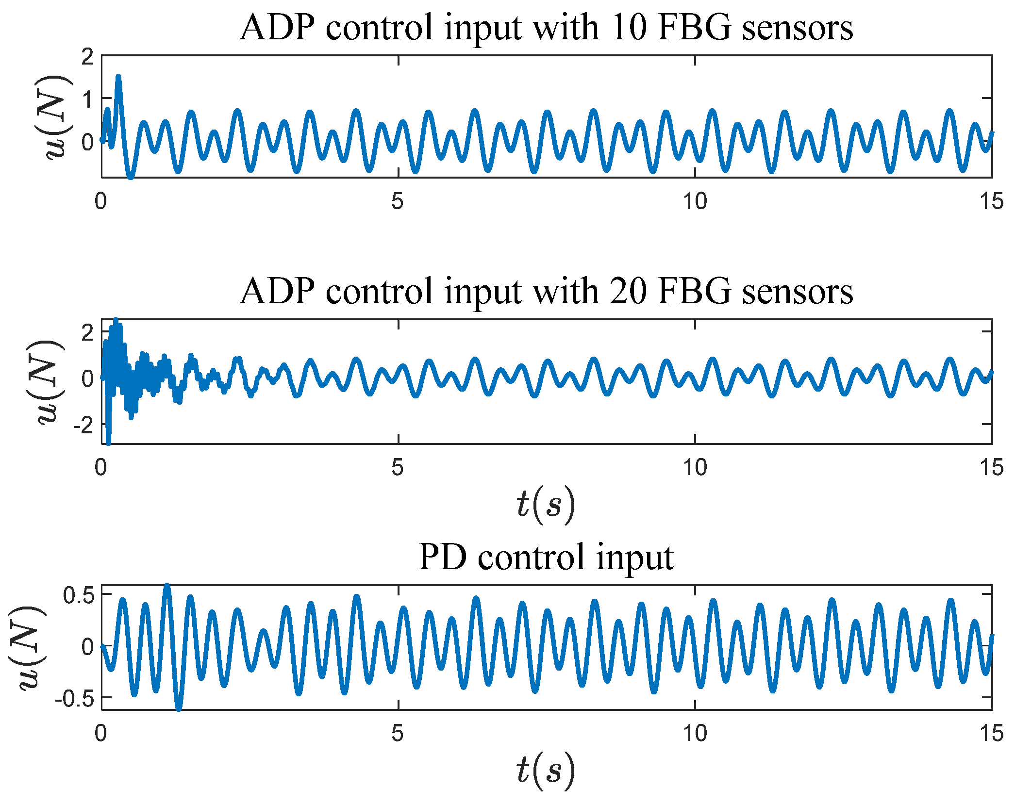
To analyze the performance of the ADP controller using varying numbers of sensors, the displacement of the structure’s free end and sloshing are shown in Figure 6a,b, respectively. The displacement errors of the structure’s free end and sloshing between ADP case 1 and ADP case 2 are shown in Figure 8a,b. We can observe that the displacement of the structure’s free end and sloshing in ADP case 2 is smaller than that in ADP case 1. As the amount of sensor information increases, the performance of the ADP controller becomes more effective. However, the displacement of sloshing and control input within 2 s changes drastically under ADP control using 20 sensors’ information. Finally, the ADP and PD control inputs are shown in Figure 9.
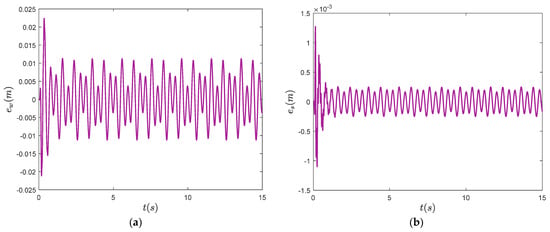
Figure 8.
Error results of displacement between ADP case 1 and ADP case 2. (a) Displacement of the structure’s free end; (b) sloshing displacement.
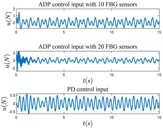
Figure 9.
ADP control inputs with 10 and 20 sensors and PD control input.
In conclusion, the simulation results have demonstrated the effectiveness of the ADP method in suppressing the elastic vibration and sloshing of the coupling system when disturbance is exerted. Compared with other methods, the designed ADP controller only requires partial strain information and does not need the motion parameters of the coupling system. Additionally, as the amount of sensor information applied increases, the performance of the ADP controller becomes more effective. However, the displacement of sloshing undergoes significant changes, which means that the selection of the appropriate number of sensors depends on the compromise between the final performance of the ADP control and the initial violent sloshing during control.
5. Conclusions
In this paper, the elastic vibration and sloshing suppression control problem is investigated via the ADP algorithm based on strain information measured from FBG. The controller is designed using the strain information measured by FBG, with its first-order derivative estimated by a tracking differentiator. The Euler–Bernoulli theory and spring-mass-damper equivalent mechanical model are employed to establish the flexible-sloshing coupling dynamic model. Additionally, the strain-based vibration dynamic model is derived through the relationship between the strain and the node displacement based on the FEM. Furthermore, the controller is designed based on ADHDP structure with neural networks. The main advantages of the proposed method can be concluded as follows:
- (1)
- The usages of the Euler–Bernoulli beam model and the spring-mass-damper equivalent model provide a simpler and more convenient way for constructing the flexible-sloshing coupling dynamic model.
- (2)
- The development of a strain-based vibration dynamic model facilitates the full utilization of FBG sensors’ strain information.
- (3)
- This controller can effectively suppress elastic vibration and sloshing with only partial strain information, eliminating the process of estimating the vibration motion parameters. The control strategy indicates important implications in engineering applications.
In the future, we will conduct further research on three-dimensional vibration suppression control and the control performance of different numbers of sensors.
Author Contributions
Conceptualization, D.Z.; methodology, C.K.; software, C.K.; validation, C.K. and D.Z.; formal analysis, C.K.; investigation, C.K.; resources, D.Z.; data curation, C.K.; writing—original draft preparation, C.K.; writing—review and editing, D.Z. and B.L.; visualization, C.K.; supervision, D.Z. and B.L.; project administration, D.Z. and B.L.; funding acquisition, D.Z. and B.L. All authors have read and agreed to the published version of the manuscript.
Funding
This research received no external funding.
Data Availability Statement
No new data were created or analyzed in this study. Data sharing is not applicable to this article.
Conflicts of Interest
The authors declare no conflict of interest.
References
- Guo, S.-S.; Kim, J. Some Recent Developments in the Vibration Control and Structure Health Monitoring. Actuators 2023, 12, 11. [Google Scholar] [CrossRef]
- He, G.; Cao, D. Dynamic Modeling and Attitude-Vibration Cooperative Control for a Large-Scale Flexible Spacecraft. Actuators 2023, 12, 167. [Google Scholar] [CrossRef]
- Dai, J.; Qin, Y.; Wang, C.; Zhu, J.; Zhu, J. Research on Stability Control Technology of Hazardous Chemical Tank Vehicles Based on Electromagnetic Semi-Active Suspension. Actuators 2023, 12, 333. [Google Scholar] [CrossRef]
- Su, W.; King, C.K.; Clark, S.R.; Griffin, E.D.; Suhey, J.D.; Wolf, M.G. Dynamic Beam Solutions for Real-Time Simulation and Control Development of Flexible Rockets. J. Spacecr. Rocket. 2017, 54, 403–416. [Google Scholar] [CrossRef]
- Peterson, L.D.; Crawley, E.F.; Hansman, R.J. Nonlinear fluid slosh coupled to the dynamics of a spacecraft. AIAA J. 1989, 27, 1230–1240. [Google Scholar] [CrossRef]
- Frosch, J.A.; Vallely, D.P. Saturn AS-501/S-IC flight control system design. J. Spacecr. Rocket. 1967, 4, 1003–1009. [Google Scholar] [CrossRef]
- Unruh, J.F.; Kana, D.D.; Dodge, F.T.; Fey, T.A. Digital data analysis techniques for extraction of slosh model parameters. J. Spacecr. Rocket. 1986, 23, 171–177. [Google Scholar] [CrossRef]
- Guo, N.; Yang, Z.; Wang, L.; Ouyang, Y.; Zhang, X. Dynamic model updating based on strain mode shape and natural frequency using hybrid pattern search technique. J. Sound Vib. 2018, 422, 112–130. [Google Scholar] [CrossRef]
- Mooij, E.; Gransden, D.I. The Effect of Sloshing on the Controllability of a Conventional Aeroelastic Launch Vehicle. In AIAA Scitech 2019 Forum; AIAA SciTech Forum; American Institute of Aeronautics and Astronautics: Reston, VA, USA, 2019. [Google Scholar]
- Panopoulou, A.; Roulias, D.; Loutas, T.H.; Kostopoulos, V. Health Monitoring of Aerospace Structures Using Fibre Bragg Gratings Combined with Advanced Signal Processing and Pattern Recognition Techniques. Strain 2012, 48, 267–277. [Google Scholar] [CrossRef]
- Chuang, K.; Lin, S.; Ma, C.; Wu, R. Application of a Fiber Bragg Grating-Based Sensing System on Investigating Dynamic Behaviors of a Cantilever Beam Under Impact or Moving Mass Loadings. IEEE Sens. J. 2013, 13, 389–399. [Google Scholar] [CrossRef]
- Kong, C.; Zhao, D.; Zhang, J.; Liang, B. Real-Time Virtual Sensing for Dynamic Vibration of Flexible Structure via Fiber Bragg Grating Sensors. IEEE Sens. J. 2022, 22, 21706–21718. [Google Scholar] [CrossRef]
- Abramson, H.N. The Dynamic Behavior of Liquids in Moving Containers With Applications to Space Vehicle Technology; NASA: Washington, DC, USA, 1966.
- Su, N.; Bian, J.; Peng, S.; Chen, Z.; Xia, Y. Balancing static and dynamic performances of TMD with negative stiffness. Int. J. Mech. Sci. 2023, 243, 108068. [Google Scholar] [CrossRef]
- Chen, Z.; Chen, Z.; Wei, Y. Quasi-Zero Stiffness-Based Synchronous Vibration Isolation and Energy Harvesting: A Comprehensive Review. Energies 2022, 15, 7066. [Google Scholar] [CrossRef]
- Kapasakalis, K.A.; Antoniadis, I.A.; Sapountzakis, E.J. Performance assessment of the KDamper as a seismic Absorption Base. Struct. Control. Health Monit. 2020, 27, e2482. [Google Scholar] [CrossRef]
- Kapasakalis, K.A.; Antoniadis, I.A.; Sapountzakis, E.J. Constrained optimal design of seismic base absorbers based on an extended KDamper concept. Eng. Struct. 2021, 226, 111312. [Google Scholar] [CrossRef]
- Wang, J.; Liu, J.; Li, Y.; Chen, C.L.P.; Liu, Z.; Li, F. Prescribed Time Fuzzy Adaptive Consensus Control for Multiagent Systems With Dead-Zone Input and Sensor Faults. IEEE Trans. Autom. Sci. Eng. 2023, 21, 1–12. [Google Scholar] [CrossRef]
- Wang, J.; Gong, Q.; Huang, K.; Liu, Z.; Chen, C.L.P.; Liu, J. Event-Triggered Prescribed Settling Time Consensus Compensation Control for a Class of Uncertain Nonlinear Systems With Actuator Failures. IEEE Trans. Neural Networks Learn. Syst. 2023, 34, 5590–5600. [Google Scholar] [CrossRef]
- Wang, J.; Wang, C.; Liu, Z.; Chen, C.L.P.; Zhang, C. Practical Fixed-Time Adaptive ERBFNNs Event-Triggered Control for Uncertain Nonlinear Systems With Dead-Zone Constraint. IEEE Trans. Syst. Man Cybern. Syst. 2023, 54, 1–10. [Google Scholar] [CrossRef]
- Goh, C.J.; Caughey, T.K. On the stability problem caused by finite actuator dynamics in the collocated control of large space structures. Int. J. Control 1985, 41, 787–802. [Google Scholar] [CrossRef]
- Mahmoodi, S.N.; Ahmadian, M. Active Vibration Control With Modified Positive Position Feedback. J. Dyn. Syst. Meas. Control 2009, 131, 041002. [Google Scholar] [CrossRef]
- Lieven, N.A.J.; Ewins, D.J.; Inman, D.J. Active modal control for smart structures. Philos. Trans. R. Soc. London. Ser. A Math. Phys. Eng. Sci. 2001, 359, 205–219. [Google Scholar] [CrossRef]
- Baz, A.; Poh, S. Performance of an active control system with piezoelectric actuators. J. Sound Vib. 1988, 126, 327–343. [Google Scholar] [CrossRef]
- Wang, Z.; Wu, W.; Görges, D.; Lou, X. Sliding mode vibration control of an Euler–Bernoulli beam with unknown external disturbances. Nonlinear Dyn. 2022, 110, 1393–1404. [Google Scholar] [CrossRef]
- He, W.; Ge, S.S. Vibration Control of a Flexible Beam With Output Constraint. IEEE Trans. Ind. Electron. 2015, 62, 5023–5030. [Google Scholar] [CrossRef]
- Ma, Y.; Lou, X.; Miller, T.; Wu, W. Fault-Tolerant Boundary Control of an Euler–Bernoulli Beam Subject to Output Constraint. IEEE Trans. Syst. Man Cybern. Syst. 2023, 53, 4753–4763. [Google Scholar] [CrossRef]
- Feng, Y.; Liu, Z. Adaptive Vibration Iterative Learning Control of an Euler–Bernoulli Beam System With Input Saturation. IEEE Trans. Syst. Man Cybern. Syst. 2023, 53, 2469–2477. [Google Scholar] [CrossRef]
- Mirafzal, S.H.; Khorasani, A.M.; Ghasemi, A.H. Optimizing time delay feedback for active vibration control of a cantilever beam using a genetic algorithm. J. Vib. Control 2015, 22, 4047–4061. [Google Scholar] [CrossRef]
- Lin, J.; Chao, W.S. Vibration Suppression Control of Beam-cart System with Piezoelectric Transducers by Decomposed Parallel Adaptive Neuro-fuzzy Control. J. Vib. Control 2009, 15, 1885–1906. [Google Scholar] [CrossRef]
- He, W.; Gao, H.; Zhou, C.; Yang, C.; Li, Z. Reinforcement Learning Control of a Flexible Two-Link Manipulator: An Experimental Investigation. IEEE Trans. Syst. Man Cybern. Syst. 2021, 51, 7326–7336. [Google Scholar] [CrossRef]
- Qiu, Z.-c.; Yang, Y.; Zhang, X.-m. Reinforcement learning vibration control of a multi-flexible beam coupling system. Aerosp. Sci. Technol. 2022, 129, 107801. [Google Scholar] [CrossRef]
- Wang, F.Y.; Zhang, H.; Liu, D. Adaptive Dynamic Programming: An Introduction. IEEE Comput. Intell. Mag. 2009, 4, 39–47. [Google Scholar] [CrossRef]
- Jiang, H. Real Time Mode Sensing and Attitude Control of Flexible Launch Vehicle with Fiber Bragg Grating Sensor Array; Florida Institute of Technology: Melbourne, FL, USA, 2011. [Google Scholar]
- Orr, J.S. Robust Autopilot Design for Lunar Spacecraft Powered Descent Using High Order Sliding Mode Control; The University of Alabama in Huntsville: Huntsville, AL, USA, 2009. [Google Scholar]
- Kwon, Y.W.; Bang, H. The Finite Element Method Using MATLAB; London CRC Press: Boca Raton, FL, USA, 2000. [Google Scholar]
- Ibrahim, R.A. Liquid Sloshing Dynamics: Theory and Applications; Cambridge University Press: New York, NY, USA, 2005. [Google Scholar]
- Dodge, F.T. Analytical Representation of Lateral Sloshing by Equivalent Mechanical Models; NASA Special Publication: Washington, DC, USA, 1966; p. 199.
- Song, X.; Liang, D. Dynamic displacement prediction of beam structures using fiber bragg grating sensors. Optik 2018, 158, 1410–1416. [Google Scholar] [CrossRef]
- Wu, S.Q.; Zhou, J.X.; Rui, S.; Fei, Q.G. Reformulation of elemental modal strain energy method based on strain modes for structural damage detection. Adv. Struct. Eng. 2017, 20, 896–905. [Google Scholar] [CrossRef]
- Zhao, D.-J.; Wang, Y.-J.; Liu, L.; Wang, Z.-S. Robust Fault-Tolerant Control of Launch Vehicle Via GPI Observer and Integral Sliding Mode Control. Asian J. Control 2013, 15, 614–623. [Google Scholar] [CrossRef]
- Zhong, X.; He, H. An Event-Triggered ADP Control Approach for Continuous-Time System With Unknown Internal States. IEEE Trans. Cybern. 2017, 47, 683–694. [Google Scholar] [CrossRef]
- Igelnik, B.; Yoh-Han, P. Stochastic choice of basis functions in adaptive function approximation and the functional-link net. IEEE Trans. Neural Netw. 1995, 6, 1320–1329. [Google Scholar] [CrossRef]
- Liu, F.; Sun, J.; Si, J.; Guo, W.; Mei, S. A boundedness result for the direct heuristic dynamic programming. Neural Netw. 2012, 32, 229–235. [Google Scholar] [CrossRef]
- Khalil, H.K. Nonlinear Systems; Prentice Hall: Upper Saddle River, NJ, USA, 2002. [Google Scholar]


Disclaimer/Publisher’s Note: The statements, opinions and data contained in all publications are solely those of the individual author(s) and contributor(s) and not of MDPI and/or the editor(s). MDPI and/or the editor(s) disclaim responsibility for any injury to people or property resulting from any ideas, methods, instructions or products referred to in the content. |
© 2023 by the authors. Licensee MDPI, Basel, Switzerland. This article is an open access article distributed under the terms and conditions of the Creative Commons Attribution (CC BY) license (https://creativecommons.org/licenses/by/4.0/).