Path Tracking Control of Intelligent Vehicles Considering Multi-Nonlinear Characteristics for Dual-Motor Autonomous Steering System

Abstract

In the path tracking control of intelligent vehicles, the traditional linear control method is prone to high tracking errors for uncertain parameters of the steering transmission system and road conditions. Therefore, considering the mechanical friction in the dual-motor autonomous steering system and the nonlinearity of tires, this paper proposes a path tracking control strategy of intelligent vehicles for the dual-motor autonomous steering system that considers nonlinear characteristics. First, a dual-motor autonomous steering system considering mechanical friction and the variation of tire cornering stiffness under different tire–road friction coefficients was established based on the structure of an autonomous steering system. Second, a tire–road friction coefficient estimator was designed based on a PSO-LSTM neural network. The tire cornering stiffness under different tire–road friction coefficients was estimated through the recursive least-square algorithm. Then, the control strategy of the dual-motor autonomous steering system was designed by combining the LQR path tracking controller with the adaptive sliding mode control strategy based on field-oriented control. Here, mechanical friction and the variation of tire cornering stiffness were considered. Finally, simulation and HiL tests validated the method proposed in this paper. The results show that the proposed control strategy significantly improves the tracking accuracy and performance of the dual-motor autonomous steering system for intelligent vehicles.

1. Introduction

With the rapid development of automatic driving technology in recent years, researchers have actively contributed to autonomous steering systems [1,2]. When compared to the conventional steering system, the autonomous steering system directly controls the steering actuator through electrical signals. Alternatively, the motor drives the steering transmission mechanism to track the target angle, further improving the mobility of vehicles. Autonomous steering systems can also facilitate advanced active safety technologies, such as lane keeping, obstacle avoidance, lane changing and automatic parking [3,4,5]. As research advanced, the dual-motor autonomous steering system was developed to fulfill the safety requirements of intelligent vehicles at level two and above [6].

The dual-motor autonomous steering system redundantly backups the controller and steering motors, allowing coordinated control of the dual motors under extreme operating conditions, lessening the load on the controller and enhancing active safety of vehicles [7,8,9]. In the event of a single motor failure, the dual-motor autonomous steering system reconfigures the operating mode of the system to maintain a certain level of steering functionality, avoiding steering failure when a single motor fails to work. The dual-motor autonomous steering system has a high level of reliability and safety through redundant design and fault-tolerant mechanism [10,11,12].

In addition to reliability and safety, there is also a high demand for path tracking accuracy in the evaluation criteria of autonomous steering systems for its performance. Li et al. [13] proposed a model predictive path tracking control strategy based on tire state stiffness prediction. The nonlinear model predictive controller and linear model for time-varying path tracking control were proposed to improve the path tracking performance of intelligent vehicles under extreme conditions. Peng et al. [14] proposed a robust MPC theory with a finite time range to reduce the impact on tracking accuracy caused by the uncertainty of tire cornering stiffness. The literature considered the variation of tire cornering stiffness during trajectory tracking. However, the accuracy of the estimated tire–road friction coefficient also has a significant impact on the estimation outcomes of the tire cornering stiffness. Hao et al. [15] proposed a tire–road friction coefficient identification approach based on the RNN. However, due to the gradient disappearance of the RNN model, it could not learn the long-term dependence relationship of the time-series data. Yu et al. [16] established a BP neural network-based estimator of the tire–road friction coefficient with consideration of the pavement roughness and proposed a prediction model. Ribeiro et al. [17] proposed a tire–road friction coefficient estimation method based on a time-delay neural network using the tire lateral force data. Furthermore, the existence of strong nonlinearity to tire–road friction coefficient estimation needs to be addressed by a data-driven approach. However, the difference in network models will affect the accuracy of tire–road friction coefficient estimation.

The sliding mode control technique has been widely used to improve the tracking performance of the nonlinear control system due to its strong robustness to uncertainty. Sun et al. [18] proposed an adaptive fast non-singular terminal sliding mode controller to provide accurate and stable steering performance. However, the controller regards self-aligning torque and friction torque as external disturbance and lacks a specific dynamic model. Kazemi et al. [19] proposed a nonlinear adaptive sliding mode control algorithm to improve the vehicle handling performance through the steering-by-wire system. Although an adaptive sliding mode algorithm was theoretically proposed to estimate the tire cornering stiffness, the adaptive scheme was difficult to apply to vehicles with large load variation. Li et al. [20] proposed an adaptive higher-order sliding mode control method to overcome uncertainty in the unknown dynamic model. However, the uncertainty boundaries were difficult to determine when the tire–road friction coefficient fluctuated significantly. Wang et al. [21] proposed an adaptive fuzzy neural network to approximate the unknown dynamic of the system. The control strategy eliminates the need for friction torque and steering self-aligning torque. However, the algorithm’s accuracy is constrained by the difficulty of acquiring tire parameters and monitoring nonlinear components. In conclusion, the current research on the tracking accuracy of the autonomous steering system only sets a simple dynamic model, ignoring the influence of nonlinearity on path tracking control. Therefore, in order to solve the problem of large tracking errors caused by the friction of the mechanical structures, the nonlinearity of tires, the uncertainty parameters of steering transmission system and the road conditions, a control strategy for the dual-motor autonomous steering system considering the multi-nonlinear characteristics is proposed in this paper.

The main contributions of this paper are as follows: (1) Considering the uncertain parameters and mechanical friction of the autonomous steering system, the LuGre friction model was applied for friction compensation control to improve the tracking performance; (2) The tire–road friction coefficient estimator based on PSO-LSTM was used to calculate the tire–road friction coefficient for the advantage of neural networks to deal with nonlinear problems. The tire cornering stiffness was estimated through the recursive least-square algorithm for its high accuracy; (3) The adaptive sliding mode control strategy based on field-oriented control considers the mechanical friction of the transmission mechanism and the variation of tire cornering stiffness to improve the tracking accuracy of the path tracking control under multi-nonlinear characteristics; (4) The proposed control strategy was verified through the simulation and the HiL test. Through the estimation of vehicle state parameters and the design of control strategy considering the anti-disturbance ability, the tracking accuracy can be improved from a practice perspective.

The rest of the paper is organized as follows: the self-aligning torque model is presented in Section 2. The creation of the PSO-LSTM neural network data set and the optimization of the network structure are presented in Section 3. An LQR path tracking control strategy and a control strategy for the dual-motor autonomous steering system considering mechanical friction and the variation of tire cornering stiffness are designed in Section 4. Simulation results are given in Section 5 and Section 6 provides the HiL results. Lastly, the conclusions are drawn in Section 7.

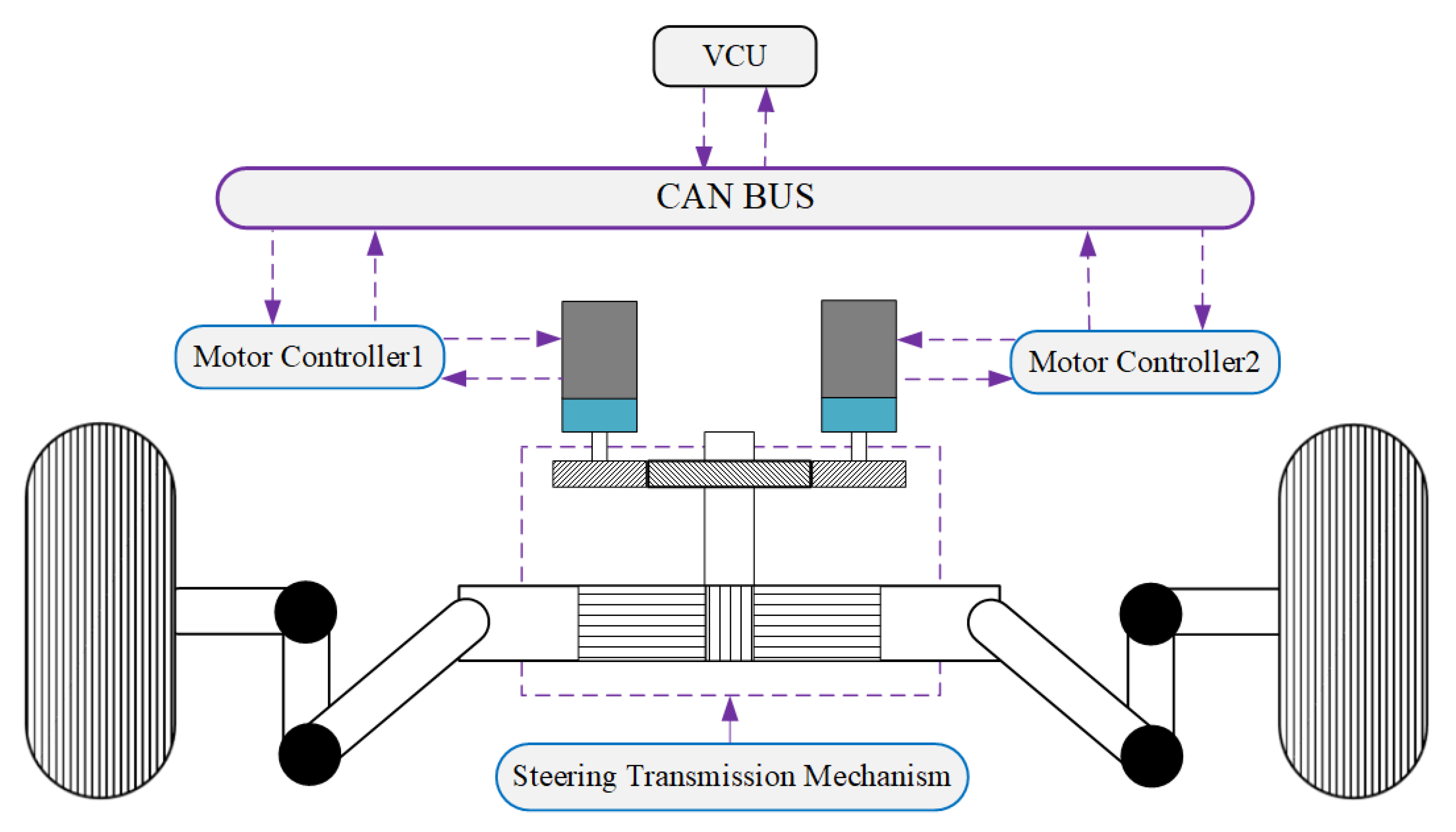
2. Autonomous Steering System

The structure of the dual-motor autonomous steering system is proposed as follows. Combined with the mechanical friction of the autonomous steering system, the dynamic model of the dual-motor autonomous steering system considering mechanical friction is established. In addition, the self-aligning torque model is established to obtain the effect it brings to the tire cornering stiffness when the tire–road friction coefficient changes.

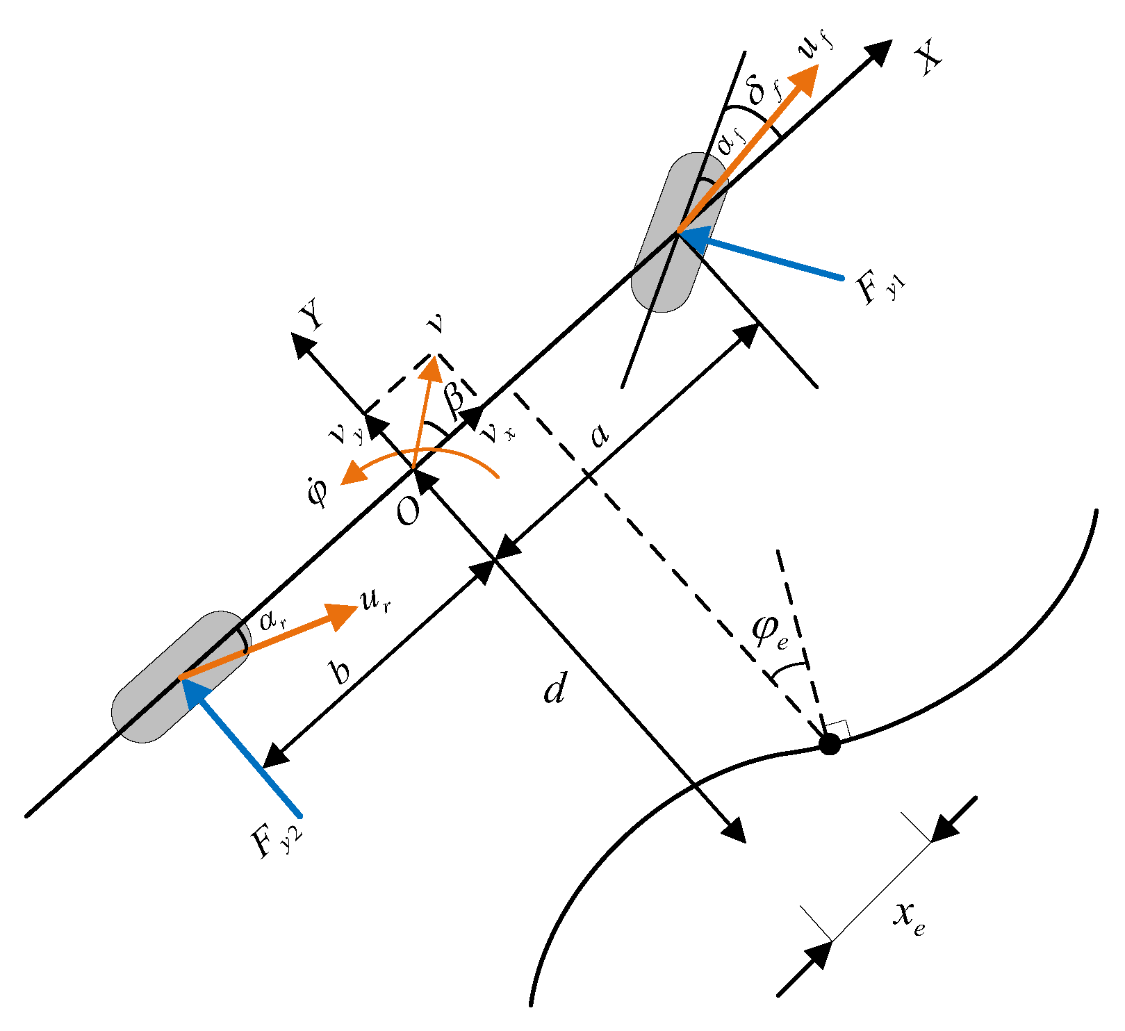
2.1. Model for Autonomous Steering System

A dual-motor autonomous steering system consists of a path tracking controller, two motor controllers, two steering motors and the steering transmission mechanism. The structure of the dual-motor autonomous steering system is shown in Figure 1. Based on the information sent from the upper controller, the path tracking controller calculates the target front wheel angle at the current moment. The motor controllers then receive the signal of the target front wheel angle and drive the steering motors to achieve the target front wheel angle through the steering transmission mechanism.

According to the arrangement of the steering motors, two steering motors are arranged on both sides of the steering shaft, and the equivalent dynamic equation can be expressed as

$$T_{\mathrm{sm}}=J_{\mathrm{s}m1}{\ddot{\theta }}_{\mathrm{s}m1}+B_{\mathrm{s}m1}{\dot{\theta }}_{\mathrm{s}m1}+J_{\mathrm{s}m2}{\ddot{\theta }}_{sm2}+B_{sm2}{\dot{\theta }}_{sm2}+{\tau }_{w2m},$$

(1)

where $J_{sm1}$ and $J_{sm2}$ are inertias of steering motors, respectively, $B_{sm1}$ and $B_{sm2}$ are viscous damping coefficients of steering motors respectively, ${\theta }_{sm1}$ and ${\theta }_{sm2}$ are rotation angles of the motors, respectively, ${\tau }_{w2m}$ is the equivalent torque of the wheel acting on the output shaft of the steering motors, $T_{sm}$ is the total torque of the steering motors.

The aforementioned equation can only represent the dynamic equations of the dual-motor autonomous steering system under ideal conditions. However, this equation does not consider the influence of the mechanical friction of the gearbox, steering gear and steering rack in the steering transmission mechanism. In the actual dual-motor autonomous steering system, the frictional torque weakens the steering assist torque, worsens the assisting effect, and affects the dynamic characteristics of the steering system. In order to lessen and minimize the effect of friction on the steering transmission mechanism. The LuGre friction model [22] uses the concept of bristles, which regards the contact surface of the system equivalently to many elastic bristles with random behavior and generates friction torque due to the deformation of bristles. The formula is expressed as follows:

$$\left\{\begin{array}{c}{T}_f={\sigma }_0\zeta +{\sigma }_1\frac{d\zeta }{dt}\hfill \\ \frac{d\zeta }{dt}=\dot{\theta }-\frac{|\dot{\theta }|}{g\left(\dot{\theta }\right)}\zeta ,\hfill \end{array}\right.$$

(2)

where $T_f$ is the friction compensation torque, $\dot{\theta }$ is the relative angular velocity of the contact surface, ${\sigma }_0$ is the stiffness coefficient, ${\sigma }_1$ is the damping coefficient, and $\zeta$ is the average deformation of the bristles. The function $g\left(\dot{\theta }\right)$ is higher than zero and its characteristics include asymmetry, which do not depend on material, lubrication or temperature. Moreover, they increase monotonically with the angular velocity.

The LuGre friction model is integrated with the aforementioned dynamics equations to obtain dynamic equations of the dual-motor autonomous steering system that considers mechanical friction, which is expressed as follows:

$$T_{\mathrm{sm}}+T_f=J_{\mathrm{s}m1}{\ddot{\theta }}_{\mathrm{s}m1}+B_{\mathrm{s}m1}{\dot{\theta }}_{\mathrm{s}m1}+J_{\mathrm{s}m2}{\ddot{\theta }}_{sm2}+B_{sm2}{\dot{\theta }}_{sm2}+{\tau }_{w2m}.$$

(3)

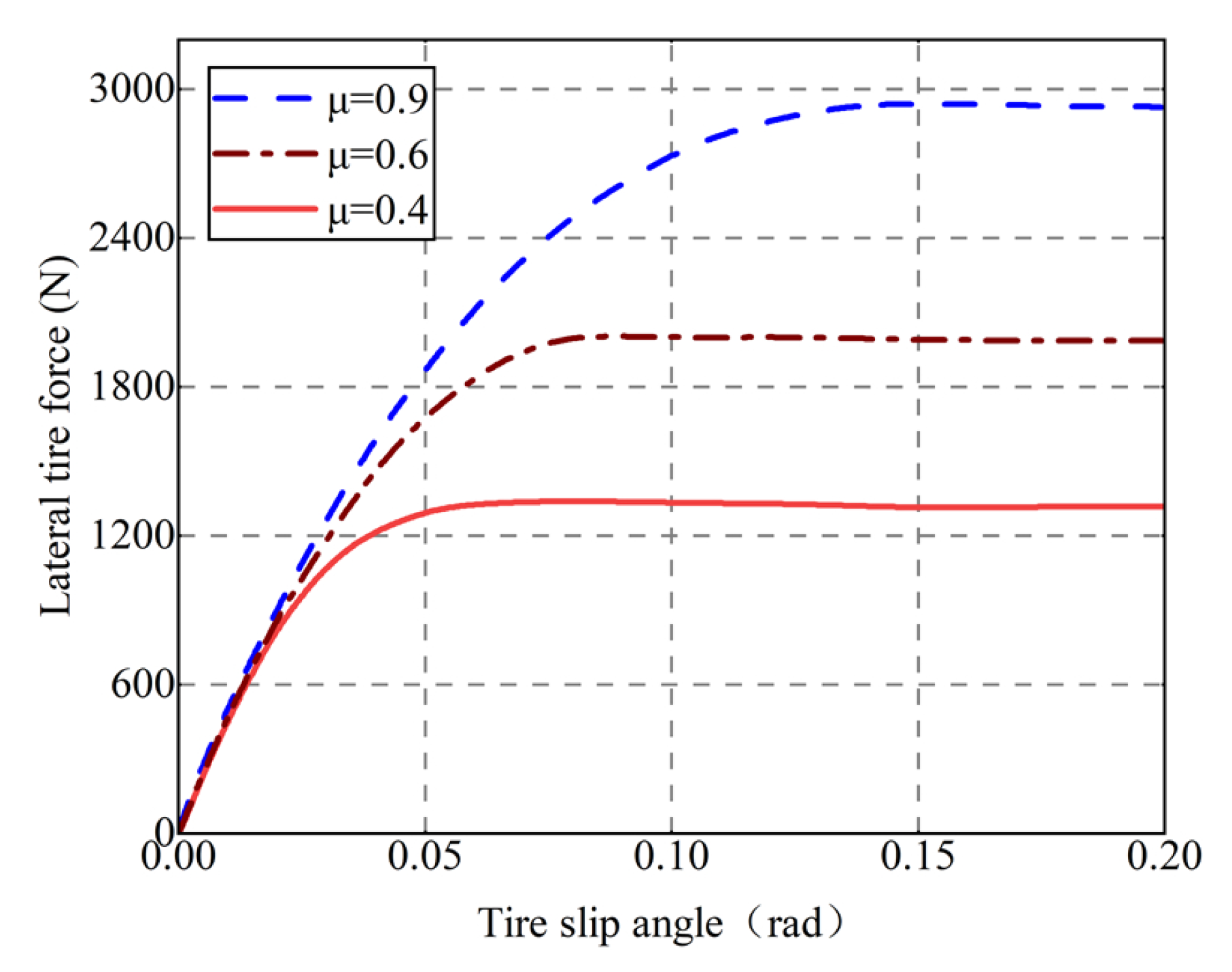
2.2. Model for Self-Aligning Torque

The self-aligning torque is impacted by changes in tire cornering stiffness under different tire–road friction coefficients. A self-aligning torque model is established to assess the equivalent disturbance amount of the self-aligning torque to the steering system. The self-aligning torque that considers the lateral force of the tire can be expressed as

$${\tau }_e=(l_c+l_p)·F_{yf},$$

(4)

where $l_c$ is the mechanical trail, $l_p$ is the pneumatic trail, and $F_{yf}$ is the tire lateral force. The tire’s size, structure, and driving conditions of the vehicle affect the tire cornering stiffness. In addition, a significant factor affecting tire cornering stiffness is the tire–road friction coefficient. Figure 2 shows the tire slip characteristic curves under different tire–road friction coefficients. The tire lateral force has an approximately linear relationship with the tire slip angle, which can be expressed as

$$F_{yf}=C_f·{\alpha }_f,$$

(5)

where $C_f$ is the tire cornering stiffness.

It can be seen that the tire lateral force is linearly related to the tire slip angle when the tire slip angle is approximately zero.

Assuming that the vehicle slip angle is approximately zero, the tire slip angle is as follows:

$${\alpha }_f=\beta +\frac{l_f{\omega }_r}{u}-{\delta }_f,$$

(6)

where $\beta$ is the sideslip angle of the vehicle, ${\omega }_r$ is the yaw rate, $l_f$ is the distance from the center of mass to the front axle, u is the speed of the vehicle, and ${\delta }_f$ is the front wheel angle. The expression for the self-aligning torque is obtained by substituting Equation (6) in Equation (4).

$${\tau }_e=(l_c+l_p)·(\beta +\frac{l_f{\omega }_r}{u}-{\delta }_f)·C_f.$$

(7)

Assuming the ratio of the steering motor output shaft to the steering front wheel is $\eta$, and self-aligning torque equivalent to the torque acting on the output shaft of the steering motors can be expressed as

$${\tau }_{w2m}=\frac{{\tau }_e}{\eta }=\frac{(l_c+l_p)·(\beta +\frac{l_f{\omega }_r}{u}-{\delta }_f)·C_f}{\eta }.$$

(8)

The steady-state yaw rate ${\omega }_{rss}$ and steady-state sideslip angle ${\beta }_{ss}$ can be derived by using the bicycle model [23]. The yaw rate and sideslip angle in steady state can be obtained by replacing ${\dot{\omega }}_r$ and $\dot{\beta }$ with zero. The steady-equation can be expressed as

$$\left\{\begin{array}{c}{\omega }_{rss}=\frac{v_x}{(l_f+l_r)-\frac{m{v}_x^2(l_r{C}_r-l_f{C}_f)}{2(l_f+l_r)C_f{C}_r}}·{\delta }_f\hfill \\ {\beta }_{ss}=\frac{l_f-\frac{l_{f}m{v}_x^2}{2(l_f+l_r)C_r}}{(l_f+l_r)+\frac{m{v}_x^2(l_r{C}_r-l_f{C}_f)}{2(l_f+l_r)C_f{C}_r}}·{\delta }_f.\hfill \end{array}\right.$$

(9)

By substituting Equation (9) for Equation (8), the self-aligning torque considering the variation of tire cornering stiffness can be expressed as

$${\tau }_{w2m}=\frac{m{v}_x^2{l}_r{C}_f\left(\mu \right)C_r\left(\mu \right)}{2L^2{C}_f\left(\mu \right)C_r\left(\mu \right)-m{v}_x^2(l_f{C}_f\left(\mu \right)-l_r{C}_r\left(\mu \right))}·\frac{{\delta }_f(l_p+l_c)}{\eta },$$

(10)

where the tire cornering stiffness of front wheels and rear wheels considering the tire–road friction coefficient $\mu$ are $C_f\left(\mu \right)$ and $C_r\left(\mu \right)$, respectively.

By combining Equations (3) and (10), the dynamic equation of the dual-motor autonomous steering system considering mechanical friction and the variation of tire cornering stiffness can be expressed as

$$J_{sm}{\ddot{\theta }}_{sm}+B_{sm}{\dot{\theta }}_{sm}+{\tau }_{w2m}=K_{e}i+T_f,$$

(11)

where $J_{sm}$ is the equivalent rotational inertia of steering motors, $B_{sm}$ is the equivalent viscous friction coefficient of steering motors, ${\theta }_{sm}$ is the equivalent rotation angle of steering motors, $K_e$ is the torque coefficient of steering motors and i is the equivalent current.

3. Estimation of the Tire Cornering Stiffness

In order to estimate the variation of tire cornering stiffness, enhancing the accuracy of estimation under different tire–road friction coefficients to improve the adaptability of the dual-motor autonomous steering system on different road surfaces, a tire–road friction coefficient estimator based on PSO-LSTM and a tire cornering stiffness estimation method are proposed in this section.

3.1. Data Establishment

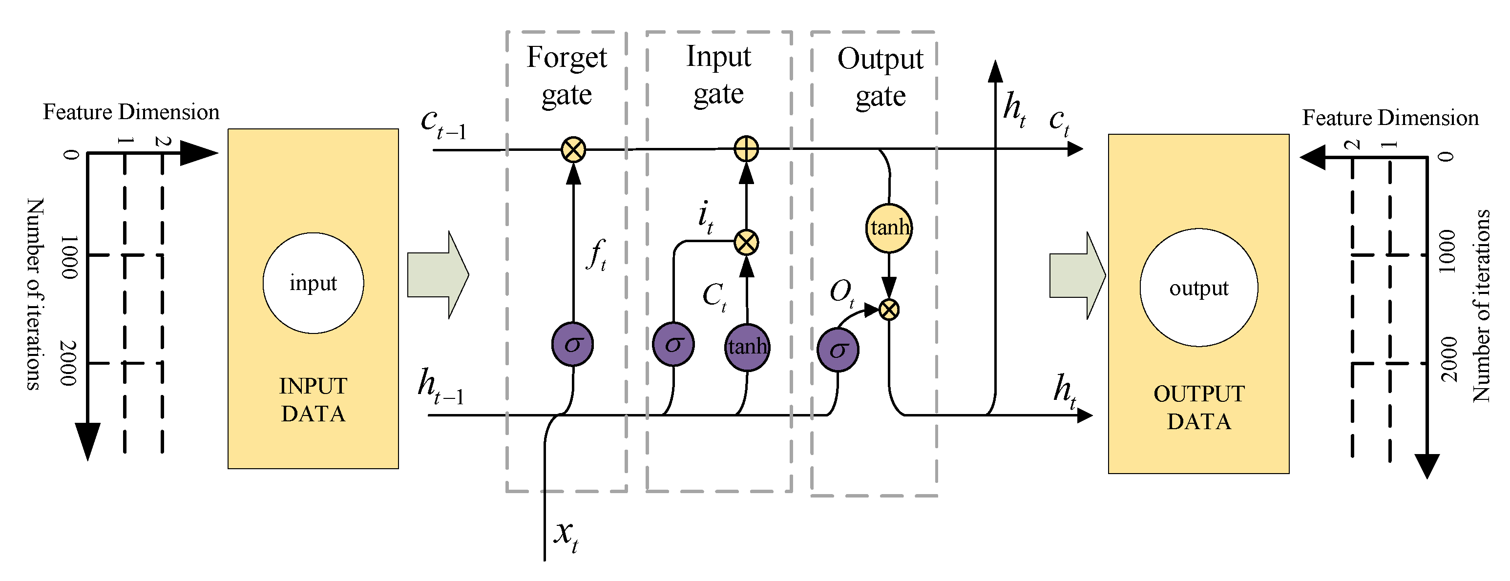
The driving conditions in the real driving process are very complex. Hence, the vehicle dynamics’ parameters must be collected under multiple driving conditions to make the estimated tire–road friction coefficients as close to the real condition as possible. Data were collected by using a joint simulation of the dual-motor autonomous steering system built in Matlab/Simulink and the vehicle dynamic software CarSim. Data collection included important vehicle dynamic parameters, such as: yaw rate ${\omega }_{\mathrm{r}}$, longitudinal vehicle velocity $v_x$, vehicle sideslip angle $\beta$, tire sideslip angle ${\alpha }_{f1}$ and ${\alpha }_{f2}$ of two front wheels, and yaw rate gain ${\omega }_{\mathrm{r}}/{\delta }_f$. The collected driving conditions are shown in

Table 1. Dataset collection conditions.

Driving Condition	Range of Velocity (km/h)	Range of Tire–Road Friction Coefficient
Single lane change of left turn	20∼100	0.3∼0.9
Single lane change of right turn	20∼100	0.3∼0.9
Double lane change of left turn	30∼80	0.3∼0.9
Double lane change of right turn	30∼80	0.3∼0.9
Straight ahead	20∼120	0.2∼1.0
Sine input	20∼60	0.4∼1.0
Constant circle steering	20∼60	0.4∼1.0
Step input	20∼80	0.3∼1.0

. Since the focus of this paper is on the effect of the tire–road friction coefficient related to tire cornering stiffness, the same vehicle type was used for data collection. The vehicle speed and tire–road friction coefficient were also set during data collection, with vehicle speed interval being 10 km/h and the tire–road friction coefficient interval being 0.1.

3.2. LSTM Model

The long short-term memory neural network (LSTM) [24,25,26] can save the unit state information C at the previous moment and control the proportion of flowing information. As a result, the LSTM is ideal for capturing time series features, where $x_t$ is the current input, $h_{t-1}$ is the previous moment input, $h_t$ is the current output, $C_t$ is the current state value, and $C_{t-1}$ is the state value of the previous time. The structure of the LSTM is illustrated in Figure 3.

The forgetting gate reads $h_{t-1}$, $x_t$ and exports a number between 0 and 1 through activation function $Sigmoid$, which determines the extent of information it forgets. The formula is expressed as

$$f_t=\sigma (W_f·[h_{t-1},x_t]+b_f).$$

(12)

The input gate determines the number of new messages to be added to the current period, Equation (13) determines the messages to be updated, and Equation (14) alternatively updates the messages through the activation function $\tanh$.

$$i_t=\sigma (W_i·[h_{t-1},x_t]+b_i)$$

(13)

$$\widetilde{C_t}=tanh(W_c·[h_{t-1},x_t]+b_c).$$

(14)

Consequently, the information of the new cell is updated by the forget gate and the input gate, which is expressed as

$$C_t=f_t\times C_{t-1}+i_t\times \widetilde{C_t}.$$

(15)

The output gate is determined by $O_t$, deciding which part of the cell state will be output. Then, the output of the network is obtained by processing the activation function $\tanh$.

$$O_t=\sigma (W_o[h_{t-1},x_t]+b_o)$$

(16)

$$h_t=O_t\times tanh\left(C_t\right),$$

(17)

where b is the bias vector; $f_t$ is the output of the neuron in the forgetting gate; W is the weight matrix; $\widetilde{C_t}$ is the candidate value during calculation; $i_t$ is the output of the neuron in the LSTM input gate; $O_t$ is the output of the neuron in the LSTM output gate.

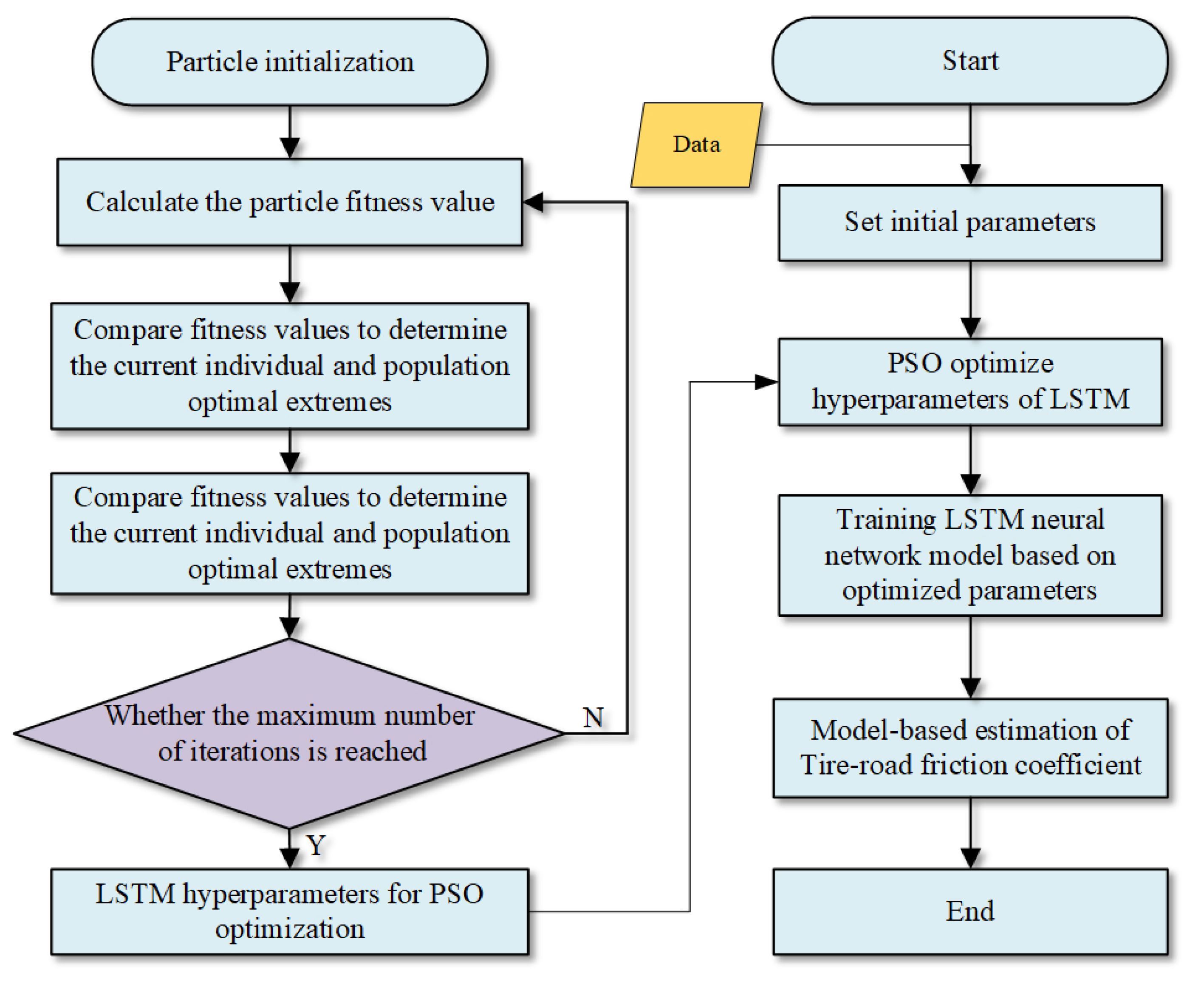
3.3. Establishment of the PSO-LSTM Model

The vehicle dynamics parameters collected in the data set in this paper are all time-series data. Even though the LSTM neural network has excellent time-series data processing capabilities, the choice of hyperparameters in the LSTM model can have a very significant impact on the model’s performance in predicting outcomes. Considering that the PSO algorithm [27,28] has certain advantages in dealing with multivariate optimization problems, the PSO algorithm is used to optimize the hyperparameters (number of hidden layer neurons and the learning rate) in the LSTM neural network model. During the iterative process of the particle swarm algorithm, the velocity and position are updated according to Equation (18).

$$\left\{\begin{array}{c}{V}_{ij}^{t+1}=\omega V_{ij}^t+c_1{r}_1(p_{{}_{ij,pbest}}^k-x_{ij}^k)+c_2{r}_2(p_{j,gbest}^k-x_{ij}^k)\hfill \\ x_{ij}^{t+1}=x_{ij}^t+V_{ij}^{t+1},\hfill \end{array}\right.$$

(18)

where $V_{ij}^t$ is the velocity of the particle i in t dimension at t iteration, $x_{ij}^k$ is the corresponding position of i, $\omega$ is the inertia weight, $c_1$ and $c_2$ are the learning factors, $r_1$ and $r_2$ are the random numbers from 0 to 1, $p_{{}_{ij,pbest}}^k$ is the optimal historical position of the particle i in j dimension at k iteration and $p_{j,gbest}^k$ is the historical global optimal position of the population in j dimension at k iteration.

The PSO-LSTM model was first initialized to define the number of populations, dimensionality, learning factor, as well as to set the range of hidden layer neurons and the learning rate. Given that the size of inertia weights affects the ability of global and local search, this paper adopted linear decreasing inertia weights to enhance the global search ability of the particle population at the early stage of search to avoid falling into local optimum. Thus, the particle population’s local search ability was improved later in the search to increase the likelihood of locking the optimal solution. The formula of linear decreasing inertia weights is as follows.

$$w^d=w_{start}-(w_{start}-w_{end})\times (d/k),$$

(19)

where d is the number of current iterations, k is the total number of iterations, $w_{start}$ is the initialized inertia weight and $w_{end}$ is the inertia weight at the maximum number of iterations. When the particle starts to search, the particle calculates the individual extreme value according to the current position and shares the individual extreme value with the other particles in the particle swarm to obtain the global optimal extreme value. According to the optimal extreme value, all particles in the particle swarm update continuously to optimize their speed and position, therefore establishing the LSTM model. The root mean square error of the model on the validation data set is used as the fitness function. The specific optimization search process is shown in Figure 4.

The PSO-LSTM model considers the excellent processing capability and prediction performance of the LSTM neural network for time series data. Moreover, the PSO-LSTM model uses the PSO algorithm for adaptive optimization of the LSTM’s key parameters to improve the performance and prediction accuracy of the network.

3.4. Method for Estimating the Tire Cornering Stiffness Based on PSO-LSTM

The tire–road friction coefficient estimator primarily comprises a limiting filtering algorithm and a PSO-LSTM neural network model. The main training part is the PSO-LSTM, which imports the filtered data samples into the model for training. The input layer of the constructed PSO-LSTM model is the yaw rate ${\omega }_r$, longitudinal vehicle speed $v_x$, sideslip angle $\beta$, yaw rate gain ${\omega }_{\mathrm{r}}/{\delta }_f$, the tire slip angle ${\alpha }_{f1}$ and ${\alpha }_{f2}$ of two front wheels correspondingly, and the output layer is the tire–road friction coefficient. The LSTM model constructed in this paper has six layers, including four LSTM layers and two fully connected layers. The number of hyperparametric neurons in the LSTM was set between 10 and 200, the learning rate was between 0.001 and 0.1, and the optimizer was Adam Training cycles set at 10,000. A Root Mean Square Error (RMSE) was used as the evaluation index and the RMSE formula is expressed as follows:

$$RMSE=\sqrt{\frac{{\displaystyle \sum _{i=1}^n}{(Y_{pre}-Y_{obs})}^2}{n}},$$

(20)

where $Y_{pre}$ is the predicted value of the tire–road friction coefficient and $Y_{obs}$ is the observed value of the tire–road friction coefficient. In this paper, the tire–road friction coefficient was estimated based on the PSO-LSTM neural network.

Above all, the tire lateral force $F_y$ and tire slip angle $\alpha$ can obtained by combining the estimated tire–road friction coefficient with the vehicle model. In practical, the tire cornering stiffness is always changing dynamically. Therefore, in order to deal with the uncertain change rate of the cornering stiffness under different driving conditions, the tire cornering stiffness $C_f$ and $C_r$ can be estimated by using the recursive solution to the least square problems [29]. The recursive least-square algorithm (RLS) is expressed as follows. The measured tire cornering stiffness can be used to identify the uncertain parameters of the road conditions and design an adaptive sliding mode control strategy.

$$\left\{\begin{array}{c}y=\theta \phi \hfill \\ {\widehat{\theta }}_t={\widehat{\theta }}_{t-1}+K_t\left(y_t-{\phi }_t^T{\widehat{\theta }}_{t-1}\right)\hfill \\ K_t=P_{t-1}{\phi }_t{\left({\lambda }_t+{\phi }_t^T{P}_{t-1}{\phi }_t\right)}^{-1}\hfill \\ P_t=\frac{1}{{\lambda }_t}\left(P_{t-1}-P_{t-1}{\phi }_t{\left({\lambda }_t+{\phi }_t^T{P}_{t-1}{\phi }_t\right)}^{-1}{\phi }_t^T{P}_{t-1}\right),\hfill \end{array}\right.$$

(21)

where ${\theta }_t$ is the tire cornering stiffness parameter considering the tire–road friction coefficient, $\lambda$ is the forgetting factor, $P_t$ is the covariance, $K_t$ is the recursive gain, y is the output, and $\phi$ denotes the input.

4. Control Strategy of the Dual-Motor Autonomous Steering System

An adaptive sliding mode control strategy that considers mechanical friction and the variation of tire cornering stiffness is proposed, along with an LQR path tracking controller, as shown in Figure 5. The two steering motors are the angle motor and the torque motor, respectively. The angle motor follows the target angle generated by the LQR controller, and the torque motor cooperates with the angle motor to track the turning angle sent from the LQR controller. To ensure good tracking performance, a current-loop PI controller was used for closed-loop control of the angle motor and the torque motor.

4.1. Front Wheel Control Strategy Based on Adaptive Sliding Mode Control

An adaptive sliding mode control strategy considering the mechanical friction and the variation of tire cornering stiffness was designed to track and control the front wheel angle, which increased the tracking accuracy of the dual-motor autonomous steering system for the target front wheel angle. First, considering the problem of uncontrollable velocity of converging sliding surface with the traditional exponential reaching law [30], a new adaptive reaching law was proposed.

$$\dot{s}=-k_1(1-e^{-\delta \left|x\right|})\mathrm{sat}\left(\mathrm{s}\right)-k_{2}tanhs(k_1,k_2>0),$$

(22)

where $k_1$ is the convergence coefficient, $k_2$ is the convergence rate, $\left|x\right|$ is the distance of the system state from the slip surface, $\epsilon$ is the jitter index, and $\mathrm{sat}\left(\mathrm{s}\right)$ is the saturation function, which is expressed as

$$\mathrm{sat}\left(\mathrm{s}\right)=\left\{\begin{array}{cc}1\hfill & s>\mathsf{\Delta }\\ s/\mathsf{\Delta }\hfill & \left|s\right|<\mathsf{\Delta },k=1/\mathsf{\Delta }\\ -1\hfill & s<-\mathsf{\Delta },\end{array}\right.$$

(23)

where $\mathsf{\Delta }$ is boundary layer.

It can be seen from Equation (22) that the approaching law adaptively adjusts the convergence velocity by the distance of the system state from the slip mode surface. When $\left|x\right|$ is larger, $1-e^{-\delta \left|x\right|}$ will converge to 1, which will cause it to converge quickly. When $\left|x\right|$ converges to 0, $1-e^{-\delta \left|x\right|}$ will converge to 0, which will eliminate the effect of system jitter.

To obtain the state–space equation of the system which takes mechanical friction and the variation of tire cornering stiffness into account, the kinetic equation was rewritten.

$${\ddot{\theta }}_{sm}=\frac{1}{J_{sm}}(K_{e}i+T_f-{\tau }_{w2m}-B_{sm}{\dot{\theta }}_{sm}).$$

(24)

Considering the self-aligning torque ${\tau }_{w2m}$ is related to tire cornering stiffness, the third term of Equation (24) can be rewritten as $f(C_f,C_r)$, Equation (24) can be described as

$${\ddot{\theta }}_{sm}=\frac{K_{e}i-B_{sm}{\dot{\theta }}_{sm}+T_f}{J_{sm}}+f\left(C_{f,}{C}_r\right).$$

(25)

Let the target front wheel turning angle be ${\theta }_p\left(t\right)$, and the actual front wheel turning angle be ${\theta }_{sm}\left(t\right)$. The turning angle error is expressed as follows:

$$e={\theta }_p\left(t\right)-{\theta }_{sm}\left(t\right).$$

(26)

The sliding surface with derivatives and integrals is defined as follows:

$$s=c_{1}e+\dot{e}+c_2\int edt,$$

(27)

where $c_1$ and $c_2$ are parameters to be designed. lt is easy to get

$$\dot{s}=c_1\dot{e}+\ddot{e}+c_{2}e.$$

(28)

Substituting Equation (22) into Equation (28), we obtain:

$$c_1\dot{e}+\ddot{e}+c_{2}e=-k_1(1-e^{-\delta \left|x\right|})\mathrm{sat}\left(\mathrm{s}\right)-k_{2}tanhs.$$

(29)

With an expansion of Equation (29), we can obtain:

$$\begin{array}{c}-c_1{\dot{\theta }}_{sm}-\frac{k_{e}i-B_{sm}{\dot{\theta }}_{sm}+T_f}{J_{sm}}-f\left(C_f,C_r\right)+c_2\left({\theta }_p-{\theta }_{sm}\right)\hfill \\ =-k_1\left(1-e^{-\delta \left|x\right|}\right)\mathrm{sat}\left(\mathrm{s}\right)-k_{2}tanhs.\hfill \end{array}$$

(30)

The current value of the steering motor can be derived from Equation (29)

$$\begin{array}{c}I=\frac{J_{sm}}{k_e}\left[k_1(1-e^{-\delta \left|x\right|})\mathrm{sat}\left(\mathrm{s}\right)+k_{2}tanhs\right]\\ -\frac{J_{sm}}{k_e}\left[c_1{\dot{\theta }}_{sm}+f(C_f,C_r)-c_2({\theta }_p-{\theta }_{sm})\right]+\frac{B_{sm}{\dot{\theta }}_{sm}-T_f}{K_e}.\end{array}$$

(31)

To prove the stability of the system, the Lyapunov function is given as follows:

$$V=\frac{1}{2}{S}^2$$

(32)

$$\dot{V}=s\dot{s}=-ks·tanh\left(s\right)-s·\epsilon ·(1-e^{-\delta \left|s\right|})\mathrm{sat}\left(\mathrm{s}\right)\le -ks·tanh\left(s\right)<0.$$

(33)

In summary, the Lyapunov function condition is satisfied, and the system eventually tends to be stable.

4.2. Design of the LQR Controller

The lateral error and the heading error are the main factors to be considered when an intelligent vehicle tracks a reference path. The bicycle model is combined with the reference path to establish the dynamics model of the vehicle tracking error, as shown in Figure 6. Let

$$\left\{\begin{array}{c}{e}_y=d\hfill \\ e_{\phi }={\phi }_e,\hfill \end{array}\right.$$

(34)

where ${\phi }_r$ is the heading angle of the desired trajectory.

The vehicle dynamics model for path tracking of intelligent vehicles was obtained by combining the bicycle model with Equation (34).

$$\begin{array}{c}\left[\begin{array}{c}{\dot{e}}_y\hfill \\ {\ddot{e}}_y\hfill \\ {\dot{e}}_{\phi }\hfill \\ {\ddot{e}}_{\phi }\hfill \end{array}\right]=\left[\begin{array}{cccc}0& 1& 0& 0\\ 0& -\frac{C_f+C_r}{m{v}_x}& \frac{C_f+C_r}{m}& \frac{-l_f{C}_f+l_r{C}_{\mathrm{r}}}{m{v}_x}\\ 0& 0& 0& 1\\ 0& \frac{l_r{C}_r-l_f{C}_f}{I_z{v}_x}& \frac{l_f{C}_f-l_r{C}_r}{I_z}& -\frac{l_f^2{C}_f+l_r^2{C}_r}{I_z{v}_x}\end{array}\right]\left[\begin{array}{c}{e}_y\hfill \\ {\dot{e}}_y\hfill \\ e_{\phi }\hfill \\ {\dot{e}}_{\phi }\hfill \end{array}\right]\\ +\left[\begin{array}{c}0\hfill \\ \frac{C_f}{m}\hfill \\ 0\hfill \\ \frac{l_f{C}_f}{I_z}\hfill \end{array}\right]\delta +\left[\begin{array}{c}0\hfill \\ \frac{l_r{C}_r-l_f{C}_f}{m{v}_x}-v_x\hfill \\ 0\hfill \\ -\frac{l_f^2{C}_f+l_r^2{C}_r}{I_z{v}_x}\hfill \end{array}\right]{\omega }_d\end{array}$$

(35)

The LQR control strategy based on optimal control takes the energy function as the control object and consumes a small amount of energy to make each component of the system state vector close to the target state when the system state deviates or has not yet reached the target state. The objective function is generally selected as follows:

$$J=\sum _{k=0}^{\infty }(x_k^{T}Q{x}_k+u_k^{T}R{u}_k),$$

(36)

where Q and R are the weighting matrices of the controller, $Q=diag[q_1,q_2,q_3,q_4]$, $R=\left[r\right]$, $x_k$ is the state quantity, $u_k$ is the system control quantity. By adjusting the weighting matrix to find the system’s ideal front wheel angle, the negative feedback control law is obtained.

$$u_k=\delta =-kx=-k_1{e}_y-k_2{\dot{e}}_y-k_3{e}_{\phi }-k_4{\dot{e}}_{\phi }.$$

(37)

When the reference path curvature is not zero, the steady-state error between the vehicle and the reference path can not converge to zero, so the amount of feedforward compensation ${\delta }_{fb}$ increases.

$${\delta }_{fb}=\rho \frac{m{v}_x^2}{L}\left(\frac{l_r}{2C_f}-\frac{l_r}{2C_r}+\frac{l_f}{2C_r}{k}_3\right)+L\rho -l_r{k}_3\rho .$$

(38)

The desired steering wheel angle is obtained as:

$${\delta }_w=i_s({\delta }_{fd}+{\delta }_{fb}),$$

(39)

where $i_s$ is the transmission ratio of the steering system.

5. The Simulation Results

To verify the effectiveness of the proposed method, a simulation platform was established by using CarSim and Simulink for path tracking simulation. As shown in Figure 7, the control strategy of the dual-motor autonomous steering system consists of the LQR path tracking controller and the adaptive sliding control strategy considering mechanical friction and the variation of tire cornering stiffness.

Table 2. The vehicle parameters.

Parameter	Definition	Value
m	Total vehicle mass	1110 kg
$I_z$	Vehicle yaw inertia	1343 $\mathrm{kg}·{\mathrm{m}}^2$
$l_f$	Distance from the front axle to CG	1.04 m
$l_r$	Distance from the back axle to CG	1.56 m
$C_f$	Front wheel cornering stiffness	47,461 N/rad
$C_r$	Rear wheel cornering stiffness	35,572 N/rad

displays the parameters of the vehicle and autonomous steering system used in the simulation.

5.1. Validation of Tire Cornering Stiffness Estimation

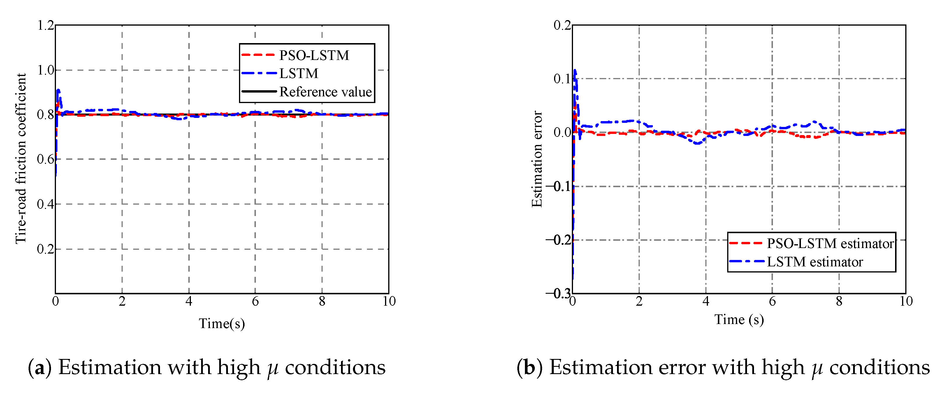
5.1.1. Analysis of Tire–Road Friction Coefficient Estimator

The performance of the tire–road friction coefficient estimator designed in Section 3 was verified under the condition of the given vehicle speed and the reference value of tire–road friction coefficient. The given speed of the experiment was 50 km/h, which was verified on roads with high tire–road friction coefficients (0.8), low tire–road friction coefficients (0.3), and split tire–road friction coefficients (0.9 to 0.4), respectively. The simulation results are shown in Figure 8, Figure 9 and Figure 10.

As can be seen in Figure 8 and Figure 9, the PSO-LSTM model can quickly converge to the reference value of tire–road friction coefficient on roads with high and low tire–road friction coefficients. In comparison, the LSTM model has a large overshoot in the initial stage of tire–road friction coefficient estimation and takes longer time to converge to the reference value of the tire–road friction coefficient. Between 4 s and 10 s, the LSTM model fluctuates significantly compared with the PSO-LSTM model. During the entire simulation process, the PSO-LSTM model has a slight overshoot in the estimated tire–road friction coefficient and the estimation error is within 0.12.

As shown in Figure 10, the PSO-LSTM model shows a more accurate estimation than the LSTM model in the simulation experiment with a split tire–road friction coefficient. When the simulation is carried out to 4.1 s, the reference value of tire–road friction coefficient changes abruptly from 0.9 to 0.4 and the estimation errors of both the PSO-LSTM model and the LSTM model peak at 4.1 s. The PSO-LSTM model converges rapidly at 4.14 s. In contrast, the LSTM model converges at 4.23 s and is characterized by a partial overshoot.

The RMSE of PSO-LSTM and LSTM are calculated according to Equation (20). As can be seen in

Table 3. The comparison of estimation error under different tire–road friction coefficients.

RMSE	PSO-LSTM	LSTM
Estimation with a high coefficient	0.0187	0.0245
Estimation with a low coefficient	0.0234	0.0297
Estimation with a split coefficient	0.0212	0.0269

, the estimation error of PSO-LSTM is smaller and has better stability on roads with different tire–road friction coefficients. In summary, the PSO-LSTM model and the LSTM model proposed in this paper can both achieve the accuracy standards for the estimation of the tire–road friction coefficient. However, in the simulation process, the PSO-LSTM model outperforms the LSTM model with less overshoot, quicker convergence, and a higher overall performance.

5.1.2. Analysis of Tire Cornering Stiffness for Different Tire–Road Friction Coefficients

To observe the influence of different tire–road friction coefficients on tire cornering stiffness, the absolute value of tire cornering stiffness was taken as the estimated result in this paper. The simulation results are shown in Figure 11. The simulations were validated on roads with high tire–road friction coefficients (0.9) and split tire–road friction coefficients (0.9 to 0.4), respectively. The figure illustrates how smoothly the tire cornering stiffness varies when a simulation is run on a road with a high tire–road friction coefficient and under the roads with split tire–road friction coefficients. However, the tire cornering stiffness fluctuates greatly when the tire–road friction coefficient varies to 0.4. The tire cornering stiffness decreases significantly.

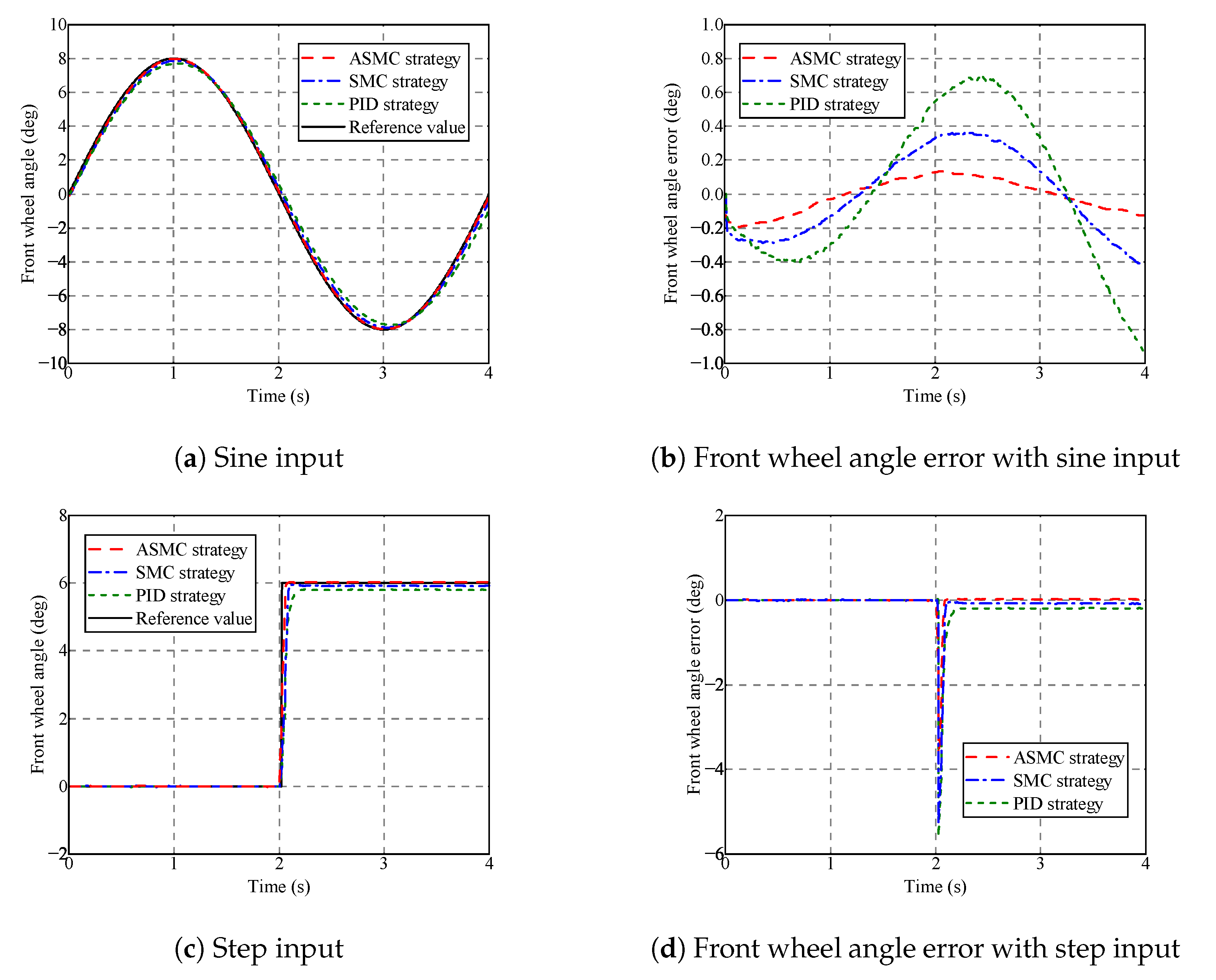
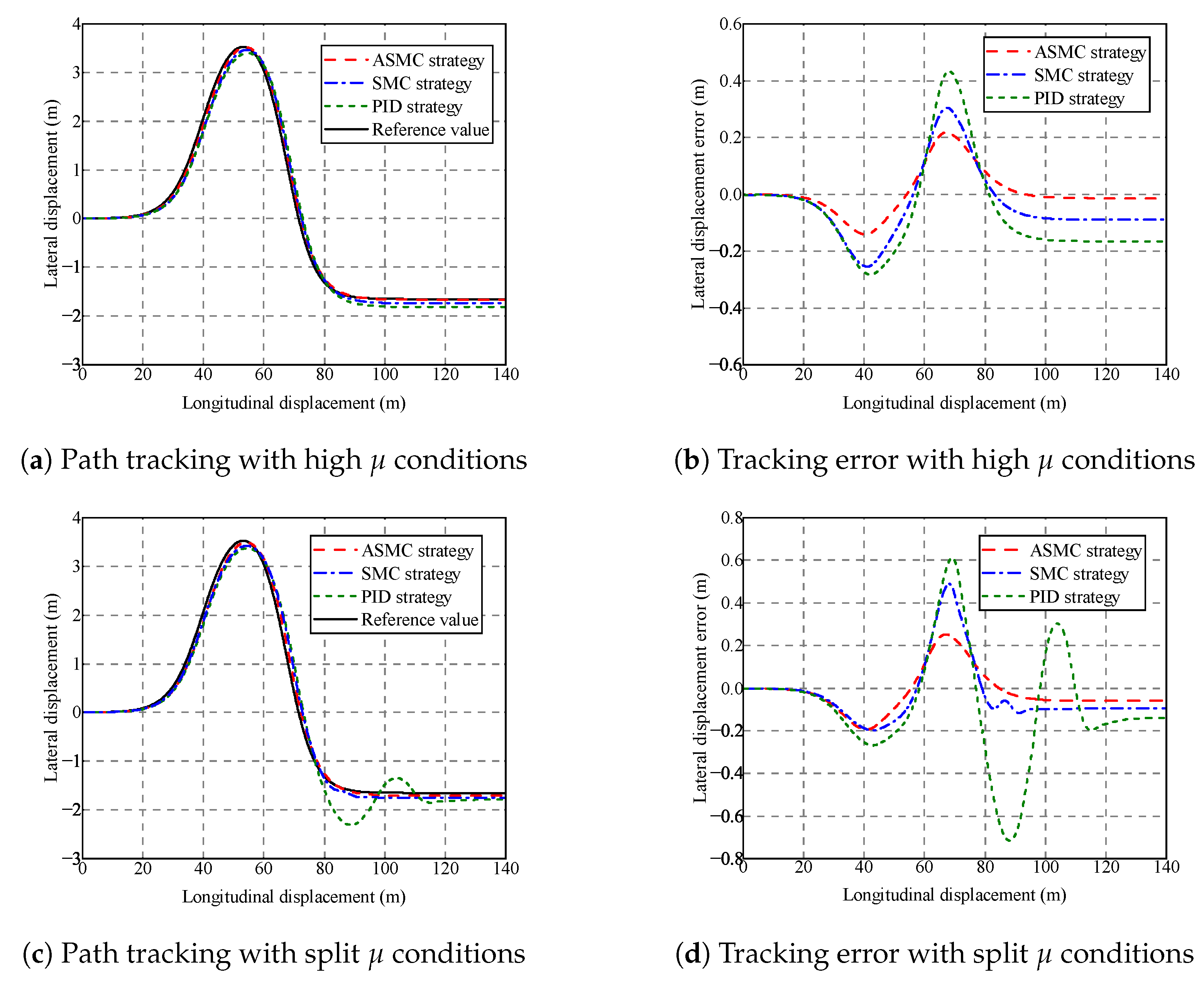
5.2. Validation of the Adaptive Sliding Mode Control Strategy

To verify the effectiveness of the adaptive sliding mode control strategy, which considers mechanical friction and the variation of tire cornering stiffness proposed in Section 4, the dynamic model of the dual-motor autonomous steering system was built by using CarSim and Simulink for simulation analysis. The PID control strategy and the sliding mode control strategy were chosen to compare with the proposed adaptive sliding mode control strategy in the same simulation environment to verify the performance of the proposed controller. The simulation results are shown in Figure 12 and Figure 13.

Figure 12a,c provide the results of the front wheel angle tracking accuracy for the proposed adaptive sliding mode control strategy, the SMC strategy and the PID strategy under sine and step input respectively. Figure 13a,c provide the results of path tracking performance under double lane change conditions on roads with high tire–road friction coefficients and split tire–road friction coefficients, respectively. Figure 12b,d provide the results of front wheel angle errors under sine input and step input, respectively. Figure 13b,d provide the tracking error results under double lane change conditions on roads with high tire–road friction coefficients and split tire–road friction coefficients respectively. The speed of the vehicle was set at 50 km/h.

As seen in Figure 12b, when the vehicle tracks at 50 km/h under sine input, the peak error of the front wheel angle for the adaptive sliding mode control strategy proposed in this paper is 0.132, while the peak errors of the front wheel angle for the SMC strategy and the PID strategy are 0.364 and 0.685. Compared with the two control strategies, a significant reduction of 63.7% and 80.7% is achieved with the proposed ASMC strategy correspondingly. As seen in Figure 12d, the peak error of the front wheel angle for the proposed adaptive sliding mode control strategy under step input is 3.77, while the peak errors of the front wheel angle for the SMC strategy and the PID strategy are 5.3 and 5.58. Compared with the two control strategies, a significant reduction of 28.8% and 32.4% is achieved with the proposed ASMC strategy correspondingly. It can be seen from the figures that the proposed ASMC control strategy improves the accuracy of angle tracking.

Furthermore, when the target front wheel angle suddenly changes, the adaptive sliding mode control strategy reacts quickly and has better tracking performance. As seen in Figure 13b, the peak lateral displacement errors for the adaptive sliding mode control strategy proposed in this paper is 0.2, while the peak error of lateral displacement for the SMC strategy and the PID strategy are 0.295 and 0.374. Compared with the two control strategies, a significant reduction of 32.2% and 46.5% is realized. As seen in Figure 13d, the peak lateral displacement error for the adaptive sliding mode control strategy under split $\mu$ condition is 0.25, while the peak error of lateral displacement for the SMC strategy and the PID strategy are 0.466 and 0.59. Compared with the two control strategies, a significant reduction of 46.3% and 57.6% is realized. When the tire–road friction coefficient changes abruptly to a low tire–road friction coefficient of 0.4, the adaptive sliding mode control strategy performs better stability. This is because the adaptive reaching law proposed in this paper adaptively adjusts the reaching law parameters according to the system state to obtain a better control response. The sliding surface with an integral error in the ASMC strategy can reduce the effect of steady state error when the nonlinear disturbance exists. Henceforth, the proposed adaptive sliding mode control strategy considering mechanical friction and the variation of tire cornering stiffness efficiently improves the tracking accuracy and provides superior stability.

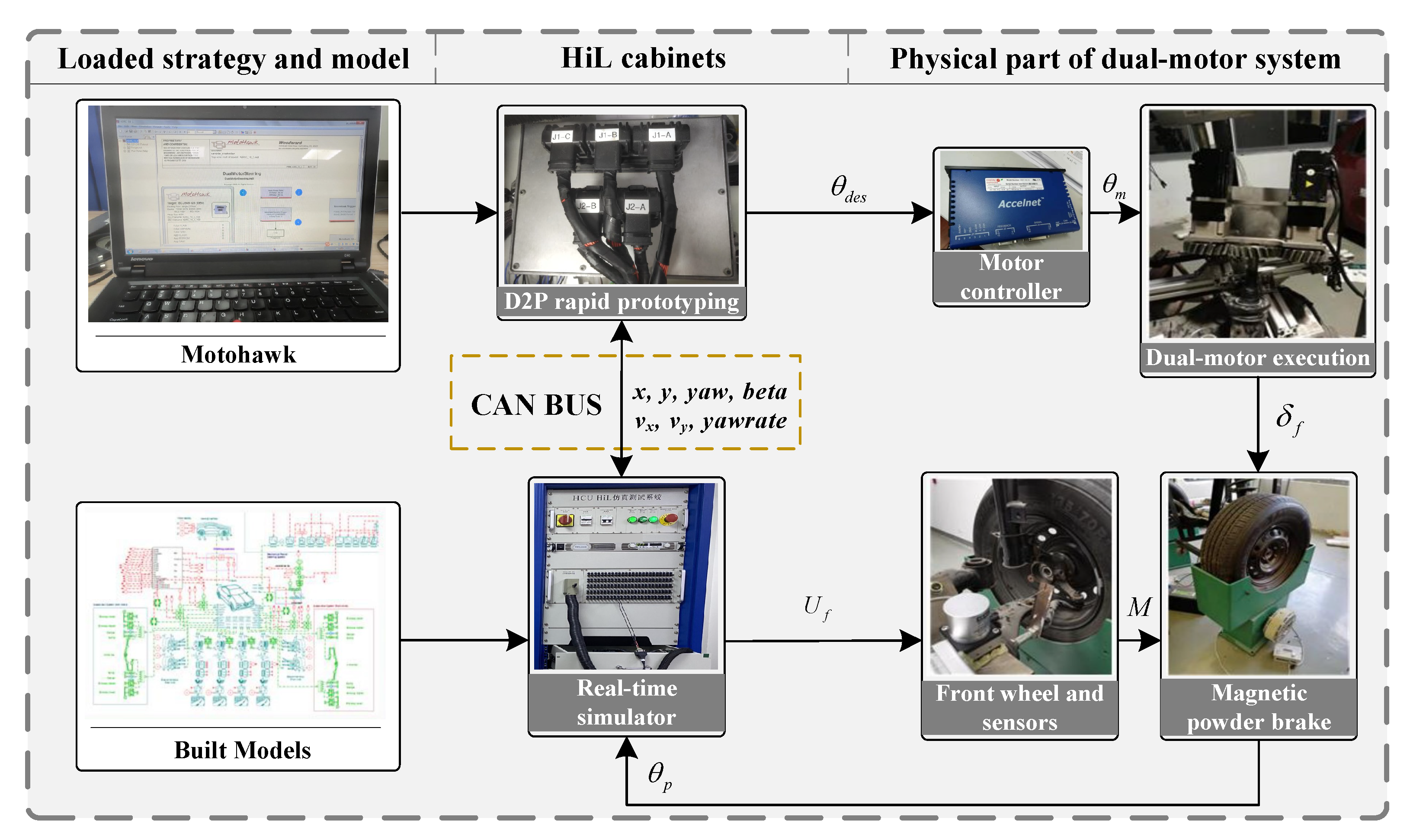
6. Hardware-in-Loop Test Results

To further verify the effectiveness of the control strategy of the dual-motor autonomous steering system proposed in this paper, an HiL experimental station is built, which consists of an NI real-time simulator, a D2P controller, a host computer and a dual-motor autonomous steering system test platform. The flow chart of the structure is shown in Figure 14.

The experiment was conducted as follows: Firstly, the vehicle model was loaded into the NI real-time simulator via Veristand and the control strategy was compiled with MotoHawk. Secondly, the control strategy was loaded into the D2P controller, and the CAN communication module was configured to communicate with the D2P, front wheel angle sensor and magnetic powder brake via the Veristand software. Finally, the front wheel angle sensor transmitted the measured front wheel angle to the NI real-time simulator, which sent control voltage to the magnetic powder brake and output vehicle status information to the D2P controller, which further transmitted the target angle to the steering motor controller via CAN communication and drove the steering motors to track the target angle.

Roads with high tire–road friction coefficients (0.8) and roads with split tire–road friction coefficients (0.9 to 0.4) were set up. Path tracking control under the double lane change condition was performed at a vehicle speed of 50 km/h. As seen in Figure 15b, the peak lateral displacement errors for the adaptive sliding mode control strategy proposed in this paper were 0.217, while the peak error of lateral displacement for the SMC strategy and the PID strategy were 0.303 and 0.433. Compared with the two control strategies, a significant reduction of 28.3% and 49.8% was realized correspondingly. As seen in Figure 15d, the peak lateral displacement error for the adaptive sliding mode control strategy under split $\mu$ condition was 0.262, while the peak error of lateral displacement for the SMC strategy and the PID strategy were 0.476 and 0.606. Compared with the two control strategies, a significant reduction of 44.9% and 56.7% was realized correspondingly. It can be seen that in the HiL experiments that compared the SMC control strategy with the PID control strategy, the ASMC control strategy proposed in this paper had a significantly better performance of path tracking and still had good path tracking accuracy when the tire–road friction coefficients changes abruptly to 0.4. This is due to the fact that the ASMC control strategy, which considers mechanical friction and the variation of tire cornering stiffness proposed in this paper, has strong anti-disturbance ability to nonlinear characteristics, affecting the path tracking control of the lower actuator. In summary, the HiL tests verify the control strategy of the dual-motor autonomous steering system considering mechanical friction and the variation of tire cornering stiffness outperforms the SMC control strategy and the PID control strategy in terms of path tracking performance.

7. Conclusions

This paper presents a path tracking control strategy for a dual-motor autonomous steering system for intelligent vehicles, considering nonlinear characteristics to reduce path tracking error due to friction in the mechanical mechanism, nonlinearity in tires, the uncertainties in the transmission parameters and road conditions. First, the LuGre friction model was applied to the dual-motor autonomous steering system for friction compensation, and the model for self-aligning torque was established. Second, a PSO-LSTM neural network-based estimator was designed to estimate the tire–road friction coefficient. The tire cornering stiffness under different tire–road friction coefficients was estimated through the recursive least-square algorithm. Based on the estimated stiffness, an adaptive sliding mode control strategy based on field-oriented control and an LQR path tracking controller were designed. Finally, the method described in this paper was validated by simulation and HiL tests. The results show that the control strategy proposed in this paper can significantly improve path tracking performance. In future tasks, the strategy of vehicle stability control will be further investigated and combined with the control strategy of the dual-motor autonomous steering system. Through the design and calibration of steering motors, the control strategy will be further applied to real vehicle tests to improve the stability under multi-nonlinear conditions while ensuring path tracking performance.

References

1. Chen, T.; Chen, L.; Xu, X.; Cai, Y.; Jiang, H.; Sun, X. Passive fault-tolerant path following control of autonomous distributed drive electric vehicle considering steering system fault. Mech. Syst. Signal Process. 2019, 123, 298–315. [Google Scholar] [CrossRef]
2. Xie, J.; Xu, X.; Wang, F.; Liu, Z.; Chen, L. Coordination Control Strategy for Human-Machine Cooperative Steering of Intelligent Vehicles: A Reinforcement Learning Approach. IEEE Trans. Intell. Transp. Syst. 2022, 23, 21163–21177. [Google Scholar] [CrossRef]
3. Yan, M.; Chen, W.; Wang, Q.; Zhao, Q.; Liang, X.; Cai, B. Human–Machine Cooperative Control of Intelligent Vehicles for Lane Keeping—Considering Safety of the Intended Functionality. Actuators 2021, 10, 210. [Google Scholar] [CrossRef]
4. Lin, F.; Sun, M.; Wu, J.; Qian, C. Path Tracking Control of Autonomous Vehicle Based on Nonlinear Tire Model. Actuators 2021, 10, 242. [Google Scholar] [CrossRef]
5. Yang, T.; Bai, Z.; Li, Z.; Feng, N.; Chen, L. Intelligent Vehicle Lateral Control Method Based on Feedforward + Predictive LQR Algorithm. Actuators 2021, 10, 228. [Google Scholar] [CrossRef]
6. Zou, S.; Zhao, W. Synchronization and stability control of dual-motor intelligent steer-by-wire vehicle. Mech. Syst. Signal Process. 2020, 145, 106925. [Google Scholar] [CrossRef]
7. Xu, X.; Su, P.; Wang, F.; Chen, L.; Xie, J. Coordinated control of dual-motor using the interval type-2 fuzzy logic in autonomous steering system of AGV. Int. J. Fuzzy Syst. 2021, 23, 1070–1086. [Google Scholar] [CrossRef]
8. He, L.; Chen, G.; Zheng, H. Fault tolerant control method of dual steering actuator motors for steer-by-wire system. Int. J. Automot. Technol. 2015, 16, 977–987. [Google Scholar] [CrossRef]
9. Mi, J.; Wang, T.; Lian, X. A system-level dual-redundancy steer-by-wire system. Proc. Inst. Mech. Eng. Part D J. Automob. Eng. 2021, 235, 3002–3025. [Google Scholar] [CrossRef]
10. Anwar, S.; Niu, W. A Nonlinear Observer Based Analytical Redundancy for Predictive Fault Tolerant Control of a Steer-by-Wire System. Asian J. Control 2014, 16, 321–334. [Google Scholar] [CrossRef]
11. Xie, J.; Xu, X.; Wang, F.; Tang, Z.; Chen, L. Adaptive coordination control strategy for path-following of DDAEV with neural network based moving weight coefficients. Trans. Inst. Meas. Control 2022, in press. [CrossRef]
12. Huang, C.; Huang, H.; Naghdy, F. Actuator fault tolerant control for steer-by-wire systems. Int. J. Control 2021, 94, 3123–3134. [Google Scholar] [CrossRef]
13. Li, S.; Wang, G.; Chen, G.; Chen, H.; Zhang, B. Tire state stiffness prediction for improving path tracking control during emergency collision avoidance. IEEE Access 2019, 7, 179658–179669. [Google Scholar] [CrossRef]
14. Peng, H.; Wang, W.; An, Q.; Xiang, C.; Li, L. Path tracking and direct yaw moment coordinated control based on robust MPC with the finite time horizon for autonomous independent-drive vehicles. IEEE Trans. Veh. Technol. 2020, 69, 6053–6066. [Google Scholar] [CrossRef]
15. Hao, J.; Liang, C.; Yang, R.; Lin, Z. A recognition method of road adhesion coefficient based on Recurrent Neural Network. In Proceedings of the 2021 International Conference on Computer Information Science and Artificial Intelligence (CISAI), Kunming, China, 17–19 September 2021; pp. 79–82. [Google Scholar]
16. Yu, M.; Xu, X.; Wu, C.; Li, S.; Li, M.; Chen, H. Research on the prediction model of the friction coefficient of asphalt pavement based on tire-pavement coupling. Adv. Mater. Sci. Eng. 2021, 2021, 6650525. [Google Scholar] [CrossRef]
17. Ribeiro, A.M.; Moutinho, A.; Fioravanti, A.R.; Paiva, E.C. Estimation of tire–road friction for road vehicles: A time delay neural network approach. J. Braz. Soc. Mech. Sci. Eng. 2020, 42, 1–12. [Google Scholar] [CrossRef] [Green Version]
18. Sun, Z.; Zheng, J.; Wang, H.; Man, Z. Adaptive fast non-singular terminal sliding mode control for a vehicle steer-by-wire system. IET Control Theory Appl. 2017, 11, 1245–1254. [Google Scholar] [CrossRef]
19. Kazemi, R.; Janbakhsh, A.A. Nonlinear adaptive sliding mode control for vehicle handling improvement via steer-by-wire. Int. J. Automot. Technol. 2010, 11, 345–354. [Google Scholar] [CrossRef]
20. Li, H.; Zhang, T.; Tie, M.; Wang, Y. Fuzzy-Based Adaptive Higher-Order Sliding Mode Control for Uncertain Steer-by-Wire System. J. Dyn. Syst. Meas. Control 2022, 144, 041005. [Google Scholar] [CrossRef]
21. Wang, Z. Adaptive fuzzy system compensation based Model-free control for steer-by-wire systems with uncertainty. Int. J. Innov. Comput. Inf. Control 2021, 17, 141–152. [Google Scholar]
22. Pikunov, D.; Stefanski, A. Numerical analysis of the friction-induced oscillator of Duffing’s type with modified LuGre friction model. J. Sound Vib. 2019, 440, 23–33. [Google Scholar] [CrossRef]
23. Shi, Q.; Zhang, H. Fault diagnosis of an autonomous vehicle with an improved SVM algorithm subject to unbalanced data sets. IEEE Trans. Ind. Electron. 2020, 68, 6248–6256. [Google Scholar] [CrossRef]
24. Yu, Y.; Si, X.; Hu, C.; Zhang, J. A review of recurrent neural networks: LSTM cells and network architectures. Neural Comput. 2019, 31, 1235–1270. [Google Scholar] [CrossRef]
25. Smagulova, K.; James, A.P. A survey on LSTM memristive neural network architectures and applications. Eur. Phys. J. Spec. Top. 2019, 228, 2313–2324. [Google Scholar] [CrossRef]
26. Karim, F.; Majumdar, S.; Darabi, H.; Chen, S. LSTM fully convolutional networks for time series classification. IEEE Access 2017, 6, 1662–1669. [Google Scholar] [CrossRef]
27. Yang, J.; He, L.; Fu, S. An improved PSO-based charging strategy of electric vehicles in electrical distribution grid. Appl. Energy 2014, 128, 82–92. [Google Scholar] [CrossRef]
28. Ding, Y.; Zhang, W.; Yu, L.; Lu, K. The accuracy and efficiency of GA and PSO optimization schemes on estimating reaction kinetic parameters of biomass pyrolysis. Energy 2019, 176, 582–588. [Google Scholar] [CrossRef]
29. Chu, Z.; Chen, N.; Zhang, N.; Li, G. Path-tracking for autonomous vehicles with on-line estimation of axle cornering stiffnesses. In Proceedings of the 2019 Chinese Control Conference (CCC), Guangzhou, China, 27–30 July 2019; pp. 6651–6657. [Google Scholar]
30. Jiang, C.; Wang, Q.; Li, Z.; Zhang, N.; Ding, H. Nonsingular terminal sliding mode control of PMSM based on improved exponential reaching law. Electronics 2021, 10, 1776. [Google Scholar] [CrossRef]
Figure 1. The dual-motor autonomous steering system model.
Actuators 12 00097 g001
Figure 2. Tire slip characteristic curve.
Actuators 12 00097 g002
Figure 3. The LSTM structure.
Actuators 12 00097 g003
Figure 4. The flow chart of tire–road friction estimation based on the PSO-LSTM.
Actuators 12 00097 g004
Figure 5. Dual-motor autonomous steering system control strategy.
Actuators 12 00097 g005
Figure 6. Model of the vehicle tracking error.
Actuators 12 00097 g006
Figure 7. The overall control scheme.
Actuators 12 00097 g007
Figure 8. Simulation results with high tire–road friction coefficients.
Actuators 12 00097 g008
Figure 9. Simulation results with low tire–road friction coefficients.
Actuators 12 00097 g009
Figure 10. Simulation results with split tire–road friction coefficients.
Actuators 12 00097 g010
Figure 11. Tire cornering stiffness.
Actuators 12 00097 g011
Figure 12. Simulation results of front wheel angle.
Actuators 12 00097 g012
Figure 13. Simulation results of path tracking.
Actuators 12 00097 g013
Figure 14. HiL test platform.
Actuators 12 00097 g014
Figure 15. Experimental results of path tracking.
Actuators 12 00097 g015