1. Introduction
The interference of support mechanisms in transonic wind tunnels is serious. In the transonic range, the flow is more complex [
1]. There are both subsonic and supersonic regions in the flow field, and the aerodynamic force and torque change dramatically with the change in Mach number [
2].
When space shuttles, spacecraft, and aircraft fly at a high angle of attack, it is easy to produce airflow separation, rupture, and longitudinal and transverse aerodynamic coupling [
3], resulting in runaway accidents [
4,
5]. Additionally, intercontinental missiles, human-crewed spacecraft, and other vehicles are prone to dynamic instability in the process of rotary reentry [
6]. The dynamic derivative of the vehicle is the key parameter to studying such problems. The dynamic derivative wind tunnel test uses forced or free oscillation equipment to simulate the rigid motion mode of the vehicle to obtain the dynamic stability derivative [
7]. For the dynamic derivative experiment, no matter what angle of the balance support mechanism [
8] is used, the flow structure at the bottom of the model will be damaged, and there will inevitably be some interference, resulting in low repeatability and accuracy of the experiment. Because of this, the wind tunnel test technology for vehicle models without the interference of support mechanisms is still being explored and developed. The MSBS uses suspension control technology [
9,
10] to realize the non-contact suspension of the vehicle model and the non-contact measurement of aerodynamic parameters, which is the development direction of wind tunnels in the future [
11].
MIT, NASA, and Old Dominion University have further studied the MSBS and conducted aerodynamic tests on the spacecraft atmospheric reentry module with the MSBS [
12]. There is an iron core ball inside the model. The inductive position sensor is used to detect the position of the suspension model. During suspension control, the inductive sensor is not affected by the ambient light intensity and has less signal noise. However, this method cannot detect the model’s rotation, so the rotation direction can not be controlled [
13,
14].
The suspension model realizes the non-contact suspension through the interaction between the electromagnet and the permanent magnet. The electromagnetic force supporting the model in the MSBS is a non-contact force. Compared with the maglev train [
15,
16] and maglev bearing [
17], the suspension gap is large, and the magnetic effect makes it challenging to achieve the best state. The x-direction bearing capacity of the model in a supersonic wind tunnel [
18,
19] is much larger than that in a low-speed wind tunnel. The large gap suspension system is challenging to model. The existing literature needs to establish a complex relationship between the position current and the electromagnetic force, and there is no existing state equation for the MSBS. In addition to using PID control, other model-based control algorithms are difficult to apply [
11].
When the wind tunnel is activated, a rapid shock load appears. Some researchers take the levitation ball as the object and propose an adaptive time repair adaptive control algorithm to improve the anti-interference ability and stability of the levitation ball. In recent years, many scholars have conducted in-depth research on the ARDC (active disturbance rejection control) technique, applied it to many fields, achieved certain results, and promoted the development of the ARDC field [
20,
21,
22,
23]. Few scholars have studied the anti-interference control of the MSBS. In this paper, the equation of the state of the magnetic suspension control system is established for these problems, and an anti-interference framework suitable for the MSBS is given to resist the interference of external forces.
The aerodynamic force of the suspension model in the wind tunnel changes, which will affect the position control accuracy of the suspension model and reduce the test capacity of the MSBS. There is little research on the suppression strategy of aerodynamic interference of the MSBS. To study this accurately, it is necessary to model the electromagnetic field and force. However, the magnetic field of maglev balance is complex, and many factors, such as coil space relative position, shape, and magnetic rod, affect the magnetic field and electromagnetic force. Most of the factors have a nonlinear effect on the magnetic field. Then, estimating the accurate external interference quickly or in real time is also tricky. To solve urgent problems, this paper theoretically calculates and deduces the state equation of MSBS and provides a disturbance force compensation framework for magnetic suspension balance system.
The main contributions of this article are as follows. (1) For the problem of the difficulty of modeling nonlinear magnetic fields in MSBS, the mathematical expression of the electromagnetic field and electromagnetic force of the MSBS along the airflow direction is derived. (2) A fast disturbance estimation algorithm combining a tracking differentiator and observer is proposed, which can accurately obtain the external disturbance force in real-time and quickly. (3) A disturbance force compensation framework is proposed, which can effectively reduce the influence of external interference on the control system and improve the accuracy of the control system.
This article is organized as follows:
In
Section 2, the MSBS is analyzed and modeled to analyze its electromagnetic field and force characteristics. The state equation of the open-loop system is established. In
Section 3, the influence of external disturbance force on the nominal controller is analyzed. In
Section 4, the tracking differentiator is used to obtain the speed and acceleration of the suspension model. Then the coil’s current and the suspended object’s position can be directly obtained by the sensor, which is used to calculate and estimate the external interference.
Section 5 inputs the estimated external disturbance force to the original controller to form a disturbance force compensation framework. The anti-interference ability of the disturbance force compensation framework is simulated and analyzed. In
Section 6, the proposed control algorithm is experimentally tested and verified.
2. Establishment of Physical Model
The electromagnetic coil distribution structure of the MSBS is shown in
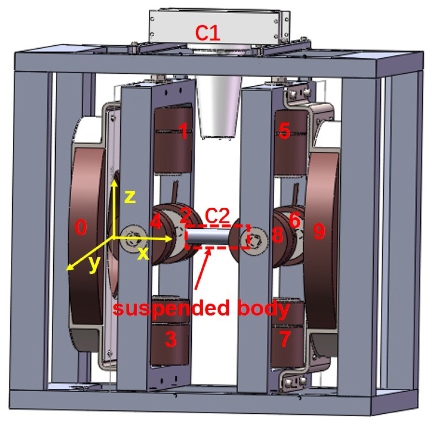
Figure 1. The electromagnetic coils of the MSBS are divided into five pairs, one in the x-direction, two distributed in the y-direction, and two pairs distributed in the z-direction. The head and tail of the suspension model are not only distributed with a pair of x-direction coils but also a pair of y-direction coils. The suspension model contains a permanent magnet. The repulsion of one coil adjusts the displacement in each direction to the suspension model and the suction of the other coil to the suspension model. Coils 0 and 9 are x-direction coils, which are used to control the x-direction movement of the suspension model. Coils 1, 3, 5, and 7 are z-direction coils used to control up, down, and pitch movements. Coils 2, 4, 6, and 8 are y-direction and are used to control the movement in the left, right, and yaw directions. At the same time, the rotating magnetic field is superimposed by coils 5, 6, 7, and 8 and is used to control the movement in the rolling direction. C1 is a visual sensor used to measure the position of the suspended model. C2 is the position of the suspended model.
The airflow direction is consistent with the x-direction, and the interference of the airflow is also mainly along the x-direction, so this article mainly focuses on the control system in the x-direction.
The schematic diagram of the x-direction coil and suspension model is shown in
Figure 2. Then, the physical equation of the MSBS in the x-direction with the rod aligned with the coil axis is deduced. The magnetization curve, shape, and size of the permanent magnet model material are known, and the coil size, position relationship, and number of turns are known. These known quantities are used to calculate and analyze the x-direction electromagnetic field and the electromagnetic force on the magnetic rod that is the suspension model.
The simplified formula of x-direction electromagnetic force is [
24]
where
is the generalized magnetic moment of the magnetic rod,
is the magnetic field intensity of the x-direction coil, and
x is the x-direction position coordinate.
where
is the length of the magnetic rod which is 0.096 m,
is the radius of the magnetic rod, which is 0.005 m, and
is the remanence of the magnetic rod, which is 0.6 T. The calculated
is
Wbm.
The magnetic flux density generated by the electromagnetic coil in the x-direction direction is
where
I is the current passing through the electromagnet coil,
is the radius of the coil,
N is the number of coil turns, and
is the x-direction unit vector.
Because it is a hollow coil, the relative permeability is approximately equal to
, which is the vacuum permeability. Therefore, the relationship between magnetic field intensity and magnetic flux density is as follows
The magnetic field intensity generated by the x-direction coil is
where
is the equivalent radius of the x-direction air core coil which is 0.2 m,
I is the current, and
N is the number of turns, which is 250.
Equation (
6) can be deduced by taking the derivative of
in Equation (
5).
The electromagnetic force on the magnetic rod is decomposed into countless small parts. The expression of the electromagnetic force of each fraction is as follows:
The total electromagnetic force is obtained by integrating the electromagnetic force on the magnetic rod along the x-direction.
Equation (
9) is obtained by calculating Equation (
8), which is the expression of the total electromagnetic force.
The relationship between the magnetic force and the position of the magnetic rod is shown in
Figure 3, where x is the center of mass position of the magnetic rod. The current of the coil is 50 A. The green curve is the force generated by coil 0 on the magnetic rod. The red curve is the force generated by coil 9 on the magnetic rod. The blue curve is the total electromagnetic force on the magnetic rod. It can be concluded that the electromagnetic force changes nonlinearly with the position.
The relationship between voltage and current applied to both ends of the electromagnet is expressed as follows:
where
u is the voltage applied to both ends of the actuator coil,
L is the inductance of the coil, and
R is the resistance of the coil. The dynamic equation of the suspension model is as follows:
where
is the mass of the suspension, which is 71 g,
is the x-direction electromagnetic force, and
is the aerodynamic resistance.
Let
. The state model of the MSBS without considering the interference is as follows,
where
is the system output, that is, the x-direction position of the center of mass of the magnetic rod.
Let
The function matrix is as follows:
The simplified state equation of the MSBS is as follows:
3. Double-Loop Feedback Controller and Influence of External Force Interference
Without feedback control, the MSBS belongs to an unstable system and the position of the suspension model will diverge. Because the current phase of the coil seriously lags behind the voltage at both ends, it is not easy to control the system if the current feedback control is not carried out to improve the responsiveness of the coil. In this paper, the position and current double-loop feedback control is adopted, and the current loop is used to improve the coil’s response-ability and reduce the system’s order. The position feedback control is used to adjust the position of the suspension model in real time. The control law of a double-loop feedback controller is as follows:
where
is the proportional feedback coefficient,
is the differential feedback coefficient,
is the integral feedback coefficient,
is the circuit loop feedback coefficient, and
r is the target value of the controller.
is acquired by the current sensor.
We replace
u in Equation (
14) with a double-loop feedback controller
The simplified expression of the state model with double-loop feedback control is as follows:
The stress and environment of the same suspension model will change significantly at different flow velocities. When the flow velocity is low, the pressure and density change little, and the flow field is stable. The model will produce shock waves in the supersonic flow field. When the air flows through the shock wavefront, the parameters such as pressure, density, and velocity will change abruptly, which is no longer a continuous function of space. At this time, the model’s aerodynamic load force and fluctuation value will become larger, leading to the suspension model’s coupling vibration on aerodynamic and electromagnetic forces. This sudden change and discontinuous external force interference will lead to extreme control system instability. The x-direction position will deviate from the target position seriously and not be able to meet the accuracy requirements of the wind tunnel test.
In the case of interference, the expression of the x-direction state equation of the suspension system with double-loop feedback control is as follows:
where
is the external interference, which can be wind force or other forces.
.
We apply a square wave interference with a period of 2 s and amplitude of 0.3 N to the system. When there is interference and no interference, the control effect of x-direction displacement is compared, as shown in
Figure 4. The solid blue curve is the x-direction position of the suspended model under the action of no external interference. It can be seen that it quickly approaches the target position of 0.12 m from the initial position, which is 0.125 m, and then remains stable. However, the red dotted curve is the coordinate of the suspended material center under the action of interference. It can be seen that under the action of interference, the position of suspension control is constantly changing and fluctuating, the x-direction position is changing between 0.098 and 0.12 m, and the fluctuation value is 0.012 m.
4. Real-Time External Disturbing Force Estimation
When there is an external force disturbance, the acceleration of the suspended object consists of two parts, the external force disturbance generates one and the electromagnetic force of the x-direction coil generates the other. Therefore, the acceleration generated by the external force disturbance can be obtained by subtracting the acceleration generated by the electromagnetic force of the x-direction coil from the total acceleration. Therefore, the acceleration of the suspension model needs to be obtained first. The x-direction position of the suspension model can be measured directly by a CCD sensor [
25]. Theoretically, acceleration can be obtained by differentiating the position twice. However, the differential operation is susceptible to noise, which will amplify the signal’s noise and reduce the signal-to-noise ratio. In this paper, the tracking differentiator is introduced to obtain the signal’s differential signal, significantly reduce the influence of noise, and improve the signal-to-noise ratio. The constructed tracking differentiator [
26,
27] is as follows:
where
is the sensor measurement signal, which is the input of the tracking differentiator,
is the tracking estimation of the input signal, and
is the estimation of the differential of the input signal.
h is the calculation step and
is the function. The expression of
is as follows [
28]:
where
is the speed factor, and the performance of the tracking differentiator can be adjusted by changing the size of the modified parameter.
and
are intermediate variables. After the velocity of the suspended object is obtained by the tracking differentiator, it is differentiated by the differentiator, and then the estimated acceleration is obtained after filtering.
The stability is proved as follows:
Adjusting
can make the following formula hold.
and
are less than infinity.
The following expression is also satisfied
Let the estimation error of
be
. Let the estimation error of
be
. After converting a discrete system into a continuous system, the system can be extended to the following expression.
The extended error system matrix
is
The extended error system matrix
is
The expression of error is
The characteristic equation is
When the following expression is satisfied, the characteristic root of the characteristic matrix of the system is on the left of the s plane.
When the time approaches infinity, the error expression is as follows
Because is bounded and the error is bounded, the estimation framework is stable.
As shown in Equation (
21), there is a high-order error
between the estimated acceleration and the acceleration of the suspension model.
where
is the acceleration of the real system and
is the estimated acceleration.
For disturbance acquisition, although the electromagnetic force generated by the coil on the suspension cannot be obtained directly, the electromagnetic force can be calculated and estimated by the current of the coil and the position state of the suspension model.
The estimated x-direction electromagnetic force is as follows:
where
is the current signal obtained by the current sensor, and
is the x-direction position signal obtained by the CCD position sensor.
is a high-order error between the estimated electromagnetic force and the electromagnetic force of the suspension model.
is the estimated disturbing force, which is as follows:
The comparison diagram between the observed external interference and the real applied interference is shown in
Figure 5. The solid red line in
Figure 5 represents the real external interference applied on the suspended object, which is a square wave interference with a period of 2 s and an amplitude of 0.3 N. The blue dotted line is the observed interference, and the estimated interference is consistent with the actual interference. However, there is an overshoot oscillation at the rising and falling edges of the change of interference, and there is a small amplitude oscillation in the middle.
5. Disturbance Force Compensation Framework for MSBS
In the previous section, the disturbance was obtained. Theoretically, the influence of external force interference on the control system can be compensated by applying a force with the same amplitude and opposite direction to the suspension model. However, in practice, only voltage can be applied to the coil to generate current, which exerts a force on the suspension model to weaken the external interference. Due to the influence of the actuator and sensor delay and error, the estimated external interference needs to be multiplied by a constant coefficient and feedback to the original control system. The interference feedback coefficient is adjusted to minimize the influence of the disturbance force on the MSBS. The control law of the disturbance force compensation framework (DFCF) is as follows:
The state equation expression of the x-direction control system is simplified as follows:
The structure of the control strategy of the DFCF is shown in
Figure 6. The dotted line box represents the disturbance force compensation controller. The input on the controller’s left is the target position to be controlled, and the output is the control voltage to the coil, which contains two parts. The light red solid line box represents the double-loop controller of the x-direction position current of the MSBS, and the light red dotted line is the disturbance estimator. The input of the disturbance estimator is the position of the suspended model, which is input to the tracking differentiator to obtain the velocity. After the velocity is differentiated again, it is filtered to obtain the acceleration and then multiplied by the mass of the suspended object to obtain the total force on the suspended model. The estimated interference is obtained by subtracting the estimated electromagnetic force from the total force, and the estimated interference is multiplied by the coefficient
. It is subtracted from the double-loop controller as the output of the new controller, which contains the disturbance compensation term. The solid blue wireframe represents the actual x-direction physical model of the MSBS, the controlled object, which includes two parts: the suspended model and the x-direction coil. The input of the suspended model is the electromagnetic force and external interference. The input of the x-direction coil is the control voltage, and the output is the x-direction electromagnetic force to the suspension. Some researchers have proved the stability of PID in theory [
29]. This control framework is improved on the basis of PID control, and we need to adjust the controller parameters to make the system stable. The following is verified by simulation and experiment.
Figure 7 shows the control effect of the DFCF strategy. The blue curve shows the position of the suspension model without external interference. It can be seen that it quickly approaches the target position from the initial position and then remains stable. However, the red curve is the position of the suspension model under the action of interference. It can be seen that under the action of interference, the position of the suspension model is constantly changing and fluctuating, the x-direction position is changing between 0.098 and 0.12 m, and the fluctuation value is 0.022 m. The green curve is the displacement control curve of the DFCF. It can be seen that although the displacement will fluctuate under the interference of external force, the fluctuation amplitude is smaller than the red curve, only half of the red curve. The x-direction position changes between 0.11 and 0.12 m and the fluctuation amplitude is 0.01 m.
Theoretically, increasing the disturbance feedback coefficient
can improve the anti-external disturbance performance of the controller, but when
exceeds a certain value, the system will have divergent instability. In order to explore the reason, different disturbance feedback coefficients
are set, and then the disturbance tracking effect is compared. As shown in
Figure 8, the green curve is the estimated external disturbance when
is zero. The red curve is a
of 90, the rising and falling edges of the estimated change of external disturbance force have slight jitter, and there is no oscillation when there is no change of external disturbance force. The yellow curve is a
of 105, the rising and falling edges of the change of external disturbance force shake violently, and there is also a large amplitude oscillation when the external disturbance force does not change. The blue curve is a curve where
is 100, and its effect is between the red curve and the yellow curve. Therefore, the feedback coefficient should be manageable. If it is too large, the fluctuation of the disturbance observed while the controller is adjusting will be large, making the system divergent and unstable.
The wind force in the x-direction is sometimes a random disturbance.
Figure 9 shows the control effect of the DFCF on random external disturbance. The blue curve is the position of the suspension model without external interference. It can be seen that it quickly approaches the target position from the initial position and then remains stable. However, the red curve is the position of the suspension model under the action of random external disturbance. It can be seen that under the action of the random interference, the position of the suspension model control constantly fluctuates, the x-direction position changes between 0.117 and 0.124 m, and the fluctuation value is 0.007 m. The green curve is the displacement control curve of the DFCF. It can be seen that although the displacement will fluctuate under the random external interference, the fluctuation amplitude is smaller than the red curve, only half of the red curve. The x-direction position changes between 0.118 and 0.122 m, and the fluctuation amplitude is 0.004 m. The amplitude of the random interference is 0.4 N.
7. Conclusions and Future Work
In this paper, taking the x-direction target position of the suspension model in the MSBS as the control object, the expressions of the electromagnetic field, the electromagnetic force, and the system state equation are derived. It is found that the MSBS is nonlinear, and the x-direction electromagnetic force on the suspension model is a multivariate nonlinear function of position and current. According to the derived physical equation expression, a digital simulation platform was built.
Then, a real-time disturbance force compensation framework for the MSBS was proposed. Under this framework, smoother suspension acceleration is obtained by the method based on a tracking differentiator, and the total force of the suspension is obtained by multiplying the acceleration by the mass. The electromagnetic force of the control output is directly estimated by the current and position, and the disturbance is obtained by subtracting the estimated electromagnetic force of the control output from the total force. In the digital simulation platform, the pulsation and random interference of aerodynamic force are simulated, and it is shown that the DFCF has more anti-interference ability than the traditional MSBS control algorithm. The simulated square wave and random interference are more rigorous than aerodynamic interference.
Finally, the impact force of the weight is applied to the controlled object to verify that the algorithm proposed in this paper can effectively suppress the external interference of MSBS in the experiment. Future research focuses on (1) exploring how to give the algorithm further anti-interference resistance, such as increasing it by more than 50%; (2) testing the algorithm’s ability to resist aerodynamic interference in an actual wind tunnel flow field.


