Abstract
After a short overview of the COLIBRI project, this paper considers the cycle-averaged flight dynamics of a flapping-wing robot near hovering, taking advantage of the weak coupling between the roll and pitch axes. The system is naturally unstable; it needs to be stabilized actively, which requires an attitude reconstruction. Due to the flapping of the wings, the system is subject to a strong periodic noise at the flapping frequency and its higher harmonics; the resulting axial forces and pitch moments are characterized from experimental data. The flapping noise propagates to the six-axis Inertial Measurement Unit (IMU) consisting of three accelerometers and three gyros. The paper is devoted to attitude reconstruction in the presence of flapping noise representative of flight conditions. Two methods are considered: (i) the complementary filter based on the hovering assumption and (ii) a full-state dynamic observer (Kalman filter). Unlike the complementary filter, the full-state dynamic observer allows the reconstruction of the axial velocity, allowing us to control the hovering without any additional sensor. A numerical simulation is conducted to assess the merit of the two methods using experimental noise data obtained with the COLIBRI robot. The paper discusses the trade-off between noise rejection and stability.
1. Introduction
1.1. The Project COLIBRI
The COLIBRI robot is a tailless, flapping, two-wing robot the size of a large hummingbird that is capable of hovering. A general view of the robot is presented in Figure 1 (wing span is 21 cm, weight 22–23 g, flapping frequency ≃20 Hz). The project is documented in [1,2,3,4]. Other similar robots include the impressive Nanohummingbird [5], developed by Aerovironment with DARPA funding, and the Konkuk university robot [6,7], with a weight of 15.8 g and a flight autonomy of 9 min. A comprehensive review of ongoing studies in the field of flapping-wing micro air vehicles is available in [8]. A discussion of the future use of small drones can be found in [9].
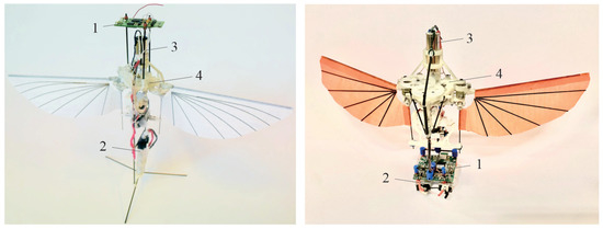
Figure 1.
The robot COLIBRI in two different configurations. 1: Flight control board. 2: LiPo battery. 3: Main DC motor. 4: Flapping mechanism.
Various changes have been brought to the electromechanical parts of the robot to improve its autonomy [10]. Thanks to efficient aerodynamics and improved transmission, its measured specific mechanical power is around 135 W/kg, which is not far from that of a natural hummingbird [11], but the current limit to autonomy is that the mass of the existing robotic hummingbird is still about twice the mass of their natural counterpart with the same wing span [12].
The initial version of the COLIBRI robot used a Micro MWC Flight Control Board from Hobbyking with a clock of 16 MHz and a six-axis IMU (three-axis gyro and three-axis accelerometer), for a weight of 1.8 g. This board includes a proprietary algorithm for attitude reconstruction named DMP (Digital Motion Processor). A new control board has been developed including an ARM processor with a clockspeed of 168 MHz and two IMU sensors, one with six axes and one with nine axes, including a magnetometer. The board also includes a Bluetooth link, for a total weight of 1.4 g. It is briefly described in Appendix C. The IMUs are particularly critical components in view of the noisy environment due to the flapping of the wings.
1.2. Attitude Reconstruction
Attitude determination is a generic problem in satellites, the autopilots of aircraft and drones of various types, robotics, and biomechanics. The technology used depends on the application; our interest lies in the low-cost, low-weight MEMS inertial sensors (IMU) which are widely available. They are characterized by a low resolution, high noise, and time drift, and the problem consists of combining the output of a three-axis accelerometer unit with the output of a three-axis gyro to obtain a reasonably accurate, drift-free attitude estimate. The problem is particularly complicated for the flapping-wing robot because of the strong periodic disturbance generated by the flapping of the wings (see Appendix A; the amplitude of the periodic sensor signals generated by the flapping wings is one order of magnitude larger than the cycle-averaged signal that we intend to capture). The purpose of this paper is not to report on the huge body of literature available on attitude reconstruction (e.g., [13,14,15,16,17,18,19,20,21]), but rather to extract the part of it which is most appropriate for the specific problem of a flapping-wing robot near hovering. Two aspects are particularly relevant:
(i) Most models proposed in the literature use quaternion kinematics for attitude estimation. However, near hovering, the longitudinal and lateral dynamics of the flapping-wing robot are nearly decoupled and can be treated as independent [22,23,24]. As a result, the attitude determination can be handled independently as a one-dimensional problem in the longitudinal (pitch) and the lateral (roll) directions.
(ii) Since the lift generation process produces a strong disturbance in the robot dynamics, it is expected that including the robot dynamics in the attitude determination, as advocated by [21], may improve the estimator.
The two approaches below will be considered:
(i) The complementary filter takes advantage of the hovering assumption (absolute acceleration = 0), according to which the accelerometer provides the direction of the gravity vector in the robot frame.
(ii) A full-state dynamic observer (implemented as a Kalman filter) includes robot dynamics in the attitude estimation. In addition to the robot attitude, this approach also reconstructs the linear velocity of the robot, allowing it to enforce hovering without external additional information.
The results of this study are expected to be confirmed by upcoming flight tests, where special attention will be paid to the trade-off between noise rejection and the stability margins. Measured flapping noise data are presented in the Appendix A, Appendix B and Appendix C,together with a description of a new, proprietary flight control board.
2. Flight Dynamics
2.1. Cycle-Averaged Longitudinal Dynamics
Previous studies have shown that the hummingbird robot can be modeled as a rigid body. Additionally, due to the weak coupling between the longitudinal (pitch) and the lateral (roll) dynamics, they may be assumed to be uncoupled and modeled separately. The present discussion will, therefore, be limited to the longitudinal axis; a similar model applies to the lateral axis. Additionally, since the flapping frequency is high compared to the robot dynamics near hovering, the latter may be based on cycle-averaged aerodynamic forces and moments; a similar approach was followed by [22,23,24]. The rapid change in the aerodynamic moment as well as the lift and drag forces during a flapping cycle appear as noise. These are particularly important in the longitudinal axis because the aerodynamic forces are not self-equilibrated. On the contrary, the aerodynamic forces along the lateral axis are self-balanced within a flapping cycle (due to left-right symmetry). Delft university has developed a flapper drone with four wings which is also self-equilibrated on the longitudinal axis [25]; this architecture increases the lift with the so-called clapandfling mechanism and it considerably reduces the flapping disturbance. However, such a morphology does not exist in nature.
The pitch and roll axes of COLIBRI are naturally unstable; they must be controlled actively; the yaw axis is naturally stable and can be treated separately.
The main damping mechanism is the flapping of the wings. It can be modeled by a point force proportional to the velocity of the center of drag (CD) located above the center of mass (Figure 2). The position of the center of drag is estimated at a quarter chord from the leading edge at mid-wing. The position of the center of mass (CG) is obtained either from CAD or from static equilibrium tests.
where the constant K is a linear function of the flapping frequency. u is the axial velocity and q is the pitch angular velocity. This model was validated with a set of pendulum experiments (Figure 3) [1,26].
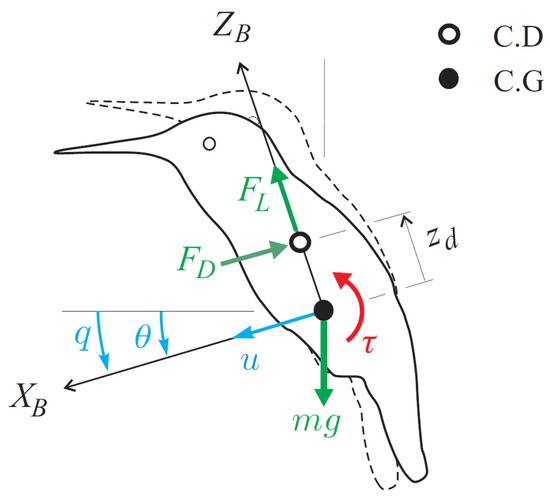
Figure 2.
Longitudinal (pitch) model of the robot near hovering. Coordinate system, force, and moment diagram.
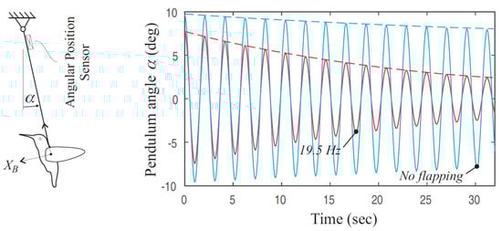
Figure 3.
Left: Pendulum test for determining the damping constant K. Right: Typical free response with and without flapping. K increases linearly with the flapping frequency.
Referring to Figure 2, the longitudinal dynamics near hovering is governed by the Newton–Euler equations. Newton’s equation reads
where m is the mass of the robot, u is the velocity of the center of mass, is the pitch angle (assumed small, so that and ), and is the pitch velocity. L is the lift (follower) force; at hovering, its vertical component balances the gravity force , and the component along the body axis is . is the drag force along ; from Equation (1), and .
Similarly, the Euler equation reads
where is the moment of inertia about the center of mass; is the drag torque with and . can be estimated with a pendulum experiment similar to that of Figure 3 with the pendulum axis aligned on the center of mass. Note that direct and fairly accurate measurements of and are available while the cross-coupling terms and result from a model and are less accurate; the distance between the center of mass and the center of drag is not known accurately. is the aerodynamic control torque that, in our robot, is obtained by the rotation of the control bars as explained below. The latter are operated by servos which can be modeled as first-order systems, so that the actual control torque is related to the requested torque (output of the controller) by
where T is the time constant of the servo. In state space form, the cycle-averaged longitudinal dynamics read
where and are always negative and and are negative if , that is, if the center of drag is above the center of mass, and they are positive if . Similar considerations apply to the lateral dynamics and will not be repeated. All the simulations reported below have been performed with the data listed in Appendix B.
2.2. Cycle-Averaged Control Torques
The wings consist of reinforced membranes attached to two orthogonal bars [1]; the leading edge bars drive the wings while the control bars (orthogonal to the leading edge bars in neutral position) create the control torques via a mechanism called wingtwistmodulation introduced by [5]; moving the control bars sideways from the neutral position induces a reorganization of the airflow, changing the location of the center of pressure along the wing, creating a roll torque while keeping the lift nearly unchanged. Similarly, moving the control bars forward or backward produces a pitch torque without altering the lift. It has been shown that the cycle-averaged roll and pitch moments are nearly independent (i.e., the pitch moment is independent of the position of the roll actuator and vice versa) and that they do not significantly affect the lift force for a given flapping frequency [1]. This confirms that the cycle-averaged axial and lateral dynamics can be treated independently. The cycle-averaged control torques ( in the foregoing model) are nearly proportional to the control bars angles which are the output of the control servos.
The aerodynamics of the flapping-wing robot at hovering is extremely complex and is out of the scope of this paper. The time histories of the lift, drag, and aerodynamic torque (measured by attaching the robot to a load cell) exhibit strong harmonic components at frequencies multiple times the flapping frequency, with peak amplitudes significantly larger than their cycle-averaged values (Appendix A). For the present discussion, these periodic disturbances appear as input noise, the drag noise d is added to the right-hand side of Equation (2), and the torque noise is added to the right-hand side of Equation (3). These periodic disturbances enter at the input of the system and induce strong vibrations which propagate to the inertial unit (IMU). This process, which belongs to the physics of the flapping flight, was judged important enough to justify to include two IMUs with different saturation thresholds in the design of the control board.
3. Stabilization
The open-loop longitudinal dynamics is unstable and the poles configuration depends strongly of on the value of . For (center of drag above the center of mass), the system has two unstable oscillatory poles and two poles on the negative real axis (Figure 4). If one considers the system a SISO system with the control torque as input and the pitch angle as output, the system can be stabilized with a PD compensator, . This adds a zero in the open-loop system; Figure 4 shows the root locus as a function of the proportional gain . The position of the closed-loop poles corresponding to , 15 mm, and is indicated in red [1].
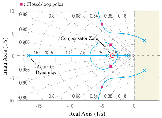
Figure 4.
Root–locus plot trajectories as a function of the proportional feedback gain for PD control of the robot with and mm. The open-loop poles and zero are in blue. The red squares indicate the closed-loop poles location obtained with .
The PD compensator discussed above looks satisfactory; however, the pitch angle is not directly available because the IMU MEMS unit consists of three rate gyros measuring the roll–pitch–yaw angular velocity in the robot frame and the three components of the specific acceleration s = a−g, i.e., the absolute vector acceleration of the IMU unit minus the gravity vector . In hovering, , and the specific acceleration indicates the position of the gravity vector in the robot frame, from which the robot attitude (roll–pitch) can be calculated:
For the 1-D model considered here, if the IMU is located at a distance of the center of mass ( if the IMU is above the center of mass and if it is below),
At hovering, in absence of noise, . Note that the component is subject to the flapping noise due to the periodic variation in the lift force within a cycle. As a result, near hovering, may be a more accurate estimator.
Considering the system equation, Equation (5), the output equation relating the sensor output to the state vector reads
The gyros are subjected to drift and one cannot rely on them in low frequency. On the contrary, MEMS accelerometers are sensitive to noise in high frequency, and it is only at hovering, when the absolute acceleration is close to zero, that the specific acceleration can be translated into the gravity vector from which the robot attitude can be deduced. In the following sections, we consider two ways of combining the gyros and the accelerometers’ information to improve the attitude estimation: the complementary filter and the dynamic state observer.
4. Complementary Filter
Prior to the complementary filter, the IMU outputs are passed into a second-order Butterworth low-pass filter with a corner frequency for the gyros and for the accelerometers (Figure 5); the choice in and is discussed below.
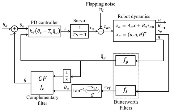
Figure 5.
Block diagram of the longitudinal stability control loop with a complementary filter. is the requested control torque, is the position of the servo actuator acting on the control bars, and is the actual torque produced by the flapping wings, including the periodic components discussed earlier.
The complementary filter consists of blending the high-frequency information contained in the gyro signals with the low-frequency information contained in the accelerometers’ output. In the 1-D model considered here, this means that the gyro output q is first integrated to provide the pitch angle , which is high-pass filtered (HP) to eliminate the low-frequency components responsible for the drift. The accelerometer output is used to estimate the pitch angle which, in turn, is low-pass filtered (LP) to eliminate the high-frequency noise. The two filters are such that together they constitute an all-pass filter (HP + LP = 1). Assuming second-order Butterworth filters,
where is the corner frequency of the complementary filter. The block diagram of the stability control loop with a complementary filter is shown in Figure 5. One sees that in the output of the gyro, after passing into the low-pass filter , is used directly for the D part of the PD compensator and it is also integrated to result in at the input of the complementary filter. The choice in the order of the filter and its cut-off frequency is critical because it introduces a delay in the feedback loop, which can have a detrimental effect on the system stability. In our study, we found that a second-order Butterworth filter with Hz is a good compromise. The component of the accelerometer unit is also low-pass filtered with a cut-off frequency before feeding the complementary filter. The choice of is less critical than that of , provided that is larger than the corner frequency of the complementary filter; Hz and Hz were found satisfactory.
The control system of Figure 5 can be looked at as a SISO system with unit feedback, with input and output ; Figure 6 shows the Nichols plot for the following values of the filter frequencies: Hz, Hz, and Hz (the system is linearized according to ). The stability margins are, respectively: phase margin PM = 66 ( Hz) and gain margin GM = 8 dB ( Hz). The figure also shows the Nichols plot when the Butterworth filter on the gyro signal is removed (), showing the impact of this filter on stability. The control loop may be improved by adding a compensator on the pitch angle error (we will return to this in the following section). The complementary filter does not produce a direct estimate of the axial velocity u, and an additional measurement system is needed to enforce hovering. Because the axial velocity u is one of the state variables in Equation (5), enforcing hovering with on-board measurements only is possible if one uses a full-state dynamic observer, as discussed below.
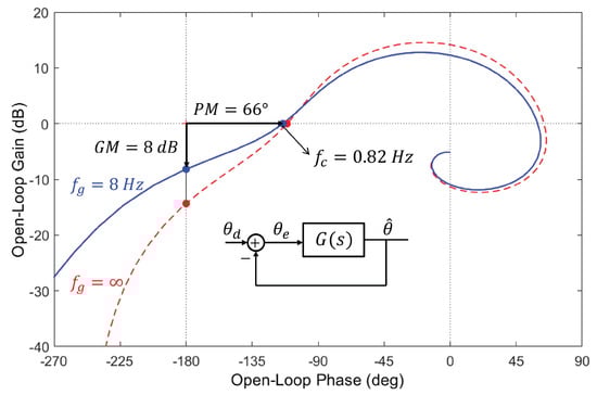
Figure 6.
Complementary filter: Nichols plot for Hz, Hz, and Hz. In dashed lines, without filter on the gyro output ().
5. Full-State Dynamic Observer
If one takes into account the flapping of the wings, the axial dynamics of the robot can be written in the classical state space form:
where . The matrices A and B are provided in Equation (5).
w represents the system noise produced by the flapping of the wings, , where d is the drag force and is the aerodynamic pitch torque due to the flapping of the wings. Both are periodic; they are documented in Appendix A.
The output equation, Equation (10), is rewritten:
where (output of the accelerometers and the gyros) and v is the sensor noise, of which we know little.
An alternative to the complementary filter consists of reconstructing the state with a full-state dynamic (Luenberger) observer (Figure 7). The reconstructed state is solution of
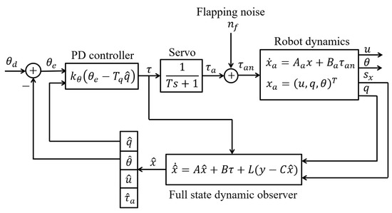
Figure 7.
Block diagram of the longitudinal stability control loop with a full-state dynamic observer. The symbols have the same meaning as in the previous figure.
The error follows the equation
The observer gain matrix L is chosen to achieve adequate filtering properties of the IMU signals from the gyro and the accelerometer. Since the PD regulator may be looked at as full-state feedback, the separation principle applies and the closed-loop poles consist of two decoupled sets, corresponding to the full-state feedback regulator (PD in this case) and the full-state observer. The closed-loop stability is guaranteed provided the observer is stable (i.e., the eigenvalues of have negative real parts).
5.1. Plant Noise and Sensor Noise
Although the flapping noise does not fulfill the assumption of white noise, the Kalman filter theory is a very convenient tool to generate a reasonable gain matrix L; various forms are assumed for the system and measurement noise until appropriate filtering properties are achieved.
Equation (5) describes the cycle-averaged dynamics of the robot. If one considers the drag force and pitch torque variations during the flapping cycle as noise, it becomes
where d is the drag force and is the pitch torque induced by the flapping of the wings. Time histories of d and are shown in Appendix A, from which the variance of (N/kg) and (N/kg·m) can be estimated (the components of the plant noise are expressed in different units; in SI units, their ratio is 100).
The sensor noise covariance matrix may be estimated from the zero-acceleration output of the accelerometers and the zero-rate output of the gyros, available from the data sheet of the IMU sensor, respectively, 0.30 m/s2 and 0.085 rad/s, leading to (m/s2)2 and (rad/s). Thus, the ratio is .
5.2. Kalman Filter
According to the foregoing discussion, we assume the following form for the plant noise W and the sensor noise V:
where is a design parameter. A small value of indicates that low noise measurements may be trusted. Note that only the ratio between V and W matters (multiplying both matrices by a scaler leads to the same gain matrix L). Since the measurement noise acts as an excitation in the observer error equation, amplified by the observer gain matrix, noisy measurements require moderate gains in the observer.
Figure 8 shows the observer poles for three values of , respectively, 1, 10, and 100. The figure includes the poles of the PD regulator shown earlier in Figure 4. The value of has been used in what follows.
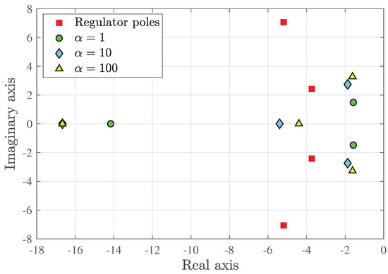
Figure 8.
Observer poles for 1, 10, and 100 (the pole on the left side of the real axis is common to all values of ).The regulator poles of Figure 4 are also shown.
The robustness of the observer deserves some attention: The matrices A, B, and C in the observer equation constitute a model of the real system. As discussed earlier, the elements of the system matrix (, , etc.) can be experimentally determined fairly accurately; a larger uncertainty exists in because the location of the center of drag is not known accurately (even the concept of center of drag is oversimplified). A parametric study with reasonable variation in the system parameters led to small changes in the observer poles.
Figure 9 compares the Nichols plot of the transfer function between and for the Kalman filter () and the complementary filter of Figure 6. The behavior can be further improved by inserting a compensator in the direct loop. Figure 10 illustrates this for the compensator consisting of a P + I plus a Lead compensator aiming to improve the control bandwidth while keeping good stability margins:
where , , Hz, , Hz, , and Hz. The crossover frequency raises to Hz and the stability margins to, respectively, PM and GM =16.4 dB. Such a compensator can also be used (with appropriate tuning of the parameters) for the complementary filter.
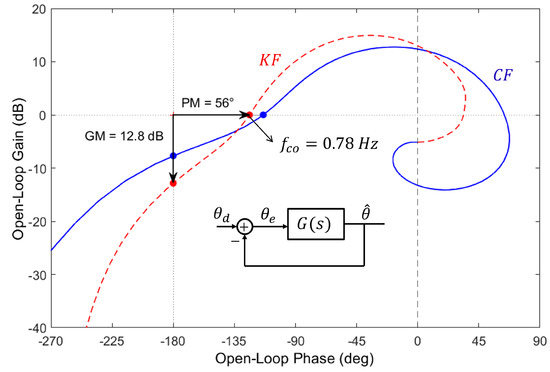
Figure 9.
Nichols plot for the Kalman filter (KF) () and the complementary filter (CF) of Figure 6.
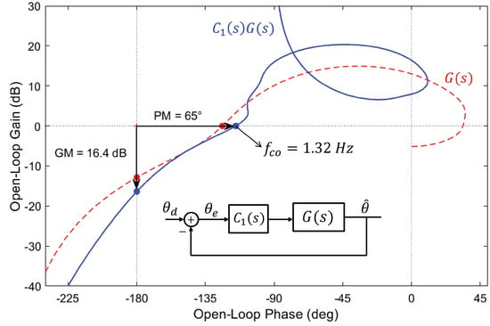
Figure 10.
Kalman Filter (): Effect of adding the compensator consisting of a P + I and a Lead compensator.
Figure 11 shows the time history of the pitch angle estimate for a step response of . The smooth line (blue) corresponds to the case where the flapping noise is ignored; the noisy curve (red) accounts for the drag and pitch torque noise shown in Appendix A. The time–history integration includes a saturation of the control torque 200 g·mm (2 N·mm).
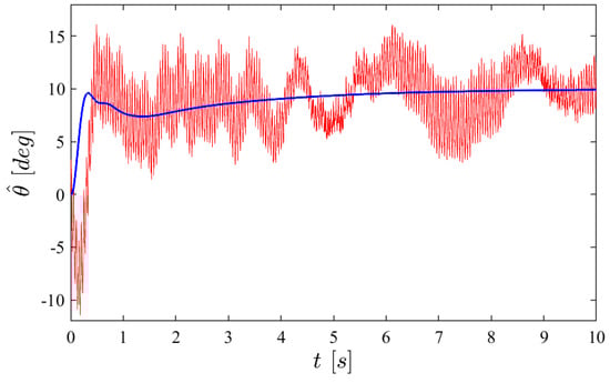
Figure 11.
Step response of : with (in red) and without (in blue) flapping drag d and pitch torque noise .
5.3. Hovering
Unlike the complementary filter which estimates the pitch angle , the full-state dynamic observer also reconstructs the linear velocity which allows direct control of the robot’s hovering and, more generally, of the trajectory. Figure 12 shows the cascade structure of the control system; is the desired axial speed and is the reconstructed one; is the velocity error. The transfer function between and is that of a SISO system. The compensator transforms the velocity error into a pitch angle demand . According to Equation (2), in steady state (at equilibrium, ), the drag force is balanced by the tilting of the lift force, . It follows that . Figure 13 shows the Nichols plot of the transfer function when a P + I compensator is used:
where with and rad/s.
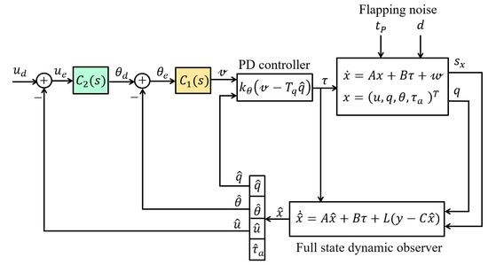
Figure 12.
Cascaded control on the linear velocity u. The flapping noise includes the drag d and the pitch torque .
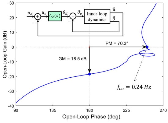
Figure 13.
Nichols plot of the linear velocity loop with the P + I compensator .
Figure 14 shows the time history of the step response when a speed of m/s is requested. The figure shows the reconstructed velocity and the reconstructed pitch angle when the flapping noise is ignored (smooth curve in blue) and when the flapping noise (drag and pitch torque) is included (in red). Here again, the time–history integration includes a saturation of the control torque 200 g·mm (2 N·mm). Figure 11 and Figure 14 illustrate the trade-off between noise attenuation and stability margins: further low-pass filtering is possible, but at the expense of reducing the stability margins. This aspect will be investigated carefully in future flight tests.
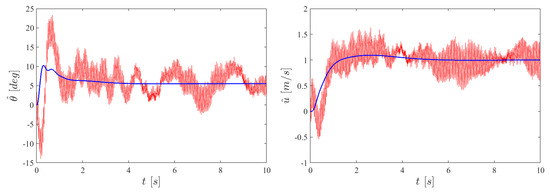
Figure 14.
Step response with a requested speed of m/s, with (red) and without (blue) flapping noise. Right: reconstructed speed . Left: corresponding reconstructed pitch angle .
6. Conclusions
The paper investigates numerically the control and attitude reconstruction of a flapping-twin-wing robot near hovering in presence of the strong noise generated by the flapping of the wings. The axial (drag) force and the pitch moment components of the periodic flapping noise are characterized from experimental data (provided in Appendix A). Two approaches are considered for attitude reconstruction from IMU data: complementary filter and full-state dynamic observer (Kalman filter). The complementary filter takes advantage of the hovering assumption to reconstruct the pitch angle (for closed-loop stability), but it does not provide access to the longitudinal velocity (for hovering). On the contrary, the full-state observer reconstructs the pitch angle and the longitudinal velocity, which can be controlled without additional information from an external source. Numerical simulations (based on data of the COLIBRI robot) show that the full-state observer provides a solution for the control of the trajectory, but there is a trade-off between the residual oscillations due to the flapping wings and the stability margins of the closed-loop attitude control, making the complete cancellation of the oscillations difficult. On-board implementation and flight tests will be conducted as soon as the various subsystems of the robot, including the new proprietary control board described in Appendix C, are assembled and ready for flight.
Author Contributions
Conceptualization, A.P., Y.F., L.W., L.B. and H.W.; software, Y.F. and L.W.; validation, A.P., Y.F., L.W., L.B., H.W. and K.W.; writing—original draft preparation, A.P.; writing—review and editing, A.P., Y.F. and K.W.; supervision, A.P. All authors have read and agreed to the published version of the manuscript.
Funding
This research received no external funding.
Institutional Review Board Statement
Not applicable.
Informed Consent Statement
Not applicable.
Data Availability Statement
Data are contained within the article.
Acknowledgments
The authors wish to thank Ir. Gert Deboers from Dekimo n.v. for his careful work in the manufacturing of the control board and his availability and help in the initial phase of programming.
Conflicts of Interest
The authors declare no conflict of interest.
Abbreviations
The following abbreviations are used in this manuscript:
| ARM | Advanced RISC Machine |
| CF | Complementary Filter |
| DARPA | Defense Advanced Research Projects Agency |
| DMP | Digital Motion Processor |
| FFT | Fast Fourier Transform |
| GM | Gain Margin |
| HP | High-Pass Filter |
| IMU | Inertial Measurement Unit |
| KF | Kalman Filter |
| LP | Low-Pass Filter |
| MCU | Micro Controller Unit |
| MEMS | Micro Electromechanical System |
| PD | Proportional plus Derivative |
| PI | Proportional plus Integral |
| PM | Phase Margin |
| RMS | Root Mean Square |
| SI | International System Units |
| SISO | Single Input Single Output |
Appendix A. Flapping Disturbance
Appendix A.1. Lift
Figure A1 shows the time history of the lift force when the flapping frequency is 22.3 Hz and the lift is 23.3 g (0.229 N). The figure also shows the detail of one cycle and the FFT decomposition showing the harmonic content of the time history (unfortunately, the lack of synchronization of the experimental set-up between the flapping mechanism and the force measurement does not allow us to identify the upstroke and the downstroke in the force recording over one cycle). The figure shows that the lift distribution of a membrane wing mounted on a flexible leading edge bar is extremely complicated, far more than that of the flat-plate wing shown in [27]. The RMS value of the lift force is 126 g (1.24 N).
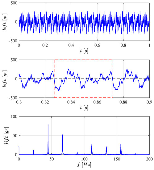
Figure A1.
From top to bottom: Time history of the lift force when the flapping frequency is 22.3 Hz and the cycle-averaged lift is 23.3 g. Detail of one cycle. FFT transform showing the harmonics, multiple times the flapping frequency.
Appendix A.2. Pitch Torque
Figure A2 shows the time history of the actual aerodynamic torque. Here, again, the signal is periodic and extremely complicated, with peak values up to 30 times the maximum value of the pitch and roll control torques which are limited near ±200 g·mm (2 N·mm) [1]. In the cycle-averaged model, this periodic disturbance torque enters at the input of the system and induces strong vibrations that propagate to the inertial units [Equation (16)]. The RMS value of the aerodynamic torque is 0.0273 Nm (2780 g·mm).
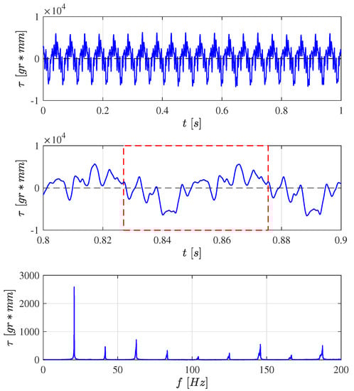
Figure A2.
From top to bottom: Time history of the aerodynamic torque when the flapping frequency is 20.8 Hz with the servo actuator near neutral position (the average torque is 17.8 g·mm). Detail of one cycle. FFT transform showing the harmonics, multiple times the flapping frequency.
Appendix A.3. Drag
Similarly, Figure A3 examines the drag force d when the flapping frequency is 19.9 Hz. The peak values are up to 20 times the average lift. In the cycle-averaged model, this produces a periodic disturbance force d in the right-hand side of Equation (16) that excites the robot and propagates to the IMU. Note that the average value of 2.6 g indicates that the wing behavior is not exactly symmetrical between the upstroke and the downstroke, producing a net axial force. At hovering, such a bias force has to be balanced by tilting the robot by . The RMS value of the aerodynamic drag is 0.985 N (100 g).
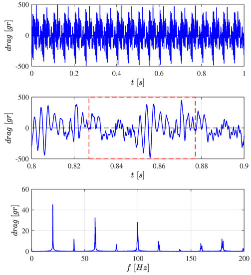
Figure A3.
From top to bottom: Time history of the drag force d when the flapping frequency is 19.9 Hz; the average drag is 2.6 g. Detail of one cycle. FFT transform showing the harmonics, multiple times the flapping frequency.
Appendix B. COLIBRI Parameters Used in the Dynamics Model
All simulations reported in this paper are based on data taken from [1]; they are listed in Table A1.

Table A1.
COLIBRI parameters for the body dynamics model.
Appendix C. Flight Control Board
Figure A4 shows the new flight control board. The manufacturing was contracted to Dekimo Leuven n.v. The size is 25 × 26 mm and the weight is 1.6 g. The main components, their reference number, and their communication protocol are shown in Figure A5. The board allows us to directly control the three servos for attitude control and the main motor for lift production; a Bluetooth module communicates with the ground station.
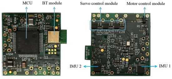
Figure A4.
Both sides of the 25 × 26 mm control board. Weight: 1.6 g.
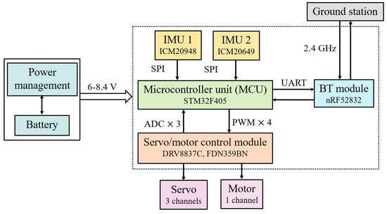
Figure A5.
Main components of the control board.
Because of the critical role played by the attitude sensing, due to the flapping noise, the board was provided with two IMU units:
- (i)
- IMU-1: ICM-20948. 9-axis. Accelerometer Full Scale Range ±16 g. Gyro Full Scale Range ±2000 deg/s. Magnetometer Full Scale Range ±6900 μT.
- (ii)
- IMU-2: ICM-20649. 6-axis. Accelerometer Full Scale Range ±32 g. Gyro Full Scale Range ±4000 deg/s.
The data acquisition rate is 500 Hz (three accelerometers and three gyros). The MCU unit, STM32F405, has a clock frequency of 168 MHz. The nominal battery input is 7.4 V; it is regulated to supply the main motor (6 V), the servo actuators (4.2 V–6 V), and the IC components (3.3 V and 1.8 V). Additional I2C and SPI ports are reserved for future optical sensors.
References
- Roshanbin, A. Design and Development of a Tailless Robotic Hummingbird. Ph.D. Thesis, Université Libre de Bruxelles, Dept Control Engineering and System Analysis, Brussels, Belgium, September 2019. [Google Scholar]
- Roshanbin, A.; Altartouri, H.; Karasek, M.; Preumont, A. COLIBRI: A Hovering Flapping Twin-Wing Robot. Int. J. Micro Air Veh. 2017, 9, 270–282. [Google Scholar] [CrossRef]
- Roshanbin, A.; Abad, F.; Preumont, A. Kinematic and Aerodynamic Enhancement of a Robotic Hummingbird. AIAA J. 2019, 57, 4599–4607. [Google Scholar] [CrossRef]
- Available online: https://www.youtube.com/watch?v=-5-o9tvbziE (accessed on 21 May 2023).
- Keennon, M.T.; Klingebiel, K.R.; Won, H.; Andriukov, A. Development of the nano hummingbird: A tailless flapping wing micro air vehicle. In Proceedings of the 50th AIAA Aerospace Sciences Meeting Including the New Horizons Forum and Aerospace Exposition, Nashville, TN, USA, 9–12 January 2012; pp. 1–24. [Google Scholar]
- Phan, H.V.; Park, H.C. Insect-inspired, tailless, hover-capable flapping-wing robots: Recent progress, challenges, and future directions. Prog. Aerosp. Sci. 2019, 111, 100573. [Google Scholar] [CrossRef]
- Phan, H.V.; Aurecianus, S.; Au, T.K.L.; Kang, T.; Park, H.C. Towards Long-Endurnce Flight of an Insect-Inspired, Tailess, Two-Winged, Flapping-Wing Flying Robot. IEEE Robot. Autom. Lett. 2020, 5, 5059–5066. [Google Scholar] [CrossRef]
- Xiao, S.; Hu, K.; Huang, B.; Deng, H.; Ding, X. A Review of Research on the Mechanical Desig of Hoverable Flapping Wing Micro-Air Vehicles. J. Bionic Eng. 2021, 18, 1235–1254. [Google Scholar] [CrossRef]
- Floreano, D.; Wood, R.J. Science, technoloy and the future of small autonomous drones. Nature 2015, 521, 460–466. [Google Scholar] [CrossRef] [PubMed]
- Preumont, A.; Wang, H.; Kang, S.; Wang, K.; Roshanbin, A. A Note on the Electromechanical Design of a Robotic Hummingbird. Actuators 2021, 10, 52. [Google Scholar] [CrossRef]
- Ellington, C.P. The novel aerodynamics of insect flight: Applications to micro-air vehicles. J. Exp. Biol. 1999, 202, 3439–3448. [Google Scholar] [CrossRef] [PubMed]
- Greenwalt, C.H. Hummingbirds; Dover: New York, NY, USA, 1990. [Google Scholar]
- Madgwick, S.O.H. An efficient orientation filter for inertial and inertial/magnetic sensor arrays. Rep.-Univ. Bristol 2010, 25, 113–118. [Google Scholar]
- Mahony, R.; Hamel, T.; Pflimlin, J.-M. Nonlinear Complementary Filter on the Special Orthogonal Group. IEEE Trans. Autom. Control 2008, 53, 1203–1218. [Google Scholar] [CrossRef]
- Euston, M.; Coote, P.; Mahony, R.; Kim, J.; Hamel, T. A Complementary Filter for Attitude Estimation of a Fixed-Wing UAV. In Proceedings of the 2008 IEEE/RSJ International Conference on Intelligent Robots and Systems, Nice, France, 22–26 September 2008. [Google Scholar]
- Sabatelli, S.; Galgani, M.; Fanucci, L.; Rocchi, A. A Double Stage Kalman Filter for Orientation Tracking with an Integrated Processor in 9-D IMU. IEEE Trans. Instrum. Meas. 2013, 62, 590–598. [Google Scholar] [CrossRef]
- Min, H.G.; Jeung, E.T. Complementary Filter Design for Angle Estimation Using MEMS Accelerometer and Gyroscope. Available online: https://www.academia.edu/6261055/Complementary_Filter_Design_for_Angle_Estimation_using_MEMS_Accelerometer_and_Gyroscope (accessed on 21 May 2023).
- Narkhede, P.; Poddar, S.; Walambe, R.; Ghinea, G.; Kotecha, K. Cascaded Complementary Filter Architecture for Sensor Fusion in Attitude Estimation. Sensors 2021, 21, 1937. [Google Scholar] [CrossRef] [PubMed]
- Gebre-Egziabher, D.; Hayward, R.C.; Powell, J.D. Design of Multi-sensor Attitude Determination Systems. IEEE Trans. Aerosp. Electron. Syst. 2004, 40, 627–649. [Google Scholar] [CrossRef]
- Lefferts, E.J.; Markley, L.; Shuster, M.D. Kalman filtering for spacecraft attitude estimation. In Proceedings of the AIAA Aerospace Sciences Meeting (AIAA-82-0070), Orlando, FL, USA, 11–14 January 1982. [Google Scholar]
- Yang, Y.; Zhou, Z. Attitude determination: With or without spacecraft dynamics. Adv. Aircr. Spacecr. Sci. 2017, 4, 335–351. [Google Scholar]
- Van Breugel, F.; Regan, W.; Lipson, H. From Insects to Machines. IEEE Robot. Autom. 2008, 15, 68–74. [Google Scholar] [CrossRef]
- Ristroph, L.; Ristroph, G.; Morozova, S.; Bergou, A.J.; Chang, S.; Guckenheimer, J.; Wang, Z.J.; Cohen, I. Active and passive stabilization of body pitch in insect flight. J. R. Soc. Interface 2013, 10, 20130237. [Google Scholar] [CrossRef] [PubMed]
- Teoh, Z.E.; Fuller, S.B.; Chirarattananon, P.; Pérez-Arancibia, N.O.; Greenberg, J.D.; Wood, R.J. A Hovering Flapping-Wing Microrobot with Altitutde Control and Passive Upright Stability. In Proceedings of the 2012 IEEE/RSJ International Conference on Intelligent Robots and Systems, Vilamoura, Portugal, 7–12 October 2012; pp. 3209–3216. [Google Scholar]
- Karásek, M.; Muijres, F.T.; De Wagter, C.; Remes, B.D.; De Croon, G.C. A tailess aerial robotic flapper reveals that flies use torque coupling in rapid banked turns. Science 2018, 361, 1089–1094. [Google Scholar] [CrossRef] [PubMed]
- Altartouri, H.; Roshanbin, A.; Andreolli, G.; Fazzi, L.; Karásek, M.; Lalami, M.; Preumont, A. Passive stability enhancement with sails of a hovering flapping twin-wing robot. Int. J. Micro Air Veh. 2019, 11, 1–9. [Google Scholar] [CrossRef]
- Dickinson, M.H.; Lehman, F.-O.; Sane, S.P. Wing rotation and the aerodynamic basis of insect flight. Science 1999, 284, 1954–1960. [Google Scholar] [CrossRef] [PubMed]


Disclaimer/Publisher’s Note: The statements, opinions and data contained in all publications are solely those of the individual author(s) and contributor(s) and not of MDPI and/or the editor(s). MDPI and/or the editor(s) disclaim responsibility for any injury to people or property resulting from any ideas, methods, instructions or products referred to in the content. |
© 2023 by the authors. Licensee MDPI, Basel, Switzerland. This article is an open access article distributed under the terms and conditions of the Creative Commons Attribution (CC BY) license (https://creativecommons.org/licenses/by/4.0/).