Abstract
High-precision industrial manipulators are essential components in advanced manufacturing. Model-based feedforward is the key to realizing the high-precision control of industrial robot manipulators. However, traditional feedforward control approaches are based on rigid models or flexible joint models which neglect the elasticities out of the rotational directions and degrade the setpoint precision significantly. To eliminate the effects of elasticities in all directions, a high-precision setpoint feedforward control method is proposed based on the output redefinition of the extended flexible joint model (EFJM). First, the flexible industrial robots are modeled by the EFJM to describe the elasticities in joint rotational directions and out of the rotational directions. Second, the nonminimum-phase EFJM is transformed into a minimum-phase system by using output redefinition. Third, the setpoint control task is transformed from Cartesian space into joint space by trajectory planning based on the EFJM. Third, a universal recursive algorithm is designed to compute the feedforward torque based on the EFJM. Moreover, the computational performance is improved. By compensating the pose errors caused by elasticities in all directions, the proposed method can effectively improve the setpoint control precision. The effectiveness of the proposed method is illustrated by simulation and experimental studies. The experimental results show that the proposed method reduces position errors by more than 65% and the orientation errors by more than 62%.
1. Introduction
Industrial robot manipulators have been applied in many manufacturing fields, such as assembly and welding. However, it is still a great challenge to expand robotics applications to high-precision machining processes due to the low accuracy [1]. Various feedback control methods such as PID control, sliding mode control [2], and observer-based control [3] have been adopted to improve the end effector setpoint control precision of industrial robots. However, it is difficult to achieve high-precision control with only feedback controllers owing to the complex nonlinear dynamics of industrial manipulators. Alternatively, model inversion-based feedforward control [4] is an effective approach that solves the problem by compensating the nonlinear dynamics. A nonlinear PD controller plus feedforward compensation was proposed for rigid robots to achieve the finite-time stabilization of the tracking error [5]. To improve the robustness-to-payload uncertainty, an intelligent feedforward controller using a neural network and fuzzy logic was designed for a two-link robot manipulator [6].
Nevertheless, the above feedforward control methods are based on the rigid robot model, which neglects the flexible deformations of manipulators. Actually, the flexibilities of some compliant transmission elements such as harmonic drives and cycloidal gears have significant effects on setpoint control performance [7]. In response to the problem, the flexible joint model (FJM) was proposed, which models the joint as a linear torsional spring [8]. Based on the FJM, a feedforward minimum-time position control method was proposed to avoid oscillation of a flexible robot [9]. Based on comprehensive modeling of the flexible joint and an extended generalized Maxwell friction model, an adaptive feedforward controller was designed to compensate the nonlinear dynamics of transmissions [10].
However, only the elasticities in revolute directions are considered in the FJM, which neglects the elasticities out of the rotational plane. In practice, modern industrial manipulators tend to have a slender design and lightweight materials. As a result, the flexible deformations out of the rotational plane caused by links and bearings are unneglectable, especially for high-speed and heavy-load manipulators [11]. Hence, the flexible joint model can not accurately describe a modern industrial robot. To improve the model accuracy, an extended flexible joint model (EFJM) was proposed [12] which can describe not only the elasticities in rotational planes but also the elastic deformations out of the plane. Then, the EFJM was validated on a modern industrial manipulator, and the results showed that the EFJM can greatly improve the model accuracy [13]. Thus, feedforward control based on the EFJM is a prospective way to improve the control precisions of flexible industrial manipulators.
Nevertheless, the EFJM possesses a differential nonflat characteristic, which is a great challenge for the feedforward controller design [14]. The feedforward control problem of a minimum-phase EFJM was solved by using differential algebraic equation (DAE) theory; thus, the tracking performance was improved significantly [12]. However, the EFJM is minimum phase only in special configuration. In most cases, the EFJM is a nonminimum-phase system [15]. A nonminimum-phase system possesses unstable internal dynamics; thus, the traditional feedforward control method cannot give a bounded solution [16]. To obtain a bounded feedforward input, a continuous DAE optimization solver and a discretized DAE optimization solver were proposed to solve the feedforward control problem of an EFJM with three degrees of freedom (DOFs) [17].
However, numerical optimization was adopted in the above methods due to the limitation of being nonminimum phase. Consequently, the existing methods have a heavy burden of calculation which is unacceptable for industrial robots with high DOFs. Moreover, the above methods are all based on analytic dynamic equations, which are difficult to obtain for complex manipulators. Thus, a high-precision feedforward control method with reasonable computational burden for general complex flexible industrial manipulators should be further explored.
To improve the setpoint control precision and reduce the computational burden, a new feedforward control approach based on the output redefinition of the EFJM is proposed for flexible industrial robots in this paper. Firstly, the output of the EFJM is redefined to transform the EFJM into a minimum-phase system. Thus, the limitation of the unstable internal dynamics is eliminated. Secondly, the joint trajectory is planned based on the kinematics and statics equations of the EFJM. Thus, the pose error caused by elasticity is compensated, and the setpoint problem is transformed into joint space. Finally, a universal feedforward torque computation algorithm for the EFJM is designed to reduce the calculation burden. The simulation and experimental studies demonstrate that the proposed method improves the control precision and computational efficiency remarkably.
2. Problem Formulation
2.1. Extended Flexible Joint Model
Lightweight design has been widely adopted in modern industrial robot manipulators, which causes complex mechanical elasticity in all directions. However, the traditional flexible joint model describes the joint by using a torsional spring, which can only model the joint flexibilities in rotational directions. In view of the problem, the EFJM was proposed to describe the elasticities of modern industrial robots more accurately [12].
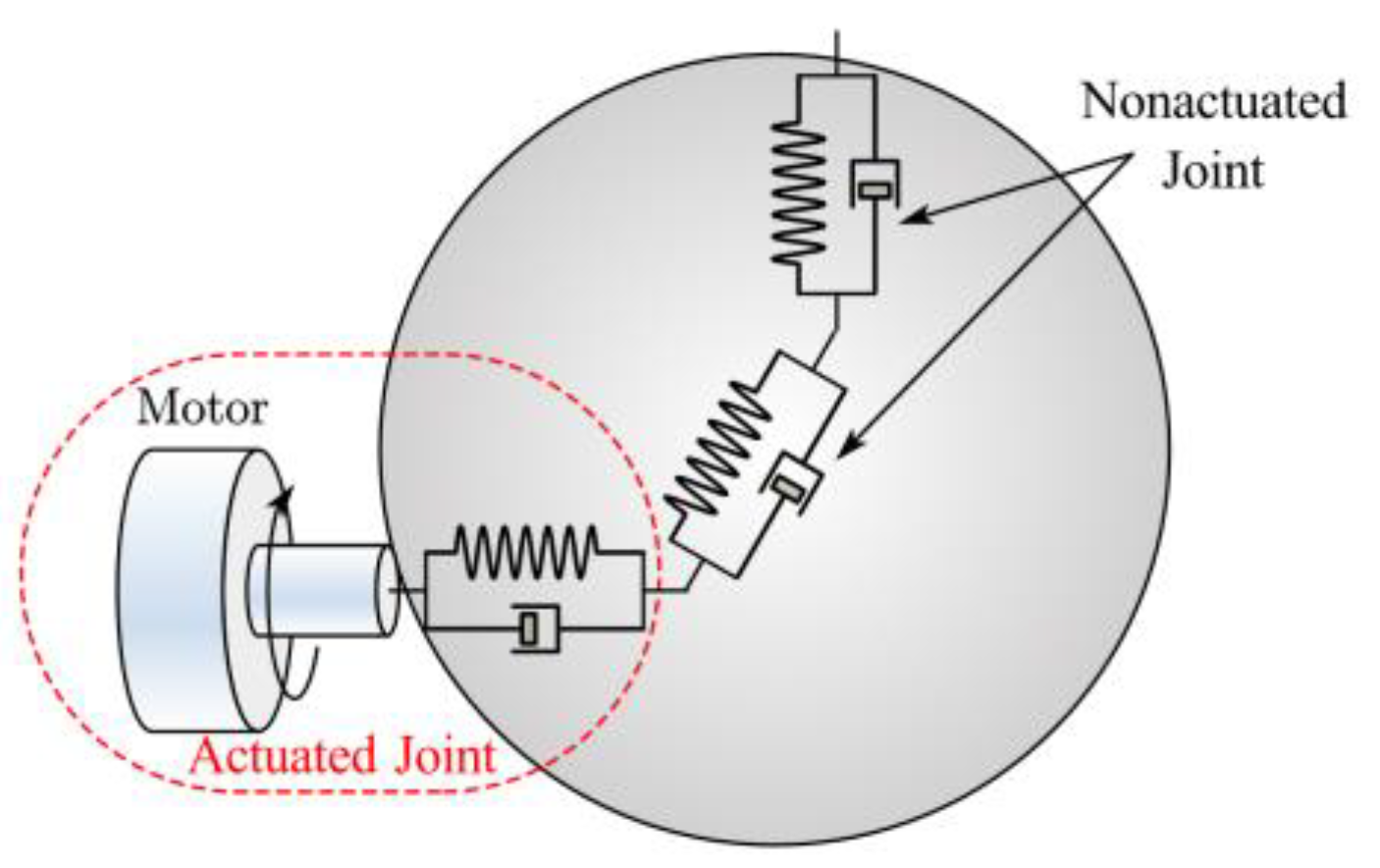
The extended flexible joint robot model is a lumped-parameter model consisting of a serial kinematic chain of rigid bodies. The rigid bodies are connected with extended flexible joints which consist of actuated joints and nonactuated joints. An example of an extended flexible joint is shown in Figure 1. The actuated joint consists of a motor, transmission, and a spring damping system, describing the elasticity in the rotational direction. The nonactuated joint uses a spring–damper pair to describe the elasticity out of the rotational plane caused by bearings, tools, and links. Consequently, the EFJM can describe the elasticities in all directions; thus, the model accuracy is improved significantly.
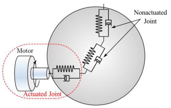
Figure 1.
An example of an extended flexible joint.
Assuming the weight of the load is known, the EFJM of a robot can be obtained by using the bottom-up approach in [13]. During the modeling process, the number and location of nonactuated joints should be determined by making a compromise between model accuracy and complexity. Then, the equations of dynamics can be derived by using Lagrange equations.
where , , and are the actuated and nonactuated joint angular position vectors, respectively; and are the motor angular position vector; denotes the gear ratio matrix; and are the friction torque vectors of the link side and motor side, respectively; is the inertia matrix of the robot; is the Coriolis and centripetal torque vector; and is the gravity torque vector, where . . denotes the inertia diagonal matrix of the motor side. is the motor torque vector, i.e., the control input. Since the flexible deflections are small, the flexibilities are modeled by linear springs and dampers in this paper. Then, the elastic torque vectors and are expressed as:
where and denote the stiffness and damping matrices in actuated and nonactuated directions, respectively. Consequently, the elasticity deformations of the manipulator are divided into two parts: elasticity deformation in the actuated direction and in the nonactuated direction .
Partitioning the generalized coordinates into actuated and nonactuated coordinates, the link-side dynamics (1) can also be separated into two parts:
where the dependency on the generalized coordinate and its derivate is dropped for readability.
Obviously, the submatrices , and satisfy the following properties [7].
Property 1: Inertia matrix is symmetric and positive definite, i.e., , .
Property 2: and satisfy the following equations:
Property 3: Both gravity torque and its partial derivative with respect to are formed by trigonometric functions of the variable . Thus, there exist positive constants and such that:
where denotes the Euclidean norm of a vector or matrix.
Correspondingly, the reasonable assumptions are made as follows:
Assumption 1.
The damping matrix in the nonactuated direction is not zero.
Assumption 2.
The stiffness matrix of the nonactuated joint satisfies:
where denotes the minimum eigenvalue of .
2.2. Setpoint Control Problem
Using the forward kinematics of the robot, the orientation and position of the end effector can be expressed as:
The objective of point-to-point feedforward control is to design a control torque such that the end effector of manipulator systems (1), (2), and (9) moves to a desired constant pose at specified time from initial configuration , with all elastic deformations being compensated and all closed-loop signals remaining bounded.
The EFJM is a differentially nonflat system; thus, the feedforward control input relies on the stable solution of the internal dynamics. However, from motor torque to end effector pose , the system is nonminimum phase in most cases, i.e., the solution of the internal dynamics may be unbounded [16]. Thus, it is difficult to compute the feedforward torque directly based on the end effector pose.
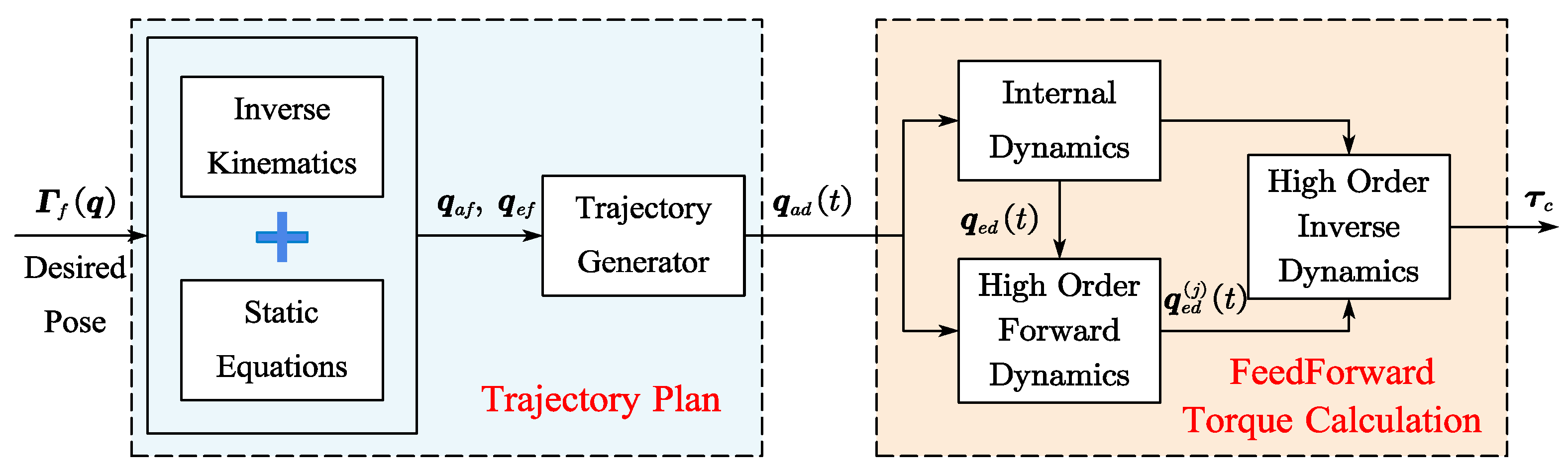
In response to the above limitations, the proposed feedforward setpoint control method consists of two steps, as shown in Figure 2. Firstly, the system output is redefined as , and the reference trajectories of actuated joint positions are planned. Secondly, the nominal feedforward torque is computed by using the EFJM of the robot based on the reference actuated joint trajectories . Then, the desired point-to-point motion of the end effector is accomplished indirectly.
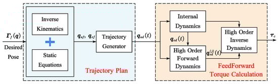
Figure 2.
Procedure of proposed feedforward control method.
3. Controller Design
To achieve high-precision setpoint control of the end effector, an output-redefinition-based feedforward control method is proposed for the EFJM in this section.
Firstly, it is proven through Lyapunov theorem that the EFJM is transformed into a minimum-phase system by redefining the system output as . Secondly, the reference trajectory is planned in joint space based on the kinematics and static equation of the EFJM. Thus, the pose error caused by the flexibility deformations is compensated accurately. Finally, the feedforward control torque for the EFJM is calculated by using the recursive dynamics algorithms; thus, the computational burden is further reduced.
3.1. Output Redefinition of EFJM
As mentioned above, from motor torque to end effector pose , the EFJM is nonminimum phase in most cases. Consequently, an unbounded solution of internal dynamics may be obtained, leading to unbounded feedforward torques. To stabilize the internal dynamics and overcome the limitation of being nonminimum phase, the system output is redefined as in this section. Then, the stability of internal dynamics is analyzed.
Differentiating the first equation of (5) twice yields:
where .
Neglect the damping of actuated joints and consider the motor dynamics (2); then, the input output relationship of the EFJM is obtained.
where is the system input.
Clearly, the dynamics of the unactuated joints coordinates are the internal dynamics of the EFJM.
Let the output and ; then, the zero dynamics of the EFJM are obtained as:
We can conclude from Assumption 2 [7] that system (13) has an equilibrium , which satisfies:
The Lyapunov candidate function is chosen as:
where denotes an energy-like function which is defined as:
where means the gravitational potential energy of robot which satisfies:
Obviously, is the stationary point of function, as the partial derivative of w.r.t is:
Taking the partial derivative of (18) with respect to again yields:
According to Property 3 and the assumption , the right side of (19) is positive definite. Hence, is the global minimum point for . Then, we obtain , , and .
The time derivative of is:
According to (12) and (14), we obtain:
Recalling Property 2 yields:
According to Assumption 1, is negative semi-definite if and only if . What is more, the function is a radially unbounded positive semi-definite function. We can conclude from the Krasovskii theorem that the equilibrium is globally asymptotically stable. Thus, the original unstable internal dynamics are transformed into new, stable internal dynamics by choosing actuated joint position vector as system out. The limitation of the nonminimum-phase EFJM can be avoided.
3.2. Trajectory Planning in Joint Space
It is obvious that the flexible deformations of unactuated joints lead to a pose error of the end effector; thus, the inverse kinematics problem of the extended flexible joint model should first be studied in trajectory planning. For convenience, assume that the robot is a six-DOFs serial joint robot manipulator and away from the singularity. Obviously, the dimension of is larger than six; thus, the kinematic relation (9) of the EFJM is noninvertible. In order to obtain a unique solution, additional constraints on unactuated joints should be considered. In a static condition, the unactuated joint positions are determined by gravity torque; thus, the following equations should be satisfied:
The desired joint positions and can be obtained by solving the above nonlinear algebraic equations with a numerical solver which requires an initial guess. Considering the elastic deformations in nonactuated directions are small, the solution of the inverse kinematics of the rigid model can be chosen as the initial guess.
Based on the initial configuration and desired configuration , the joint position reference trajectories and its derivatives can be planned in joint space by adopting a trajectory planning algorithm with continuous jerk profile.
Through the accurate trajectory tracking of , the end effector accomplishes the desired point-to-point motion. Thus, the setpoint control problem is transformed to the trajectory tracking problem in joint space.
3.3. Calculation of Feedforward Torque
According to (2) and (3), the feedforward torque can be obtained as:
The elastic torque vector in actuated direction and its derivatives and can be expressed as:
where . The above equations can be calculated efficiently by using the recursive Newton–Euler algorithm (RNEA) [18] and elastic joint Newton–Euler algorithm (EJNEA) [19], respectively.
where , , , , and , and EJNEA3 means the reduced version of the EJNEA, returning .
Note that the nonactuated joint angular positions , velocities , accelerations , jerks , and snaps are required. Since the stability of zero dynamics is ensured, and can be obtained by solving the internal dynamics (12) using numerical integration solvers based on initial condition .
Then, can be obtained efficiently by solving the following linear equations:
where , , and . and are obtained using the composite rigid body algorithm (CRBA) [20]. Let ; then, can be obtained through adopting the RNEA.
Similarly, and can be obtained by solving the following equations:
where . The nonlinear terms and are calculated by adopting the and as follows:
According to (3), the motor position and velocity are derived as:
By now, all required variables in (25) are known; thus, the feedforward torque calculation is completed, and the total procedure is summarized as follows:
Step 1. Solve the internal dynamics (12) using an ODE solver to obtain ;
Step 2. Compute matrices using the ;
Step 3. Compute using the RNEA and solve (32) to obtain ;
Step 4. Compute using the and solve (34) to obtain ;
Step 5. Compute using the and solve (35) to obtain ;
Step 6. Compute , , and using the , , and , respectively;
Step 7. Compute and using (38) and (39);
Step 8. Compute feedforward torque using (25).
Remark 1.
The elastic deformations in nonactuated directions are compensated by solving (23), while the elasticities in actuated directions are compensated in the feedforward torque calculation algorithm. Thus, the proposed method can further improve the control precision.
Remark 2.
It is time consuming to solve the internal dynamics (12) through numerical integration. However, the traditional stable inversion methods [17] are based on numerical optimization which needs to solve the internal dynamics repetitively. In contrast, the internal dynamics need to be solved only once in the proposed calculation algorithm since the EFJM is transformed into a minimum-phase system. Thus, the computational burden is remarkably reduced.
Remark 3.
The proposed calculation algorithm does not require the analytic expression of the robot; thus, it can be applied to general open-chain robots easily.
4. Simulation and Experimental Results
Considering the disturbance, noise, and the parameter uncertainties of actual manipulators, a PID feedback controller is employed in simulations and experiments to improve the robustness and to avoid the drift of tracking errors. Since only the motor side is equipped with position sensors for most industrial manipulators, the motor torque command is designed as:
where is the feedforward torque, and are constant controller gain matrices. The reference motor trajectories are obtained using (38).
4.1. Simulation Results
- (1)
- Example 1: A planar robot
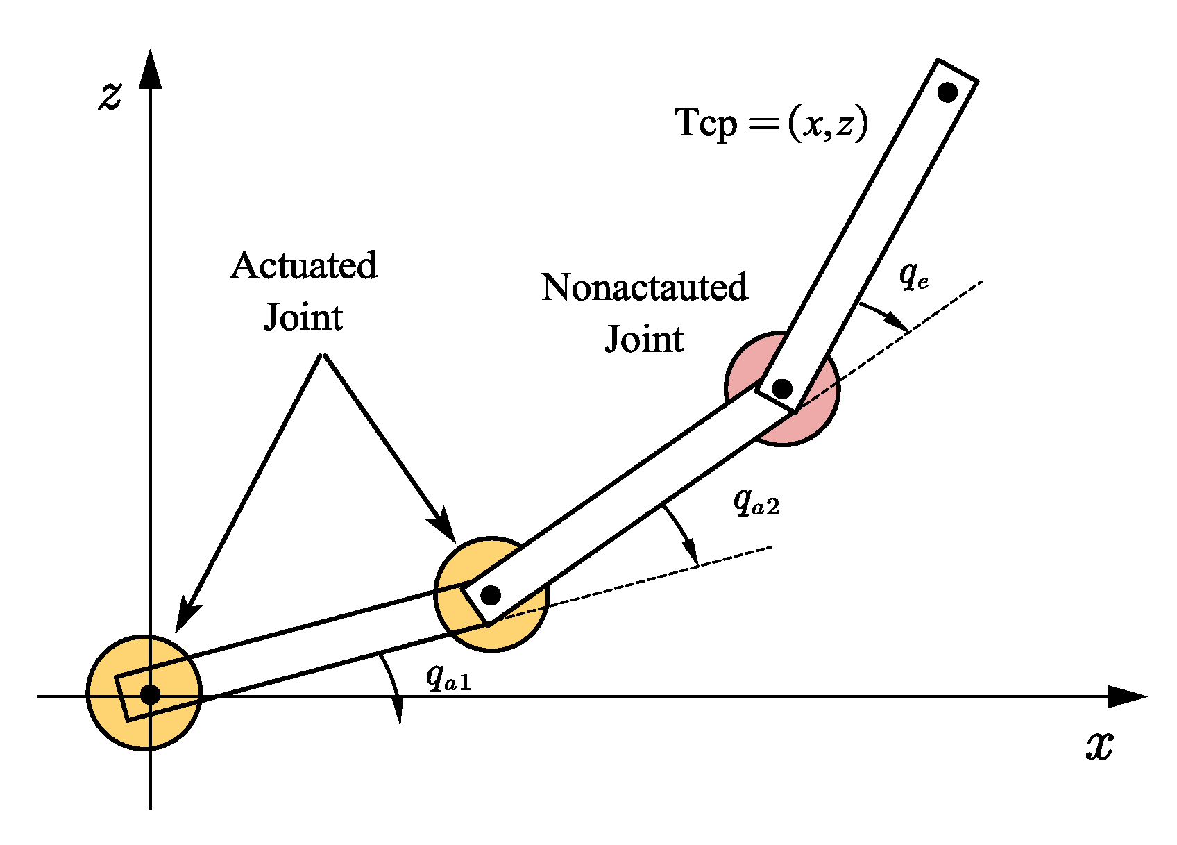
To validate the superiority of the proposed output-redefinition-based feedforward control approach (ORFF), simulations using the ORFF, the traditional FJM-based feedforward approach (FJMFF) [21], and the continuous DAE optimization solver (CDAEOS) [17] are carried out on a planar robot in this section. As shown in Figure 3, the EFJM of this planar robot has three rigid bodies, two actuated joints, and one nonactuated joint. The dynamic parameters of each link in this planar robot are shown in Table 1 where the link parameters include length , inertia , mass , center of mass , and joint parameters including stiffness , damping , and motor inertia .
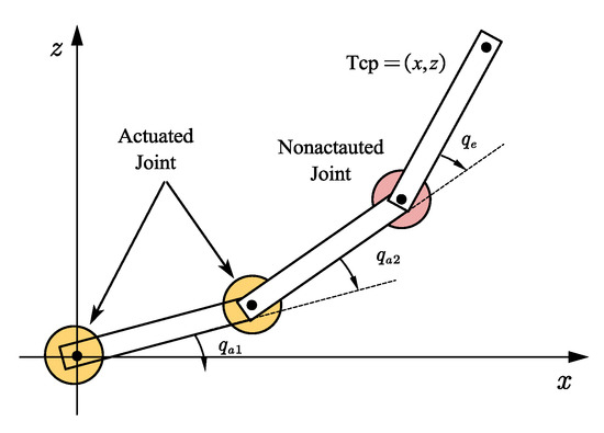
Figure 3.
The EFJM of planar robot.

Table 1.
Dynamic parameters of planar robot.
To show the efficiency of the proposed computation algorithm clearly, the feedforward torques are solved using three methods on an Intel i5-10400 PC with 16 G RAM. The step size is selected as 1 ms in the simulation. The tip of the robot moves from to in 0.5 s, 1 s, and 2 s. The execution times and setpoint control errors of the three methods are shown in Table 2.
Table 2.
Solving times and control errors of the three methods in simulation, example 1.
As indicated in Table 2, the setpoint control error of the proposed ORFF is significantly reduced compared with that of the FJMFF and CDAEOS under three conditions. When the moving time is 1 s, the control error of the ORFF is reduced by over 90% and 80% compared with that of the CDAEOS and FJMFF, respectively. On the other hand, the execution time of the ORFF is 4–5 times that of the FJMFF, while the execution time of the CDAEOS is much longer than that of the other two methods.
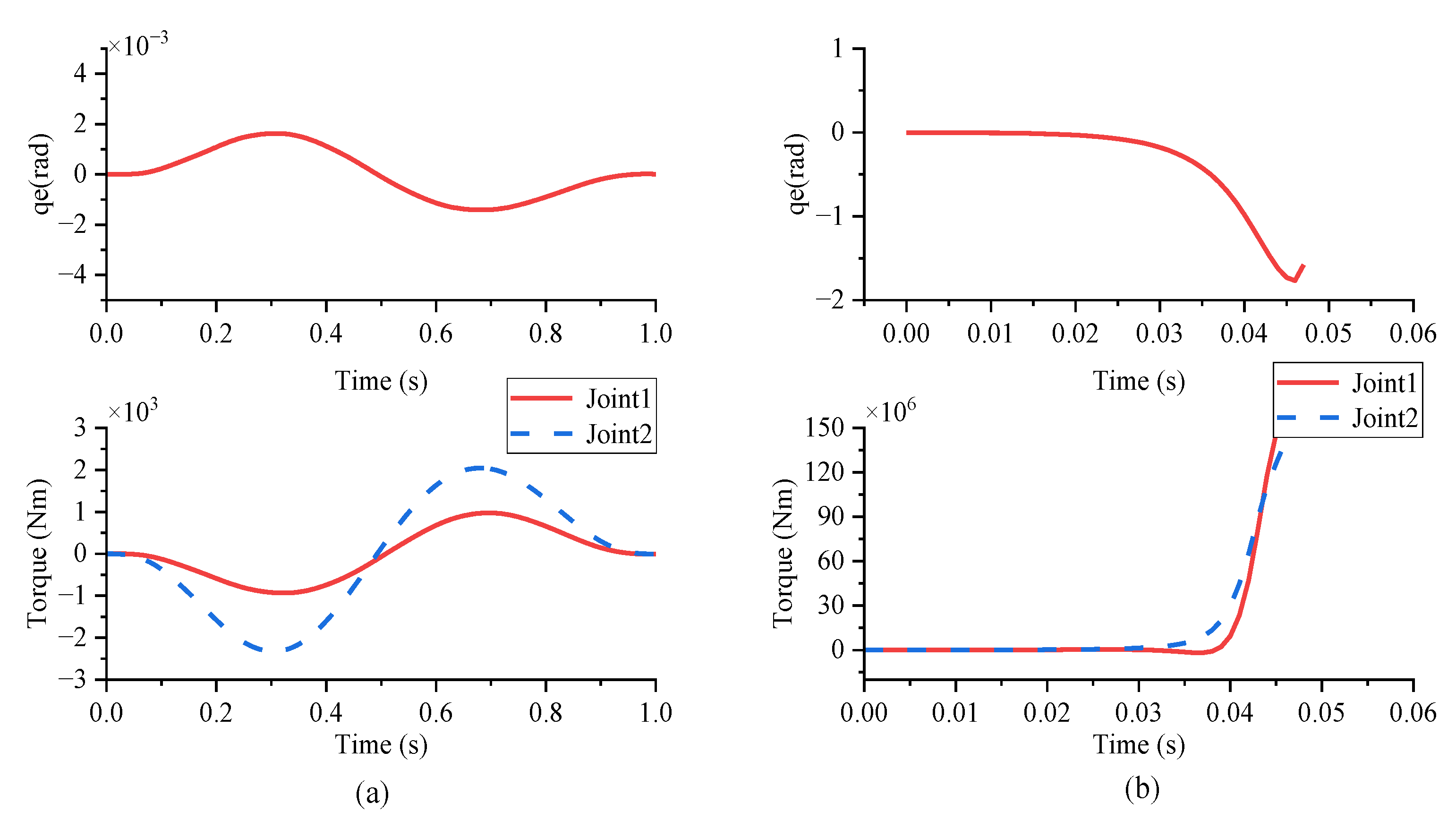
The bounded feedforward torques and nonactuated joint positions obtained by using the proposed ORFF are shown in Figure 4a. As a comparison, the feedforward torques are solved without output redefinition, and the results are shown in Figure 4b. It is obvious that the internal dynamics of the original EFJM system are unstable, and the feedforward torques are unbounded. Thus, the results in Figure 4 demonstrate that the system is transformed into a nonminimum-phase system by output redefinition.
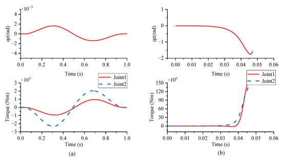
Figure 4.
Nonactuated joint positions and feedforward torques: (a) with output redefinition; (b) without output redefinition.
- (2)
- Example 2: Six DOFs Manipulator
To prove the proposed method can be applied to complex industrial manipulators, simulations are carried out on an EFORT ER7 robot with six DOFs. The dynamic parameters are shown in Table 3.
Table 3.
Dynamic parameters of ER7.
Firstly, simulations are carried out using the rigid model of ER7, where all elasticities are ignored. The traditional rigid-model-based feedforward method (RMFF) is used to control the robot, i.e., the feedforward torque in (40) is computed using the rigid robot model. The parameters of the PID controller are chosen as , , and , where . The target pose of the end effector is selected randomly in the task space, and 100-run simulations are carried out. The setpoint control root-mean-square errors (RMSEs) are shown in Table 4.
Table 4.
Setpoint control RMSEs of rigid model using RMFF.
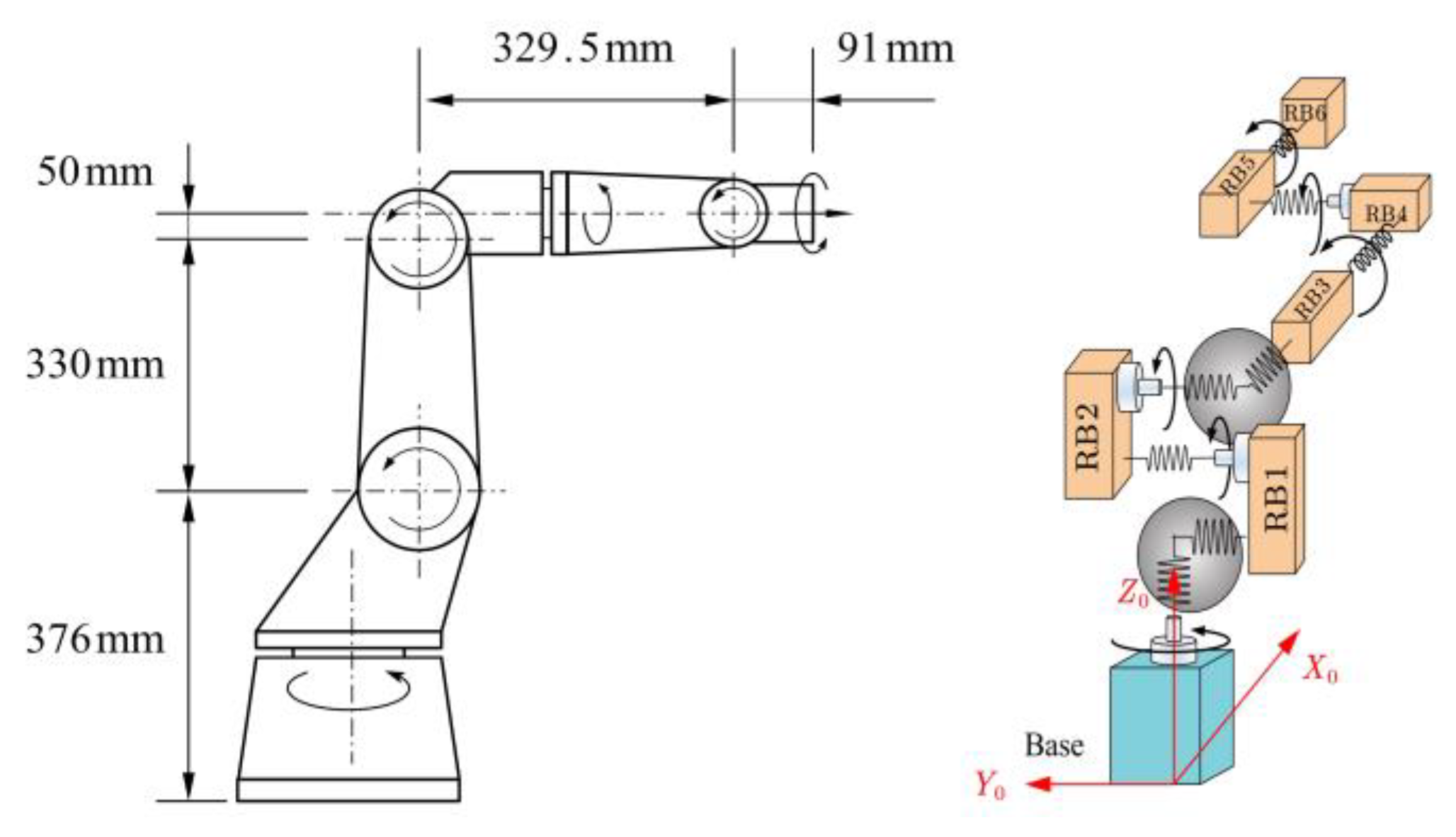
Secondly, simulations are carried out using the flexible model of ER7 with different load levels. The EFJM of ER7 with six actuated joints and two nonactuated joints is built as shown in Figure 5. The flexible parameters are shown in Table 5, where the two nonactuated joints are denoted by joints 1Y and 3Y.

Figure 5.
Geometric model and extended flexible joint model of EFORT ER7.
Table 5.
Parameters of extended flexible joints of ER7.
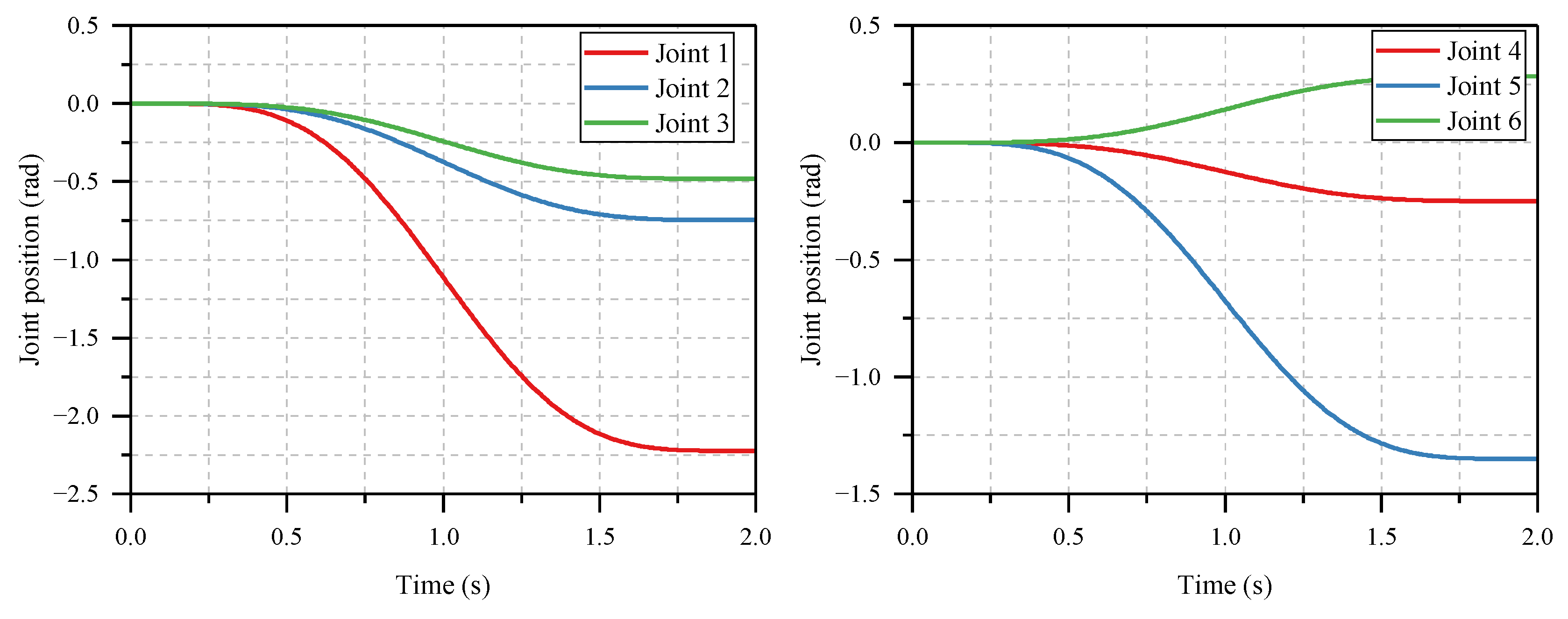
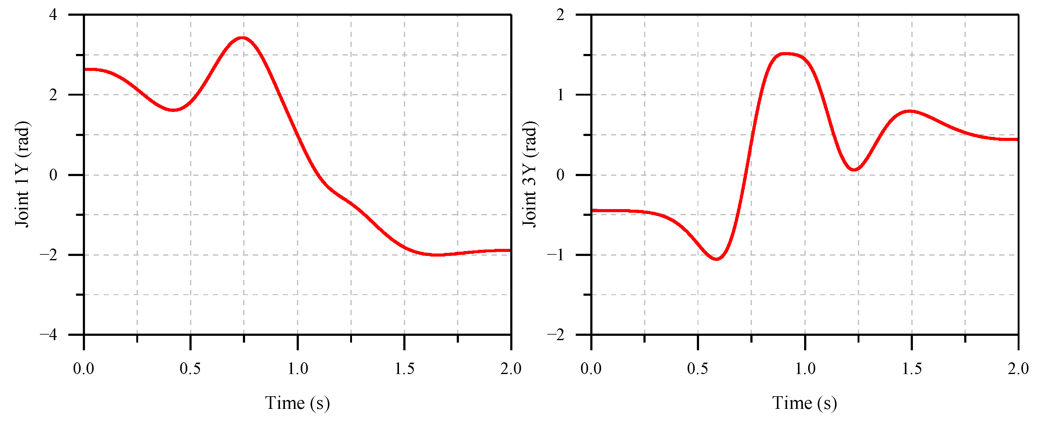
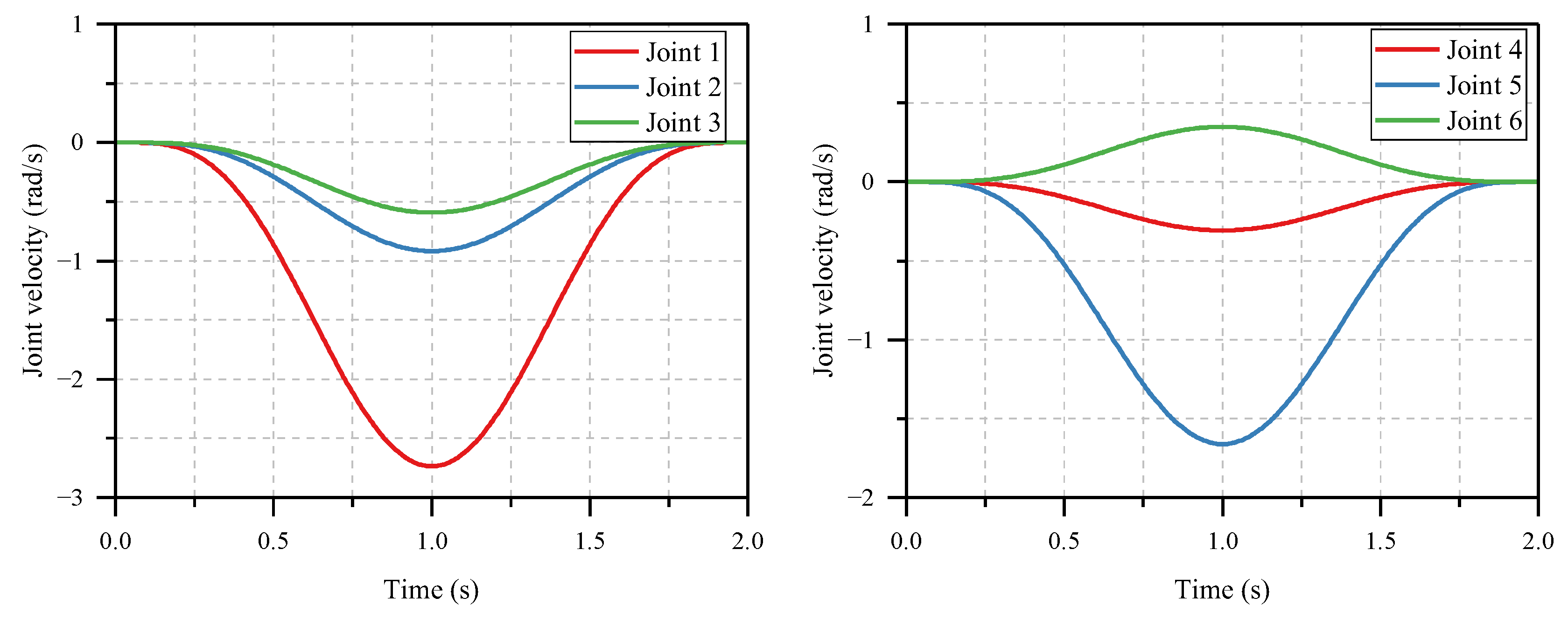
Similarly, 100-run simulations for ER7 are carried out by selecting the target end effector pose randomly. In order to demonstrate the improved performance of the proposed method under the different load conditions, the payload of the robot is set to 0 kg, 3 kg, and 6.5 kg, respectively. Since the model is too complicated for the CDAEOS to obtain a solution in reasonable time, only the traditional RMFF and FJMFF are adopted for comparison. The step size of the feedforward torque solver is 1 ms. The average execution times of the ORFF and FJMFF are 1.3457 s and 0.2554 s, respectively. The setpoint control RMSE of the ORFF and FJMFF are shown in Table 6, where the orientation error is given in the form of a Euler angle. The control results of the first group of simulations using the proposed ORFF under 6.5 kg payload are shown in Figure 6, Figure 7, Figure 8 and Figure 9. The actuated joint and nonactuated positions are shown in Figure 6 and Figure 7, respectively. The actuated joint velocities are shown in Figure 8. It can be seen that the nonactuated joint positions are bounded, which indicates that the internal dynamics are stable. Hence, bounded control torques are obtained by using the proposed ORFF method, as shown in Figure 9.
Table 6.
Setpoint control RMSEs of flexible model in simulation, example 2.
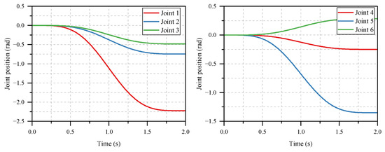
Figure 6.
Actuated joint positions in first group simulation under ORFF.
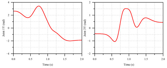
Figure 7.
Nonactuated joint positions in first group simulation under ORFF.
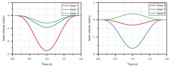
Figure 8.
Actuated joint velocities in first group simulation under ORFF.
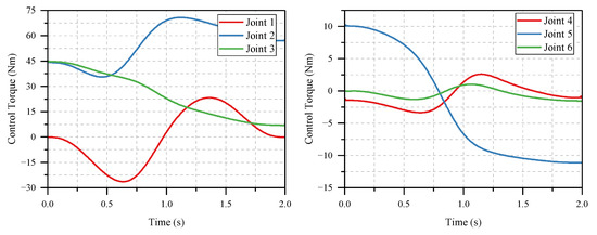
Figure 9.
Control torques in first group simulation under ORFF.
As shown in Table 5, the traditional RMFF can achieve a satisfactory control accuracy for a rigid robot model. However, the control accuracy of the RMFF is greatly reduced in a flexible robot model when the effects of elasticities are considered, as shown in Table 6. Although the FJM method can improve the control accuracy, it fails to achieve satisfactory results as it can only compensate the effects of elasticities in rotational directions. In contrast, the proposed ORFF method achieves optimal control precision since it can compensate the effects of elasticities in all directions. In addition, it can be seen that the control RMSE of the flexible model using the ORFF is at the same level as the control RMSE of the rigid model using the RMFF control method. This also indicates that the pose error caused by flexibilities are compensated accurately by using the ORFF. Moreover, by comparing the control accuracy under different load conditions, it can be seen that the improvement achieved by the ORFF is more evident under high-payload conditions.
4.2. Experimental Results
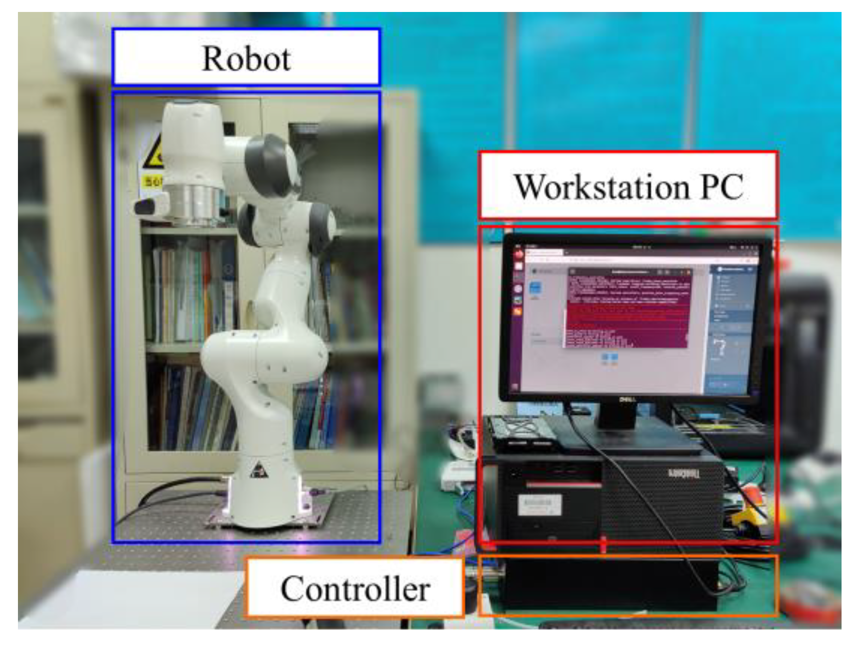
To further evaluate the effectiveness of the proposed feedforward control method, experiments are carried out using a Franka Emika Panda 7-DOF Manipulator. As shown in Figure 10, the experimental platform consists of the robot, its control unit, and a workstation PC. Based on ROS, the PC can send real-time torque commands at 1 kHz to the robot.
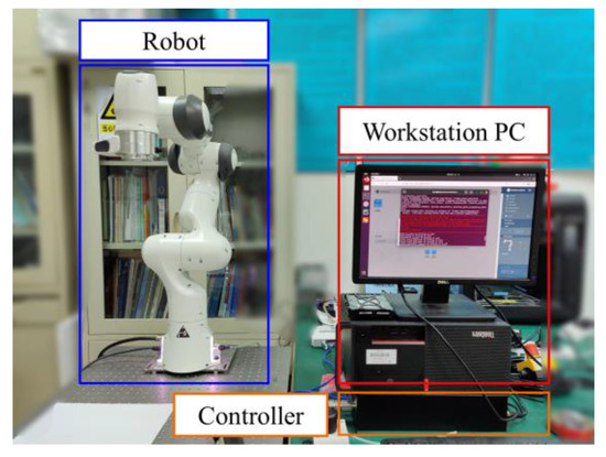
Figure 10.
Experimental platform.
In order to simulate the effect of the unactuated joint, the motor position of the third joint remains fixed. Then, the dynamics of the Panda can be described by the EFJM, as shown in Figure 11. The parameters of the extended flexible joints are identified through experiments, as shown in Table 7, where the unactuated joint is denoted by joint 3Y. The dynamic parameters of the Panda have already been identified [22].
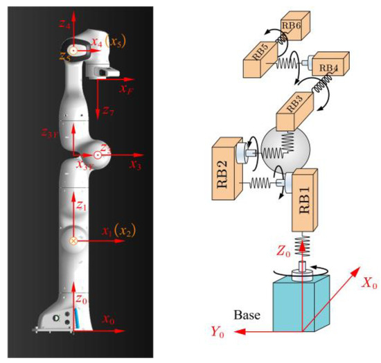
Figure 11.
Parameters and the EFJM of the Franka Emika Panda.
Table 7.
Parameters of extended flexible joints of the Panda.
In experiment, 25 target points are selected randomly in Cartesian space. Then, the ORFF and FJMFF are employed to control the robot combined with the PD controller. The parameters of the PD controller are shown in Table 8. Similarly, the CDAEOS is not employed in the experiments due to its heavy computational burden. The feedforward torques are solved offline, and the average execution times of the ORFF and FJMFF are 8.2552 s and 0.9884 s, respectively. The desired trajectories of the actuated joints are generated by using a smooth planning algorithm [23], and corresponding feedforward torques are computed. The setpoint control RMSEs of the two control methods are shown in Table 9. It can be seen that the RMSE of the proposed method is reduced significantly compared with that of the FJMFF. The position RMSEs of the proposed method decrease by 65%, 81%, and 92% in the x-, y-, and z-directions, respectively, and the orientation RMSEs decrease by 62%, 64%, and 71% in the three directions, respectively.
Table 8.
Parameters of PD controller in experiments.
Table 9.
Setpoint control RMSEs of two methods in experiments.
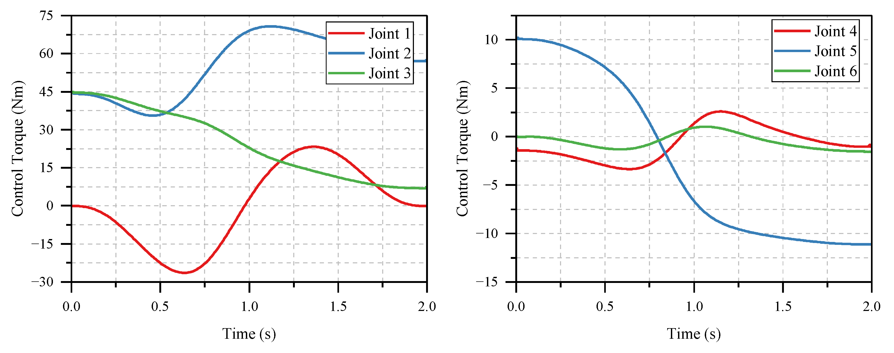
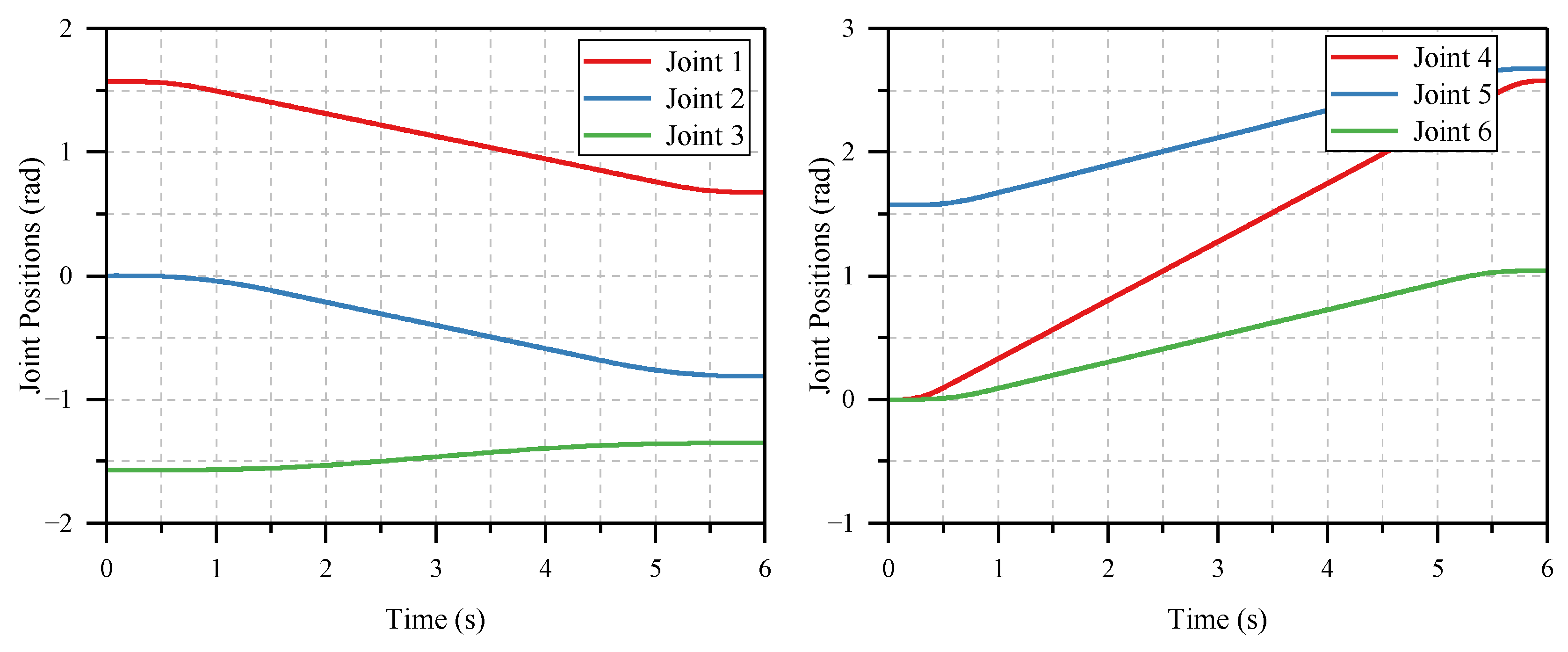
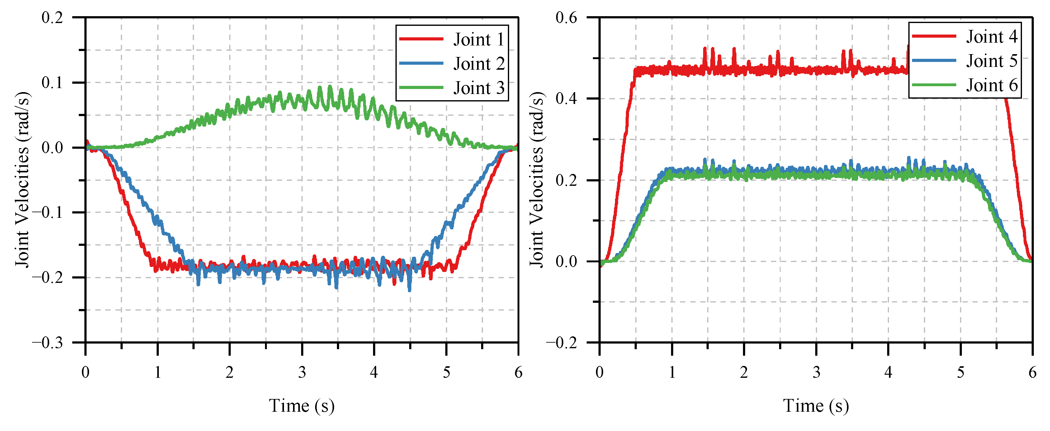
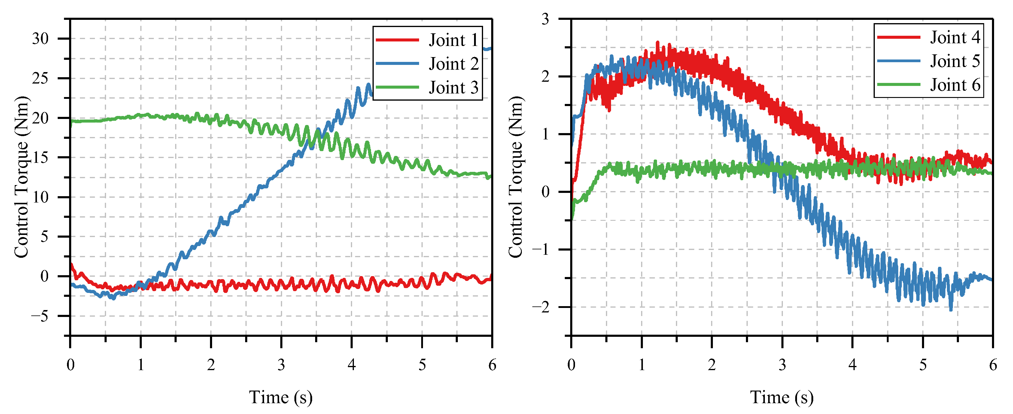
Figure 12, Figure 13 and Figure 14 show the control results of the first group of experiments under the proposed ORFF method. Figure 12 and Figure 13 show the actuated joint positions and velocities, respectively. The control torques using the proposed ORFF method are shown in Figure 14. It can be seen that all signals are bounded, which indicates that the nonminimum-phase EFJM is transformed into a minimum-phase system.
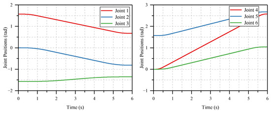
Figure 12.
Actuated joint positions in first group experiment under ORFF.

Figure 13.
Actuated joint velocities in first group experiment under ORFF.
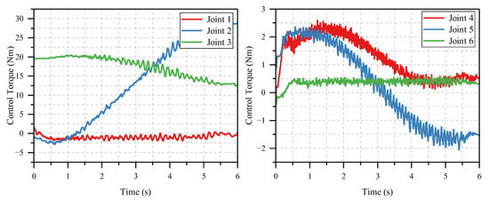
Figure 14.
Control torques in first group experiment under ORFF.
Through the simulation and experimental results, it can be seen that the ORFF achieves better setpoint control performance compared with the FJMFF and CDAEOS. The excellent setpoint control performance indicates that the pose error caused by elastic deformations in all directions is compensated based on the EFJM. Compared with the FJMFF, the execution time of the ORFF is increased as the cost of significant performance improvement. Compared with the CDAEOS, the computational burden of the ORFF is greatly reduced. In addition, the feedforward torques obtained by the ORFF are bounded in all simulations and experiments. Thus, it is indicated that the unstable internal dynamics are transformed into stable ones, which is consistent with the theoretical analysis.
Remark 4.
Although the EFJM is more complicated than the classical FJM, the dynamics model accuracy is improved significantly by using the EFJM. Consequently, the proposed ORFF based on the EFJM can improve the end effector setpoint control precision remarkably.
5. Conclusions
In this paper, a feedforward control method based on the output redefinition of the EFJM is proposed for flexible industrial manipulators. Based on the EFJM, the pose error caused by flexibilities in actuated and nonactuated directions are compensated accurately. By output redefinition, the original nonminimum-phase EFJM is transformed into a minimum-phase system. A recursive feedforward torque computation algorithm is designed to reduce the computational burden. Simulation and experimental results indicate that the proposed method can improve the setpoint control precision significantly compared with traditional feedforward control methods. Future work will focus on extending the feedforward control method to the trajectory tracking control problem and the condition with unknown load.
Author Contributions
Conceptualization, S.X. and Z.W.; methodology, S.X.; software, S.X. and T.S.; validation, S.X.; Writing—original draft, S.X.; writing—review and editing, S.X. and Z.W. All authors have read and agreed to the published version of the manuscript.
Funding
This research was funded by the National Natural Science Foundation of China, grant number U1913206.
Data Availability Statement
The numerical and experimental data sets generated and analyzed during the current study are available from the corresponding author on reasonable request.
Conflicts of Interest
The authors declare no conflict of interest.
References
- Kim, S.H.; Min, B. Joint Compliance Error Compensation for Robot Manipulator Using Body Frame. Int. J Precis. Eng. Manuf. 2020, 21, 1017–1023. [Google Scholar] [CrossRef]
- Tran, D.; Truong, H.; Ahn, K.K. Adaptive Nonsingular Fast Terminal Sliding Mode Control of Robotic Manipulator Based Neural Network Approach. Int. J. Precis. Eng. Manuf. 2021, 22, 417–429. [Google Scholar] [CrossRef]
- Kim, M.J.; Chung, W.K. Disturbance-Observer-Based PD Control of Flexible Joint Robots for Asymptotic Convergence. IEEE Trans. Robot. 2015, 31, 1508–1516. [Google Scholar] [CrossRef]
- Mei, Z.; Chen, L.; Ding, J. Feed-Forward Control of Elastic-Joint Industrial Robot Based on Hybrid Inverse Dynamic Model. Adv. Mech. Eng. 2021, 13, 16878140211038102. [Google Scholar] [CrossRef]
- Cruz Zavala, E.; Nuño, E.; Moreno, J.A. Robust Trajectory-Tracking in Finite-Time for Robot Manipulators Using Nonlinear Proportional-Derivative Control Plus Feed-Forward Compensation. Int. J. Robust Nonlinear Control 2021, 31, 3878–3907. [Google Scholar] [CrossRef]
- Nho, H.C.; Meckl, P. Intelligent Feedforward Control and Payload Estimation for a Two-Link Robotic Manipulator. IEEE/ASME Trans. Mechatron. 2003, 8, 277–283. [Google Scholar] [CrossRef]
- Sun, L.; Zhao, W.; Yin, W.; Sun, N.; Liu, J. Proxy Based Position Control for Flexible Joint Robot with Link Side Energy Feedback. Robot. Auton. Syst. 2019, 121, 103272. [Google Scholar] [CrossRef]
- Spong, M.W. Modeling and Control of Elastic Joint Robots. J. Dyn. Syst. Meas. Control-Trans. ASME 1987, 109, 310–318. [Google Scholar] [CrossRef]
- Consolini, L.; Gerelli, O.; Guarino Lo Bianco, C.; Piazzi, A. Flexible Joints Control: A Minimum-Time Feed-Forward Technique. Mechatronics 2009, 19, 348–356. [Google Scholar] [CrossRef]
- Madsen, E.; Rosenlund, O.S.; Brandt, D.; Zhang, X. Adaptive Feedforward Control of a Collaborative Industrial Robot Manipulator Using a Novel Extension of the Generalized Maxwell-Slip Friction Model. Mech. Mach. Theory 2021, 155, 104109. [Google Scholar] [CrossRef]
- Ohr, J.; Moberg, S.; Wernholt, E.; Hanssen, S.; Pettersson, J.; Persson, S.; Sander-Tavallaey, S. Identification of Flexibility Parameters of 6-Axis Industrial Manipulator Models. In Proceedings of the ISMA2006, Leuven, Belgium, 18–20 September 2006; pp. 3305–3314. [Google Scholar]
- Moberg, S.; Hanssen, S. A DAE Approach to Feedforward Control of Flexible Manipulators. In Proceedings of the IEEE International Conference on Robotics & Automation, Rome, Italy, 10–14 April 2007; pp. 3439–3444. [Google Scholar]
- Moberg, S.; Wernholt, E.; Hanssen, S.; Brog Rdh, T. Modeling and Parameter Estimation of Robot Manipulators Using Extended Flexible Joint Models. J. Dyn. Syst. Meas. Control-Trans. ASME 2014, 136, 031005. [Google Scholar] [CrossRef]
- Bastos, G.; Seifried, R.; Brüls, O. Analysis of Stable Model Inversion Methods for Constrained Underactuated Mechanical Systems. Mech. Mach. Theory 2017, 111, 99–117. [Google Scholar] [CrossRef]
- Moberg, S.; Hanssen, S. Inverse Dynamics of Flexible Manipulators. In Proceedings of the 2009 Conference on Multibody Dynamics, Warsaw, Poland, 29 June–2 July 2009; pp. 1–20. [Google Scholar]
- Seifried, R.; Blajer, W. Analysis of Servo-Constraint Problems for Underactuated Multibody Systems. Mech. Sci. 2013, 4, 113–129. [Google Scholar] [CrossRef]
- Moberg, S. Modeling and Control of Flexible Manipulators; phdMoberg370497; Linköpings University: Linköping, Sweden, 2010. [Google Scholar]
- Luh, J.Y.; Walker, M.W.; Paul, R.P. On-Line Computational Scheme for Mechanical Manipulators. J. Dyn. Syst. Meas. Control-Trans. ASME 1980, 102, 69–76. [Google Scholar] [CrossRef]
- Buondonno, G.; De Luca, A. Efficient Computation of Inverse Dynamics and Feedback Linearization for VSA-Based Robots. IEEE Robot. Autom. Lett. 2016, 1, 908–915. [Google Scholar] [CrossRef]
- Walker, M.W.; Orin, D.E. Efficient Dynamic Computer Simulation of Robotic Mechanisms. J. Dyn. Syst. Meas. Control-Trans. ASME 1982, 104, 205–211. [Google Scholar] [CrossRef]
- Ruderman, M.; Iwasaki, M. Sensorless Torsion Control of Elastic-Joint Robots with Hysteresis and Friction. IEEE Trans. Ind. Electron. 2016, 63, 1889–1899. [Google Scholar] [CrossRef]
- Gaz, C.; Cognetti, M.; Oliva, A.; Robuffo Giordano, P.; De Luca, A. Dynamic Identification of the Franka Emika Panda Robot with Retrieval of Feasible Parameters Using Penalty-Based Optimization. IEEE Robot. Autom. Lett. 2019, 4, 4147–4154. [Google Scholar] [CrossRef]
- Fang, Y.; Hu, J.; Liu, W.; Shao, Q.; Qi, J.; Peng, Y. Smooth and Time-Optimal S-Curve Trajectory Planning for Automated Robots and Machines. Mech. Mach. Theory 2019, 137, 127–153. [Google Scholar] [CrossRef]

Disclaimer/Publisher’s Note: The statements, opinions and data contained in all publications are solely those of the individual author(s) and contributor(s) and not of MDPI and/or the editor(s). MDPI and/or the editor(s) disclaim responsibility for any injury to people or property resulting from any ideas, methods, instructions or products referred to in the content. |
© 2023 by the authors. Licensee MDPI, Basel, Switzerland. This article is an open access article distributed under the terms and conditions of the Creative Commons Attribution (CC BY) license (https://creativecommons.org/licenses/by/4.0/).