Study of Error Flow for Hydraulic System Simulation Models for Construction Machinery Based on the State-Space Approach

Abstract

This study presents an error flow research method for simulation models of hydraulic systems in construction machinery based on the state-space approach, aiming to ensure the reliable application of digital twin models. Initially, a comprehensive analysis of errors in the simulation modeling of hydraulic systems in construction machinery was conducted, highlighting simulation model parameters as the primary error sources. Subsequently, a set of metrics for assessing the accuracy of simulation models was developed. Following this, an error flow analysis method for simulation models of hydraulic systems in construction machinery was explored based on the state space approach, delving into the sources, transmission, and accumulation of errors in the simulation modeling of valve-controlled cylinder systems. The research results unequivocally indicate that the spring stiffness, viscous damping coefficient, and hydraulic cylinder external leakage coefficient are critical parameters affecting the accuracy of valve-controlled cylinder system simulation models. Furthermore, it was observed that the simulation model of the control valve has a significantly greater impact on the errors in the valve-controlled cylinder system simulation model than the hydraulic cylinder model. In conclusion, the reliability of the error flow model was confirmed through simulation experiments, revealing a maximum relative error of only 3.73% between the error flow model and the results of the simulation experiments.

1. Introduction

As simulation, big data, and computer technologies continue to advance, digital twin applications have proliferated in fields such as construction machinery structural optimization, trajectory control, and health monitoring [1,2,3]. In theory, it is feasible to construct digital twin models for construction machinery hydraulic systems. However, limitations in computational accuracy have hindered the full realization of digital twin technology’s potential in hydraulic systems of construction machinery [4]. Digital twin technology is an online simulation method [5,6] in which the simulation model plays a crucial role throughout the entire lifecycle of the digital twin model, serving as a representation of the system in physical, mathematical, or other logical forms [7]. The study of simulation model errors in hydraulic systems of construction machinery holds paramount importance in enhancing model precision, ensuring the robust application of digital twin technology in the domain of hydraulic systems for construction machinery.

Fan et al. [8] employed a truncation error analysis method based on Taylor series expansion to derive error bounds for linear power flow models in electrical systems. Qiu et al. [9] proposed a model parameter error correction approach that relies on sensitivity information and employs a constant value to compensate for model errors. Zhou et al. [10] scrutinized the correlations between parameters such as the outlet oil temperature, oil properties, and environmental temperature with the overall heat transfer coefficient. Through mathematical functions, they explicitly delineated the relationship between each parameter and the overall heat transfer coefficient, unveiling the impact of parameter fluctuations on model errors.

However, it is worth noting that the aforementioned error analysis studies predominantly target individual, standalone systems, whereas the simulation model for hydraulic systems in construction machinery belongs to the category of complex systems. The methods described above are not necessarily applicable to this complex context. In reality, errors in the simulation model parameters for hydraulic systems in construction machinery propagate progressively, akin to the stream of variation observed in the mechanical manufacturing and assembly processes. The concept of “stream of variation” was first introduced by Hu et al. [11] in the context of studying variation propagation and accumulation during the car body assembly process. Subsequently, it found extensive application and research in mechanical manufacturing and assembly processes. Jin et al. [12] introduced control theory into the assembly processes of mechanical products, establishing a state-space model for the stream of variation in mechanical assembly. Currently, the state-space approach has become the primary approach for modeling the stream of variation in mechanical manufacturing and assembly processes [13,14,15]. Notably, Liu C et al. [16] provided a comprehensive exposition of the stream of variation modeling method based on the state-space approach, particularly in the context of molten mold casting processes. The state-space approach allows for concise mathematical expressions of system variations and distinguishes between different types of input variations [17,18]. These characteristics align well with the analysis of parameter errors in the simulation model for hydraulic systems in construction machinery. Hence, the state-space approach serves as a suitable framework for conducting error research in the context of simulation models for construction machinery hydraulic systems. This paper employs this method to investigate errors in the simulation models of construction machinery hydraulic systems. It is important to highlight that in order to differentiate it from the “stream of variation model” commonly used in mechanical manufacturing and assembly processes, the error analysis model for the simulation of hydraulic systems in construction machinery is referred to as the “error flow model”.

In summary, this paper aims to study error propagation in the simulation model of hydraulic systems for construction machinery using the state-space method. The remaining sections of the article are structured as follows: Section 1 analyzes the errors in the simulation modeling of a construction machinery hydraulic system. Section 2 presents a comprehensive evaluation metric for the accuracy of the simulation model. In Section 3, the error flow modeling method based on the state-space approach is explained in detail. Section 4 focuses on the error study of the valve-controlled cylinder system simulation models. Section 5 discusses and analyzes the research findings. Section 6 provides a summary of this paper. Finally, in Section 7, the future prospects of the research are discussed.

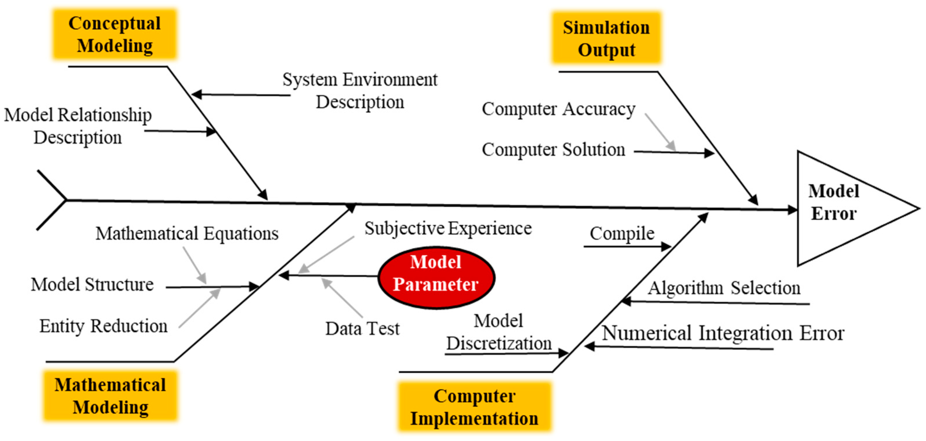
2. Error Analysis in Construction Machinery Simulation Modeling

Simulation modeling involves four stages: conceptual modeling, mathematical modeling, computer implementation, and simulation execution [19]. Model error is a crucial factor affecting the accuracy of simulation models [20]. In general, the error factors in the simulation modeling of hydraulic systems in construction machinery can be categorized as descriptive error, model structure error, model parameter error [21], and computational error. The sources of these errors are illustrated in the fishbone diagram shown in Figure 1. Model structure refers to the mapping relationship between the inputs and outputs of the model. In the process of simulation modeling, it is necessary to mathematically transform and simplify the internal principles and processes of the actual system, which leads to errors known as model structure errors. Even with an accurately determined mathematical relationship in the model structure, the accuracy of the simulation model parameters determines the accuracy of the model outputs. In fact, even if the model structure is highly accurate, the impact of parameter errors on the output results cannot be ignored. Model parameter errors primarily result from limitations related to human experience and experimental testing. Computational errors refer to errors related to the computer in the implementation and simulation output process. This includes the discretization methods within the modeling tools, algorithm selection, errors in the compilation process, errors in the numerical integration and limitations in the accuracy of the computer itself [22,23]. In the process of simulation modeling, both model description and model structure have usually undergone multiple validations by researchers worldwide. Additionally, computational errors are challenging to avoid. Therefore, this study primarily focuses on the influence of simulation model parameter errors on the modeling accuracy of hydraulic systems in construction machinery.

In the process of simulating construction machinery hydraulic systems, models are progressively assembled from multiple subsystems based on fluid dynamics, mechanics, and other relationships. The output from an earlier level determines the input to a later level. Consequently, when errors exist in the parameters at a certain level, these errors continue to propagate and accumulate, thereby affecting the final accuracy of the simulation model for construction machinery hydraulic systems [24]. To ensure the accuracy of the simulation model for construction machinery hydraulic systems, it is imperative to establish a formula for the propagation of parameter errors that describes the errors in the process of simulating construction machinery hydraulic systems. The error propagation in the simulation modeling of construction machinery hydraulic systems is depicted in Figure 2. The simulation model encompasses sequential, selection, parallel, cyclic, and embedded modes. In the sequential mode, the output of the former level model serves as the input for the next level model. In the cyclic mode, a portion of the output from the next level model concurrently becomes part of the input for the former level model. It is worth noting that simulation models for construction machinery hydraulic systems primarily employ the sequential mode. This paper will delve into the propagation and accumulation of model parameter errors in the simulation modeling of construction machinery hydraulic systems, investigate reliable methods for model error analysis and improvement, and provide effective support for the application of digital twin technology in this field.

3. Comprehensive Evaluation Metric for Simulation Model Accuracy

Simulation model error analysis necessitates a well-defined model accuracy assessment metric to serve as an evaluation benchmark. Currently, commonly employed accuracy metrics include Theil’s inequality coefficient [25], mean squared error (MSE) [26], coefficient of determination (R²) [27], as well as disparities in shape, position, and spectral features. These metrics primarily focus on assessing the concordance of simulation model outputs and actual outputs in terms of distance, shape, and spectral characteristics, representing single evaluation metrics. However, for the assessment of accuracy in construction machinery hydraulic system simulation models, it is imperative to consider both frequency domain and time domain characteristics. Single evaluation metrics often fall short of meeting these requirements. Therefore, it is essential to devise a comprehensive accuracy evaluation metric. Furthermore, accuracy assessment of simulation models should adhere to the principles of incorporating at least one dimensionless statistical parameter, an error statistical dataset, and a graphical visualization technique [28]. The radar chart is a frequently employed comprehensive performance assessment method, providing an intuitive representation of the accuracy status of the subject under evaluation [29,30]. Hence, a comprehensive evaluation metric based on the radar chart method and accuracy assessment principles is intended to be devised to meet the requirements of error analysis in simulation models of construction machinery hydraulic systems. This metric will encompass the assessment of disparities in the coefficient of determination (R²), shape, position, and spectral characteristics, employing radar charts to evaluate the accuracy of construction machinery hydraulic system simulation models.

The coefficient of determination (R²) is a typical dimensionless statistical parameter that depicts the degree of collinearity between simulation data and reference data. Here is the formula for its computation:

$$R^2={\left[\frac{{{\displaystyle \sum }}_{i=1}^M(x_s(i)-\overline{x_s})(x_r(i)-\overline{x_r})}{\sqrt{{{\displaystyle \sum }}_{i=1}^M{(x_s(i)-\overline{x_s})}^2}\sqrt{{{\displaystyle \sum }}_{i=1}^M{(x_r(i)-\overline{x_r})}^2}}\right]}^2$$

(1)

The output from the hydraulic system of construction machinery is dynamic, requiring decomposition into trend components and random components. The evaluation of trend component data accuracy entails the examination of disparities in both shape and positional features. The equations for these are as follows:

$$e_f=\frac{1}{T}\sqrt{{\displaystyle \sum }_{i=1}^T{\left[z\left(i\right)\right]}^2}$$

(2)

$$e_p=\frac{1}{T}\sqrt{{\displaystyle \sum }_{i=1}^T{\left[z\left(i\right)-\overline{z}\right]}^2}$$

(3)

where x_s(i) and x_r(i) represent simulated data and reference data, respectively, and i = 1, 2, 3,..., T, with T denoting the sample time duration. $\overline{x_s}=\frac{{\displaystyle \sum _{i=1}^T{x}_s\left(i\right)}}{T}$, $\overline{x_r}=\frac{{\displaystyle \sum _{i=1}^T{x}_r\left(i\right)}}{T}$ and $z\left(i\right)=x_s\left(i\right)-x_r\left(i\right)$, $\overline{z}=\frac{{\displaystyle \sum _{i=1}^{T}z\left(i\right)}}{T}$.

In addition, the random data components are transformed into the frequency domain using the windowed spectral analysis method to characterize spectral feature disparities:

$$q_s=\frac{m}{M}$$

(4)

where M represents the number of points at which random components are transformed into the frequency domain, and m denotes the number of points validated through compatibility testing.

The variables e_f and e_p are part of the error statistical data within the accuracy evaluation metric, and their values fall within the range of [0, +∞). They require normalization through Equations (5) and (6):

$$q_{fs}=1-\frac{e_f}{{\overline{e_f}}_{mxa}}$$

(5)

$$q_{ps}=1-\frac{e_p}{{\overline{e_p}}_{mxa}}$$

(6)

where ${\overline{e_f}}_{mxa}$ represents the maximum value of statistical data among various models $\overline{e_f}=\frac{1}{T}\sqrt{T{\left(\max \left(z\left(i\right)\right)\right)}^2}$, and ${\overline{e_p}}_{mxa}$ represents the maximum value of statistical data among various models $\frac{1}{T}\sqrt{T{\left(\max \left(z\left(i\right)-\overline{z}\right)\right)}^2}$.

Represent the accuracy evaluation metric vector as $Q_d=[q_{fs} q_{ps} q_s R^2]$ and conduct a visual and comprehensive assessment of the individual evaluation metrics within the vector using a radar chart. The specific steps are as follows:

(a)

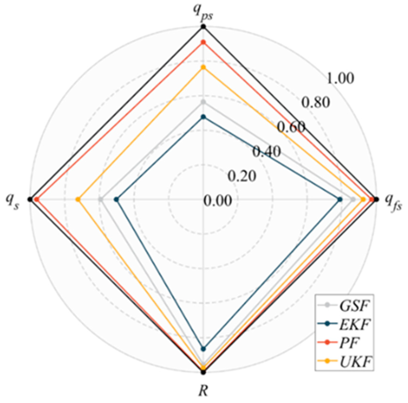
Generate radar charts based on the metrics.

(b)

Calculate the area $S_{index}$ enclosed by different metrics.

(c)

Calculate the area $S_T$ enclosed when all metrics are set to 1.

(d)

Compute the comprehensive evaluation metric $l=\sqrt{\frac{S_{index}}{S_T}}$ based on the areas $S_{index}$ and $S_T$. It falls within the range of [0, 1], where a higher value of “l” indicates greater model accuracy, with “1 − l” representing the model’s error characterization.

Taking the example of a nonlinear and non-Gaussian dynamic output model from reference [31], the accuracies of four different filters are evaluated using the comprehensive evaluation metric “l”. After computation, the results for the four models’ TRUE, GSF, EKF, PF and UKF are as shown in

Table 1. Accuracy evaluation metrics for each model.

Model	qfs	qps	qs	R2
GSF	0.865	0.564	0.593	0.955
EKF	0.789	0.477	0.502	0.865
PF	0.972	0.909	0.962	0.995
UKF	0.924	0.765	0.723	0.974

. Here, TRUE, GSF, EKF, PF, and UKF denote the actual results, Gaussian Sum Filter, Extended Kalman Filter, Particle Filter, and Unscented Kalman Filter prediction outcomes, respectively.

Based on the results in Table 1, radar charts, as illustrated in Figure 3, were generated, with model accuracy results as follows: $l_{GSF}$ = 0.553, $l_{EKF}$ = 0.433, $l_{PF}$ = 0.921 and $l_{UKF}$ = 0.716. The models’ accuracy rankings, from highest to lowest, are PF, UKF, GSF, and EKF, consistent with the findings reported in reference [31]. The comprehensive evaluation metric “l” aligns with the principles of accuracy assessment in simulation models, allowing for a reasonable and accurate evaluation of the model accuracy. It can be effectively applied to error analysis in hydraulic system simulation models for construction machinery.

4. Error Flow Modeling Based on the State-Space Approach

Using a comprehensive accuracy evaluation metric as the assessment criterion, the error flow modeling method for a hydraulic system simulation model for construction machinery, based on the state-space approach, is depicted as shown in Figure 4. The specific steps are outlined as follows:

(1)

Analysis and Characterization of Model Parameter Errors

In the process of hydraulic system modeling for construction machinery, the error flow manifests the relationship between parameter errors and the simulation model errors. The accuracy of the model is largely contingent upon the adopted simulation parameters. However, the process of acquiring these parameters is intricate and susceptible to various influences, inevitably leading to the emergence of parameter errors, which further impacts the accuracy and reliability of the model. In the process of modeling hydraulic systems in construction machinery, simulation parameters are mainly determined through experience and experimental testing. However, often there are situations where parameters are unknown or cannot be measured accurately. This deviation from the target parameter values affects the accuracy of the simulation model.

Measurement errors can be categorized into three types: systematic errors, random errors, and gross errors [32]. Systematic errors result from fixed factors and, when experiments are conducted under the same conditions multiple times, the error values remain constant. Random errors, on the other hand, stem from uncontrollable factors, leading to uncertainty in error values when conducting multiple experiments under similar conditions. The influence of random errors can be mitigated by conducting multiple experiments and employing the method of averaging. Both of these error types are inevitable. Gross errors, however, are caused by occasional and exceptional factors and should be excluded from a series of experimental measurement data. Errors that arise due to human experience are rooted in a lack of knowledge or incomplete information. These errors exhibit randomness and vary with the degree of personal understanding.

Through the aforementioned analysis, the causes of parameter errors in construction machinery hydraulic system modeling have been clarified. In the state-space approach, assuming the n_th system contains $\lambda$ key parameters, the parameter vector of the n_th system can be defined as follows:

$$\phi \left(n\right)=\left({\epsilon }_1\left(n\right),{\epsilon }_2\left(n\right),\cdots ,{\epsilon }_{\mathsf{\lambda }}\left(n\right)\right)$$

(7)

The parameter error vector $\Delta \phi \left(n\right)$ for the n_th system is denoted as follows:

$$\Delta \phi \left(n\right)=\left(\Delta {\epsilon }_1\left(n\right),\Delta {\epsilon }_2\left(n\right),\cdots ,\Delta {\epsilon }_{\mathsf{\lambda }}\left(n\right)\right)$$

(8)

where n represents the number of model subsystems, $\lambda$ represents the number of subsystem model parameters, and ${\epsilon }_{\lambda }\left(n\right)$ represents the error of the ${\lambda }_{th}$ parameter of the n_th subsystem relative to the target parameter.

(2)

Obtaining Reference Parameters

The parameter errors discussed are in relation to the target parameters of the simulation model. In engineering research, acquiring simulation model parameters with absolute accuracy and establishing a simulation model of utmost accuracy pose significant challenges and are often unfeasible. Hence, the model parameters that yield the highest accuracy evaluation metric “l” for the simulation model will be selected, and they will be designated as the reference parameters for the simulation model in lieu of the target parameters. Additionally, the model parameter error $\Delta \phi \left(n\right)$ is defined as the disparity between the model parameters $\phi \left(n\right)$ and the reference parameters ${\phi }^t\left(n\right)$. The process for acquiring reference parameters for the simulation model is as follows:

(a)

Establish the simulation model for the hydraulic system in construction machinery.

(b)

Obtain experimental data as reference data for the simulation model and refine it through multiple experiments to reduce gross errors and random errors.

(c)

Compare the output results of the simulation model with the reference data and assess the model’s accuracy using evaluation metric “l”.

(d)

As the optimization objective, seek to maximize evaluation metric “l” and employ optimization algorithms such as particle swarm optimization (PSO) [33] to solve for the reference parameters.

(3)

Model Expected Accuracy and Model Error Change Rate

The model accuracy result $l^t(n)$ of the model established based on the reference parameter ${\phi }^t\left(n\right)$ represents the expected accuracy of the model. On the other hand, to depict the variation in model accuracy, a function for the model error change rate is defined. The error change rate function $s\left(n\right)$ for the n_th subsystem model under model parameters $\phi \left(n\right)$ is represented as follows:

$$s\left(n\right)=\frac{l\left(n\right)}{l\left(n-1\right)}$$

(9)

where, $l\left(n\right)$ and $l\left(n-1\right)$ represent the accuracy of the n_th and (n − 1)_th subsystem models under different model parameters. Based on the definition of the model error change rate, the accuracy of the n_th subsystem model can be expressed as

$$l\left(n\right)=s\left(n\right)l\left(n-1\right)$$

(10)

(4)

Relationship between Model Parameters and Error Change Rate

As in Equation (10), it is evident that the model error change rate of the n_th subsystem directly influences the accuracy of that subsystem model. The error change rate is associated with the subsystem model parameters, and deviations of these parameters from the reference values can induce fluctuations in the model error change rate, subsequently affecting model accuracy. The relationship between these two is defined as

$$s\left(n\right)=f\left(\phi \left(n\right)\right)$$

(11)

To represent the relationship between model parameters and the model error change rate, it is essential to conduct simulation experiments based on experimental data and simulation models to calculate the model error change rate under various model parameter samples. A central composite experimental design (CCD) method [34] is employed to design simulation experiment samples. Utilizing these experimental samples, a function relationship between the parameters and model error change rate is established using the response surface method (RSM) [35,36].

(5)

Mathematical Formulation of Error Flow

As in Equation (10), the model error induced by simulation parameter errors during the modeling process can be expressed as

$$\mathsf{\Delta }l\left(n\right)=s\left(n\right)l\left(n-1\right)-s^t\left(n\right)l^t\left(n-1\right)$$

(12)

where $s^t\left(n\right)$ represents the error change rate of the n_th subsystem when parameters are set to their reference values, while $l^t\left(n-1\right)$ represents the expected accuracy of the (n − 1)_th subsystem when parameters are set to their reference values.

Based on Equations (11) and (12), it can be deduced that the model error induced by simulation parameter errors is as follows:

$$\mathsf{\Delta }l\left(n\right)=f\left(\phi \left(n\right)\right)l\left(n-1\right)-f\left({\phi }^t\left(n\right)\right)l^t\left(n-1\right)$$

(13)

Equations (14) and (15) are obtained by expanding Equation (13) around the reference parameters using the Taylor series,

$$\mathsf{\Delta }l\left(n\right)=f\left({\phi }^t\left(n\right)\right)\mathsf{\Delta }l\left(n-1\right)+f^{\prime }\left({\phi }^t\left(n\right)\right)l^t\left(n-1\right)\mathsf{\Delta }\phi \left(n\right)+h\left(\mathsf{\Delta }\phi \left(n\right)\right)$$

(14)

$$h\left(\mathsf{\Delta }\phi \left(n\right)\right)=r\left(\mathsf{\Delta }\phi \left(n\right)\right)\left(l^t\left(n-1\right)+\mathsf{\Delta }l\left(n-1\right)\right)+f^{\prime }\left({\phi }_{\mathrm{t}}\left(n\right)\right)\mathsf{\Delta }\phi \left(n\right)$$

(15)

where $r\left(\mathsf{\Delta }\phi \left(n\right)\right)$ represents the higher-order residual term of $\mathsf{\Delta }\phi \left(n\right)$, while $h\left(\mathsf{\Delta }\phi \left(n\right)\right)$ denotes the interference of other random factors with negligible magnitudes.

Further simplification yields the error flow expression in the modeling process of a construction machinery hydraulic system simulation model:

$$\mathsf{\Delta }l\left(n\right)=f\left({\phi }^t\left(n\right)\right)\mathsf{\Delta }l\left(n-1\right)+f^{\prime }\left({\phi }^t\left(n\right)\right)l^t\left(n-1\right)\mathsf{\Delta }\phi \left(n\right)$$

(16)

5. Case Study: Valve-Controlled Cylinder System

5.1. Error Sources of the Valve-Controlled Cylinder System Model

The valve-controlled cylinder system is a typical subject of study in hydraulics. Rahmat et al. [37] conducted research on the control system of the electrohydraulic actuator system. Andrzej et al. [38] investigated the control of the electrohydraulic linear actuator. Zhang et al. [39] carried out modeling and model parameter sensitivity analysis on the valve-controlled helical hydraulic rotary actuator system. However, there is currently no reported research on the error flow analysis in the modeling process of the valve-controlled cylinder system. Therefore, this paper, taking the simulation model of the valve-controlled cylinder system as an example, conducts an error analysis on its simulation modeling process. The valve-controlled cylinder system primarily comprises two subsystems, i.e., the control valve and the hydraulic cylinder, as shown in Figure 5.

The mathematical model of the control valve is represented by the spool dynamics equation and the inlet/outlet flow equations of the control valve [40,41,42]:

$$P_{pilot}{A}_v-F_0=m_v\frac{d^2{x}_v}{d{t}^2}+B_v\frac{d{x}_v}{dt}+K_v{x}_v$$

(17)

$$q_1=\left\{\begin{array}{l}{C}_q{f}_A\sqrt{2(p_p-p_A)/\rho }\hspace{1em}{x}_v>0\\ 0\hspace{1em}\hspace{1em}\hspace{1em}\hspace{1em}\hspace{1em}\hspace{1em}\hspace{1em} x_v=0\\ C_q{f}_A\sqrt{2(p_A-p_T)/\rho }\hspace{1em}{x}_v<0\end{array}\right.$$

(18)

$$q_2=\left\{\begin{array}{l}{C}_q{f}_A\sqrt{2(p_B-p_T)/\rho }\hspace{1em}{x}_v>0\\ 0\hspace{1em}\hspace{1em}\hspace{1em}\hspace{1em}\hspace{1em}\hspace{1em}\hspace{1em} x_v=0\\ C_q{f}_A\sqrt{2(p_p-p_B)/\rho }\hspace{1em}{x}_v<0\end{array}\right.$$

(19)

where P_pilot is the pilot pressure, A_v is the valve spool cross-sectional area, and F₀ is the external force applied to the control valve. The valve spool is primarily subjected to static pressures, such as spring preload, and the impacts of transient fluid dynamics and frictional forces on the control valve were ignored. m_v is the mass of the valve spool, B_v is the damping coefficient, K_v is the spring stiffness, x_v is the displacement of the valve spool, C_q is the flow rate coefficient, f_A is the overflow area, p_p is the main pump outlet pressure, p_T is the tank pressure, p_A is the cylinder large cavity pressure, and p_B is the cylinder small cavity pressure.

The mathematical model of the hydraulic cylinder includes the flow rate equation and the force balance equation:

$$\left\{\begin{array}{l}{q}_1=A_A\frac{dy}{dt}+C_i\left(p_A-p_B\right)+C_e{p}_A+\frac{V_{\mathrm{A}}}{{\beta }_e}\frac{d{p}_A}{dt}\hfill \\ \begin{array}{l}{V}_A=V_{A0}+A_{A}y\\ V_{A0}=V_{Ad}+A_A{L}_0\end{array}\hfill \end{array}\right.$$

(20)

$$\left\{\begin{array}{l}{q}_2=A_B\frac{dy}{dt}+C_i\left(p_A-p_B\right)-C_e{p}_B-\frac{V_B}{{\beta }_e}\frac{d{p}_B}{dt}\hfill \\ \begin{array}{l}{V}_B=V_{B0}-A_{B}y\\ V_{B0}=V_{Bd}+A_B\left(L-L_0\right)\end{array}\hfill \end{array}\right.$$

(21)

$$A_A{p}_A-A_B{p}_B=M\frac{d{y}^2}{dt}+B_p\frac{dy}{dt}+Ky+F_f+F_l$$

(22)

where A_A and A_B are the piston areas of cylinder’s large and small cavities, y is the displacement of the cylinder, C_i and C_e are the cylinder’s internal and external leakage coefficients, respectively, β_e is the equivalent bulk elastic modulus of hydraulic oil, V₀₁ and V₀₂ are the initial volumes of large and small cavities, and P_A and P_B are the pressures in the cylinder’s large and small cavities. V_Ad and V_Bd are the dead zone volumes of the large and small cavities of the cylinder, respectively, L is the maximum stroke of the cylinder, and L₀ is the initial position of the cylinder. M is the total mass of the cylinder, B_p is the damping coefficient of the cylinder, K is the load stiffness, F_f is the coulomb friction, and F_l is the load force. In this paper, the minor friction force F_f relative to the load force F_l is ignored in a valve-controlled cylinder system.

According to the working principle of the valve-controlled cylinder system, the primary parameters in the simulation model include the control valve model parameters, namely, F₀, K_v, B_v and C_q, as well as the cylinder model parameters, C_i, C_e, β_e and B_p. The parameter vectors for the two subsystems and their respective error vectors are defined as follows:

$$\phi \left(1\right)=({\epsilon }_1\left(1\right),{\epsilon }_2\left(1\right),{\epsilon }_3\left(1\right),{\epsilon }_4\left(1\right))$$

(23)

$$\Delta \phi \left(1\right)=(\Delta {\epsilon }_1\left(1\right),\Delta {\epsilon }_2\left(1\right),\Delta {\epsilon }_3\left(1\right),\Delta {\epsilon }_4\left(1\right))$$

(24)

$$\phi \left(2\right)=({\epsilon }_1\left(2\right),{\epsilon }_2\left(2\right),{\epsilon }_3\left(2\right),{\epsilon }_4\left(2\right))$$

(25)

$$\Delta \phi \left(2\right)=(\Delta {\epsilon }_1\left(2\right),\Delta {\epsilon }_2\left(2\right),\Delta {\epsilon }_3\left(2\right),\Delta {\epsilon }_4\left(2\right))$$

(26)

where ${\epsilon }_1\left(1\right),{\epsilon }_2\left(1\right),{\epsilon }_3\left(1\right)$ and ${\epsilon }_4\left(1\right)$ represent the control valve model parameters F₀, K_v, B_v and C_q, respectively. $∆{\epsilon }_1\left(1\right),{∆\epsilon }_2\left(1\right),{∆\epsilon }_3\left(1\right)$ and ${∆\epsilon }_4\left(1\right)$ represent the error of parameters F₀, K_v, B_v and C_q, respectively. ${\epsilon }_1\left(2\right),{\epsilon }_2\left(2\right),{\epsilon }_3\left(2\right)$ and ${\epsilon }_4\left(2\right)$ represent the cylinder model parameters C_i, C_e, β_e and B_p, respectively. $∆{\epsilon }_1\left(2\right),{∆\epsilon }_2\left(2\right),{∆\epsilon }_3\left(2\right)$ and ${∆\epsilon }_4\left(2\right)$ represent the errors of parameters C_i, C_e, β_e and B_p, respectively.

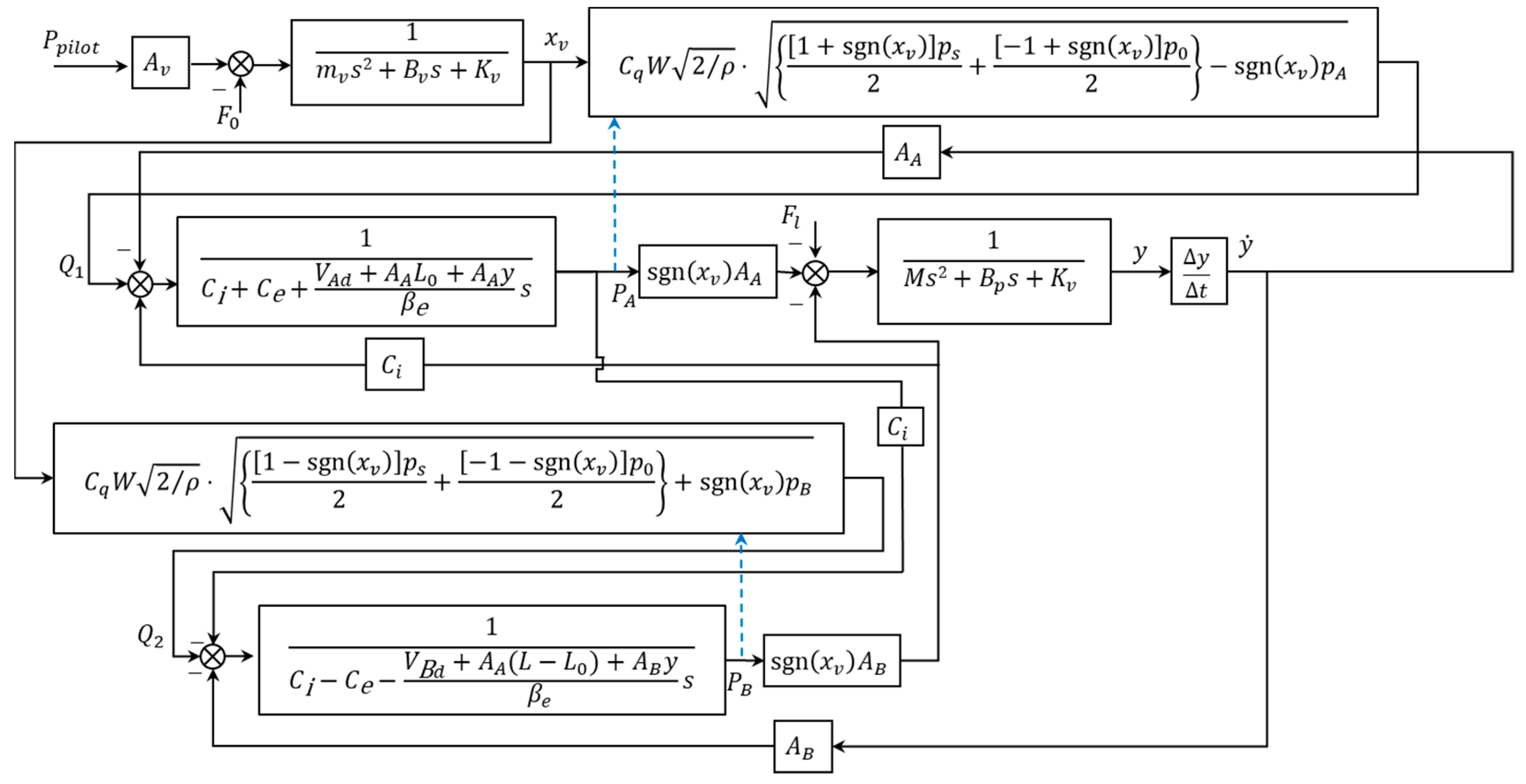
5.2. Error Flow Modeling of the Valve-Controlled Cylinder System

The process of modeling the error flow in the valve-controlled cylinder system model is illustrated in Figure 6. Based on the state-space approach, the mathematical relationship expressing the impact of parameter errors on model errors can be established by constructing functional connections among the control valve parameter vector, hydraulic cylinder parameter vector, and the model error change rates.

First, the simulation model of the valve-controlled cylinder system is established based on Equations (17)–(22), and the results are depicted in Figure 7. Additionally, the reference parameters for the control valve and hydraulic cylinder models were determined using the particle swarm optimization (PSO) algorithm, denoted as ${\mathsf{\phi }}^t\left(1\right)=\left(297.374, 130.285, 299.386, 0.695\right)$ and ${\mathsf{\phi }}^t\left(2\right)=(387.808, 297.641, 958.414, 825.140)$, respectively, utilizing experimental data as a reference.

Second, the central composite design (CCD) method is utilized for experimental design in simulation trials. Central composite design (CCD) is a method employed within the context of the response surface method (RSM), with the objective of systematically exploring and optimizing the influence of multiple factors on the response of a given system. This involves strategically selecting experimental points, including those at the center, boundaries, and additional axial points within the designated design space, to facilitate the construction of a polynomial response surface model. The experimental factors and levels for the control valve model and hydraulic cylinder model are presented in

Table 2. Accuracy evaluation metrics for each model.

Levels	${\mathit{\epsilon }}_1\left(1\right)$/(N)	${\mathit{\epsilon }}_1\left(2\right)$/(N/m)	${\mathit{\epsilon }}_3\left(1\right)$/(Nm/s)	${\mathit{\epsilon }}_4\left(1\right)$
−alpha	257.324	105.285	259.386	0.495
low	277.324	120.285	279.386	0.595
0	297.324	130.285	299.386	0.695
high	317.324	150.285	319.386	0.795
+alpha	337.324	165.285	339.386	0.895

and

Table 3. Experimental factors and levels of the hydraulic cylinder model.

Levels	${\mathit{\epsilon }}_1\left(2\right)$/(mm3/MPa/s)	${\mathit{\epsilon }}_2\left(2\right)$/(mm3/MPa/s)	${\mathit{\epsilon }}_3\left(2\right)$/(MPa)	${\mathit{\epsilon }}_4\left(2\right)$/(N·s/m)
−alpha	2.878	2.351	758.414	78,514
low	3.378	2.726	858.414	80,514
0	3.878	2.976	958.414	82,514
high	4.378	3.476	1058.414	84,514
+alpha	4.878	3.851	1158.414	86,514

, respectively. In the table, alpha represents the axial points in the central composite design (CCD) method.

Simulation models for the control valve and hydraulic cylinder were established based on the samples from Table 2 and Table 3, respectively. The error change rates of the simulation models for the control valve and hydraulic cylinder were computed using Equation (9), model samples, and reference experimental data. The results are presented in

Table 4. Error change rate samples for the control valve model.

Serial Number	${\mathit{\epsilon }}_1\left(1\right)$/(N)	${\mathit{\epsilon }}_1\left(2\right)$/(N/m)	${\mathit{\epsilon }}_3\left(1\right)$/(Nm/s)	${\mathit{\epsilon }}_4\left(1\right)$	Error Change Rates
1	297.324	130.285	299.386	0.895	0.901534
2	317.324	150.285	319.386	0.795	0.836035
3	317.324	150.285	319.386	0.595	0.836035
4	297.324	90.285	299.386	0.695	0.0592399
5	297.324	130.285	299.386	0.695	0.901534
6	297.324	130.285	299.386	0.495	0.901534
7	317.324	110.285	319.386	0.795	0.495151
8	297.324	170.285	299.386	0.695	0.614629
9	317.324	110.285	319.386	0.595	0.495151
10	317.324	150.285	279.386	0.595	0.816725
11	277.324	110.285	279.386	0.595	0.549803
12	297.324	130.285	299.386	0.695	0.901534
13	277.324	150.285	279.386	0.595	0.816725
14	317.324	110.285	279.386	0.795	0.549803
15	277.324	110.285	319.386	0.595	0.495151
16	277.324	150.285	319.386	0.795	0.836035
17	277.324	150.285	279.386	0.795	0.816725
18	277.324	110.285	319.386	0.795	0.495151
19	297.324	130.285	339.386	0.695	0.867413
20	277.324	150.285	319.386	0.595	0.836035
21	317.324	150.285	279.386	0.795	0.816725
22	297.324	130.285	259.386	0.695	0.929980

and

Table 5. Error change rate samples for the cylinder model.

Serial Number	${\mathit{\epsilon }}_1\left(2\right)$/(mm3/MPa/s)	${\mathit{\epsilon }}_2\left(2\right)$/(mm3/MPa/s)	${\mathit{\epsilon }}_3\left(2\right)$/(MPa)	${\mathit{\epsilon }}_4\left(2\right)$/(N·s/m)	Error Change Rates
1	437.808	347.641	1058.41	80,514	0.985792
2	387.808	297.641	958.412	82,514	0.985787
3	387.808	297.641	758.416	82,514	0.887663
4	387.808	297.641	958.412	82,514	0.887662
5	337.808	347.641	1058.41	84,514	0.996764
6	387.808	197.641	958.412	82,514	0.996764
7	437.808	347.641	1058.41	84,514	0.985792
8	337.808	247.641	1058.41	84,514	0.996768
9	287.808	297.641	958.412	82,514	0.985789
10	437.808	247.641	858.414	80,514	0.887665
11	437.808	247.641	1058.41	84,514	0.887663
12	337.808	247.641	858.414	84,514	0.985789
13	337.808	247.641	1058.41	80,514	0.996764
14	437.808	247.641	1058.41	80,514	0.985794
15	387.808	297.641	958.412	86,514	0.99677
16	487.808	297.641	958.412	82,514	0.990749
17	437.808	247.641	858.414	84,514	0.887663
18	337.808	347.641	1058.41	80,514	0.985794
19	337.808	247.641	858.414	80,514	0.996768
20	437.808	347.641	858.414	84,514	0.985794
21	387.808	297.641	958.412	82,514	0.99677
22	387.808	397.641	958.412	82,514	0.887663
23	337.808	347.641	858.414	84,514	0.887663
24	387.808	297.641	958.412	82,514	0.773039
25	437.808	347.641	858.414	80,514	0.996768
26	387.808	297.641	1158.41	82,514	0.985796
27	387.808	297.641	958.412	78,514	0.887663
28	337.808	347.641	858.414	80,514	0.985789

.

Finally, mathematical expressions for the error change rates of the control valve and hydraulic cylinder models are derived through the use of the response surface method (RSM), utilizing the experimental samples in Table 4 and Table 5. The functional relationship between the control valve model and hydraulic cylinder model error change rate and the parameter vectors $\phi \left(1\right)$ and $\phi \left(2\right)$ are shown as Equations (27) and (28). After computation, it was determined that the RSM of the control valve simulation exhibited high determination coefficients, with R², Adjusted R², and Predicted R² values of 0.975, 0.969, and 0.922, respectively. These significant values indicate a robust fit of the control valve model’s RSM. Similarly, the RSMs of the hydraulic cylinder simulation model demonstrated outstanding determination coefficients, with R², Adjusted R², and Predicted R² values of 0.999, 0.998, and 0.978, respectively. This also signifies an excellent level of fit for the hydraulic cylinder model’s RSM.

$$\begin{array}{l}s(1)=f(\phi (1))=-5.588+0.101K_v-6.578\times {10}^{-3}{B}_v\\ +1.222C_q+5.600\times {10}^{-6}{K}_v{B}_v-4.120\times {10}^{-4}{K}_v{}^2\\ -0.872C_q{}^2\end{array}$$

(27)

$$\begin{array}{l}s(2)=f(\phi (2))=-5.299+1.903C_e-3.100\times {10}^{-5}{\beta }_e\\ +1.540\times {10}^{-4}{B}_p-4.600\times {10}^{-5}{C}_e{B}_p-5.812\times {10}^{-3}{C}_e{}^2\\ +1.669\times {10}^{-8}{\beta }_e{}^2-9.377\times {10}^{-10}{B}_p{}^2+2.785\times {10}^{-10}{C}_e{B}_p{}^2\end{array}$$

(28)

The error flow model for the valve-controlled cylinder system simulation can be derived by substituting the error change rate functions of the control valve and hydraulic cylinder simulation models into the error flow expression (Equation (16)):

$$\begin{array}{l}\Delta l(1)=f({\phi }^t(1))\Delta l(0)+l^t(0)f^{\prime }({\phi }^t(1))\Delta \phi (1)\\ =0+1\times f^{\prime }({\phi }^t(1))\Delta \phi (1)=f^{\prime }({\phi }^t(1))\Delta \phi (1)\\ =[0, -6.680\times {10}^{-3}, -5.849\times {10}^{-3}, 2.680\times {10}^{-6}]{[\Delta F_0 \Delta K_v \Delta B_v \Delta C_q]}^T\end{array}$$

(29)

$$\begin{array}{l}\Delta l(2)=f({\phi }^t(2))\Delta l(1)+l^t(1)f^{\prime }({\phi }^t(2))\Delta \phi (2)\\ =l^t(2)f^{\prime }({\phi }^t(1))\Delta \phi (1)+l^t(1)f^{\prime }({\phi }^t(2))\Delta \phi (2)\\ =0.9955\times [0,-6.680\times {10}^{-3},-5.849\times {10}^{-3}, 2.680\times {10}^{-6}]{[\Delta F_0 \Delta K_v \Delta B_v \Delta C_q]}^T\\ +0.9527\times [0, 0.032, 9.915\times {10}^{-7}, -8.892\times {10}^{-6}]{[\Delta C_i \Delta C_e\Delta {\beta }_e \Delta B_p]}^T\end{array}$$

(30)

Equations (29) and (30) represent the error flow models for the control valve and the valve-controlled cylinder system, respectively.

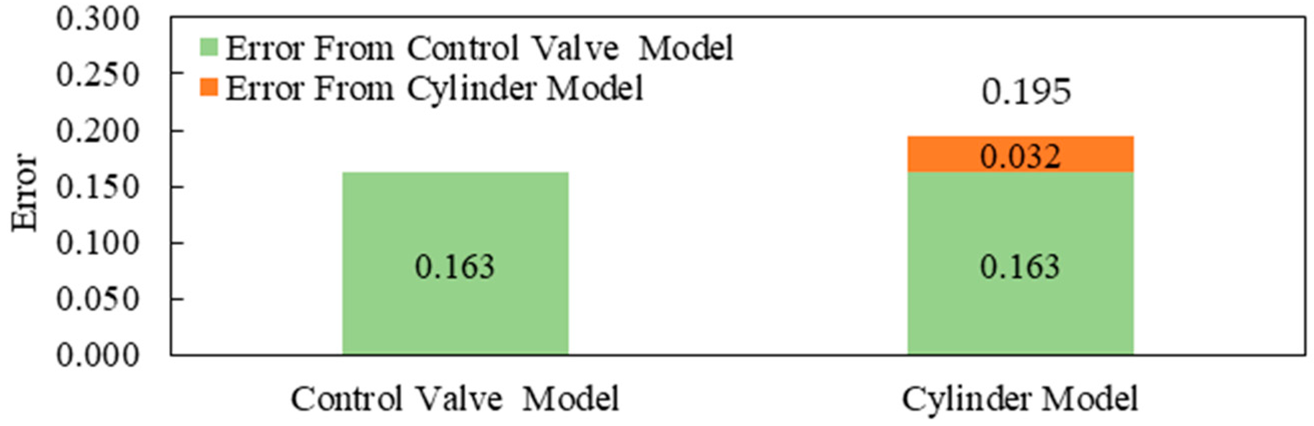
6. Results and Discussion

Using the error flow model, variations in the accuracy of the simulation model for the valve-controlled cylinder system can be assessed by calculating the parameter error vectors. For instance, when the subsystem parameter error vectors are $\Delta \phi (1)={\left[20,-10,-20,0.1\right]}^T$ and $\Delta \phi (2)={\left[0.5,0.5,100,-2000\right]}^T$, the errors in various subsystem models within the valve-controlled cylinder system simulation model are illustrated in Figure 8. The error in the control valve model is 0.163, while the error in the valve-controlled cylinder system model is 0.195. The contributions of the errors in the control valve and hydraulic cylinder models to the error in the valve-controlled cylinder system model are 0.163 and 0.032, respectively. Thus, it is essential to focus on the parameters of the control valve model to ensure its accuracy.

The error flow model elucidates the pathways for the transmission of errors within various subsystem models. The coefficient of the model reflects the influence of parameter errors on the accuracy of the model for the valve-controlled cylinder system. In the valve-controlled cylinder system, the parameters that have the most significant impact on the accuracy of the model are the spring stiffness ${\epsilon }_2\left(1\right)$, viscous damping coefficient ${\epsilon }_3\left(1\right)$, and hydraulic cylinder external leakage coefficient ${\epsilon }_2\left(2\right)$. Therefore, in the process of modeling the valve-controlled cylinder system, efforts should be made to minimize the errors between these three parameters and their reference values. As indicated by Equations (29) and (30), the external force ${\epsilon }_1\left(1\right)$ applied to the control valve and the internal leakage coefficient of the hydraulic cylinder ${\epsilon }_1\left(2\right)$ do not affect the accuracy of the valve-controlled cylinder system model. The spring stiffness ${\epsilon }_2\left(1\right)$, viscous damping coefficient ${\epsilon }_3\left(1\right)$, and hydraulic cylinder damping coefficient ${\epsilon }_4\left(2\right)$ exhibit a negative correlation with the error in the valve-controlled cylinder system model.

The error flow model was employed to calculate the errors in the model corresponding to four sets of parameter samples in

Table 6. Parameter samples of the valve-controlled cylinder system model.

Samples	The Control Valve Model Parameters				The Hydraulic Cylinder Model Parameters
	${\mathit{\epsilon }}_1\left(1\right)$	${\mathit{\epsilon }}_2\left(1\right)$	${\mathit{\epsilon }}_3\left(1\right)$	${\mathit{\epsilon }}_4\left(1\right)$	${\mathit{\epsilon }}_1\left(2\right)$	${\mathit{\epsilon }}_2\left(2\right)$	${\mathit{\epsilon }}_3\left(2\right)$	${\mathit{\epsilon }}_4\left(2\right)$
1	314.884	118.076	318.576	0.618	3.777	2.572	942.981	83,180.112
2	312.362	119.322	296.941	0.654	3.905	2.812	967.988	81,226.530
3	300.806	127.713	295.735	0.697	4.006	2.782	1055.024	81,198.484
4	285.634	122.729	303.182	0.612	3.670	3.333	918.705	80,644.403

. These errors were then compared to the results of the simulation model. The results are presented in

Table 7. Error results of the valve-controlled cylinder system model.

Samples	The Control Valve Model Parameter			The Hydraulic Cylinder Model Parameter
	Results of Stream of Variation Model	Results of Simulation Model	Relative Error	Results of Stream of Variation Model	Results of Simulation Model	Relative Error
1	10.55%	10.39%	1.54%	11.67%	11.43%	2.10%
2	8.32%	8.56%	2.72%	8.89%	8.69%	2.40%
3	1.77%	1.84%	3.68%	2.47%	2.55%	2.97%
4	6.06%	6.29%	3.73%	6.95%	6.76%	2.86%

, which shows that the relative errors between the error flow model and the simulation results are relatively small, with a maximum value of only 3.73%. This indicates a high level of accuracy in the error flow model’s calculations. Among these four sample sets, smaller errors in the spring stiffness ${\epsilon }_2\left(1\right)$ and hydraulic cylinder external leakage coefficient ${\epsilon }_2\left(2\right)$ correspond to smaller model errors, thereby validating the significant influence of these two parameters on the model accuracy.

Simulation engineers can efficiently simulate and compute errors within the simulation models of construction machinery hydraulic systems using error flow models. This approach enables the analysis of error propagation pathways and accumulation processes, offering valuable guidance for simulation parameter control and optimization. The improvement and optimization of the accuracy of construction machinery hydraulic system models through error flow models can significantly enhance the computational accuracy of digital twin models. This, in turn, facilitates the possibility of detecting and tracking the accuracy of digital twin models, thereby providing robust support for the widespread adoption and application of digital twin technology in the realm of construction machinery hydraulic systems.

7. Conclusions

This paper addresses the issue of error analysis in simulation models of construction machinery hydraulic systems and proposes an error flow modeling approach based on the state-space approach. It has been elucidated that modeling parameters constitute the primary source of error within the hydraulic system model in construction machinery. Additionally, various errors in the modeling process have been comprehensively explained using the error source fishbone diagram. A comprehensive evaluation metric for accuracy has been designed that provides an accurate evaluation scale for error analysis of hydraulic system models for construction machinery. Key parameters affecting the accuracy of the valve-controlled cylinder system simulation model are determined to be the spring stiffness ${ \epsilon }_2\left(1\right)$, viscous damping coefficient ${\epsilon }_3\left(1\right)$, and hydraulic cylinder external leakage coefficient ${\epsilon }_2\left(2\right)$. When the deviations of each parameter for the control valve are 20, −10, −20, and 0.1, and the deviations of each parameter for the hydraulic cylinder are 0.5, 0.5, 100, and −2000, respectively, the error contributions from the control valve and hydraulic cylinder models to the model errors of the valve-controlled cylinder system are 0.163 and 0.032, respectively. The maximum relative error between the error flow model and simulation experiments is only 3.73%, underscoring the high accuracy and reliability of the error flow model.

8. Future Work

The error flow model can be applied to model hydraulic systems in construction machinery, providing simulation engineers with a tool for error analysis. It offers a new perspective for accuracy analysis and parameter control of models, enabling precise detection and tracking in digital twin models. This, in turn, provides crucial support for the advancement and application of digital twin technology. However, despite the progress made in the error flow modeling presented in this paper, there are still areas that require further investigation. First, this work primarily focuses on construction machinery hydraulic system models based on sequential modes and does not include other modes such as selection modes, parallel modes, loop modes, and embedded modes. Future research could delve deeper into these aspects. Second, although this paper employs the response surface method (RMS) to construct the error change rate function, other fitting methods, such as different surrogate modeling methods, can also be used for this purpose. Future work could consider comparing the merits and drawbacks of different fitting methods and making further improvements. Lastly, while this paper emphasizes error flow research in construction machinery hydraulic system models, future research could extend to mechanical, electrical, and hydraulic simulation systems in construction machinery, exploring a broader range of applications.

References

1. Khan, A.U.; Huang, L.Z.; Onstein, E.; Liu, Y.P. Overview of Emerging Technologies for Improving the Performance of Heavy-Duty Construction Machines. IEEE Access 2022, 10, 103315–103336. [Google Scholar] [CrossRef]
2. Shariatfar, M.; Deria, A.; Lee, Y.C. Digital Twin in Construction Safety and Its Implications for Automated Monitoring and Management. In Proceedings of the Construction Research Congress 2022: Computer Applications, Automation, and Data Analytics, Arlington, VA, USA, 9–12 March 2022; pp. 591–600. [Google Scholar]
3. Fu, T.; Zhang, T.; Lv, Y.L.; Song, X.G.; Li, G.; Yue, H.F. Digital twin-based excavation trajectory generation of Uncrewed excavators for autonomous mining. Autom. Constr. 2023, 151, 104855. [Google Scholar] [CrossRef]
4. Wang, S.; Lai, X.N.; He, X.W.; Qiu, Y.M.; Song, X.G. Building a Trustworthy Product-Level Shape-Performance Integrated Digital Twin with Multifidelity Surrogate Model. J. Mech. Des. 2022, 144, 031703. [Google Scholar] [CrossRef]
5. Zhang, L.; Zhou, L.F.; Horn, B.K.P. Building a right digital twin with model engineering. J. Manuf. Syst. 2021, 59, 151–164. [Google Scholar] [CrossRef]
6. Yang, X.L.; Liu, X.M.; Zhang, H.; Fu, L.; Yu, Y.B. Meta-model-based shop-floor digital twin architecture, modeling and application. Robot. C-Int. Manuf. 2023, 84, 102595. [Google Scholar] [CrossRef]
7. Robinson, S. Simulation: The Practice of Model Development and Use; Bloomsbury Publishing: London, UK, 2014. [Google Scholar]
8. Fan, Z.X.; Yang, Z.F.; Yu, J. Error Bound Restriction of Linear Power Flow Model. IEEE Power Syst. 2022, 37, 808–811. [Google Scholar] [CrossRef]
9. Qiu, N.; Park, C.Y.; Gao, Y.K.; Fang, J.G.; Sun, G.Y.; Kim, N.H. Sensitivity-Based Parameter Calibration and Model Validation Under Model Error. J. Mech. Des. 2018, 140, 011403. [Google Scholar] [CrossRef]
10. Zhou, G.; Xie, Z.W.; Xu, X.H.; Li, Q. A new model of overall heat transfer coefficient of hot wax oil pipeline based on dimensionless experimental analysis. Case Stud. Therm. Eng. 2020, 20, 100647. [Google Scholar] [CrossRef]
11. Hu, S.J.; Koren, Y. Stream-of-variation theory for automotive body assembly. Cirp. Ann. 1997, 46, 1–6. [Google Scholar] [CrossRef]
12. Jin, J.; Shi, J. State space modeling of sheet metal assembly for dimensional control. J. Manuf. Sci. Eng. 1999, 121, 756–762. [Google Scholar] [CrossRef]
13. Zhang, T.Y.; Shi, J.J. Stream of Variation Modeling and Analysis for Compliant Composite Part Assembly-Part II: Multistation Processes. J. Manuf. Sci. Eng. 2016, 138, 121004. [Google Scholar] [CrossRef]
14. He, G.Y.; Guo, L.Z.; Li, S.Q.; Zhang, D.W. Simulation and analysis for accuracy predication and adjustment for machine tool assembly process. Adv. Mech. Eng. 2017, 9, 168781401773447. [Google Scholar] [CrossRef]
15. Wang, K.; Li, G.L.; Du, S.C.; Xi, L.F.; Xia, T.B. State space modelling of variation propagation in multistage machining processes for variable stiffness structure workpieces. Int. J. Prod. Res. 2021, 59, 4033–4052. [Google Scholar] [CrossRef]
16. Liu, C.H.; Jin, S.; Lai, X.M.; Wang, Y.L. Dimensional variation stream modeling of investment casting process based on state space method. Proc. Inst. Mech. Eng. Part B J. Eng. Manuf. 2015, 229, 463–474. [Google Scholar] [CrossRef]
17. Ding, Y.; Ceglarek, D.; Shi, J.J. Design evaluation of multi-station assembly processes by using state space approach. J. Mech. Des. 2002, 124, 408–418. [Google Scholar] [CrossRef]
18. Zhang, T.; Li, B.B.; Sun, H.; Zhao, S.Q.; Peng, F.Y.; Zhou, L.; Yan, R. A Knowledge-Embedded End-to-End Intelligent Reasoning Method for Processing Quality of Shaft Parts. Intell. Robot. Appl. 2022, 13458, 425–436. [Google Scholar]
19. Pan, Y.; Xiong, Y.; Dai, W.; Diao, K.; Wu, L.; Wang, J. Crush and crash analysis of an automotive battery-pack enclosure for lightweight design. Int. J. Crashworthiness 2022, 27, 500–509. [Google Scholar] [CrossRef]
20. Balci, O. How to Successfully Conduct Large-Scale Modeling and Simulation Projects. In Proceedings of the 2011 Winter Simulation Conference, Phoenix, AZ, USA, 11–14 December 2011; pp. 176–182. [Google Scholar]
21. Wei, J.Y.; Zhang, X.M.; Mo, J.S.; Tong, Y.L. Error Modeling and Simulation of a 2-DOF High-Speed Parallel Manipulator. Lect. Notes Artif. Int. 2014, 8918, 100–110. [Google Scholar]
22. Weens, W.; Vazquez-Gonzalez, T.; Salem-Knapp, L.B. Modeling Round-Off Errors in Hydrodynamic Simulations. Lect. Notes Comput. Sc. 2022, 13124, 182–196. [Google Scholar]
23. Pan, Y.; Dai, W.; Huang, L.; Li, Z.; Mikkola, A. Iterative refinement algorithm for efficient velocities and accelerations solutions in closed-loop multibody dynamics. Mech. Syst. Signal Process. 2021, 152, 107463. [Google Scholar] [CrossRef]
24. Oberkampf, W.L.; DeLand, S.M.; Rutherford, B.M.; Diegert, K.V.; Alvin, K.F. Error and uncertainty in modeling and simulation. Reliab. Eng. Syst. Safe 2002, 75, 333–357. [Google Scholar] [CrossRef]
25. Mehmood, A.; Zameer, A.; Aslam, M.S.; Raja, M.A.Z. Design of nature-inspired heuristic paradigm for systems in nonlinear electrical circuits. Neural Comput. Appl. 2020, 32, 7121–7137. [Google Scholar] [CrossRef]
26. Hu, J.X.; Yang, Y.; Zhou, Q.; Jiang, P.; Shao, X.Y.; Shu, L.S.; Zhang, Y.H. Comparative studies of error metrics in variable fidelity model uncertainty quantification. J. Eng. Des. 2018, 29, 512–538. [Google Scholar] [CrossRef]
27. Moriasi, D.N.; Gitau, M.W.; Pai, N.; Daggupati, P. Hydrologic and Water Quality Models: Performance Measures and Evaluation Criteria. Trans. ASABE 2015, 58, 1763–1785. [Google Scholar]
28. Moriasi, D.N.; Arnold, J.G.; Van Liew, M.W.; Bingner, R.L.; Harmel, R.D.; Veith, T.L. Model evaluation guidelines for systematic quantification of accuracy in watershed simulations. Trans. ASABE 2007, 50, 885–900. [Google Scholar] [CrossRef]
29. Wang, S.J.; Hou, L.; Lee, J.; Bu, X.J. Evaluating wheel loader operating conditions based on radar chart. Autom. Constr. 2017, 84, 42–49. [Google Scholar]
30. He, L.; Pan, Y.; He, Y.; Li, Z.; Królczyk, G.; Du, H. Control strategy for vibration suppression of a vehicle multibody system on a bumpy road. Mech. Mach. Theory 2022, 174, 104891. [Google Scholar] [CrossRef]
31. Peng, W.S.; Li, Y.H.; Fang, Y.W.; Wu, Y.; Li, Q. Radar Chart for Estimation Performance Evaluation. IEEE Access 2019, 7, 113880–113888. [Google Scholar] [CrossRef]
32. Ma, R.; Guo, Q.; Hu, C.Z.; Xue, J.F. An Improved WiFi Indoor Positioning Algorithm by Weighted Fusion. Sensors 2015, 15, 21824–21843. [Google Scholar] [CrossRef]
33. Kennedy, J.; Eberhart, R. Particle swarm optimization. In Proceedings of the Proceedings of the ICNN’95-international conference on neural networks, Perth, WA, Australia, 27 November–1 December 1995; IEEE: New York, NY, USA, 1995; pp. 1942–1948. [Google Scholar]
34. Aashima, H.; Arun, N.; Manish, J.; Vikash, K.; Permender, R. Optimization and evaluation of gastrore-tentive ranitidine HCl microspheres by using design expert software. Int. J. Biol. Macromol. 2012, 51, 691–700. [Google Scholar]
35. Vijay, Y.; Sanandiya, N.D.; Dritsas, S.; Fernandez, J.G. Control of Process Settings for Large-Scale Additive Manufacturing With Sustainable Natural Composites. J. Mech. Des. 2019, 141, 081701. [Google Scholar] [CrossRef]
36. Weaver-Rosen, J.M.; Malak, R.J. Efficient Parametric Optimization for Expensive Single Objective Problems. J. Mech. Des. 2021, 143, 031711. [Google Scholar] [CrossRef]
37. Rahmat, M.F.A.; Zulfatman, Z.; Husain, A.R.; Ishaque, K.; Sam, Y.M.; Ghazali, R.; Rozali, S.M. Modeling and controller design of an industrial hydraulic actuator system in the presence of friction and internal leakage. Int. J. Phys. Sci. 2011, 6, 3502–3517. [Google Scholar]
38. Milecki, A.; Ortmann, J. Electrohydraulic linear actuator with two stepping motors controlled by overshoot-free algorithm. Mech. Syst. Signal Process. 2017, 96, 45–57. [Google Scholar] [CrossRef]
39. Zhang, K.; Zhang, J.; Gan, M.; Zong, H.; Wang, X.; Huang, H.; Xu, B. Modeling and parameter sensitivity analysis of valve-controlled helical hydraulic rotary actuator system. Chin. J. Mech. Eng. 2022, 35, 66. [Google Scholar] [CrossRef]
40. Kong, X.D.; Yu, B.; Quan, L.X.; Ba, K.X.; Wu, L.J. Nonlinear mathematical modeling and sensitivity analysis of hydraulic drive unit. Chin. J. Mech. Eng. 2015, 28, 999–1011. [Google Scholar] [CrossRef]
41. Kong, X.D.; Ba, K.X.; Yu, B.; Cao, Y.; Wu, L.J.; Quan, L.X. Trajectory sensitivity analysis of first order and second order on position control system of highly integrated valve-controlled cylinder. J. Mech. Sci. Technol. 2015, 29, 4445–4464. [Google Scholar] [CrossRef]
42. Ba, K.X.; Yu, B.; Kong, X.D.; Li, C.H.; Zhu, Q.X.; Zhao, H.L.; Kong, L.J. Parameters Sensitivity Characteristics of Highly Integrated Valve-Controlled Cylinder Force Control System. Chin. J. Mech. Eng. 2018, 31, 43. [Google Scholar] [CrossRef]
Figure 1. Fishbone diagram of error sources in simulation model.
Actuators 13 00014 g001
Figure 2. Error flow in simulation model of construction machinery hydraulic system.
Actuators 13 00014 g002
Figure 3. Radar chart results for each model.
Actuators 13 00014 g003
Figure 4. Error flow modeling based on state-space approach.
Actuators 13 00014 g004
Figure 5. Schematic diagram of valve-controlled cylinder system.
Actuators 13 00014 g005
Figure 6. Error flow model of the valve-controlled cylinder system simulation model.
Actuators 13 00014 g006
Figure 7. Simulation model of valve-controlled cylinder system.
Actuators 13 00014 g007
Figure 8. Variation of the valve-controlled cylinder system simulation model.
Actuators 13 00014 g008