An Improved Adaptive Finite-Time Super-Twisting Sliding Mode Observer for the Sensorless Control of Permanent Magnet Synchronous Motors

Abstract

In order to improve the observation accuracy of rotor positions in the sensorless control of permanent magnet synchronous motors and to simplify the parameter adjustment process, this paper proposes an improved finite-time adaptive super-twisting sliding mode observer. First, a linear gain term is introduced into the conventional super-twisting sliding mode observer model as a way of improving the identification accuracy of the observer. Then, for the multi-parameter variable problem in the traditional observer model, a rotational speed variable function design is presented, which simplifies the multi-variables into a single adaptive variable. This reduces the complexity of the observer model while further improving the observation accuracy and stability of the improved observer algorithm (which is verified using Lyapunov’s stability theory). A new back EMF filter and an adaptive phase-locked loop are then used to improve the model’s speed tracking capability. Finally, through simulation and experimental tests, the improved algorithm’s ability to quickly observe changes in rotor position and speed, as well as its fast convergence, small jitter and high accuracy characteristics, are verified.

1. Introduction

In recent years, due to the characteristics of the permanent magnet synchronous motor (PMSM), such as high efficiency, high power density, and wide speed range, it has been widely used in the fields of robotics, electric vehicles, and electric airplanes, which have high requirements for the performance of motors. PMSM is a typical nonlinear multivariable coupled system, and the most commonly used control strategy is field oriented control (FOC), in which the rotor position and speed information needs to be obtained first [1].

Currently, the traditional way to obtain motor rotor information is to measure the motor rotor angle using mechanical sensors, such as encoders and resolvers, but this method causes the control system to rely on the accuracy of the sensors. Therefore, the PMSM position sensorless control method has attracted the attention of many researchers. Position sensorless control refers to the sampling of motor signals using highly stable voltage and current sensors, which in turn calculate the rotor information of the motor. This method abandons the traditional mechanical position sensors and therefore reduces the system’s cost and installation difficulties and improves the control system’s reliability [2,3]. Position sensor-less control methods can be categorized into two main groups, depending on the speed range in which the motor operates. One class is the medium and high-speed position sensorless control methods, including the sliding mode observer (SMO) [4,5,6,7], the model reference adaptive system (MRAS) [8] and the extended Kalman filter (EKF) [9], among others. The other category is the low-speed position sensorless control method, which mainly tracks the rotor position by means of a high-frequency signal injection [10,11]. The advantage the sliding mode observer algorithm has over other control algorithms is that it is simple and easy to implement. The observation results are also independent of the external perturbations of the motor, which means the system can adapt to the various operating conditions of the motor. This type of system also exhibits a high degree of stability. However, due to the structural characteristics of the sliding mode algorithm, it will lead to the discontinuity of the control target; this in turn leads to the shivering phenomenon, which affects the control accuracy of the system [12,13,14]. Therefore, international scholars have conducted a lot of research into the phenomenon of jitter vibration in the sliding mode system, usually using Sigmoid function or hyperbolic tangent function combined a with low-pass filter instead of the traditional sign function. It has been shown experimentally that the jitter amplitude of the observations will be significantly reduced by this method, but this method is prone to phase shift the system, which leads to a long response time for the observer [15,16]. The literature [17] proposes an adaptive iterative SMO, where the system is able to autonomously perform parameter identification during motor startup, improving the algorithmic porting of multiple motor parameters. A high order super-twisting sliding mode observer has also been used in the literature [18] to decouple the perturbation quantities and reduce the jitter phenomenon by increasing the order of the system. In the literature [19], a parallel super-twisting Algorithm Sliding-mode observer (STA-SMO) was used for the first time to estimate the load torque, and the parameter tuning process was simplified by designing the gain parameters. The use of traditional arctan function calculation in the process of rotor information estimation will lead to the introduction of high frequency noise in the system’s estimation results and will even destabilize the system [20,21,22]. Nowadays, phase-locked loops are commonly used to extract rotor information, filtering out the system’s high-frequency noise, while also being able to quickly track changes in rotor information [23,24]. However, the conventional phase-locked loop will also have an impact on the observation results, due to the limiting nature of the fixed bandwidth, which results in the motor speed switching process not being able to take into account both the estimation accuracy and the stability of the system [25,26].

In this paper, an improved sensorless control strategy is proposed to estimate the rotor information by combining the novel adaptive finite-time super-twisting sliding-mode observer, synchronized reference system filter, and the novel adaptive phase-locked loop outlined in this paper. The main contributions of this paper are as follows:

(1)

An improved equivalent sliding mode model is proposed. By analyzing the traditional sliding mode model, the observation accuracy of the sliding mode observer is improved by adding a linear term and defining a perturbation term.

(2)

An adaptive gain finite time super-twisting algorithm sliding mode observer (AGFSTA-SMO) is proposed. Compared with the traditional Linear Super-twisting Algorithm Sliding-mode Observer (LSTA-SMO), the observer algorithm proposed in this paper requires only one parameter to be designed, and the parameter is a rotational speed adaptive function with gain self-adjustment capability.

(3)

A novel counter electromotive force optimization strategy is employed. Since the presence of high harmonics in the extended back EMF waveforms leads to a reduction in estimation accuracy from the phase-locked loop, a synchronous reference frame filter (SRFF) is designed in this paper to filter out the high harmonics in the extended back EMF. The addition of the back EMF optimization process will reduce the influence of high harmonics on the estimation results, decrease the jitter phenomenon, and improve the estimation accuracy compared to the current position of sensorless control strategy.

(4)

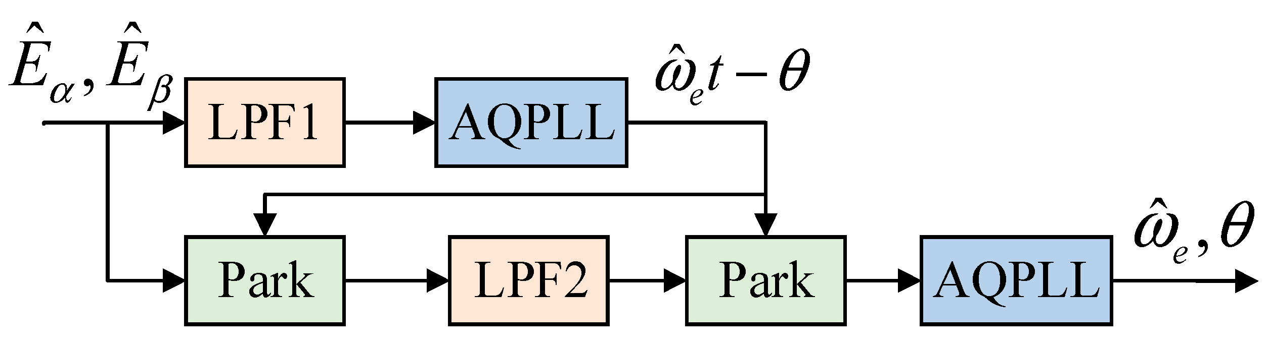
A novel Adaptive quadrature phase-locked loop (AQPLL) is used to estimate the rotor information. In order to solve the problems of low estimation accuracy and poor stability of the traditional phase-locked loop during the switching of motor speed, an improved adaptive quadrature phase-locked loop is used in this paper. The inverse potential normalization method is first used to eliminate the effect of speed variables on the phase-locked loop bandwidth, followed by the inclusion of a parameter adaptive tuning module based on the stochastic gradient descent method. Therefore, the new adaptive quadrature phase-locked loop is able to improve the speed tracking performance during speed switching and always maintain the stability of the motor.

2. PMSM Mathematical Model

The voltage equation of a surface mounted permanent magnet synchronous motor in a stationary α-β coordinate system can be expressed as:

$$\{\begin{array}{c}{u}_{\alpha }=R{i}_{\alpha }+L{\displaystyle \frac{d{i}_{\alpha }}{dt}}+E_{\alpha }\\ u_{\beta }=R{i}_{\beta }+L{\displaystyle \frac{d{i}_{\beta }}{dt}}+E_{\beta }\end{array}$$

(1)

The expression for the back EMF is given by:

$$\{\begin{array}{l}{E}_{\alpha }=-{\omega }_e{\psi }_f\sin {\theta }_e\hfill \\ E_{\beta }={\omega }_e{\psi }_f\cos {\theta }_e\hfill \end{array}$$

(2)

Rewrite Equation (1) as a current expression:

$$\{\begin{array}{c}{\displaystyle \frac{d{i}_{\alpha }}{dt}}={\displaystyle \frac{1}{L}}\left(u_{\alpha }-R{i}_{\alpha }-E_{\alpha }\right)\\ {\displaystyle \frac{d{i}_{\beta }}{dt}}={\displaystyle \frac{1}{L}}\left(u_{\beta }-R{i}_{\beta }-E_{\beta }\right)\end{array}$$

(3)

Equation (3) is discretized using the forward Euler method:

$$\{\begin{array}{c}{\displaystyle \frac{i_{\alpha }(k+1)-i_{\alpha }(k)}{T_s}}={\displaystyle \frac{1}{L}}\left[u_{\alpha }(k)-R{i}_{\alpha }(k)-E_{\alpha }(k)\right]\\ {\displaystyle \frac{i_{\beta }(k+1)-i_{\beta }(k)}{T_s}}={\displaystyle \frac{1}{L}}\left[u_{\beta }(k)-R{i}_{\beta }(k)-E_{\beta }(k)\right]\end{array}$$

(4)

Equation (4) is further simplified to Equation (5):

$$\{\begin{array}{c}{i}_{\alpha }(k+1)=\left[1-{\displaystyle \frac{T_{s}R}{L}}\right]i_{\alpha }(k)+{\displaystyle \frac{T_s}{L}}\left[u_{\alpha }(k)-E_{\alpha }(k)\right]\\ i_{\beta }(k+1)=\left[1-{\displaystyle \frac{T_{s}R}{L}}\right]i_{\beta }(k)+{\displaystyle \frac{T_s}{L}}\left[u_{\beta }(k)-E_{\beta }(k)\right]\end{array}$$

(5)

In Equation (5), u_α and u_β are the α-β axis components of the stator voltage; L = L_d = L_q is the d-q axis component of the stator inductance. R is the stator resistance; ω_e is the electrical angular velocity; i_α, i_β are the α-β axis components of the stator current. E_α, E_β are the extended back EMFs in the α-β axis system; Ψ_f is the rotor flux linkage; θ_e is the electrical angle, and t is the sampling time. i(k), u(k) and E(k) are the values of current, voltage, and extended back EMF, respectively, at time k. T_s denotes the sampling period of the discrete-time system.

In practice, the i_d* = 0 A control method is usually applied to surface-mounted permanent magnet synchronous motor drive systems. Figure 1 shows the overall block diagram of the control system in this paper. For the sensorless control system of the permanent magnet synchronous motor, in order to achieve its high-precision control requirements, the primary goal is to obtain the rotor information of the motor [27] and then feedback the position error to the controller for system control.

3. Adaptive Sliding Mode Algorithm

3.1. Traditional Super-Twisting Algorithms

The conventional super-twisting sliding mode observer model is shown in Equation (6):

$$\{\begin{array}{l}{\dot{\widehat{x}}}_1=-l_1{\left|{\overline{x}}_1\right|}^{1/2}sign({\overline{x}}_1)+x_2+{\rho }_1\hfill \\ {\dot{\widehat{x}}}_2=-l_{2}sign({\overline{x}}_1)+{\rho }_2\hfill \end{array}$$

(6)

where ${\dot{\widehat{x}}}_i$ is the estimated value of the state variable.

It has been shown in the literature [28] that the system converges and remains stable in finite time when Equation (6) satisfies the conditions of Equation (7) and l₁, l₂ satisfy the conditions of Equation (8):

$$\{\begin{array}{l}\left|{\rho }_1\right|\le {\delta }_1{\left|x_1\right|}^{1/2}\hfill \\ \left|{\rho }_2\right|\le {\delta }_2\hfill \end{array}$$

(7)

where δ₁, δ₂ are constants greater than zero.

$$\{\begin{array}{l}{l}_1>2{\delta }_1\hfill \\ l_2>k_1{\displaystyle \frac{5{\delta }_1{l}_1+6{\delta }_2+4{\left({\delta }_1+\frac{{\delta }_2}{l_1}\right)}^2}{2\left(l_1-2{\delta }_1\right)}}\hfill \end{array}$$

(8)

where k₁, k₂ are the observer gain parameters.

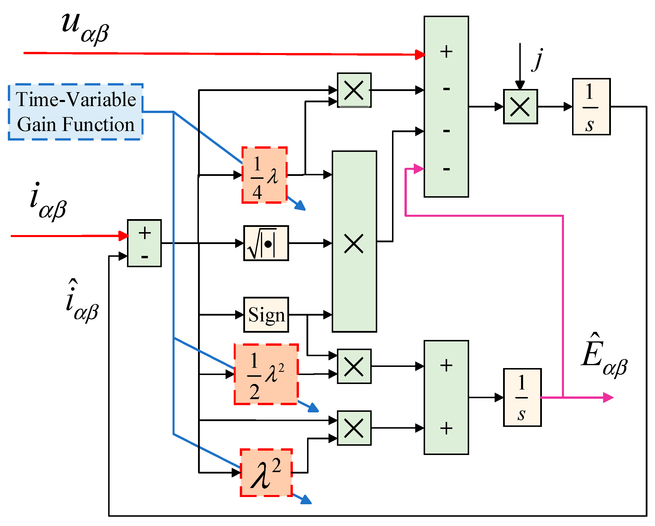
3.2. Gain Adaptive LSTA-SMO

Let 1/L = j, u_s = [u_α u_β]^T, i_s = [i_α i_β]^T, and E_s = [E_α E_β]^T. Since i_s and E_s are state variables, Equation (3) can be rewritten as Equation (9):

$$\{\begin{array}{l}{\dot{\mathit{i}}}_{\mathit{s}}=j\left({\mathit{u}}_{\mathit{s}}-R{\mathit{i}}_{\mathit{s}}-{\mathit{E}}_{\mathit{s}}\right)\hfill \\ {\dot{\mathit{E}}}_{\mathit{s}}=g\hfill \end{array}$$

(9)

where g denotes the derivative of the back EMF with respect to time.

Based on Equation (9) and the super-twisting algorithm model, the basic observer is designed as follows:

$$\{\begin{array}{l}{\dot{\hat{\mathit{i}}}}_{\mathit{s}}=j\left[{\mathit{u}}_{\mathit{s}}-R{\hat{\mathit{i}}}_{\mathit{s}}-{\hat{\mathit{E}}}_{\mathit{s}}-{\kappa }_1{\left|{\overline{\mathit{i}}}_{\mathit{s}}\right|}^{1/2}sign({\overline{\mathit{i}}}_{\mathit{s}})\right]\hfill \\ {\dot{\hat{\mathit{E}}}}_{\mathit{s}}={\kappa }_{2}sign({\overline{\mathit{i}}}_{\mathit{s}})\hfill \end{array}$$

(10)

where ${\hat{\mathit{i}}}_{\mathit{s}}$ and ${\hat{\mathit{E}}}_{\mathit{s}}$ are the estimated values of is and Es, respectively, ${\overline{\mathit{i}}}_{\mathit{s}}={\hat{\mathit{i}}}_{\mathit{s}}-{\mathit{i}}_{\mathit{s}}$,${\kappa }_1$ and ${\kappa }_2$ are the sliding mode gains.

According to the literature [28], it is known that the introduction of an additional linear gain term improves the recognition accuracy of the conventional super-twisting sliding mode algorithm. Therefore, an additional linear gain term is introduced in Equation (10) to obtain the LSTA–SMO expression (11):

$$\{\begin{array}{l}{\dot{\hat{\mathit{i}}}}_{\mathit{s}}=j\left[{\mathit{u}}_{\mathit{s}}-R{\hat{\mathit{i}}}_{\mathit{s}}-{\hat{\mathit{E}}}_{\mathit{s}}-k_1{\left|{\overline{\mathit{i}}}_{\mathit{s}}\right|}^{1/2}sign({\overline{\mathit{i}}}_s)-k_2{\overline{\mathit{i}}}_s\right]\hfill \\ {\dot{\hat{\mathit{E}}}}_{\mathit{s}}=k_{3}sign({\overline{\mathit{i}}}_{\mathit{s}})+k_4{\overline{\mathit{i}}}_{\mathit{s}}\hfill \end{array}$$

(11)

where kI have made modifications, kI have made modifications, I have made modifications, kI have made modifications are the observer gains.

The traditional STA–SMO and LSTA–SMO gains need to be solved in advance for the boundaries of the back EMF derivatives, which makes the algorithm debugging process cumbersome because it is difficult to find suitable gains to match them with different system boundaries.

3.3. AGFSTA–SMO

Based on the above gain mismatch, which leads to difficulties in debugging the algorithm, AGFSTA–SMO is proposed with the expression of Equation (12):

$$\{\begin{array}{l}{\dot{\hat{\mathit{i}}}}_{\mathit{s}}=j\left[{\mathit{u}}_{\mathit{s}}-R{\hat{\mathit{i}}}_{\mathit{s}}-{\hat{\mathit{E}}}_{\mathit{s}}-{\displaystyle \frac{1}{4}}\lambda {\left|{\overline{\mathit{i}}}_{\mathit{s}}\right|}^{1/2}sign({\overline{\mathit{i}}}_{\mathit{s}})-{\displaystyle \frac{1}{4}}\lambda {\overline{\mathit{i}}}_{\mathit{s}}\right]\hfill \\ {\dot{\hat{\mathit{E}}}}_{\mathit{s}}={\displaystyle \frac{1}{2}}{\lambda }^{2}sign({\overline{\mathit{i}}}_{\mathit{s}})+{\lambda }^2{\overline{\mathit{i}}}_{\mathit{s}}\hfill \end{array}$$

(12)

where λ is the time-varying gain function with respect to ${\overline{\mathit{i}}}_{\mathit{s}}$. The conditions in Equation (13) need to be satisfied when designing the gain function.

$$\{\begin{array}{l}\lambda =\left|h\right|\hfill \\ \dot{h}={\displaystyle \frac{\sigma }{e^{-{\overline{i}}_{\mathit{s}}}}}sign({\overline{\mathit{i}}}_s)\hfill \end{array}$$

(13)

where h is a time-varying gain function with respect to ${\overline{\mathit{i}}}_{\mathit{s}}$ and σ is a proportional integration factor that is a constant greater than zero.

In Equation (13), the initial value of λ needs to satisfy that λ > 0 is constant. Comparison of Equations (11) and (12) reveals that k₁ = k₂ = 0.25λ; k₃ = 0.5λ², and k₄ = λ².

Subtracting Equation (12) from Equation (9) gives the error Equation (14) for AGFSTA–SMO:

$$\{\begin{array}{l}{\dot{\overline{\mathit{i}}}}_{\mathit{\alpha }\mathit{\beta }}=j\left[-{\overline{\mathit{E}}}_{\mathit{s}}-{\displaystyle \frac{1}{4}}\lambda {\left|{\overline{\mathit{i}}}_{\mathit{s}}\right|}^{1/2}sign({\overline{\mathit{i}}}_{\mathit{s}})-{\displaystyle \frac{1}{4}}\lambda {\overline{\mathit{i}}}_{\mathit{s}}\right]\hfill \\ {\dot{\overline{\mathit{E}}}}_{\mathit{s}}={\displaystyle \frac{1}{2}}{\lambda }^2({\overline{\mathit{i}}}_{\mathit{s}})sign({\overline{\mathit{i}}}_s)+{\lambda }^2({\overline{\mathit{i}}}_{\mathit{s}}){\overline{\mathit{i}}}_{\mathit{s}}-g\hfill \end{array}$$

(14)

where ${\overline{\mathit{E}}}_{\mathit{s}}={\hat{\mathit{E}}}_{\mathit{s}}-{\mathit{E}}_{\mathit{s}}$.

${\dot{\overline{\mathit{E}}}}_{\mathit{s}}$ in Equation (14) is bounded. The parameter g in Equation (14) ranges from $\left|g\right|\le {\epsilon }_1+{\epsilon }_2\left|{\overline{\mathit{i}}}_{\mathit{s}}\right|$, where ε₁ and ε₂ are positive numbers.

The conclusion can be drawn from Equation (14):

For any initial values ${\overline{\mathit{i}}}_s$ and ${\overline{\mathit{E}}}_{\mathit{s}}$ of ${\overline{\mathit{i}}}_{\mathit{s}}\left(0\right)$ and ${\overline{\mathit{E}}}_{\mathit{s}}\left(0\right)$,${\overline{\mathit{i}}}_{\mathit{s}}$ and ${\overline{\mathit{E}}}_{\mathit{s}}$ converge in finite time if the designed time-varying gain function λ satisfies Equation (15).

$$\lambda >MAX\left(\sqrt{{\displaystyle \frac{32}{17}}{\epsilon }_1},\sqrt{{\displaystyle \frac{1}{2}}{\epsilon }_2},\sqrt{{\mathrm{H}}_1},\sqrt{{\mathrm{H}}_2}\right)$$

(15)

In the Equation (15), the relevant parameters are defined as follows:

$$\{\begin{array}{c}{\mathrm{H}}_1=-{\displaystyle \frac{b_1}{3a_1}}+2\sqrt{-{\varsigma }_1}\cos \left[\arccos \left({\displaystyle \frac{{\chi }_1}{{(-{\varsigma }_1)}^{3/2}}}\right)/3\right]\\ {\mathrm{H}}_2=-{\displaystyle \frac{b_2}{3a_2}}+2\sqrt{-{\varsigma }_2}\cos \left[\arccos \left({\displaystyle \frac{{\chi }_2}{{(-{\varsigma }_2)}^{3/2}}}\right)/3\right]\end{array}$$

(16)

$$\{\begin{array}{l}{a}_1=439\hfill \\ b_1=-3264{\epsilon }_1-512{\epsilon }_2\hfill \\ c_1=-37888{\epsilon }_1^2+3072{\epsilon }_1{\epsilon }_2\hfill \\ d_1=32768{\epsilon }_1^2{\epsilon }_2\hfill \\ \begin{array}{l}{\chi }_1=-{\displaystyle \frac{b_1^3}{27a_1^3}}-{\displaystyle \frac{d_1}{2a_1}}+{\displaystyle \frac{b_1{c}_1}{6a_1^2}}\\ {\varsigma }_1={\displaystyle \frac{c_1}{3a_1}}-{\displaystyle \frac{b_1^2}{9a_1^2}}\end{array}\hfill \end{array}and\{\begin{array}{l}{a}_2=5\hfill \\ b_2=-8{\epsilon }_1-15{\epsilon }_2\hfill \\ c_2=-80{\epsilon }_1^2+24{\epsilon }_1{\epsilon }_2\hfill \\ d_2=128{\epsilon }_1^2{\epsilon }_2\hfill \\ \begin{array}{l}{\chi }_2=-{\displaystyle \frac{b_2^3}{27a_2^3}}-{\displaystyle \frac{d_2}{2a_2}}+{\displaystyle \frac{b_2{c}_2}{6a_2^2}}\\ {\varsigma }_2={\displaystyle \frac{c_2}{3a_2}}-{\displaystyle \frac{b_2^2}{9a_2^2}}\end{array}\hfill \end{array}$$

(17)

3.4. Stability Proofs

Equation (18) is the new Lyapunov function with the following expression:

$$V={\displaystyle \frac{{\xi }^{T}P\xi }{{\lambda }^4}}$$

(18)

where the parameters ξ and P are defined in Equations (19) and (20), respectively.

$$\xi ={\left[\begin{array}{ccc}{\left|{\overline{\mathit{i}}}_{\mathit{s}}\right|}^{1/2}sign({\overline{\mathit{i}}}_{\mathit{s}})& {\overline{\mathit{i}}}_{\mathit{s}}& {\overline{\mathit{E}}}_{\mathit{s}}\end{array}\right]}^T$$

(19)

$$P={\displaystyle \frac{1}{2}}\left[\begin{array}{ccc}{\displaystyle \frac{33}{16}}{\lambda }^2& {\displaystyle \frac{1}{16}}{\lambda }^2& -{\displaystyle \frac{1}{4}}\lambda \\ {\displaystyle \frac{1}{16}}{\lambda }^2& {\displaystyle \frac{33}{16}}{\lambda }^2& -{\displaystyle \frac{1}{4}}\lambda \\ -{\displaystyle \frac{1}{4}}\lambda & -{\displaystyle \frac{1}{4}}\lambda & 2\end{array}\right]$$

(20)

Through Equation (18), Equation (21) can be further derived:

$$\{\begin{array}{l}\dot{V}={\dot{V}}_1+{\dot{V}}_2\hfill \\ {\dot{V}}_1={\xi }^T\dot{Q}\xi \hfill \\ {\dot{V}}_2=2{\xi }^{T}Q\xi \hfill \\ Q=P/\lambda \hfill \end{array}$$

(21)

From Equation (21), the proof of Lyapunov stability can be analyzed for both ${\dot{V}}_1$ and ${\dot{V}}_2$.

3.4.1. Analyze ${\dot{V}}_1$

Write the ${\dot{V}}_1$ expression:

$$\begin{array}{l}{\dot{V}}_1={\displaystyle \frac{1}{2}}{\xi }^T\left\{\dot{\lambda }\underset{N}{\underbrace{\left[\begin{array}{ccc}-{\displaystyle \frac{33}{8}}{\lambda }^{-3}& -{\displaystyle \frac{1}{8}}{\lambda }^{-3}& {\displaystyle \frac{3}{4}}{\lambda }^{-4}\\ -{\displaystyle \frac{1}{8}}{\lambda }^{-3}& -{\displaystyle \frac{33}{8}}{\lambda }^{-3}& {\displaystyle \frac{3}{4}}{\lambda }^{-4}\\ {\displaystyle \frac{3}{4}}{\lambda }^{-4}& {\displaystyle \frac{3}{4}}{\lambda }^{-4}& -8{\lambda }^{-5}\end{array}\right]}}\right\}\xi \\ ={\displaystyle \frac{1}{2}}\dot{\lambda }{\xi }^{T}N\xi \end{array}$$

(22)

Based on Equation (13), Equation (23) can be derived, so Equation (22) can be rewritten as Equation (24):

$$\dot{\lambda }=\dot{h}sign\left[h\right]\le \dot{h}\le {\displaystyle \frac{\sigma }{e^{-\left|{\overline{\mathit{i}}}_s\right|}}}$$

(23)

$${\dot{V}}_1={\displaystyle \frac{1}{2}}\dot{\lambda }{\xi }^{T}N\xi \le {\displaystyle \frac{1}{2}}\dot{h}{\xi }^{T}N\xi \le {\displaystyle \frac{\eta }{2e^{-\left|{\overline{\mathit{i}}}_s\right|}}}{\xi }^{T}N\xi$$

(24)

In Equation (24), because λ is always greater than 0, the N-matrix is positive definite, thus Equation (25) can be obtained:

$${\dot{V}}_1\le {\displaystyle \frac{\sigma }{2e^{-\left|{\overline{\mathit{i}}}_s\right|}}}{\xi }^{T}N\xi <0$$

(25)

3.4.2. Analyze ${\dot{V}}_2$

Write the ${\dot{V}}_2$ expression:

$$\{\begin{array}{l}{\dot{V}}_1=2{\dot{\xi }}^{T}Q\xi =-{\left|{\overline{\mathit{i}}}_{\mathit{s}}\right|}^{-1/2}{\xi }^T{y}_1\xi -{\xi }^T{y}_2\xi +y_3^T\xi \hfill \\ y_1={\displaystyle \frac{1}{8}}{\lambda }^{-3}\left[\begin{array}{ccc}17{\lambda }^2/16& 0& -\lambda /4\\ 0& 37{\lambda }^2/16& -3\lambda /4\\ -\lambda /4& -3\lambda /4& 1\end{array}\right]\hfill \\ y_2={\displaystyle \frac{1}{4}}{\lambda }^{-3}\left[\begin{array}{ccc}5{\lambda }^2/8& 0& 0\\ 0& 17{\lambda }^2/16& -\lambda /4\\ 0& -\lambda /4& 1\end{array}\right]\hfill \\ y_3^T=\left[\begin{array}{ccc}-g/4{\lambda }^3& -g/4{\lambda }^3& 2g/{\lambda }^4\end{array}\right]\hfill \end{array}$$

(26)

Equation (27) is the expression for the new variable η^T:

$${\mathit{\eta }}^T=\left[\begin{array}{ccc}{\left|{\overline{\mathit{i}}}_{\mathit{s}}\right|}^{{\displaystyle \frac{1}{2}}}& \left|{\overline{\mathit{i}}}_{\mathit{s}}\right|& \left|{\overline{\mathit{E}}}_{\mathit{s}}\right|\end{array}\right]$$

(27)

From the variable η^T and relation $\left|g\right|\le {\epsilon }_1+{\epsilon }_2\left|{\overline{\mathit{i}}}_{\mathit{s}}\right|$, Equation (28) can be derived:

$$\{\begin{array}{l}-{\left|{\overline{\mathit{i}}}_{\mathit{s}}\right|}^{-1/2}{\xi }^T{y}_1\xi -{\xi }^T{y}_2\xi \le -{\left|{\overline{\mathit{i}}}_{\mathit{s}}\right|}^{{\displaystyle \frac{1}{2}}}{\eta }^T{y}_1\eta -{\eta }^T{y}_2\eta \hfill \\ y_3^T\xi \le {\left|{\overline{\mathit{i}}}_{\mathit{s}}\right|}^{-1/2}{\eta }^T{\tau }_1\eta -{\eta }^T{\tau }_2\eta \hfill \end{array}$$

(28)

The parameters τ₁ and τ₂ in Equation (28) are defined as follows:

$${\tau }_1=\left[\begin{array}{ccc}{\epsilon }_1/4{\lambda }^3& 0& {\epsilon }_1/{\lambda }^4\\ 0& {\epsilon }_2/4{\lambda }^3& 0\\ {\epsilon }_1/{\lambda }^4& 0& 0\end{array}\right]$$

(29)

$${\tau }_2=\left[\begin{array}{ccc}{\epsilon }_1/4{\lambda }^3& 0& 0\\ 0& {\epsilon }_2/4{\lambda }^3& {\epsilon }_2/{\lambda }^4\\ 0& {\epsilon }_2/{\lambda }^4& 0\end{array}\right]$$

(30)

From Equations (26) and (28), the scaling equation for ${\dot{V}}_2$ is given as:

$$\begin{array}{ll}{\dot{V}}_2& =-{\left|{\overline{\mathit{i}}}_{\mathit{s}}\right|}^{-1/2}{\xi }^T{y}_1\xi -{\xi }^T{y}_2\xi +y_3^T\xi \\ & \le -{\left|{\overline{\mathit{i}}}_{\mathit{s}}\right|}^{-1/2}{\eta }^T\left(y_1-{\tau }_1\right)\eta -{\eta }^T\left(y_2-{\tau }_2\right)\eta \end{array}$$

(31)

Thus, it can be concluded that ${\dot{V}}_2$< 0 is constant when y₁-τ₁ and y₂-τ₂ are positive definite matrices. That is, ${\dot{V}}_2$< 0 is constant as long as the time-varying gain function λ satisfies Equation (15).

3.4.3. Consider the Following Factual Circumstances

$$\{\begin{array}{l}{\varphi }_{\min }\left\{Q\right\}{\Vert \xi \Vert }_2^2\le V={\xi }^{T}Q\xi \le {\varphi }_{\max }\left\{Q\right\}{\Vert \xi \Vert }_2^2\hfill \\ {\varphi }_{\min }\left\{y_1-{\tau }_1\right\}{\Vert \eta \Vert }_2^2\le {\eta }^T\left\{y_1-{\tau }_1\right\}\eta \le {\varphi }_{\max }\left\{y_1-{\tau }_1\right\}{\Vert \eta \Vert }_2^2\hfill \end{array}$$

(32)

where max{·} and min{·} denote the maximum and minimum eigenvalues of the matrix, respectively; and ${\Vert \cdot \Vert }_2^2$ denotes the Euclidean norm.

The range of Euclidean paradigms for ξ is given by Equation (32):

$${\left|{\overline{\mathit{i}}}_{\mathit{s}}\right|}^{1/2}\le {\Vert \xi \Vert }_2\le {\displaystyle \frac{V^{1/2}}{{\varphi }_{\min }^{1/2}\left\{Q\right\}}}$$

(33)

Therefore, Equation (31) can be rewritten as Equation (34):

$$\begin{array}{ll}{\dot{V}}_2& \le -{\left|{\overline{\mathit{i}}}_{\mathit{s}}\right|}^{-1/2}{\eta }^T\left\{y_1-{\tau }_1\right\}\eta -{\eta }^T\left\{y_2-{\tau }_2\right\}\eta \\ & \le -{\left|{\overline{\mathit{i}}}_{\mathit{s}}\right|}^{-1/2}{\eta }^T\left\{y_1-{\tau }_1\right\}\eta \\ & \le -{\left|{\overline{\mathit{i}}}_{\mathit{s}}\right|}^{-1/2}{\varphi }_{\min }\left\{y_1-{\tau }_1\right\}{\Vert \eta \Vert }_2^2\\ & =-{\left|{\overline{\mathit{i}}}_{\mathit{s}}\right|}^{-1/2}{\varphi }_{\min }\left\{y_1-{\tau }_1\right\}{\Vert \xi \Vert }_2^2\\ & \le -{\displaystyle \frac{{\varphi }_{\min }^{1/2}\left\{Q\right\}{\varphi }_{\min }\left\{y_1-{\tau }_1\right\}}{V^{1/2}{\varphi }_{\max }\left\{Q\right\}}}V\\ & =-{\displaystyle \frac{{\varphi }_{\min }^{1/2}\left\{Q\right\}{\varphi }_{\min }\left\{y_1-{\tau }_1\right\}}{{\varphi }_{\max }\left\{Q\right\}}}{V}^{1/2}\end{array}$$

(34)

Equation (35) can be derived from Equation (34):

$$\dot{V}={\dot{V}}_1+{\dot{V}}_2<{\dot{V}}_2\le -{\displaystyle \frac{{\varphi }_{\min }^{1/2}\left\{Q\right\}{\varphi }_{\min }\left\{y_1-{\tau }_1\right\}}{{\varphi }_{\max }\left\{Q\right\}}}{V}^{1/2}$$

(35)

It is worth noting that the system can converge only when the time-varying gain function λ satisfies the condition Equation (15). This also means that the conditions of Equation (13) need to be satisfied at all times when the value λ is increased to the point where Equation (15) holds, and finally the system is proved to converge based on Equation (35).

Therefore, it can be concluded that ${\overline{\mathit{i}}}_{\mathit{s}}$ and ${\overline{\mathit{E}}}_{\mathit{s}}$ can converge to zero in finite time and the proof ends. Figure 2 shows the schematic block diagram of AGFSTA–SMO proposed in this paper.

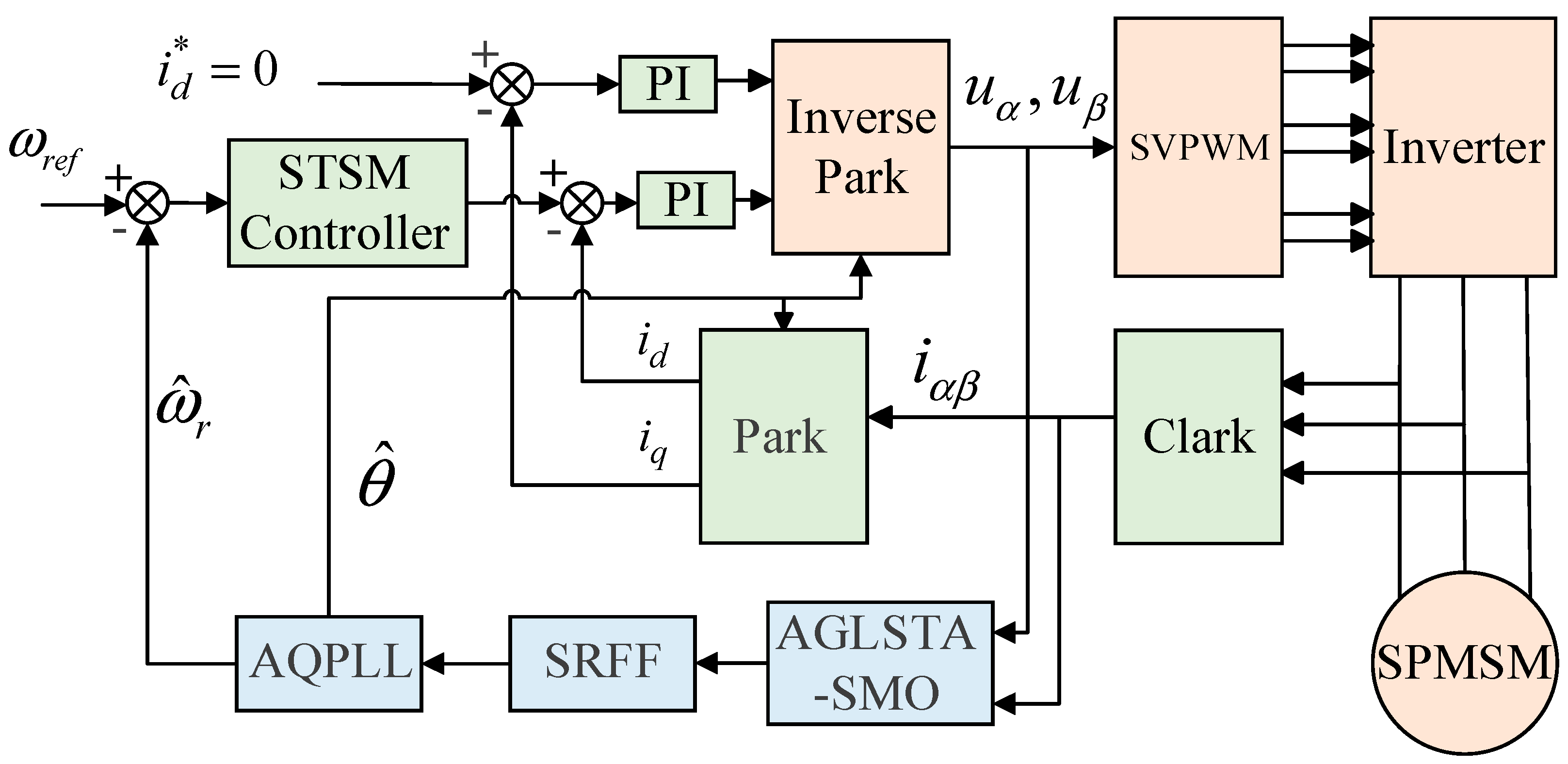
4. Rotor Information Extraction Program

4.1. Synchronized Reference System Filter

Due to the existence of a large number of high harmonics in the extended back EMF waveform observed by the traditional STA–SMO, the observation accuracy will be greatly affected when the motor is running at high speed. In order to improve the observation accuracy and reduce the amplitude of jitter, this paper adopts the SRFF to filter out the harmonic components in the extended back EMF waveform.

The SRFF designed in this paper is based on the characteristics of space vector control of permanent magnet synchronous motor, which firstly uses Park transform to change the back EMF into direct current, then low-pass filtering, and finally uses inverse Park transform to AC quantity. Due to the characteristics of space vector control, this method is not only able to filter out the high-frequency components in the back EMF waveform, but also able to ensure the phase stability of the system [29]. The block diagram of SRFF is shown in Figure 3.

The back EMFs ${\widehat{E}}_{\alpha }$ and ${\widehat{E}}_{\beta }$ pass through the low-pass filter LPF1 into an adaptive quadrature phase-locked loop [30]. Let the phase lag angle due to LPF1 be Δθ. Thus, the extended back EMF can be expressed as a superposition of the fundamental and the higher harmonics, and Equation (36) is the expression for the extended back EMF:

$$\{\begin{array}{l}{\widehat{E}}_{\alpha }(t)=-K_0\sin \left({\widehat{\omega }}_{e}t\right)+{\displaystyle \sum _{x=2}^{\infty }{K}_x\sin \left(x{\widehat{\omega }}_{e}t+\Delta \theta \right)}\hfill \\ {\widehat{E}}_{\beta }(t)=K_0\cos \left({\widehat{\omega }}_{e}t\right)+{\displaystyle \sum _{x=2}^{\infty }{K}_x\sin \left(x{\widehat{\omega }}_{e}t+\Delta \theta \right)}\hfill \end{array}$$

(36)

where ${\widehat{\omega }}_{e}t$ is the fundamental phase angle, K₀ is the fundamental amplitude, $x{\widehat{\omega }}_{e}t$ is the harmonic phase, and K_x is the harmonic amplitude.

The back EMF base wave is Park transformed to give Equation (37):

$$\left[\begin{array}{c}{\widehat{E}}_d\\ {\widehat{E}}_q\end{array}\right]=\left[\begin{array}{cc}\cos \left({\widehat{\omega }}_{e}t-\Delta \theta \right)& \sin \left({\widehat{\omega }}_{e}t-\Delta \theta \right)\\ -\sin \left({\widehat{\omega }}_{e}t-\Delta \theta \right)& \cos \left({\widehat{\omega }}_{e}t-\Delta \theta \right)\end{array}\right]\left[\begin{array}{c}-K_0\sin \left({\widehat{\omega }}_{e}t\right)\\ K_0\cos \left({\widehat{\omega }}_{e}t\right)\end{array}\right]=\left[\begin{array}{c}-K_0\sin \left(\Delta \theta \right)\\ K_0\cos \left(\Delta \theta \right)\end{array}\right]$$

(37)

Since K₀ is only related to the electrical angular frequency and the rotor flux linkage, and the error angle Δθ is only related to the electrical angular frequency and the filter LPF1 cutoff frequency, both K₀ and Δθ remain constant after the rotational speed is stabilized, i.e., the base wave of the back EMF is changed to a straight flow. After passing through the low-pass filter LPF2, there is no phase lag in the fundamental wave component of this reaction potential.

Equation (38) can be obtained after Park’s inverse transformation:

$$\left[\begin{array}{c}{\widehat{E}}_{\alpha }\\ {\widehat{E}}_{\beta }\end{array}\right]={\left[\begin{array}{cc}\cos \left({\widehat{\omega }}_{e}t-\theta \right)& \sin \left({\widehat{\omega }}_{e}t-\Delta \theta \right)\\ -\sin \left({\widehat{\omega }}_{e}t-\theta \right)& \cos \left({\widehat{\omega }}_{e}t-\Delta \theta \right)\end{array}\right]}^{-1}\left[\begin{array}{c}-K_0\sin \left(\Delta \theta \right)\\ K_0\cos \left(\Delta \theta \right)\end{array}\right]=\left[\begin{array}{c}-K_0\sin \left({\widehat{\omega }}_{e}t\right)\\ K_0\cos \left({\widehat{\omega }}_{e}t\right)\end{array}\right]$$

(38)

From the above derivation, it can be concluded that when the filtering is performed in the d-q axis, the filter does not affect the amplitude phase of the fundamental wave, since the fundamental wave is transformed into a straight flow and also accounts for the unobserved angular lag. The high-frequency harmonics are still AC quantities after Park’s transform, so they can be filtered out by the low-pass filter, which in turn reduces system jitter.

4.2. Adaptive Quadrature Phase-Locked Loop

Since the conventional phase-locked loop is affected by its own characteristics during the switching of the motor speed, it ensures the stability of the system while failing to maintain a low phase delay [31]. Therefore, in this paper, the estimation strategy of adaptive quadrature phase-locked loop is used in the rotor information extraction part. Figure 4 shows the schematic diagram of the AQPLL.

First, the back EMF of the AGFSTA–SMO output is normalized:

$${\hat{\mathit{E}}}_{\mathit{n}}={\hat{\mathit{E}}}_{\mathit{s}}/\sqrt{E_{\alpha }^2+E_{\beta }^2}$$

(39)

where ${\hat{\mathit{E}}}_{\mathit{n}}={\left[\begin{array}{cc}{\widehat{E}}_{n\alpha }& {\widehat{E}}_{n\beta }\end{array}\right]}^T$.

After processing through Equation (39), the rotational speed variable will no longer affect the calculation of the phase-locked loop bandwidth. Equation (40) is the transfer function of the adaptive quadrature phase-locked loop:

$$G_{PLL}\left(s\right)={\displaystyle \frac{k_{p}s+k_i}{s^2+k_{p}s+k_i}}$$

(40)

The AQPLL adaptive strategy designed based on stochastic gradient descent method is designed to minimize the squared error of the controller input by adjusting the adaptive gains k_p and k_i. Therefore, the poles of Equation (40) can be replaced by Equation (41):

$$k_p\left[h\right]=2\zeta \upsilon \left[h\right],k_i\left[h\right]={\upsilon }^2\left[h\right]$$

(41)

where ζ is the damping factor, h is the discrete time step parameter, and $\upsilon$ is the intrinsic frequency, i.e., the AQPLL tuning parameter.

Since ζ is a constant and the phase-locked loop bandwidth is related to $\upsilon$, the adaptive strategy for the AQPLL parameters can be expressed as Equation (42):

$$\upsilon \left[h\right]=\upsilon \left[h-1\right]-\iota {\displaystyle \frac{1}{2}}\left({\displaystyle \frac{\partial o^2\left[h\right]}{\partial \upsilon \left[h-1\right]}}\right)$$

(42)

where $\iota$ is the step parameter that determines the speed of adaptive tuning and $o$ is the input error of the PI controller.

By solving Equation (42), the expression for updating the tuning parameters can be obtained as:

$$\upsilon \left[h\right]=\upsilon \left[h-1\right]-\iota w_1\left[h\right]w_2\left[h\right]=\upsilon \left[h-1\right]-\Delta \upsilon \left[h\right]$$

(43)

where $\Delta \upsilon \left[h\right]$ is the step increment, and w₁ and w₂ are partial solutions with the following expressions:

$$\{\begin{array}{c}{w}_1\left[h\right]={\widehat{E}}_{\alpha }^f\left[h\right]\sin \left(\widehat{\theta }\left[h-1\right]\right)-{\widehat{E}}_{\beta }^f\left[h\right]\cos \left(\widehat{\theta }\left[h-1\right]\right)\\ w_2\left[h\right]=2\zeta o\left[h-1\right]+T_s\upsilon \left[h-1\right]\left(o\left[h-1\right]-o\left[h-2\right]\right)\end{array}$$

(44)

where ${\widehat{E}}_{\alpha }^f$ and ${\widehat{E}}_{\beta }^f$ are the estimated values of the inverse electromotive force after filtering.

5. Simulation and Experimental Verification

In order to verify the advantages of the AGFSTA–SMO algorithm, this paper establishes two different position sensorless control models for permanent magnet synchronous motors in Simulink: a linear gain super-twisting sliding mode observer and a parameter adaptive finite time super-twisting sliding mode observer. The motor rotor information extraction results are analyzed in terms of rotational speed tracking, rotational speed error, rotor position tracking, rotor position error, and sudden load increase/decrease to further validate the advantages of the AGFSTA–SMO algorithm over the LSTA–SMO and conventional STA–SMO algorithms.

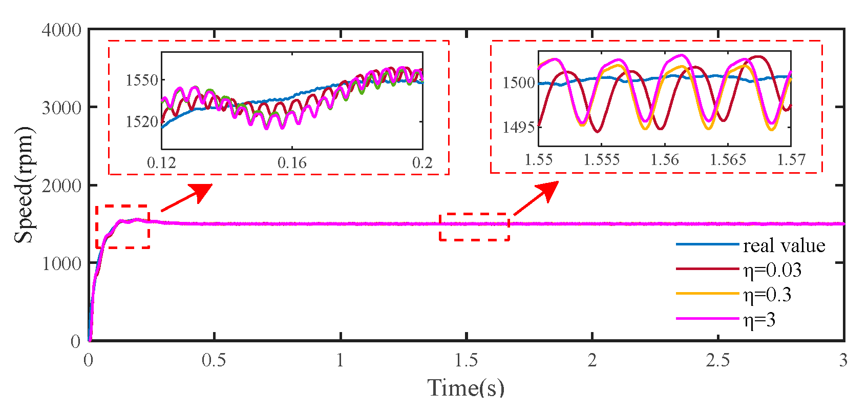
5.1. Simulation Analysis

The parameters of the mounted permanent magnet synchronous motor used for the simulation and experimentation are provided by the motor manufacturer, as shown in

Table 1. Motor parameters and gain parameters.

Items	Values	Parameters	Values
Stator winding resistance Rs	0.56 Ω	k1	100
Stator winding inductance LS	0.62 mH	k2	400
Flux linkage ψf	0.0125 Wb	k3	100
Rotational inertia J	1.5 kg·cm2	k4	50
Pole pairs p	4	λ	0.001
Rated power	250 W	Rated current	7.5 A
Rated toque	0.796 N·m	Rated speed	3000 rpm

. In the simulation process, in order to show the difference between the two observation algorithms more intuitively, the parameters of the current loop and speed loop controllers in the two models are set to be the same, the simulation time of the system is fixed to be 3 s, and the fixed step size is set to be 1 μs.

As can be seen from Figure 5, the AGFSTA–SMO algorithm has a higher speed tracking accuracy during motor acceleration when the target speeds are 1000 rpm, 1500 rpm, and 2000 rpm, respectively, and the estimated speeds are able to track the target speeds faster and maintain a relatively small jitter amplitude after that. As a result, the AGFSTA–SMO algorithm has a higher speed tracking accuracy and faster convergence despite the different target speeds of the motors.

As can be seen in Figure 6, when the target speed of the motor differs from the actual speed, AGFSTA–SMO is able to adjust the sliding mode gain more quickly, and quickly reduce the error between the estimated speed and the actual speed. When the motor reaches the target speed, the AGFSTA–SMO algorithm limits the sliding mode gain to a certain range based on the motor’s speed, which reduces speed overshoot. Therefore, when the motor reaches the target speed, the AGFSTA–SMO algorithm has less fluctuation in the speed error and the absolute value of the error is smaller, which makes it easier to control the motor.

From the theory of sliding mode control, it can be seen that the system’s ability to resist disturbances mainly depends on the sliding mode gain, i.e., when the system encounters disturbances, it can be quickly restored to a stable state by adjusting the sliding mode gain. Figure 7 shows the speed tracking of the motor during sudden load application. As can be seen from Figure 7, when a load perturbation of T_L = 0.2 N·m is applied abruptly at 1 s, the estimated speed obtained by the AGFSTA–SMO algorithm is able to track the actual speed more quickly and maintain a smaller error during the recovery to the target speed. Therefore, the tracking performance of the AGFSTA–SMO is superior to the existing LSTA–SMO when the motor is in a loaded condition.

Figure 8 is able to further validate the speed tracking ability of both algorithms when a sudden load is applied. From the results demonstrated in Figure 8, it can be seen that AGFSTA–SMO is able to adjust the sliding mode gain more quickly when there is a sudden change in the operating conditions of the motor, so that the estimated rotational speed quickly tracks the actual rotational speed. It can be concluded that the AGFSTA–SMO observer proposed in this paper has a significant advantage over LSTA–SMO under multiple operating conditions of the motor.

As can be seen from Figure 9, the position sensorless control system reaches a steady state at 0.1 s. The rotor position estimated by the algorithm always fluctuates up and down around the true value due to the accelerated frequency change of the position waveform as a result of the motor rotating too fast. It can thus be shown that the AGFSTA–SMO algorithm is always able to accurately estimate the rotor position and stabilize the error within 0.1 rad when the target speed of the motor is different.

As can be seen from Figure 10, when the load is applied abruptly at 1 s, the actual rotor position changes abruptly, but it is estimated that the rotor position will still maintain the previous motion trend for a short period of time. As a result, the position error increases slightly for a short period of time, then immediately retraces its steps and eventually reaches a steady state. When the motor is adjusted to a stable state, the rotor position error obtained by the AGFSTA–SMO algorithm remains within 0.1 rad, which verifies the feasibility of the algorithm under different working conditions.

From the comparison of the simulation results of the two algorithms, it can be seen that the AGFSTA–SMO algorithm not only has better tracking performance, but also has a higher estimation accuracy. In addition, since the sliding mode gain of AGFSTA–SMO is related to the motor speed, the algorithm is able to respond quickly to the sudden change of the motor condition, avoiding the further expansion of the error in time and ensuring the stability of the control system.

From Figure 11, it can be seen that when the sliding mode gain λ is 0.03, the speed tracking effect is the best, and the tracking ability of the speed is strongest under the loaded working condition. The value of 0.03 for the algorithmic gain is just an example to give the reader an idea of the output results for each magnitude of gain.

5.2. Experimental Verification Analysis

In order to further test the performance of AGFSTA–SMO, an experimental platform for permanent magnet synchronous motor control system was constructed as shown in Figure 12. In this study, the position sensorless vector control strategy was realized by using an STM32F407 microcontroller.

5.2.1. No-Load Experiment

Figure 13 represents the waveform of rotor position when the rotor rises from the stationary state to the target speed. The target speed is set to 1000 rpm, 1500 rpm, and 2000 rpm, and the sliding mode gain λ is set to 0.001.

Figure 13 shows the dynamic performance test results for target speeds of 1000 rpm, 1500 rpm, and 2000 rpm, respectively. Due to the delay in data transmission from the upper computer, the rotor position waveform in Figure 13 only represents the rotor position waveform at a time of approximately 0.1 s. The Hall sensor is used to read the actual rotor position information during the test, which is used to verify the correctness of the estimated rotor position, and the AGFSTA–SMO algorithm is used to estimate the rotor position using AQPLL. As can be seen in Figure 13, the estimates obtained by the AGFSTA–SMO algorithm still float around the true value, except for the errors caused by the mechanical characteristics of the Hall sensors. The relatively small amplitude of the back EMF in the low-speed range with respect to the gain of the AGFSTA–SMO leads to poor accuracy in estimating the rotor position during the low-speed operation of the motor. Therefore, when the motor speed is increased to 2000 rpm, the oscillations in the estimated rotor position are significantly reduced and the estimation accuracy is significantly improved.

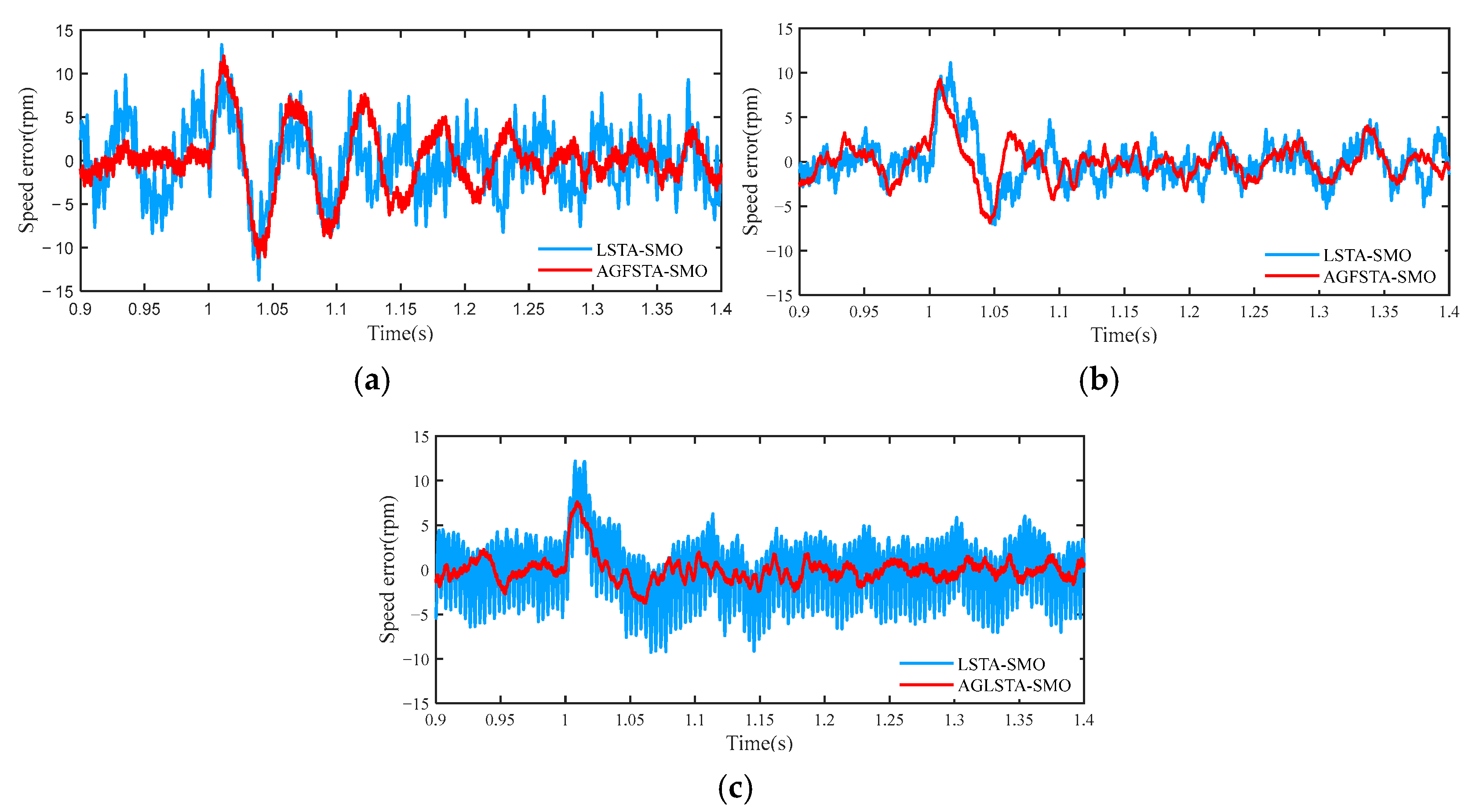
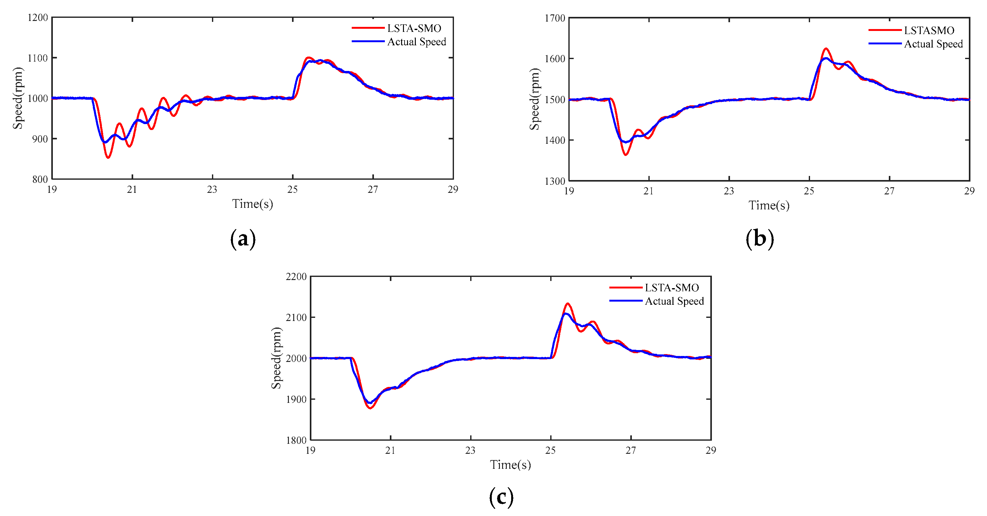
5.2.2. Comparison of Speed Tracking Performance of LSTA–SMO Algorithm and AGFSTA–SMO Algorithm under Sudden Load Change Conditions

As can be seen in Figure 14, the sudden change in motor load results in increasing the jitter amplitude of the observations due to the constant sliding mode gain of the LSTA–SMO algorithm, which further leads to oscillations in the outputs of the LSTA–SMO, resulting in a decrease in the accuracy of the estimation of the rotor position and speed, and is particularly prominent in the low-speed domain. When the rotational speed is increased to 1500 rpm and 2000 rpm, the LSTA–SMO gain is increased, thus resulting in a faster convergence of the observations and a reduction in the jitter amplitude. As can be seen in Figure 15, when the AGFSTA–SMO algorithm is used, the sliding mode observer gain can be adjusted adaptively according to the motor speed, and the original chattering of the sliding mode can be suppressed. Therefore, the AGFSTA–SMO algorithm has a better performance in terms of jitter amplitude, convergence speed, and jitter frequency when the motor operating conditions change abruptly.

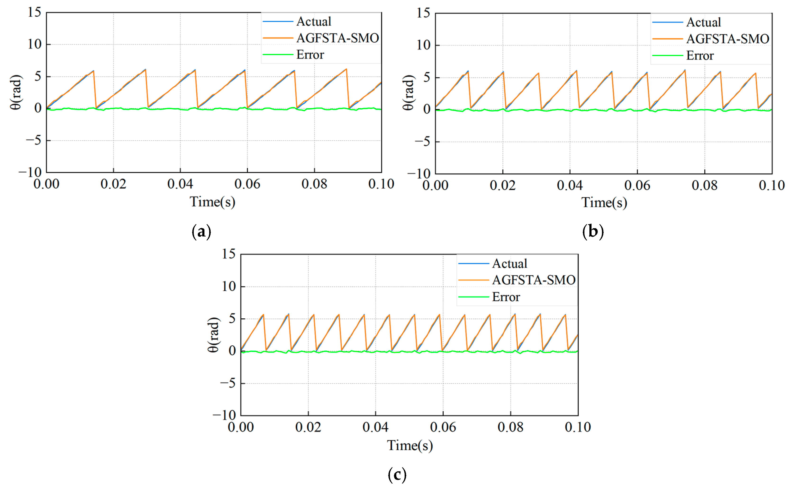
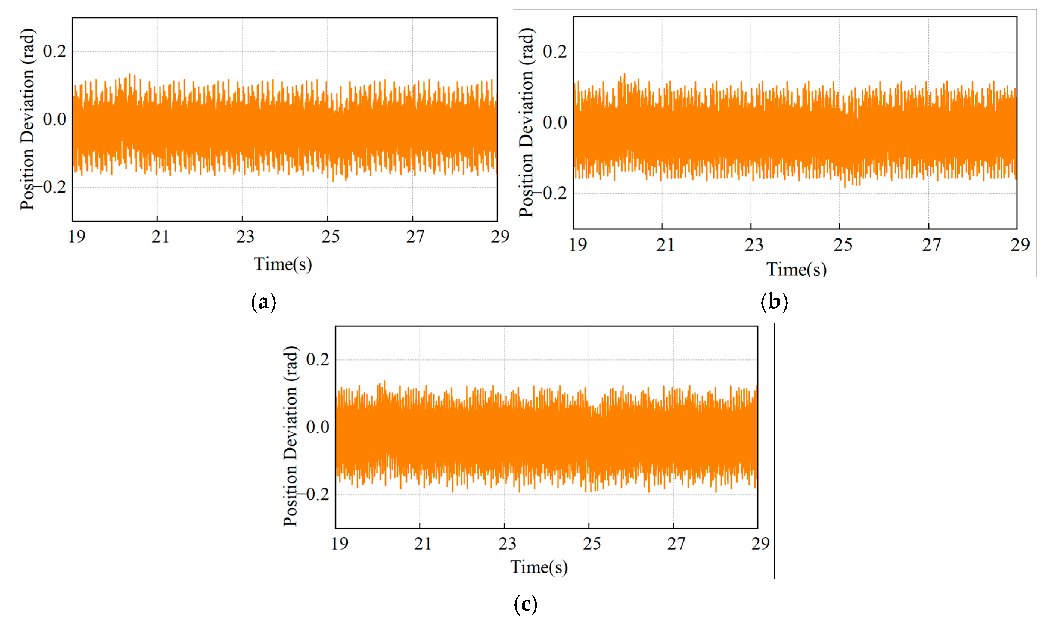
5.2.3. Performance of AGFSTA–SMO Method for Rotor Position Estimation during Sudden Load Changes

From Figure 16, it can be seen that when the motor is suddenly loaded at 25 s, the error between the estimated rotor position and the actual rotor position increases by 0.05 rad, and the recovery time is about 0.6 s. Therefore, the effect of the perturbation of the load on the estimation accuracy can be almost ignored.

6. Conclusions

In this paper, a simple and efficient sensorless control strategy is proposed for the permanent magnet synchronous motor drive control system. Compared with the traditional super-twisting sliding mode observer and the improved super-twisting sliding mode observer, the proposed AGFSTA–SMO is able to improve the sliding mode convergence rate by using the gain adaptive parameter, which solves the problem of the difficulty in parameter adjustment due to the excessive number of gains in the traditional model. It also simplifies the parameter adjustment process by designing the rotational speed-dependent adaptive function to replace the multiple gain parameters in the super-twisting sliding mode observer In addition, the observation accuracy is improved. Meanwhile, this paper reduces the negative impact of harmonic components by using synchronized reference system filters and adaptive quadrature phase-locked loops, which further improves the convergence speed of the observer and reduces the jitter amplitude of the observation results. Finally, the Lyapunov theory was used to demonstrate the steady state nature of the sensorless control system for permanent magnet synchronous motors. Numerous experimental results validated the advantages of the scheme proposed in this paper. In future research, work will be focused on improving the situation of the large error and difficult startup of the downward sliding mode observer in the low-speed domain, and extending the method proposed in this paper to the low-speed domain.

References

1. Wang, Y.; Xu, Y.; Zou, J. Sliding-mode sensorless control of PMSM with inverter nonlinearity compensation. IEEE Trans. Power Electron. 2019, 34, 10206–10220. [Google Scholar] [CrossRef]
2. Gong, C.; Hu, Y.; Gao, J.; Wang, Y.; Yan, L. An improved delay-suppressed sliding-mode observer for sensorless vector-controlled PMSM. IEEE Trans. Ind. Electron. 2019, 67, 5913–5923. [Google Scholar] [CrossRef]
3. Wang, Y.; Wang, X.; Xie, W.; Dou, M. Full-speed range encoderless control for salient-pole PMSM with a novel full-order SMO. Energies 2018, 11, 2423. [Google Scholar] [CrossRef]
4. Apte, A.; Joshi, V.A.; Mehta, H.; Walambe, R. Disturbance-observer-based sensorless control of PMSM using integral state feedback controller. IEEE Trans. Power Electron. 2019, 35, 6082–6090. [Google Scholar] [CrossRef]
5. Volpato Filho, C.J.; Xiao, D.; Vieira, R.P.; Emadi, A. Observers for high-speed sensorless pmsm drives: Design methods, tuning challenges and future trends. IEEE Access 2021, 9, 56397–56415. [Google Scholar] [CrossRef]
6. Yin, Z.; Zhang, Y.; Cao, X.; Yuan, D.; Liu, J. Estimated position error suppression using novel PLL for IPMSM sensorless drives based on full-order SMO. IEEE Trans. Power Electron. 2021, 37, 4463–4474. [Google Scholar] [CrossRef]
7. Chen, Z.; Zhang, X.; Zhang, H.; Liu, C.; Luo, G. Adaptive sliding mode observer-based sensorless control for SPMSM employing a dual-PLL. IEEE Trans. Transp. Electrif. 2021, 8, 1267–1277. [Google Scholar] [CrossRef]
8. Ni, Y.; Shao, D. Research of improved mras based sensorless control of permanent magnet synchronous motor considering parameter sensitivity. In Proceedings of the 2021 IEEE 4th Advanced Information Management, Communicates, Electronic and Automation Control Conference (IMCEC), Chongqing, China, 18–20 June 2021; Volume 4, pp. 633–638. [Google Scholar]
9. Zerdali, E.; Barut, M. The comparisons of optimized extended Kalman filters for speed-sensorless control of induction motors. IEEE Trans. Ind. Electron. 2017, 64, 4340–4351. [Google Scholar] [CrossRef]
10. Nurettin, A.; İnanç, N. Sensorless vector control for induction motor drive at very low and zero speeds based on an adaptive-gain super-twisting sliding mode observer. IEEE J. Emerg. Sel. Top. Power Electron. 2023, 11, 4332–4339. [Google Scholar] [CrossRef]
11. Benevieri, A.; Formentini, A.; Marchesoni, M.; Passalacqua, M.; Vaccaro, L. Sensorless control with switching frequency square wave voltage injection for SPMSM with low rotor magnetic anisotropy. IEEE Trans. Power Electron. 2023, 38, 10060–10072. [Google Scholar] [CrossRef]
12. Xu, W.; Qu, S.; Zhao, L.; Zhang, H. An improved adaptive sliding mode observer for middle-and high-speed rotor tracking. IEEE Trans. Power Electron. 2020, 36, 1043–1053. [Google Scholar] [CrossRef]
13. Zuo, Y.; Lai, C.; Iyer, K.L.V. A review of sliding mode observer based sensorless control methods for PMSM drive. IEEE Trans. Power Electron. 2023, 38, 11352–11367. [Google Scholar] [CrossRef]
14. Ren, N.; Fan, L.; Zhang, Z. Sensorless PMSM control with sliding mode observer based on sigmoid function. J. Electr. Eng. Technol. 2021, 16, 933–939. [Google Scholar] [CrossRef]
15. Jin, D.; Liu, L.; Lin, Q.; Liang, D. Sensorless Control Strategy of PMSM with Disturbance Rejection Based on Adaptive Sliding Mode Control Law. IEEE Trans. Transp. Electrif. 2023, 10, 5424–5438. [Google Scholar] [CrossRef]
16. Wang, C.; Gou, L.; Dong, S.; Zhou, M.; You, X. Sensorless control of IPMSM based on super-twisting sliding mode observer with CVGI considering flying start. IEEE Trans. Transp. Electrif. 2021, 8, 2106–2117. [Google Scholar] [CrossRef]
17. Ge, Y.; Yang, L.; Ma, X. A harmonic compensation method for SPMSM sensorless control based on the orthogonal master-slave adaptive notch filter. IEEE Trans. Power Electron. 2021, 36, 11701–11711. [Google Scholar] [CrossRef]
18. Chen, L.; Jin, Z.; Shao, K.; Wang, H.; Wang, G.; Iu, H.H.; Fernando, T. Sensorless Fixed-time Sliding Mode Control of PMSM Based on Barrier Function Adaptive Super-Twisting Observer. IEEE Trans. Power Electron. 2023, 39, 3037–3051. [Google Scholar] [CrossRef]
19. Yang, C.; Song, B.; Xie, Y.; Zheng, S.; Tang, X. Adaptive Identification of Nonlinear Friction and Load Torque for PMSM Drives via a Parallel-Observer-Based Network with Model Compensation. IEEE Trans. Power Electron. 2023, 38, 5875–5897. [Google Scholar] [CrossRef]
20. Jiang, T.; Ni, R.; Gu, S.; Wang, G. A study on position estimation error in sensorless control of PMSM based on back EMF observation method. In Proceedings of the 2021 24th International Conference on Electrical Machines and Systems (ICEMS), Gyeongju, Republic of Korea, 31 October–3 November 2021; pp. 1999–2003. [Google Scholar]
21. Chen, Y.; Li, M.; Gao, Y.W.; Chen, Z.Y. A sliding mode speed and position observer for a surface-mounted PMSM. ISA Trans. 2019, 87, 17–27. [Google Scholar] [CrossRef]
22. Wang, B.; Shao, Y.; Yu, Y.; Dong, Q.; Yun, Z.; Xu, D. High-order terminal sliding-mode observer for chattering suppression and finite-time convergence in sensorless SPMSM drives. IEEE Trans. Power Electron. 2021, 36, 11910–11920. [Google Scholar] [CrossRef]
23. Yang, Z.; Ding, Q.; Sun, X.; Lu, C.; Zhu, H. Speed sensorless control of a bearingless induction motor based on sliding mode observer and phase-locked loop. ISA Trans. 2022, 123, 346–356. [Google Scholar] [CrossRef] [PubMed]
24. Xu, W.; Qu, S.; Zhang, H. A composite sliding-mode observer with PLL structure for a sensorless SPMSM system. Int. J. Electr. Power Energy Syst. 2022, 143, 108510. [Google Scholar] [CrossRef]
25. Naderian, M.; Markadeh, G.A.; Karimi-Ghartemani, M.; Mojiri, M. Improved sensorless control strategy for IPMSM using an ePLL approach with high-frequency injection. IEEE Trans. Ind. Electron. 2023, 71, 2231–2241. [Google Scholar] [CrossRef]
26. Hou, Q.; Ding, S.; Dou, W.; Jiang, L. Estimated Position Error Suppression Using Quasi-Super-Twisting Observer and Enhanced Quadrature Phase-Locked Loop for PMSM Sensorless Drives. IEEE Trans. Circuits Syst. II Express Briefs 2024, 71, 3865–3869. [Google Scholar] [CrossRef]
27. Zhu, W.; Li, S.; Du, H.; Yu, X. Nonsmooth observer-based sensorless speed control for permanent magnet synchronous motor. IEEE Trans. Ind. Electron. 2022, 69, 13514–13523. [Google Scholar] [CrossRef]
28. Moreno, J.A.; Osorio, M. A Lyapunov approach to second-order sliding mode controllers and observers. In Proceedings of the 2008 47th IEEE conference on decision and control, Cancun, Mexico, 9–11 December 2008; pp. 2856–2861. [Google Scholar]
29. Lin, S.; Zhang, W. An adaptive sliding-mode observer with a tangent function-based PLL structure for position sensorless PMSM drives. Int. J. Electr. Power Energy Syst. 2017, 88, 63–74. [Google Scholar] [CrossRef]
30. Novak, Z.; Novak, M. Adaptive PLL-based sensorless control for improved dynamics of high-speed PMSM. IEEE Trans. Power Electron. 2022, 37, 10154–10165. [Google Scholar] [CrossRef]
31. Liu, G.; Zhang, H.; Song, X. Position-estimation deviation-suppression technology of PMSM combining phase self-compensation SMO and feed-forward PLL. IEEE J. Emerg. Sel. Top. Power Electron. 2020, 9, 335–344. [Google Scholar] [CrossRef]
Figure 1. Block diagram of permanent magnet synchronous motor control system.
Actuators 13 00395 g001
Figure 2. Block diagram of AGFSTA-SMO.
Actuators 13 00395 g002
Figure 3. Block diagram of SRFF structure.
Actuators 13 00395 g003
Figure 4. Schematic diagram of adaptive quadrature phase-locked loop.
Actuators 13 00395 g004
Figure 5. Comparison of estimated speed values with actual speed values for AGFSTA–SMO, LSTA–SMO algorithms. (a) 1000 rpm. (b) 1500 rpm. (c) 2000 rpm.
Actuators 13 00395 g005
Figure 6. AGFSTA–SMO, LSTA–SMO algorithms estimated RPM value and actual RPM value error. (a) 1000 rpm. (b) 1500 rpm. (c) 2000 rpm.
Actuators 13 00395 g006
Figure 7. Comparison of estimated and actual speed values of AGFSTA–SMO, LSTA–SMO algorithms with load. (a)1000 rpm. (b)1500 rpm. (c)2000 rpm.
Actuators 13 00395 g007
Figure 8. Error between estimated and actual RPM values of AGFSTA–SMO, LSTA–SMO algorithms with load. (a) 1000 rpm. (b) 1500 rpm. (c) 2000 rpm.
Actuators 13 00395 g008
Figure 9. Comparison of estimated rotor position with actual rotor position for AGFSTA–SMO, LSTA–SMO algorithms at no load. (a) 1000 rpm. (b) 1500 rpm. (c) 2000 rpm.
Actuators 13 00395 g009
Figure 10. Comparison of estimated rotor position with actual rotor position for AGFSTA–SMO, LSTA-SMO algorithms with load. (a) 1000 rpm. (b) 1500 rpm. (c) 2000 rpm.
Actuators 13 00395 g010
Figure 11. Speed tracking with different gain parameters.
Actuators 13 00395 g011
Figure 12. Experimental platform for sensor-less vector control system.
Actuators 13 00395 g012
Figure 13. Comparison of estimated and actual values of rotor position at different target speeds. (a) 1000 rpm. (b) 1500 rpm. (c) 2000 rpm.
Actuators 13 00395 g013
Figure 14. Estimated speed values of LSTA–SMO algorithm vs. actual speed values for different target speeds and sudden load changes. (a) 1000 rpm. (b) 1500 rpm. (c) 2000 rpm.
Actuators 13 00395 g014
Figure 15. AGFSTA–SMO algorithm estimated speed values vs. actual speed values for different target speeds and sudden load changes. (a) 1000 rpm. (b) 1500 rpm. (c) 2000 rpm.
Actuators 13 00395 g015
Figure 16. Error between the estimated rotor position and the actual rotor position of the AGFSTA–SMO algorithm for different target speeds and sudden load changes. (a) 1000 rpm. (b) 1500 rpm. (c) 2000 rpm.
Actuators 13 00395 g016