Abstract
The benchmarking of force control algorithms has been significantly investigated in recent years. High-fidelity experimental benchmarking outcomes may require high-end electronics and mechanical systems not to compromise the algorithm’s evaluation. However, affordability may be highly desired to spread benchmarking tools within the research community. Mechanical inaccuracies due to affordability can lead to undesired friction effects which in this paper are tackled by exploiting a novel friction compensation technique based on an environment-aware friction observer (EA-FOB). Friction compensation capabilities of the proposed EA-FOB are assessed through simulation and experimental comparisons with a widely used static friction model: Coulomb friction combined with viscous friction. Moreover, a comprehensive stability comparison with state-of-the-art disturbance observers (DOBs) is conducted. Results show higher stability margins for the EA-FOB with respect to traditional DOBs. The research is carried on within the Forecast project, which aims to provide tools and metrics to benchmark force control algorithms relying on low-cost electronics and affordable hardware.
1. Introduction
Force control is nowadays a mature technology spread among a wide plethora of industrial (e.g., collaborative and legged robots) and medical (e.g., rehabilitation and assistive robotics) applications. Although force control issues have been deeply investigated over the years, achieving high-quality force control is still challenging. Indeed, control accuracy depends not only on the robot dynamics (which may include undesired non-linear effects) but also on the unknown environment dynamics, which may critically affect performance and stability [1,2,3]. To shed light on this kind of issue, the benchmarking of force control algorithms has been recently investigated [4,5,6,7]. Although issues due to the interacting environment have been recognized by the robotics community, it is quite surprising that existing works on force control benchmarking have not adequately addressed them [5,6,7,8,9]. For example, in [7] the environment is just considered as “a dummy load of 2.5 kg attached at the tip of the link”, while in [9] the authors propose using “environmental conditions that model a worst-case scenario with the highest possible effective contact stiffness”. This latter case is particularly controversial, as in force control applications stiff environments are quite critical for what concerns stability, but at the same time, they represent the best-case scenario for performance (i.e., higher bandwidth is usually observed when interacting with a rigid environment with respect to a soft environment).
To fill this gap, our research team—as part of the EUROBENCH project [10]—has recently developed the Forecast framework: a benchmarking methodology and tools able to assess the performance of different force control algorithms while considering the importance of the interacting environment [4,11]. Such tools include (a) a simulation framework, (b) an affordable and modular hardware testbed, (c) a low-level control framework to control the testbed and (d) a high-level graphical user interface. To foster spreading across the community, affordability has been considered to be a primal requirement. Unfortunately, affordability in mechanical design easily leads to undesired friction effects (e.g., due to axis mis-alignment) which may jeopardize the benchmarking process. For this reason, an accurate friction compensation algorithm is highly desired. Existing friction compensation approaches include model-based strategies [12,13,14,15,16,17,18], adaptive controllers [19,20,21,22,23], and disturbance observers (DOBs) [15,24,25,26]. Unfortunately, most of these strategies are not suitable for a force control benchmarking application. Adaptive strategies are suitable only for position (or velocity) control problems while existing force-based DOBs do not distinguish disturbances due to friction from disturbances due to the interacting environment and compensate for both. In particular, this latter approach is not suitable for a benchmarking application as friction needs to be compensated without altering environment-related effects, including stability. Also, robust force control algorithms do not clearly separate friction compensation and control action, which is a mandatory requirement for our application as explained at the end of this section. Thus, among existing solutions, only model-based approaches are suitable for a force control benchmarking application.
Unfortunately, existing force control benchmarking approaches do not deeply address friction-related issues that could affect the benchmarking outcomes. For example, in [5] the authors simply neglect friction as they do not see “reliable possibilities to establish standardized friction conditions which allow for the comparison of results”. Moreover, in [8] authors have to perform multiple experiments to assess the benchmarking results eventually using a “possible model-based friction compensation”. Therefore, we believe that the algorithm proposed in this paper could be a significant contribution to developing reliable force control benchmarking solutions.
This paper proposes a novel friction observer which, by assuming knowledge of the environment dynamics, outperforms existing model-based friction compensation solutions. Indeed, within the Forecast framework, we know the interacting environment at every step of the benchmarking process. Thus, we can include the environment dynamics in the nominal plant of the proposed observer in order to reject disturbances exclusively related to mechanical inaccuracies (e.g., undesired friction/stiction effects). To experimentally assess the friction compensation capabilities of the proposed approach, a comparison with a widespread model-based technique is reported. Furthermore, the stability margins of the proposed friction observer are analyzed and compared with those of state-of-the-art DOBs. In fact, by altering environment-related effects, these solutions may negatively affect stability margins.
Before proceeding, is important to highlight that the objective of this paper is not to make a force controller more robust to friction disturbances. Instead, the objective is to make a benchmarking system more robust to disturbances due to friction which unpredictably affect the benchmarking outcome. Exactly for this reason, suitable friction compensation algorithms must not include any force control action and not alter the system stability. In other words, we need to make a clear distinction between the friction compensator, which will be an inherent part of the benchmarking system, and the force control algorithm which will be the object to be benchmarked.
The paper is organized as follows. Section 2 briefly introduces the Forecast project and its affordable testbed while Section 3 introduces the system modeling and reviews existing friction compensation solutions. The proposed friction observer and the relation with existing DOBs are discussed in Section 4, while a stability robustness analysis is carried out in Section 5. Simulation outcomes concerning friction compensation accuracy of the proposed EA-FOB are shown in Section 6 while experiments concerning both stability and accuracy are presented in Section 7. Conclusions are drawn in Section 8.
2. The Forecast Project
The friction compensation algorithm proposed in this paper allows a generic force control benchmarking system to avoid inconsistencies in the results arising from variable friction phenomena. In this paper, we will consider the Forecast framework, which is the benchmarking solution designed by our team.
The idea of the Forecast project originates from recognizing the importance of the environment in assessing force control performance. In fact, force-controlled systems are today tested on too narrow a set of environmental conditions, possibly leading to biased evaluations. Instead, a proper evaluation of force control algorithms should include a whole set of environments of interest in order to understand the average, best-case and worst-case performance of the considered application. The Forecast benchmarking methodology evaluates the behavior of a given controlled system in the presence of disturbances and in response to a well-defined force reference. The main difference with respect to common practices and existing works, relies on considering a whole set of environments of interest to evaluate such behaviour. Performance indicators are computed by taking into account the whole set of interacting environments. For this reason, the Forecast testbed comes with a Virtual Environment Module (VEM) which includes a brushed DC actuator and a torque sensor. Such a module is able to display a wide range of different environments described in terms of inertia J, stiffness and damping d. Within the Forecast project, we devoted specific efforts to accurate and robust environment rendering which is based on both the admittance and impedance controllers [27] over a motor with an extremely low rotor inertia. The result of this effort is the ability to accurately render a virtual environment which motivates the name “Virtual Environment Module”.
An in-depth explanation of the benchmarking methodology is out of the scope of this paper. For further details, the reader can refer to [4].
Accuracy and Affordability
Affordable in-house-built hardware testbeds may suffer from mechanical inaccuracies that could dramatically compromise the benchmarking outcomes. Thus, it becomes necessary to guarantee accurate and non-biased benchmarking despite such mechanical inaccuracies.
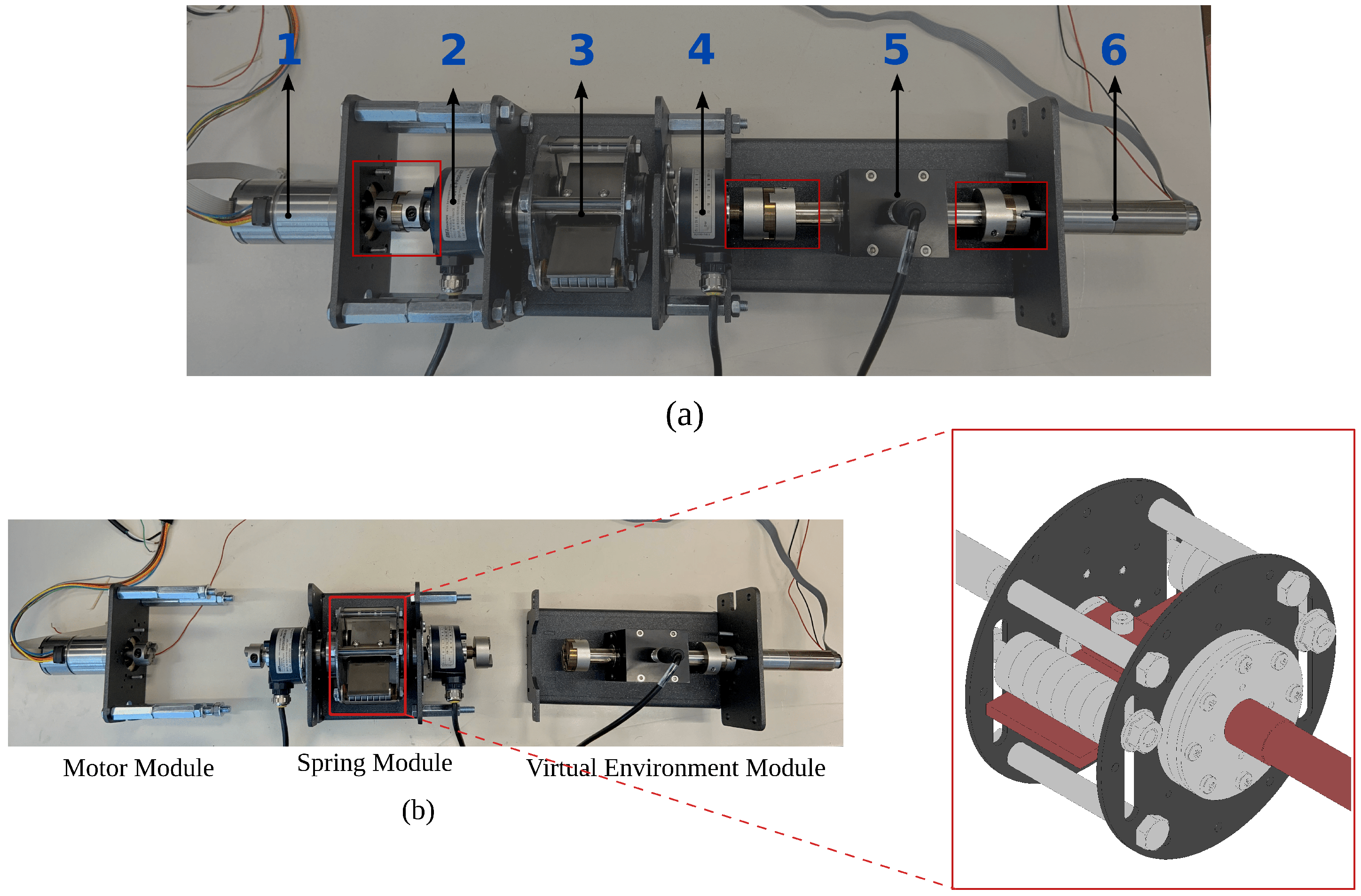
The mechanical structure of the affordable Forecast Testbed has been realized with laser-cut and welded iron layers. To combine sensors and actuators with different rotation shaft diameters we used Oldham couplers which allowed us to re-arrange the modules maximizing the modularity. A picture of the Forecast testbed is shown in Figure 1, where (1) is main the actuator, (2) the actuator encoder, (3) a series spring, (4) the environment encoder, (5) the torque sensor, (6) the VEM. The spring module is based on harmonic steel leaves with different thicknesses and different stiffness as a consequence. The user can compose leaves in order to achieve the desired torsional stiffness. A detailed CAD model of the spring module can be seen in Figure 1b. Testbed parameters are reported in Table 1.
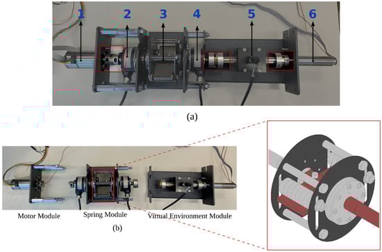
Figure 1.
Two pictures of the Forecast testbed where (a) represents the configuration of a Series Elastic Actuator (SEA). (b) highlights each module and emphasizes the easy-to-configure idea. Also, a detailed CAD view of the leaf spring mechanism within the spring module can be observed. The red parts are fixed to the motor shaft while the gray parts are fixed to the virtual environment module.

Table 1.
Forecast testbed parameters.
Mechanical inaccuracies are mainly due to shaft misalignments between different modules which lead to angle-dependent friction effects. In particular, in the testbed shown in Figure 1 we observed diverse stiction (i.e., static friction) magnitudes, diverse stick-slip dynamics (due to holdham joint sliding), and diverse Stribeck curves (due to lubricated bearings), depending on the initial position of the actuator.
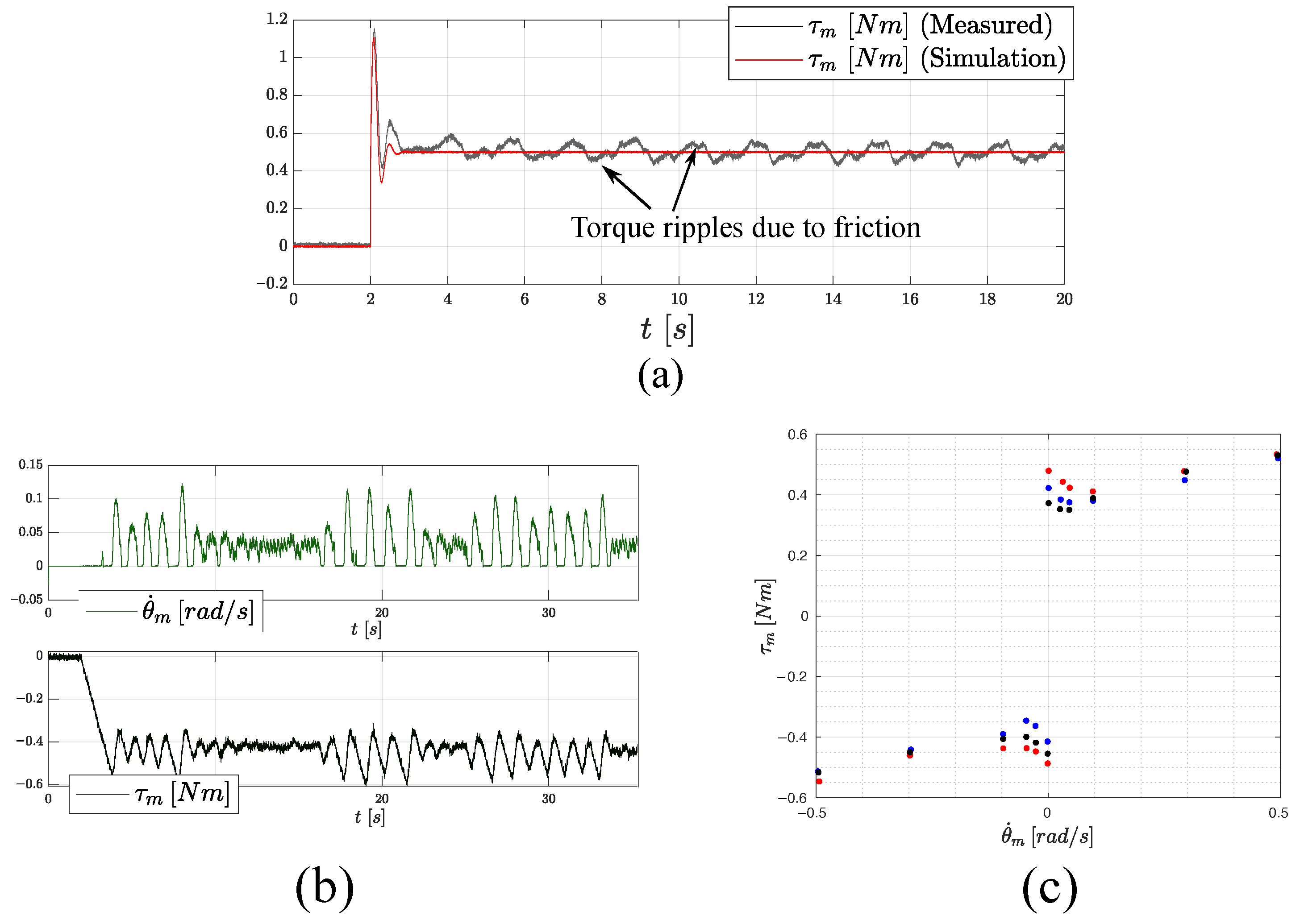
Figure 2a considers experimental and simulated actuator torques during a proportional-integrative () velocity control with P = 0.1 and I = 10. The values of P and I are manually adjusted to reach a stable and smooth control. By looking at the figure, the reader can observe periodic friction ripples on the measured motor torque . Figure 2b highlights how diverse and uncertain stick-slip phenomena significantly affect the actuator velocity () and torque (). Figure 2c reports three different friction identification experiments considering three different initial positions of the actuator to highlight the diverse stiction effects and Stribeck curves. Each dot in the figure comes from a single experiment and is obtained by averaging the measured velocity and torque values. For each of the three initial configurations, a total of 12 experiments were conducted (six experiments considering positive torques and velocities and six experiments considering negative torques and velocities). Each color corresponds to a set of experiments associated with a specific initial configuration. Data were collected in an open loop at zero velocity to improve the identification of the static friction and under the feedback action of a velocity control at low velocities to improve the identification of the Stribeck curve.
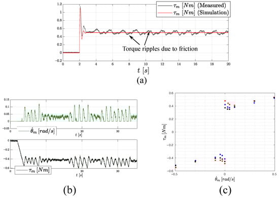
Figure 2.
Three pictures representing issues due to friction effects in the Forecast testbed shown in Figure 1. (a) shows simulated (red) and experimental (black) actuator torques during a velocity control, highlighting torque ripples due to friction. (b) shows that stick-slip effects affecting the testbed are extremely uncertain. (c) reports the outcome of three different friction identification procedures (each represented by a different color) highlighting different static friction magnitudes and different Stribeck curves.
By looking at the Figure it can be observed that different initial positions of the actuator lead to different friction profiles. In particular, different stiction effects and different Stribeck curves can be observed. Conversely, Coulomb and viscous friction profiles appear to be quite consistent regardless of the initial configuration of the motor.
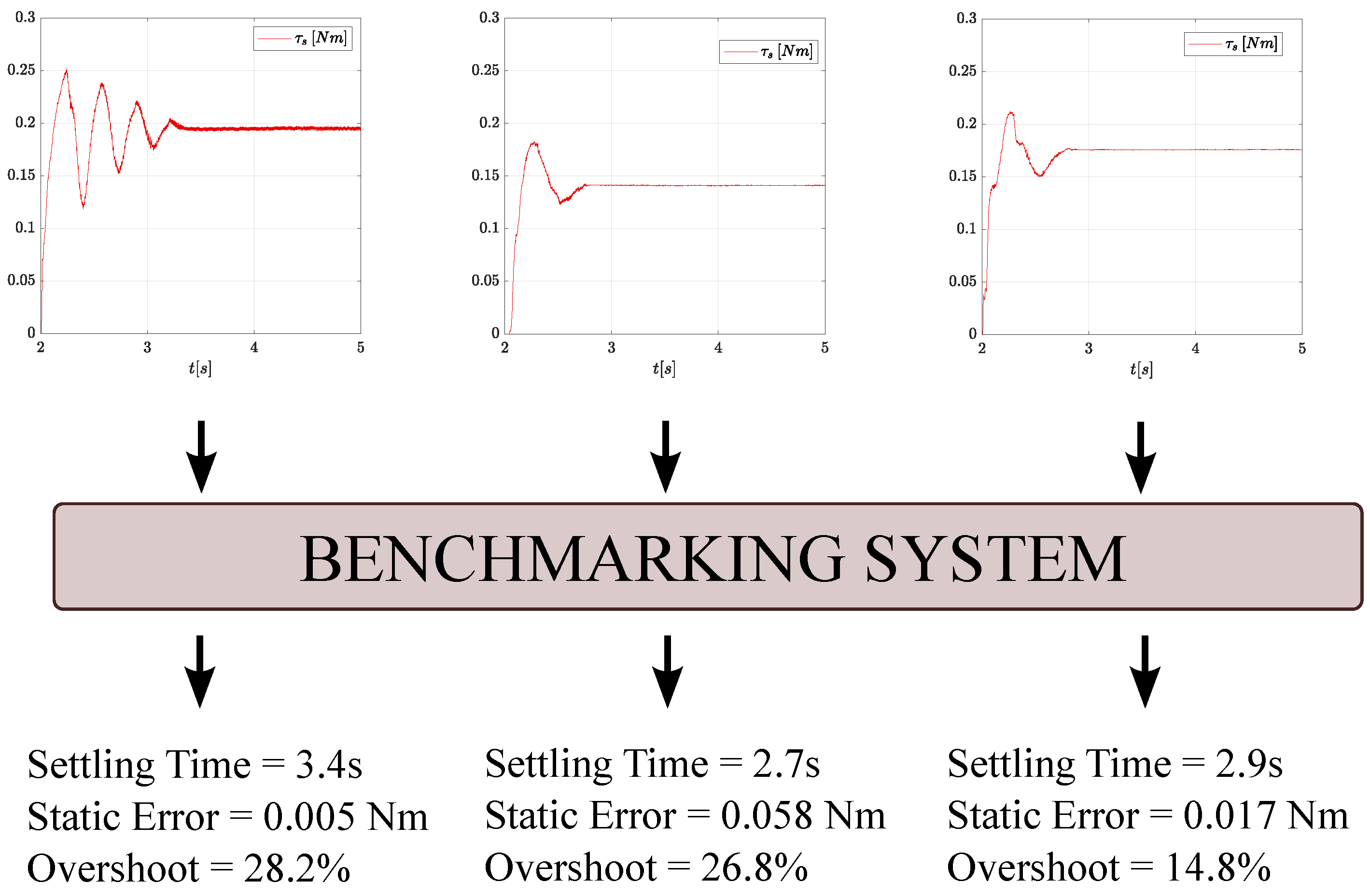
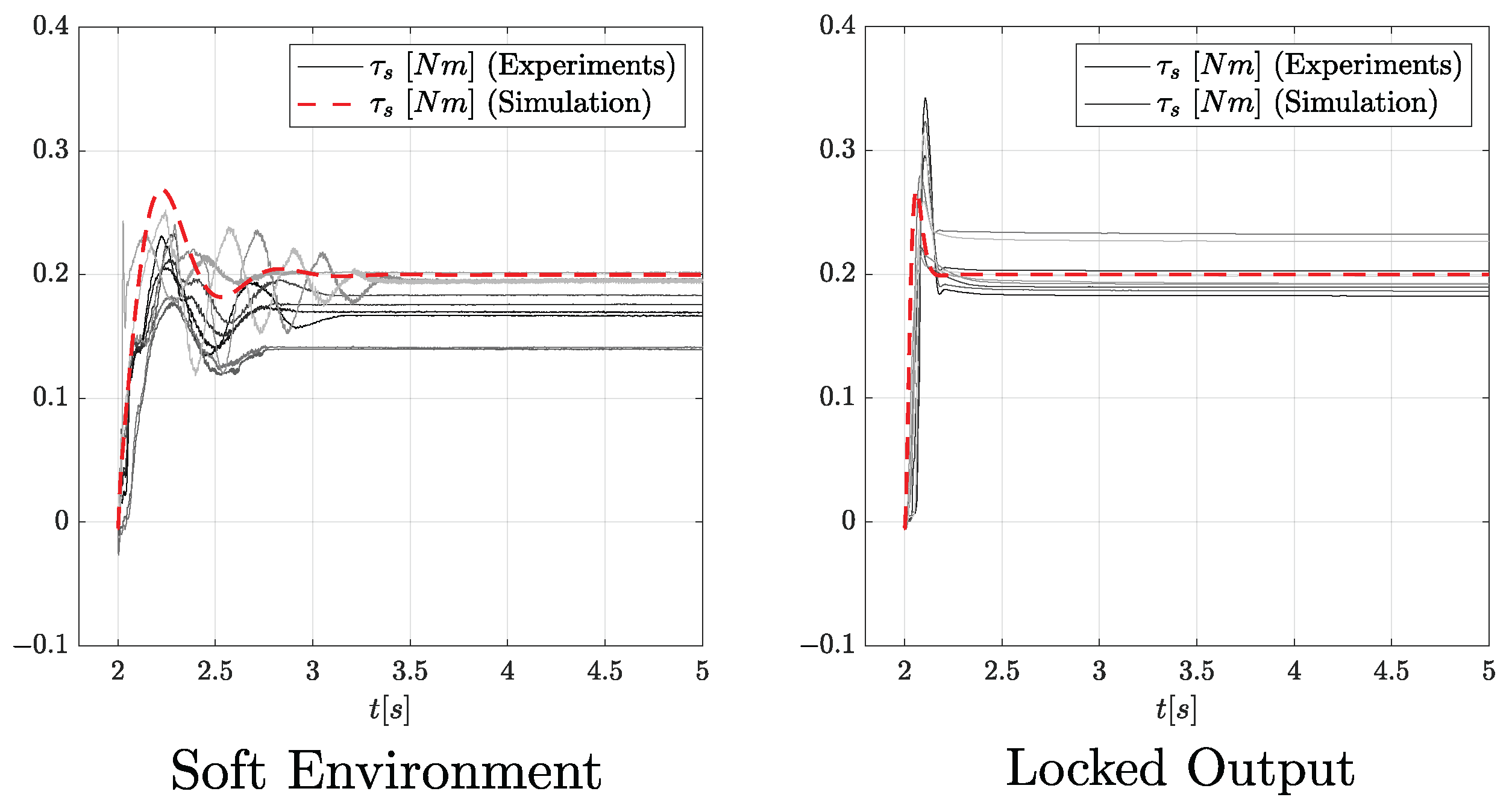
Such friction makes it hard to obtain accurate benchmarking because the testbed behaves quite differently between each test. This is shown in Figure 3, considering PD force control experiments in a soft interacting environment. The reader can notice how undesired friction effects lead to significantly different behaviors and, consequently, different benchmarking outcomes, despite the same control algorithm with the same tuning being applied.
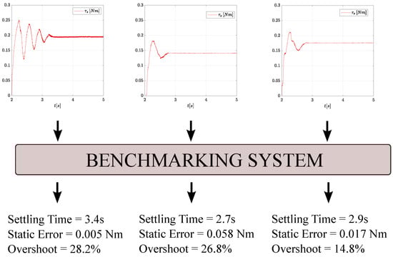
Figure 3.
A figure showing three experimental step responses of a PD force controller with the same tuning. Friction effects lead to significantly different benchmarking outcomes.
3. Background
3.1. Series Elastic Actuators (SEAs)
The modular Forecast testbed can be re-arranged allowing the designer to consider elastic or stiff actuator architectures. The SEA configuration is the one considered in this paper but similar considerations apply to the case of stiff actuators.
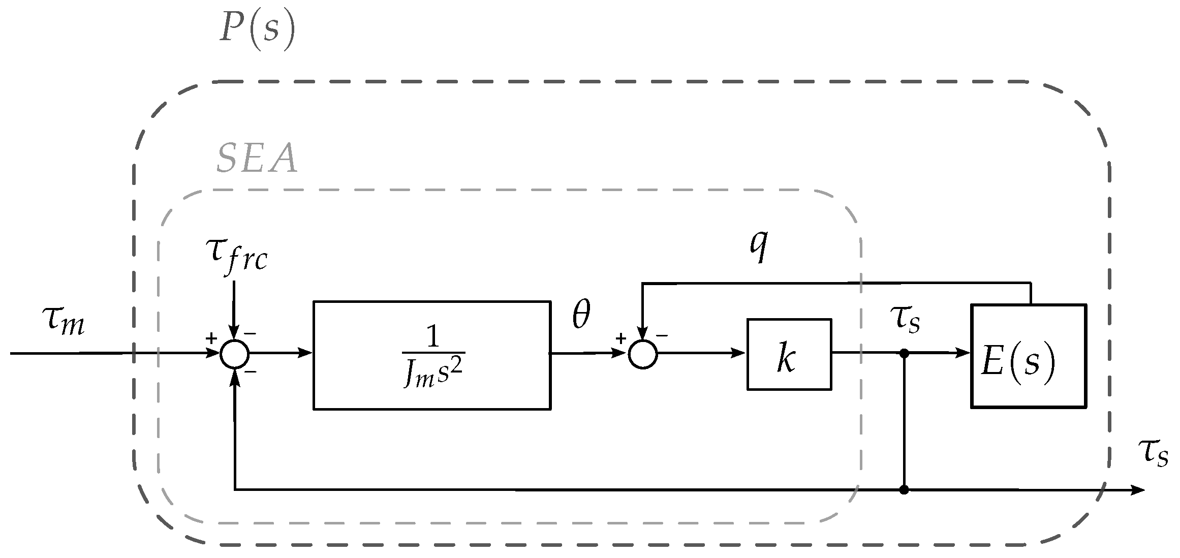
As represented in Figure 4, a SEA consists of a spring (having stiffness k) placed in series with a motor (having reflected inertia and viscous friction coefficient ). A SEA can be modeled with the following equations:
where is the motor position, q is the joint position, is the motor torque at the output shaft (which is proportional to the current and accounts for an eventual gear reduction), is the spring torque and represents friction torques. The interacting environment () is modeled as an inertia J (which may eventually include the robot link inertia coupled with the environment inertia , i.e., ), a damping d (which may eventually include the robot link damping coupled with the environment damping , i.e., ) and a stiffness . The plant dynamics (which explains the force dynamics between and ) can be derived as [1] where is linearized as :
where :
represents the environment dynamics (as rendered by the VEM).
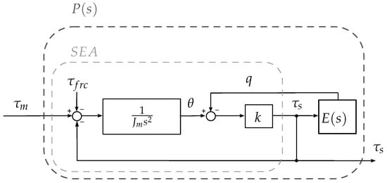
Figure 4.
Block diagram representation of a series elastic actuator interacting with a generic environment .
3.2. Friction Compensation
Friction compensation is an established topic in the literature. Many solutions have been proposed over the years and we report here only the most popular. Model-based friction compensation is a widespread strategy and the simplest friction model that can be adopted includes the Coulomb friction used in combination with viscous friction [12,13,14,15,16,17,18,28]. In the paper we refer to this model as the Simple Friction Model, i.e., SFM. In this case, friction parameters are identified offline and friction compensation is performed through a feed-forward action. However, since friction parameters are temperature-variant and time-variant, SFM compensation may be inaccurate. Higher accuracies can be achieved by exploiting adaptive strategies [19,20,21,22]. Nevertheless, such adaptive approaches are suitable only for position (or velocity) control and not in the case of force control. Friction observers (FOBs) represent another effective approach [15,24,29,30], but again existing FOB are suitable only for position or velocity-controlled systems. An example is the FOB designed to compensate for joint friction effects in the DLR robot arms [15]. More generally, if we consider existing DOBs applied to force control, the interacting environment is always treated as a disturbance, and thus, the DOB action rejects both disturbances due to friction and to the environment without clearly distinguishing them. Alternative solutions to standard DOBs consider the so-called reaction torque/force observer (RTOB/RFOB). These approaches can distinguish between friction forces and environmental forces but just for torque estimation purposes and not for friction compensation [16].
In conclusion, FOBs do not exist for force control applications and only model-based approaches are suitable for a force control benchmarking application. In fact, these strategies do not cancel or alter the effects of the interacting environment, ensuring reliable benchmarking.
Given these premises, this paper proposes a novel approach; the details are discussed in the next Section.
4. Environment Aware Friction Observer
Generally speaking, DOB-based force controllers aim to enforce a nominal model to the force dynamics despite environment uncertainties and unmodelled disturbances. DOB-based force control of SEAs is an established research topic [7,13,25,26,31]. Different solutions have been proposed which can be classified as:
- Open-loop DOBs [13,32], where disturbance rejection is applied exclusively to the plant dynamics,
- Closed-loop DOBs [26,33], which aim to reject disturbances on the entire closed-loop force dynamics.
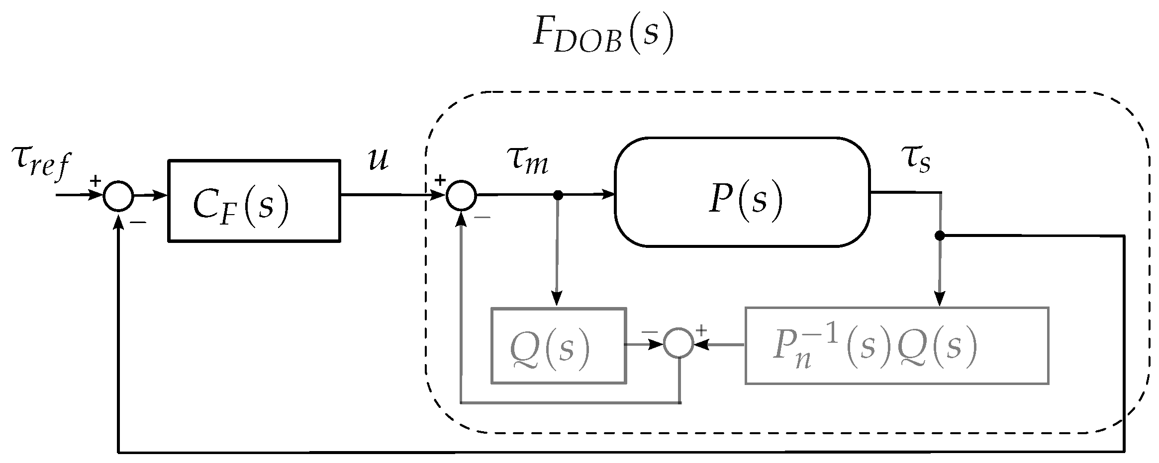
SinceRoozing et al. have recognized the equivalence between these two DOB architectures [34], this paper focuses solely on the open-loop (OL) configuration shown in Figure 5. In this case, the force dynamics between u (i.e., the output of the force controller) and is expressed as:
Within the Forecast framework, we are aware of the environment dynamics at every step of the benchmarking process (i.e., parameters , and are known). This allows us to consider a novel DOB architecture that we call environment-aware friction observer (EA-FOB). Since the EA-FOB is designed to compensate friction, the nominal plant recalls the one expressed in (3) while excluding the term :
Different from existing DOB solutions, the environment is no longer treated as an unknown disturbance to be rejected but becomes an integral part of the nominal plant. This leads the EA-FOB action to reject disturbances due to mechanical friction effects. For this reason, in this paper, we propose to use the EA-FOB as an inner loop during the benchmarking process with the specific objective of rejecting disturbance only due to friction.

Figure 5.
A block diagram of the considered DOB force control architecture, where is a generic force controller, represents the nominal model and is a low-pass filter used to both allow the nominal model inversion and to tune the frequency () up to which disturbances are rejected. The dynamics of is expressed as (2).
In the following sections, we show how existing DOB solutions are related to the proposed EA-FOB and how the latter does not alter the inherent stability properties of the system. The same does not hold for other existing DOB architectures.
4.1. Relations with DOB-Based Force Control for SEAs
Existing OL-DOBs solutions assume the following nominal plants .
4.1.1. Nominal Plant with Locked-Output (LO-DOB)
In [32], Hopkins et al. proposed an open-loop DOB architecture to enforce the force dynamics of a series elastic humanoid to the sole locked-output actuator dynamics. This leads such DOBs to reject disturbances due to the humanoid frame dynamics, unmodelled friction effects and time-varying interacting environment. In practice, the considered nominal model describes the interaction with an infinitely stiff environment, i.e., a locked-output system configuration. Such approximation can be formally expressed as a special case of our nominal model (5) where the environment stiffness is infinite:
4.1.2. Nominal Plant with Link Dynamics (LD-DOB)
Oh et al. recently proposed using a two-mass SEA nominal model that neglects the interaction forces with the environment but includes the link dynamics [31,35]. This case is equivalent to considering:
in Equation (5), where represents the link inertia and is the link damping. Therefore, the nominal plant can be expressed as:
Thus, both the LO-DOB and LD-DOB are particular cases of the EA-FOB. The reader can indeed observe how (6) and (8) just consider a “partial” in (5).
Although the friction compensation capabilities of such DOB solutions have been proven to be effective [25,26,32,35,36], it is important to state that they cannot be exploited within the Forecast project as they lead to the rejection of the environment dynamics too. Since the Forecast project needs to evaluate force algorithm performance when interacting with different environments, the proposed EA-FOB is able to accurately compensate only friction effects without altering the environment dynamics, thus ensuring proper benchmarking.
5. Stability Robustness Analysis
In this Section, we show that differently from the LO-DOB and the LD-DOB, the proposed EA-FOB does not significantly alter the inherent stability of the system and thus, guarantees a non-biased benchmarking process. The reason behind this comparison is that in many practical cases, DOBs may heavily alter the closed-loop stability. This happens because the DOB nominal model may be significantly different from the system dynamics and this leads to lower stability margins. In these cases, an aggressive filter is needed to mitigate such model mismatch and to guarantee closed-loop stability [37,38,39]. However, using a slow filter may lead to some disadvantages, including the inability to reject high-frequency friction disturbances such as stiction and stick-slip effects. This requires redesigning the filter to find a reasonable trade-off between performance and stability robustness [40]. The focus of this section is to showcase that the EA-FOB can tolerate a reasonably high frequency filter while showing higher stability margins, despite environment uncertainties, with respect to other existing DOB-based force control approaches. As mentioned before, other DOBs are not suitable for our purpose since they cannot isolate friction effects, and they are considered here only for stability comparison purposes.
Although gain and phase margin represent classical approaches to determining the stability and robustness of a system, they suffer from some limitations. Even if both magnitude and phase affect system stability, simultaneous magnitude and phase perturbations are not captured by classical margins. As a consequence, small simultaneous plant perturbations may cause stability issues even if the system has high gain and high phase margins [41]. For this reason, we adopt a recently proposed approach called disk margins (DM) [41]. Disk margins are robust stability measures that account for simultaneous gain and phase perturbations.
Let us define f as a complex-valued multiplicative factor describing simultaneous gain and phase perturbations of an open-loop system . In extremely simple words, DM defines the largest circular area D which encloses all the complex perturbations f such that closed-loop with is well-posed and stable. Even if disk margins represent a more comprehensive approach than classical margins they are still conservative as they account only for a circular sub-area of the perturbation space. An in-depth analysis of DM is out of the scope of this paper, for further details see [41].
Stability Robustness Comparison
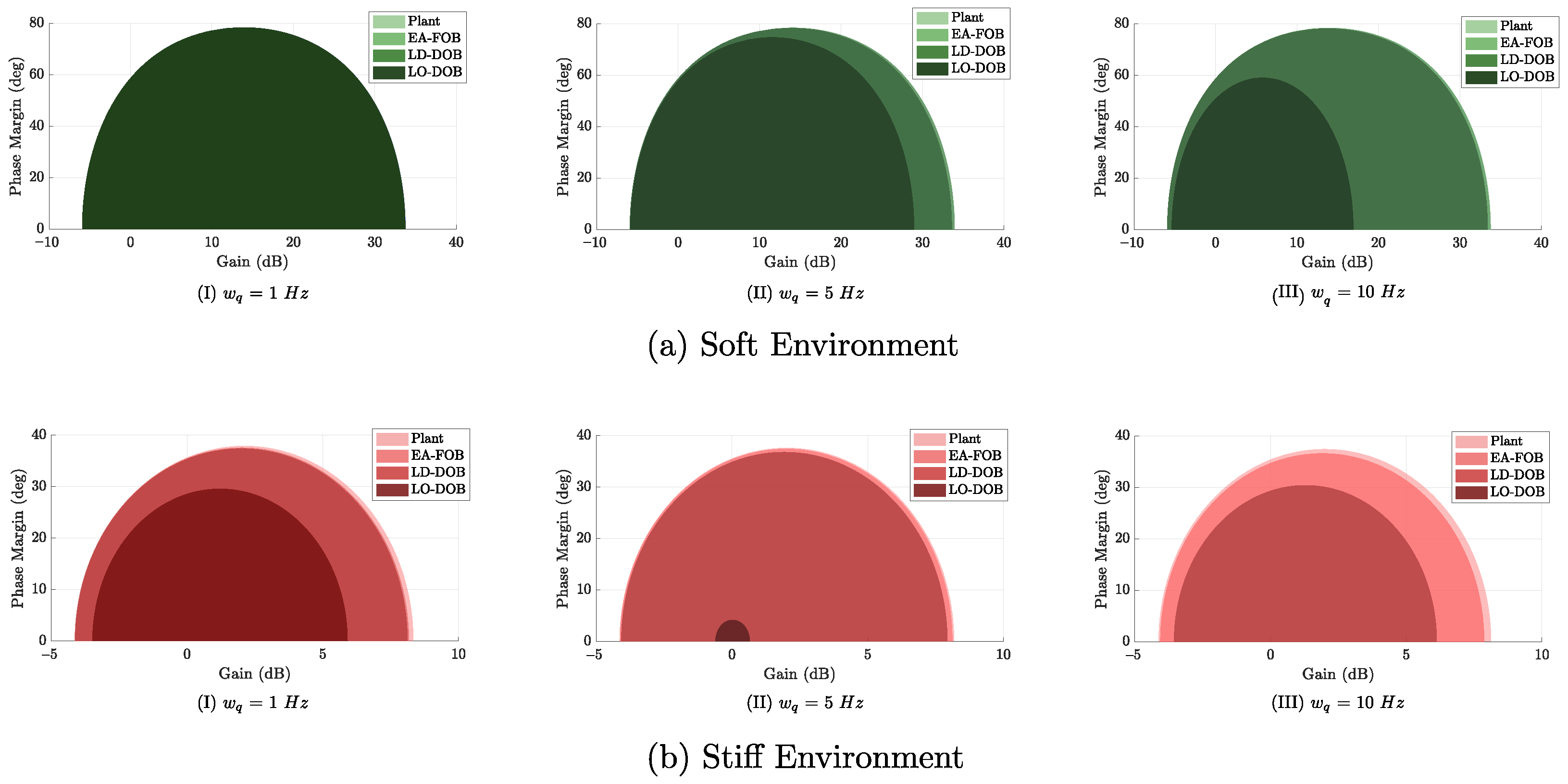
In this subsection, we use DMs to assess the robustness of the proposed EA-FOB. Stability robustness is assessed considering a soft interacting environment expressed as , , and a stiff interacting environment expressed as , . The value of is set to reach a critically damped environment. We accounted also for the link dynamics, modeled as a rigid body having inertia and damping , and coupled with the environment (i.e., , ). The cutoff frequency of the DOB filter is set to 1 Hz, 5 Hz and 10 Hz, respectively. DM results are shown in Figure 6. Since the disk area is mirrored with respect to the real axis, in this paper we will adopt a more compact representation considering only the upper half-disk representation.
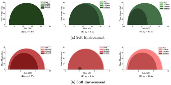
Figure 6.
Disk margins of the considered DOB solutions.
Figure 6a shows DMs for the case of a soft environment where the main interacting dynamics are given by the link. Since the considered scenario resembles the LD-DOB nominal plant (8), the LD-DOB achieves higher stability margins while the LO-DOB significantly deteriorates the inherent plant stability as the frequency increases. On the other hand, Figure 6b shows DMs in the case of a stiff interacting environment. In this case, the reader can observe higher stability margins for the LO-DOB. This is expected since such a DOB considers a nominal plant interacting with an infinitely stiff environment. Conversely, the LD-DOB deteriorates the inherent plant stability, leading even to an unstable behavior for (as indicated by the disappearance of the dark red disk). The EA-FOB always shows higher stability margins extremely close to the plant itself regardless of the environment, outperforming the other solutions. The very small difference between the DM of EA-FOB and the plant itself (particularly highlighted when Hz) is due to the friction parameter which is set to zero in the nominal plant. This represents a worst-case condition (since an estimation of can be easily obtained in practice) where the the EA-FOB is enforced to fully compensate for friction forces. Nevertheless, as observed before, the stability margins of the EA-FOB remain extremely close to those of the original plant. Such impressive stability and robustness can be explained by considering that the EA-FOB nominal plant is always close to the real one. Differently, the other DOB solutions consider approximated or partial models for the environment which lead to larger deviations from the real plant.
6. Simulation Results
This section compares the friction compensation accuracy of the EA-FOB with that of an SFM in a simulated environment. The real-world friction affecting the actuator dynamics is simulated considering the LuGre model [24]. This model allows us to account for both static and dynamic friction effects, showcasing the EA-FOB capabilities to accurately observe them. The parameters reported in Table 2 are chosen for simulation purposes only.
Table 2.
Friction parameters of the simulated LuGre model.
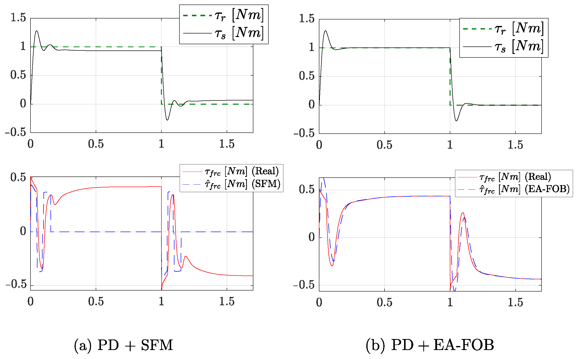
Simulations are carried out in Matlab considering the block diagram shown in Figure 5, where is a simple controller tuned to provide a control bandwidth around 10 Hz when interacting with a high-impedance environment (, = ). This leads to and . Simulation results are shown in Figure 7. The left side shows the results of SFM compensation while the right side shows the results of the EA-FOB compensation. The upper plots show the torque tracking performance, where is a square wave (drawn in gray) and is the spring torque (drawn in black). In the lower plots, (drawn in red) represents the simulated friction torque while (blue dashed line) represents the estimated friction torque. In the case of SFM, is defined as:
where and represent the viscous and the Coulomb friction parameters, respectively. In the case of EA-FOB, is defined as:
where is the EA-FOB nominal plant defined in (5) while the cutoff frequency of the filter is set to 10 Hz.
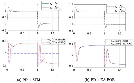
Figure 7.
Simulation results considering a SFM friction compensation and the proposed EA-FOB friction compensation.
By looking at the plots, one can observe that the proposed EA-FOB exhibits a superior accuracy in observing friction with respect to an SFM. Indeed, the mean absolute error (MAE) between and is Nm in the case of SFM and Nm in the case of EA-FOB. Moreover, it can be clearly seen that the EA-FOB compensates for disturbances due to friction while ignoring other disturbances, e.g., due to the interacting environment.
7. Experimental Results
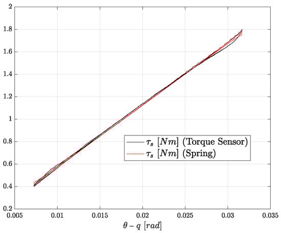
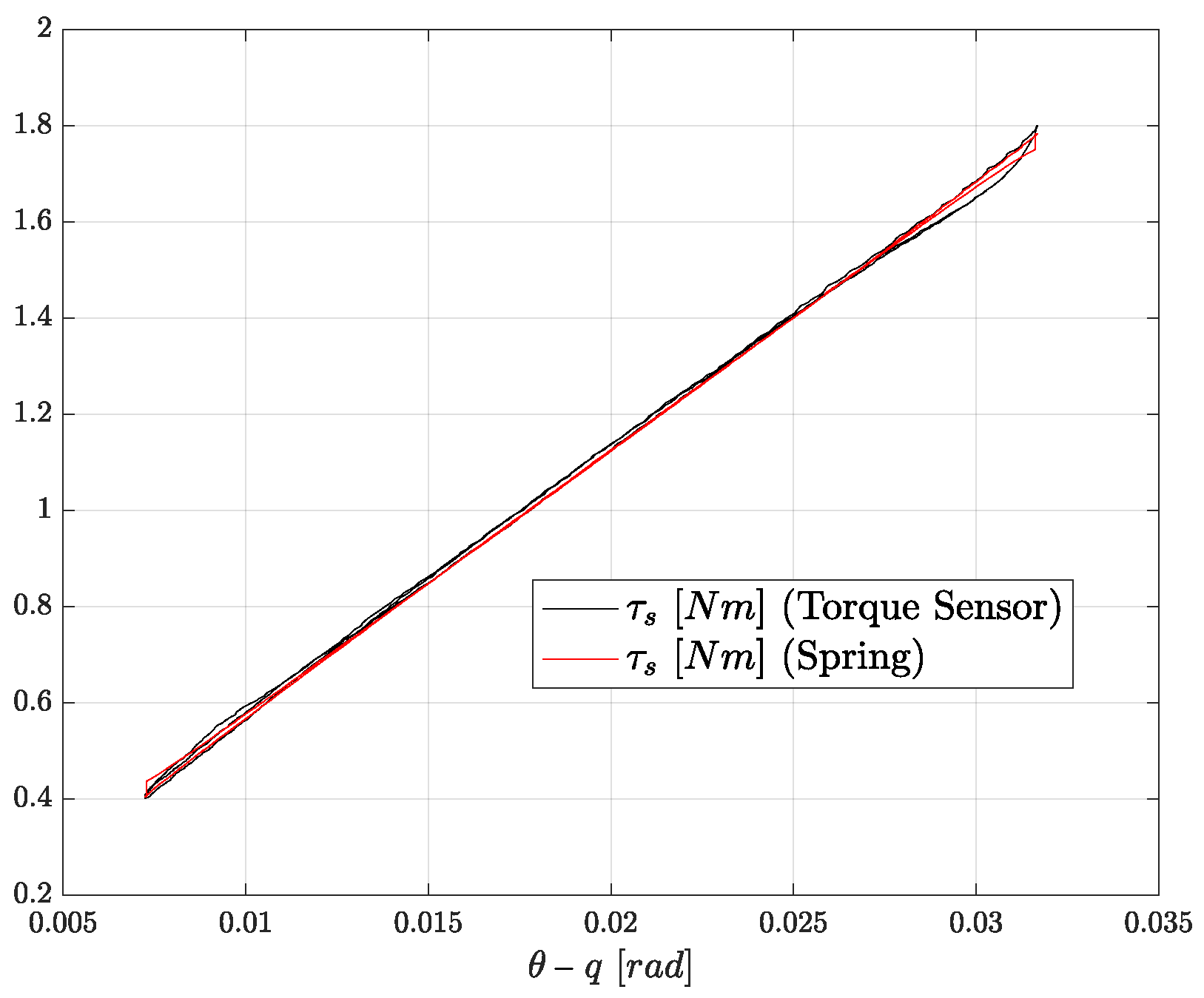
The objective of the experiments is to evaluate the friction compensation capabilities of the proposed EA-FOB and to validate the stability considerations reported in Section 5. Experiments are carried out using the Forecast testbed shown in Figure 1. In this setup, motors are driven in current control mode using a commercial driver (ESCON 50/5) while the force control algorithms run on an embedded board (Nucleo F446RE) as a periodic hard real-time process with a frequency of 2 kHz. Two optical encoders (DHO-05) with an extremely high resolution (2,000,000 pulses per revolution) are used to measure the motor position and the environment position q. The feedback torque is measured using spring deflection according to (1). Such spring has a linear stiffness profile and negligible inherent friction, as shown in Figure 8.
To experimentally evaluate the friction compensation capabilities of the proposed EA-FOB, we evaluate how much the undesired friction effects affecting the Forecast testbed can be reduced. A comparison with SFM compensation is carried out. It is important to specify that only Coulomb and viscous friction can be conveniently compensated as they exhibit invariant dynamics. Conversely, stick-slip phenomena, static friction effects and Stribeck curves are extremely uncertain, as shown in Figure 2.
In optimal conditions, the force control response should be repeatable and not influenced by variabilities due to friction effects. Thus, the objective of the experiments is to measure the repeatability of ten step responses. Each experiment considers the same control tuning and the same interacting environment. Since the mechanical friction of our testbed depends not only on the velocity , but also on the angle with periodic trends, we considered an extended SFM which includes sine and cosine functions based on the actuator angle. Friction parameters are identified by exploiting a least squares approach and the estimated friction torque can be formally defined as:
where P is the vector of friction parameters and is defined as:
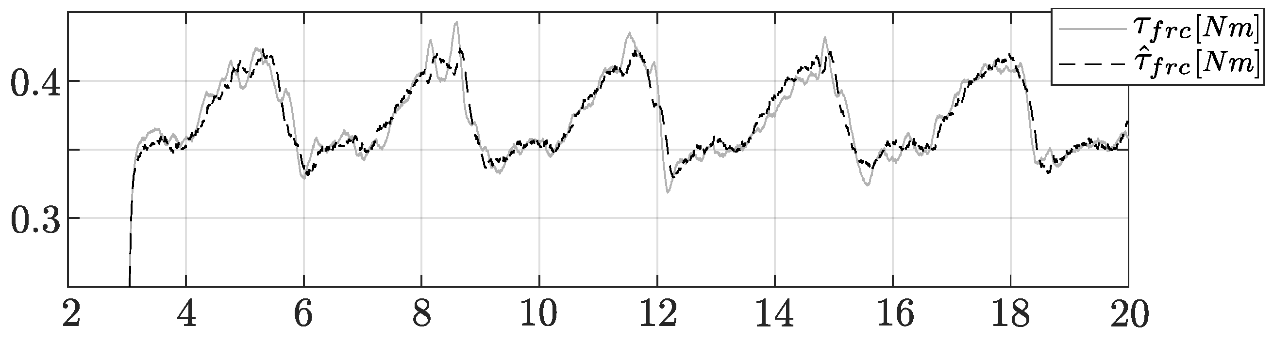
where the sine and cosine functions are shortened as s and c, respectively. Friction identification results are shown in Figure 9 where is the measured friction torque. The fitting accuracy achieved is 89.95%.

Figure 9.
Extended SFM friction identification outcomes.
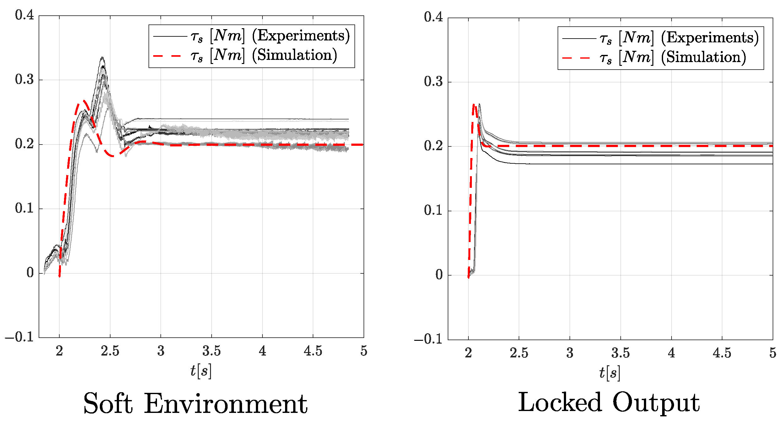
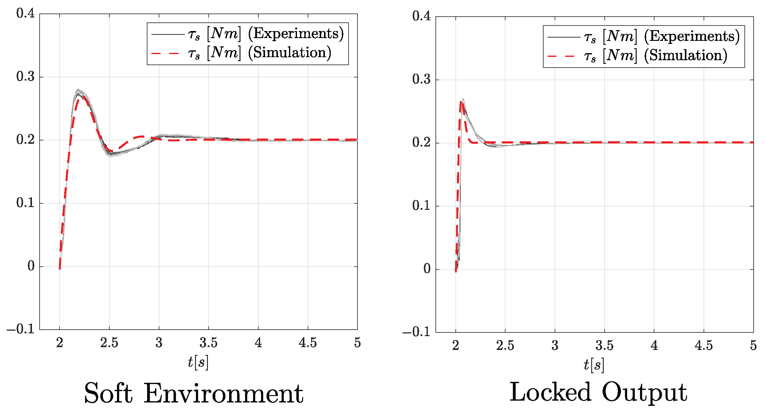
The main experimental results are reported in Figure 10, Figure 11 and Figure 12, showing for each plot the repeatability of the ten step responses. Figure 10 considers a PD control without any friction compensation, Figure 11 considers a PD with SFM friction compensation and Figure 12 considers a PD with EA-FOB friction compensation. In each Figure, the left plot refers to a soft environment interaction ( = 0.001 and = 5 ) while the right plot refers to a locked-output configuration, specifically chosen to represent the scenario with the highest possible environment stiffness. All the experiments consider a desired step reference. The same PD controller used in the simulation is considered (P = 5 and D = 0.1). The frequency of the EA-FOB is again set to 10 Hz.
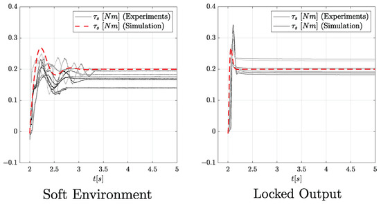
Figure 10.
Step responses considering the PD force controller without any friction compensation law. The red dashed line simulates how the system would perform under the control action of the PD in the absence of friction.
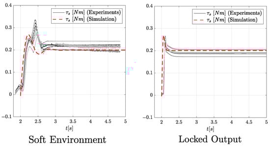
Figure 11.
Step responses considering the PD force control with an SFM compensation. The red dashed line simulates how the system would perform under the control action of the PD in the absence of friction.
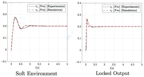
Figure 12.
Step responses considering the PD force control with the proposed EA-FOB algorithm. The red dashed line simulates how the system would perform under the control action of the PD in the absence of friction.
Looking at the PD responses one can observe how, without any friction compensation law, undesired friction effects critically affect the control responses leading to not repeatable behaviours.
A significant improvement can be seen by exploiting an SFM. In this case, responses look more repeatable even though undesired low-frequency oscillations and high-frequency vibrations negatively affect the performance in the soft environment case and different static errors can be observed in the locked-output case. The EA-FOB is the only solution exhibiting smooth and repeatable responses when interacting with both soft and stiff environments characterized by low static errors. Quantitatively, friction compensation capabilities are assessed by considering two metrics: the repeatability of the control responses and the mean absolute error (MAE) between the experimental and expected responses.
The repeatability of control responses is assessed by computing the mean cross-correlation among step responses of different experiment repetitions. Mean cross-correlation values are reported in Table 3, showing that the EA-FOB and the SFM exhibit high cross-correlation indices, highlighting the repeatability of responses. Although cross-correlation is effective for measuring repeatability it does not provide sufficient insights into the friction compensation performance. For this reason, we decided to simulate how the system would perform in the absence of friction and calculate the MAE between these expected responses and the experimental ones. The expected responses are drawn as red dashed lines in Figure 10, Figure 11 and Figure 12, while MAEs are reported in Table 3. By looking at the plots, it is evident that the EA-FOB responses are closer to the simulated ones. The same does not hold for the SFM. For example, the reader may observe a slight delay between the actual and the expected response in both the stiff and soft case which is probably due to static friction. In conclusion, the metrics in Table 3 show the superior friction compensation capabilities of the EA-FOB which guarantees higher repeatability and higher fidelity responses.
Table 3.
Metrics used to quantitatively assess the friction compensation capabilities.
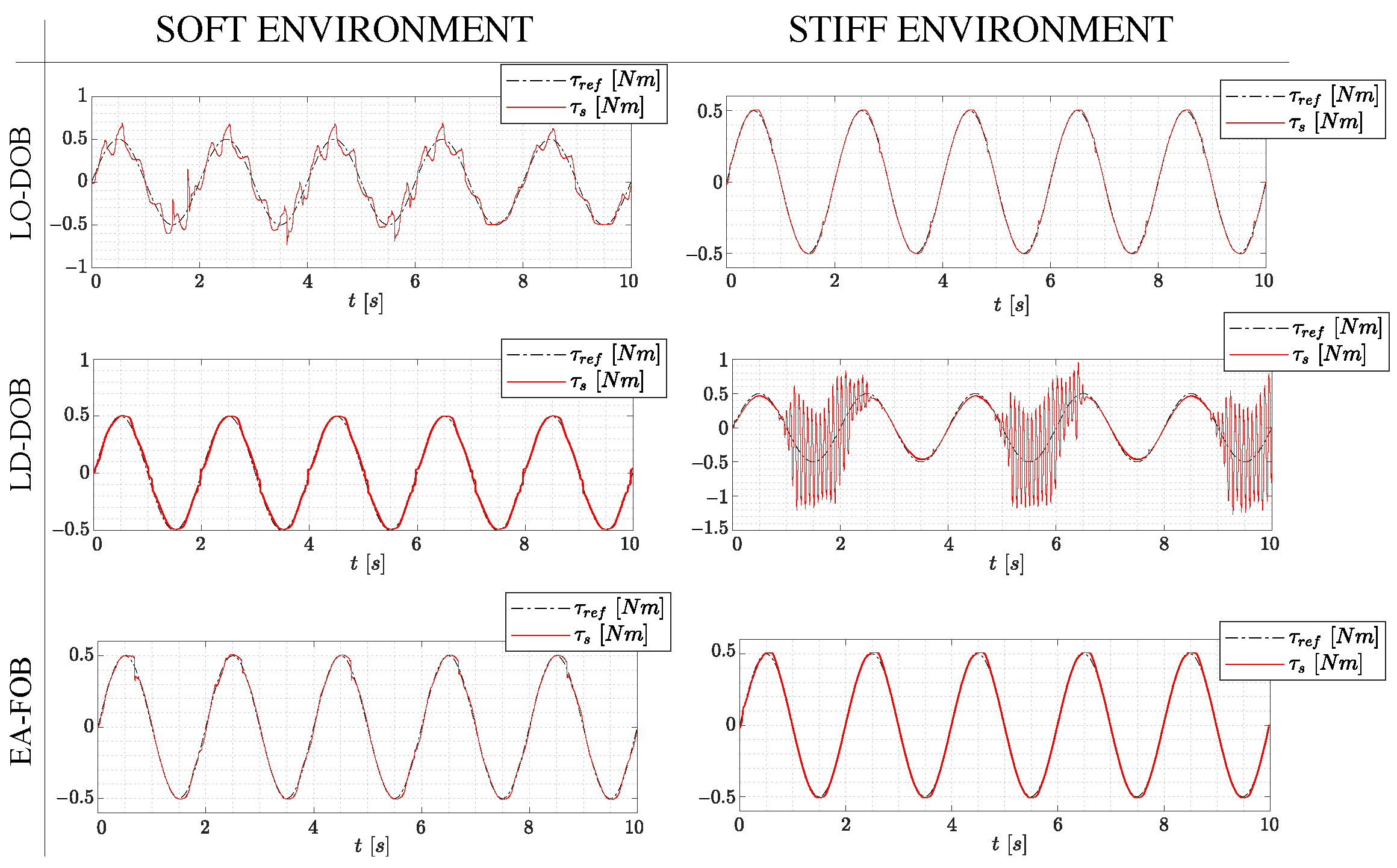
To assess the superior stability robustness of the EA-FOB with respect to an LO-DOB and LD-DOB, six different torque tracking experiments are conducted. Experiments consider a 0.5 Hz sinusoidal reference and the interaction with a soft and stiff environment. The tuning frequency of the filter is set to 10 Hz for all DOBs. Control responses are reported in Figure 13. In the case of a soft interacting environment, the LO-DOB response leads to undesired low-frequency oscillations. This reveals the presence of a complex conjugated pole pair which is related to lower stability margins. Similarly, the LD-DOB presents high-frequency vibrations when interacting with the stiff environment which again, can be related to lower stability margins. Instead, in all the experiments the EA-FOB shows accurate and non-oscillatory responses which can be related to higher stability margins.
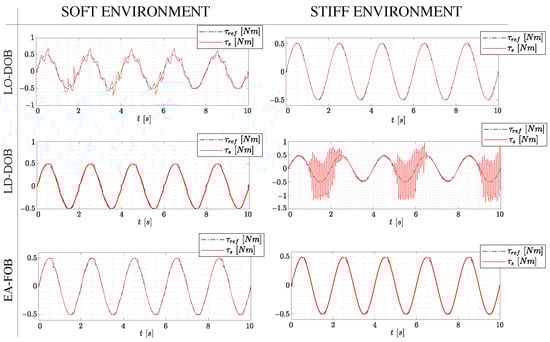
Figure 13.
Torque tracking of the considered DOB architectures interacting with a soft and a stiff environment. Each experiment is carried out with the same force controller tuned as P = 5 and D = 0.1.
In conclusion, these experimental results seem to confirm the disk margin analysis proposed in Section 5 with the EA-FOB showing better behaviors on the whole set of interacting environments.
8. Conclusions and Future Directions
Force control benchmarking needs to guarantee accurate and non-biased algorithm evaluations despite possible testbed mechanical issues. An affordable testbed may suffer from undesired friction effects which may jeopardize the algorithm assessment. However, affordability becomes of great help to spread benchmarking solutions among the research community. In this paper, we present a novel friction observer to accurately compensate for undesired mechanical friction effects affecting our affordable benchmarking testbed. A stability analysis based on DMs is reported, showing that the proposed EA-FOB does not deteriorate the inherent plant stability. EA-FOB friction compensation capabilities are assessed in simulation and experimentally, showing superior accuracy with respect to an SFM. Finally, since the proposed EA-FOB outperforms existing compensators, a meaningful future direction is to extend the use of EA-FOB outside of benchmarking applications where knowledge of the environment is usually missing or extremely imprecise. Unfortunately, the main limitation of the proposed approach is that it requires knowledge of the environment, otherwise it cannot be applied. Therefore, online estimation of environmental properties should be considered.
Author Contributions
Conceptualization, E.D. and A.C.; Methodology, E.D. and A.C.; Software, E.D.; Validation, E.D.; Formal analysis, E.D. and A.C.; Investigation, E.D.; Data curation, E.D.; Writing—original draft, E.D.; Writing—review & editing, E.D. and A.C.; Visualization, E.D. and A.C.; Supervision, A.C.; Project administration, A.C. Funding acquisition, A.C. All authors have read and agreed to the published version of the manuscript.
Funding
This research has been funded by the European Union’s Horizon 2020 program under grant agreement EUROBENCH n.779963.
Data Availability Statement
The data presented in this study are available on request from the corresponding author.
Conflicts of Interest
The authors declare no conflictS of interest. The founders had no role in the design of the study; in the collection, analysis, or interpretation of data; in the writing of the manuscript; or in the decision to publish the results.
References
- Calanca, A.; Fiorini, P. A Rationale for Acceleration Feedback in Force Control of Series Elastic Actuators. IEEE Trans. Robot. 2018, 34, 48–61. [Google Scholar] [CrossRef]
- Calanca, A.; Fiorini, P. Understanding Environment-Adaptive Force Control of Series Elastic Actuators. IEEE/ASME Trans. Mechatron. 2018, 23, 413–423. [Google Scholar] [CrossRef]
- Calanca, A.; Dimo, E.; Palazzi, E.; Luzi, L. Enhancing Force Controllability by Mechanics in Exoskeleton Design. Mechatronics 2022, 86, 102867. [Google Scholar] [CrossRef]
- Vicario, R.; Calanca, A.; Dimo, E.; Murr, N.; Meneghetti, M.; Ferro, R.; Sartori, E.; Boaventura, T. Benchmarking Force Control Algorithms. In Proceedings of the 14th PErvasive Technologies Related to Assistive Environments Conference, Corfu, Greece, 29 June–2 July 2021; Association for Computing Machinery: New York, NY, USA, 2021; Volume 1, pp. 359–364. [Google Scholar] [CrossRef]
- Behrens, R.; Belov, A.; Poggendorf, M.; Penzlin, F.; Hanses, M.; Jantz, E.; Elkmann, N. Performance Indicator for Benchmarking Force-Controlled Robots. In Proceedings of the 2018 IEEE International Conference on Robotics and Automation (ICRA), Brisbane, QLD, Australia, 21–25 May 2018; pp. 1653–1660. [Google Scholar] [CrossRef]
- Falco, J.; Norcross, R.; Norcross, R. Benchmarking Robot Force Control Capabilities: Experimental Results; NIST Interagency/Internal Reports (NISTIR) 8097; NIST: Gaithersburg, MD, USA, 2016.
- Ugurlu, B.; Sariyildiz, E.; Kansizoglu, A.T.; Ozcinar, E.; Coruk, S. Benchmarking Torque Control Strategies for a Torsion-Based Series Elastic Actuator. IEEE Robot. Autom. Mag. 2021, 29, 85–96. [Google Scholar] [CrossRef]
- Bruhm, H.; Czinki, A.; Lotz, M. High performance force control-A new approach and suggested benchmark tests. IFAC-PapersOnLine 2015, 28, 165–170. [Google Scholar] [CrossRef]
- Marvel, J.; Falco, J. Best Practices and Performance Metrics Using Force Control for Robotic Assembly; NIST: Gaithersburg, MD, USA, 2012. [Google Scholar]
- EUROBENCH2020. EUROpean Robotic Framework for Bipedal Locomotion bENCHmarking. Available online: https://cordis.europa.eu/project/id/779963 (accessed on 29 April 2023).
- Dimo, E.; Meneghetti, M.; Murr, N.; Calanca, A. The ForceCAST Framework: Methodology and Tools For Benchmarking Force Control Algorithms. Robot. Auton. Syst. 2023. to be submitted. [Google Scholar]
- Mahvash, M.; Okamura, A. Friction Compensation for Enhancing Transparency of a Teleoperator with Compliant Transmission. IEEE Trans. Robot. 2007, 23, 1240–1246. [Google Scholar] [CrossRef]
- Yu, H.; Huang, S.; Chen, G.; Pan, Y.; Guo, Z. Human-Robot Interaction Control of Rehabilitation Robots with Series Elastic Actuators. IEEE Trans. Robot. 2015, 31, 1089–1100. [Google Scholar] [CrossRef]
- Bernstein, N.L.; Lawrence, D.A.; Pao, L.Y. Friction modeling and compensation for haptic interfaces. In Proceedings of the 1st Joint Eurohaptics Conference and Symposium on Haptic Interfaces for Virtual Environment and Teleoperator Systems, World Haptics Conference, WHC 2005, Pisa, Italy, 18–20 March 2005; pp. 290–295. [Google Scholar] [CrossRef]
- Le Tien, L.; Albu-Schäffer, A.; De Luca, A. Friction observer and compensation for control of robots with joint torque measurement. In Proceedings of the IEEE/RSJ International Conference on Intelligent Robots and System, Nice, France, 22–26 September 2008; pp. 3789–3795. [Google Scholar]
- Sariyildiz, E.; Ohnishi, K. An adaptive reaction force observer design. IEEE/ASME Trans. Mechatron. 2015, 20, 750–760. [Google Scholar] [CrossRef]
- Toxiri, S.; Calanca, A.; Ortiz, J.; Fiorini, P.; Caldwell, D.G. A Parallel-Elastic Actuator for a Torque-Controlled Back-Support Exoskeleton. IEEE Robot. Autom. Lett. 2018, 3, 492–499. [Google Scholar] [CrossRef]
- Just, F.; Baur, K.; Riener, R.; Klamroth-Marganska, V.; Rauter, G. Online adaptive compensation of the ARMin Rehabilitation Robot. In Proceedings of the 2016 6th IEEE International Conference on Biomedical Robotics and Biomechatronics (BioRob), Singapore, 26–29 June 2016; pp. 747–752. [Google Scholar] [CrossRef]
- Lee, T.H.; Tan, K.K.; Huang, S. Adaptive Friction Compensation with a Dynamical Friction Model. IEEE/ASME Trans. Mechatron. 2011, 16, 133–140. [Google Scholar] [CrossRef]
- de Wit, C.C.; Lischinsky, P. Adaptive friction compensation with partially known dynamic friction model. Int. J. Adapt. Control Signal Process. 1997, 11, 65–80. [Google Scholar] [CrossRef]
- Huang, S.; Tan, K.; Lee, T. Adaptive friction compensation using neural network approximations. IEEE Trans. Syst. Man Cybern. Part C Appl. Rev. 2000, 30, 551–557. [Google Scholar] [CrossRef]
- Tan, Y.; Kanellakopoulos, I. Adaptive nonlinear friction compensation with parametric uncertainties. In Proceedings of the 1999 American Control Conference (Cat. No. 99CH36251), San Diego, CA, USA, 2–4 June 1999; Volume 4, pp. 2511–2515. [Google Scholar] [CrossRef]
- Roy, S.; Baldi, S.; Fridman, L.M. On adaptive sliding mode control without a priori bounded uncertainty. Automatica 2020, 111, 108650. [Google Scholar] [CrossRef]
- de Wit, C.C.; Olsson, H.; Astrom, K.; Lischinsky, P. A new model for control of systems with friction. IEEE Trans. Autom. Control 1995, 40, 419–425. [Google Scholar] [CrossRef]
- Kong, K.; Member, S.; Bae, J. Control of Rotary Series Elastic Actuator for Ideal Force-Mode Actuation in Human-Robot Interaction Applications. IEEE/ASME Trans. Mechatron. 2009, 14, 105–118. [Google Scholar] [CrossRef]
- Paine, N.; Mehling, J.S.; Holley, J.; Radford, N.A.; Johnson, G.; Fok, C.L.; Sentis, L. Actuator control for the NASA-JSC valkyrie humanoid robot: A decoupled dynamics approach for torque control of series elastic robots. J. Field Robot. 2015, 32, 378–396. [Google Scholar] [CrossRef]
- Calanca, A.; Muradore, R.; Fiorini, P. A Review of Algorithms for Compliant Control of Stiff and Fixed Compliance Robots. IEEE Trans. Mechatron. 2016, 21, 613–624. [Google Scholar] [CrossRef]
- Bona, B.; Indri, M. Friction compensation in robotics: An overview. In Proceedings of the 44th IEEE Conference on Decision and Control, Seville, Spain, 15 December 2005; Volume 2005, pp. 4360–4367. [Google Scholar] [CrossRef]
- Ruderman, M. Tracking control of motor drives using feedforward friction observer. IEEE Trans. Ind. Electron. 2014, 61, 3727–3735. [Google Scholar] [CrossRef]
- Lin, C.J.; Yau, H.T.; Tian, Y.C. Identification and compensation of nonlinear friction characteristics and precision control for a linear motor stage. IEEE/ASME Trans. Mechatron. 2013, 18, 1385–1396. [Google Scholar] [CrossRef]
- Asignacion, A.; Haninger, K.; Oh, S.; Lee, H. High-Stiffness Control of Series Elastic Actuators Using a Noise Reduction Disturbance Observer. IEEE Trans. Ind. Electron. 2022, 69, 8212–8219. [Google Scholar] [CrossRef]
- Hopkins, M.A.; Ressler, S.A.; Lahr, D.F.; Leonessa, A.; Hong, D.W. Embedded joint-space control of a series elastic humanoid. In Proceedings of the IEEE International Conference on Intelligent Robots and Systems, Hamburg, Germany, 28 September–2 October 2015; pp. 3358–3365. [Google Scholar] [CrossRef]
- Paine, N.; Oh, S.; Sentis, L. Design and control considerations for high-performance series elastic actuators. IEEE/ASME Trans. Mechatron. 2014, 19, 1080–1091. [Google Scholar] [CrossRef]
- Roozing, W.; Malzahn, J.; Caldwell, D.G.; Tsagarakis, N.G. Comparison of Open-Loop and Closed-Loop Disturbance Observers for Series Elastic Actuators. In Proceedings of the IEEE International Conference on Intelligent Robots and Systems, Daejeon, Republic of Korea, 9–14 October 2016; pp. 3842–3847. [Google Scholar]
- Oh, S.; Kong, K. High Precision Robust Force Control of a Series Elastic Actuator. IEEE/ASME Trans. Mechatron. 2017, 22, 71–80. [Google Scholar] [CrossRef]
- Just, F.; Özen, Ö.; Bösch, P.; Bobrovsky, H.; Klamroth-Marganska, V.; Riener, R.; Rauter, G. Exoskeleton transparency: Feed-forward compensation vs. disturbance observer. At-Automatisierungstechnik 2018, 66, 1014–1026. [Google Scholar] [CrossRef]
- Shim, H.; Jo, N.H. An almost necessary and sufficient condition for robust stability of closed-loop systems with disturbance observer. Automatica 2009, 45, 296–299. [Google Scholar] [CrossRef]
- Kong, K. Proxy-based impedance control of a cable-driven assistive system. Mechatronics 2013, 23, 147–153. [Google Scholar] [CrossRef]
- Schrijver, E.; Van Dijk, J. Disturbance observers for rigid mechanical systems: Equivalence, stability, and design. J. Dyn. Syst. Meas. Control 2002, 124, 539–548. [Google Scholar] [CrossRef]
- Choi, Y.; Yang, K.; Chung, W.K.; Kim, H.R.; Suh, I.H. On the robustness and performance of disturbance observers for second-order systems. IEEE Trans. Autom. Control 2003, 48, 315–320. [Google Scholar] [CrossRef]
- Seiler, P.; Packard, A.; Gahinet, P. An Introduction to Disk Margins [Lecture Notes]. IEEE Control Syst. Mag. 2020, 40, 78–95. [Google Scholar] [CrossRef]
Disclaimer/Publisher’s Note: The statements, opinions and data contained in all publications are solely those of the individual author(s) and contributor(s) and not of MDPI and/or the editor(s). MDPI and/or the editor(s) disclaim responsibility for any injury to people or property resulting from any ideas, methods, instructions or products referred to in the content. |
© 2024 by the authors. Licensee MDPI, Basel, Switzerland. This article is an open access article distributed under the terms and conditions of the Creative Commons Attribution (CC BY) license (https://creativecommons.org/licenses/by/4.0/).