
Practical System Identification and Incremental Control Design for a Subscale Fixed-Wing Aircraft


Abstract
1. Introduction
- Frequency domain identification of servo dynamics of different actuators both in flight and on ground using surface deflection measurements.
- Presentation of experimental results for system identification of a subscale fixed-wing aircraft using surface deflection measurements.
- Verification that the model resulting from system identification can accurately predict the closed-loop control law performance.
- Verification that iDPI control laws can obtain good performance on a subscale aircraft.
- Application of eigenstructure assignment for an iDPI lateral/directional control law.
- Derivation of kinematic relations for flow angle rates to avoid derivatives of load factor or flow angle measurements applicable to differential-integral control laws.
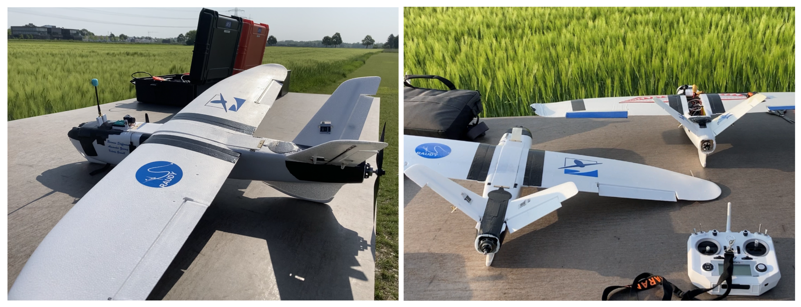
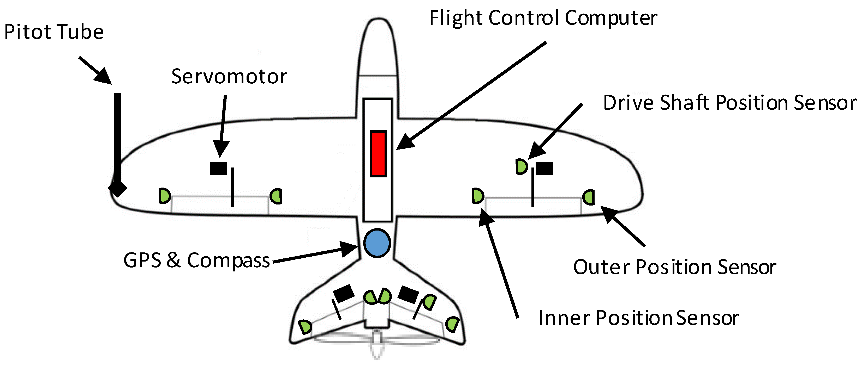
2. Experimental Setup
3. Identification of Servo+Surface Dynamics and Equivalent Time Delay
- Identify servo+surface transfer function models.
- Compare in-flight versus ground performance.
- Compare servo type, servo-surface linkage type and surface type.
3.1. Servo Motors
3.2. Excitation
3.3. Coherence
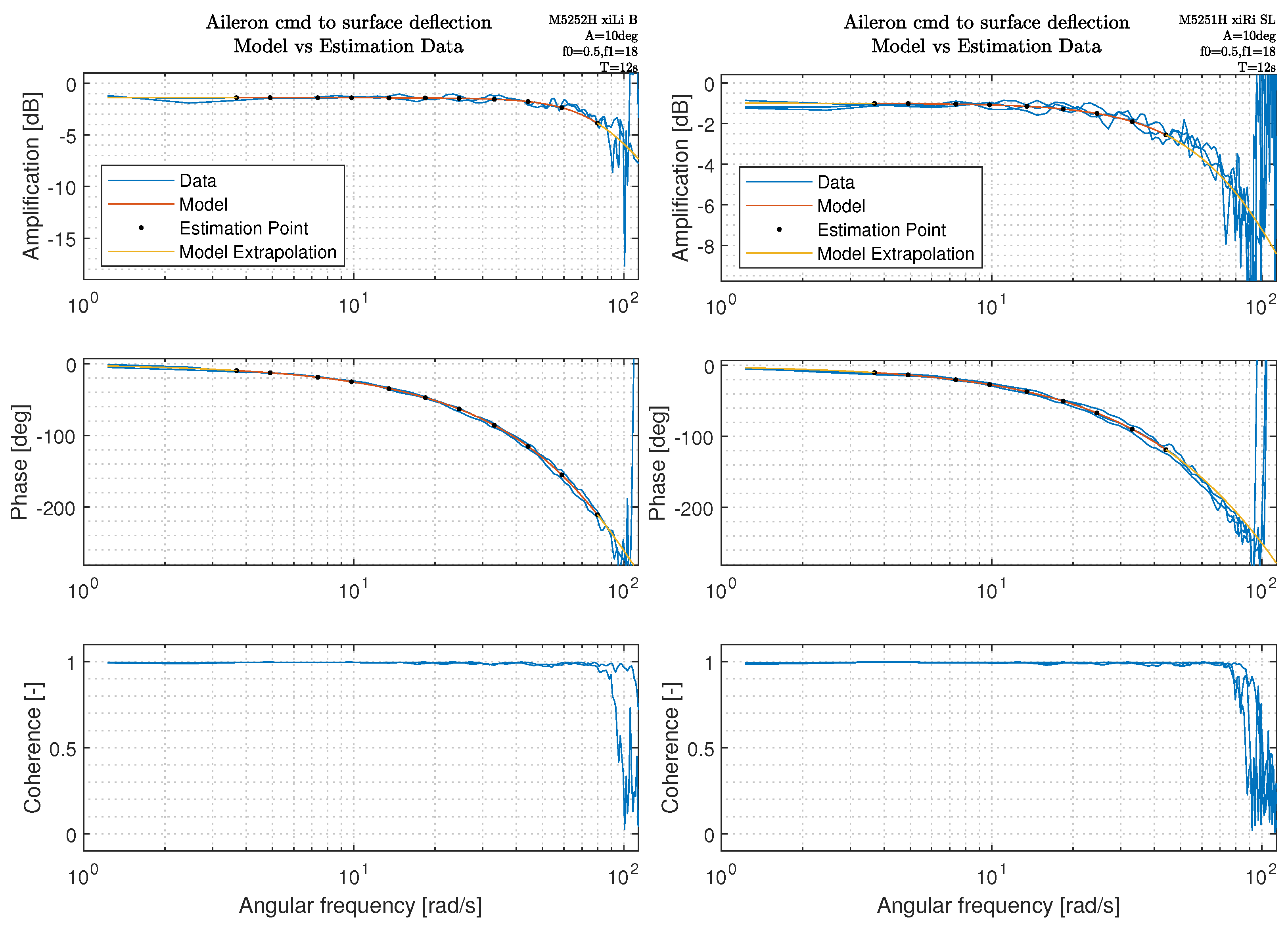
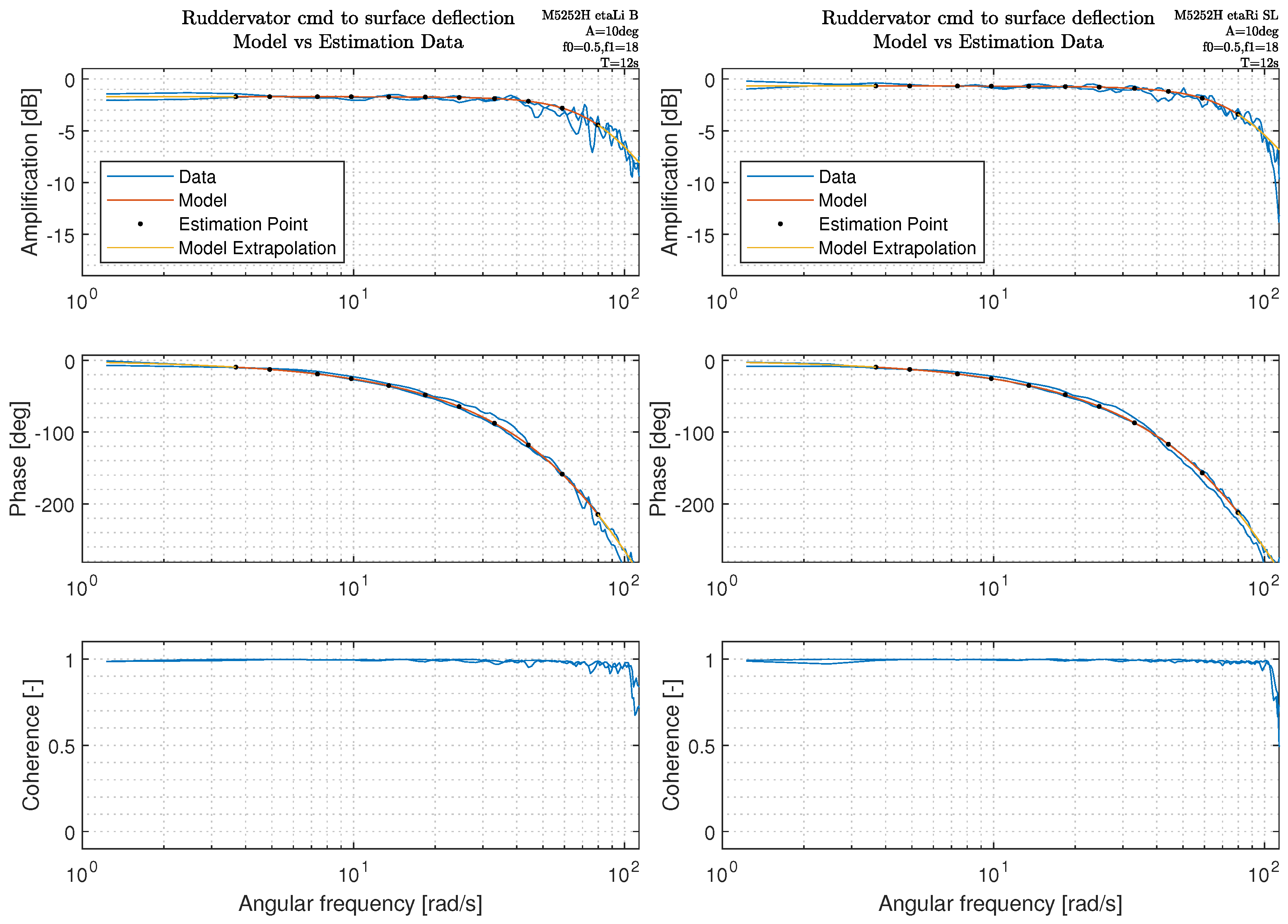
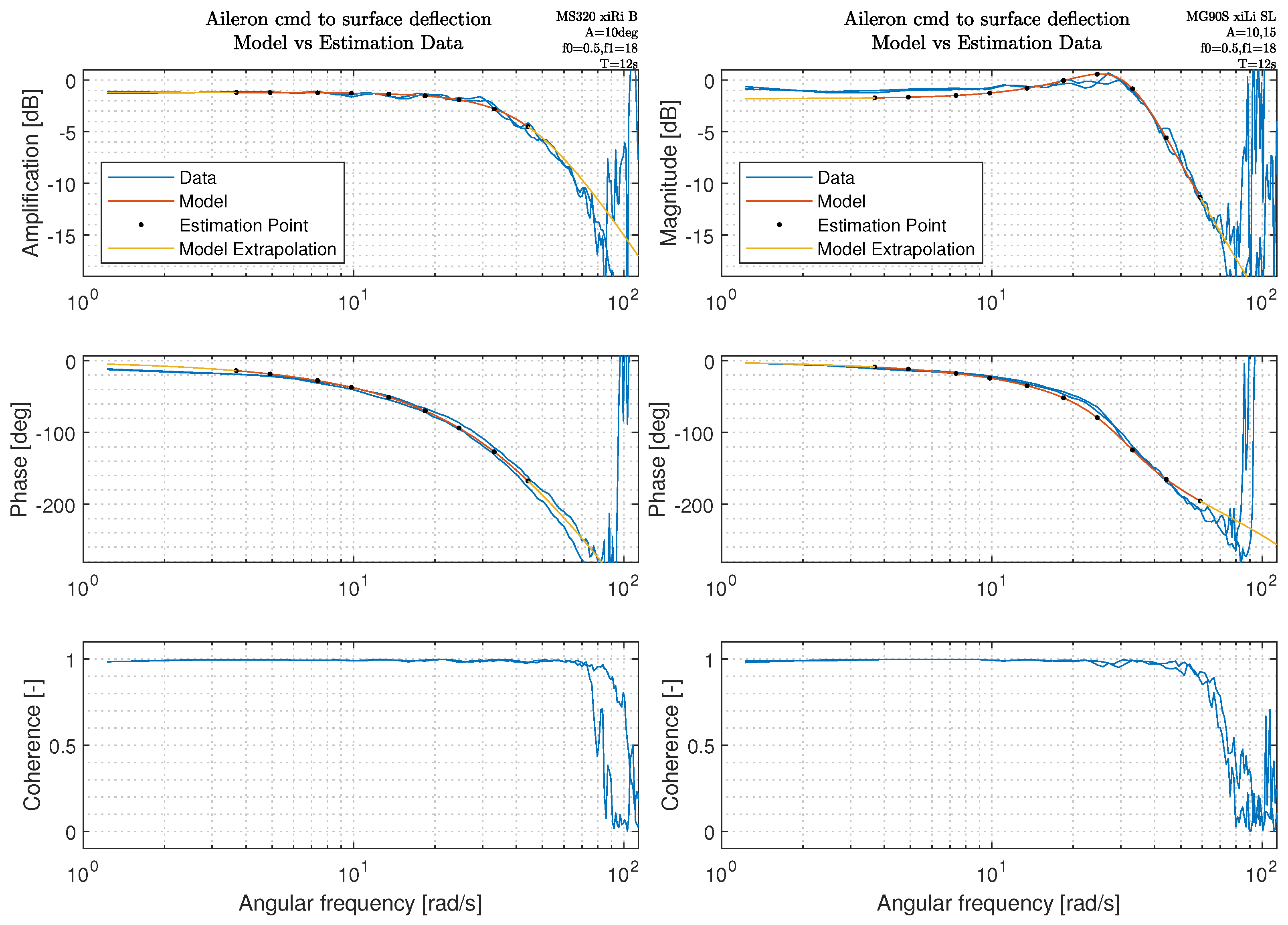
3.4. Model Estimation
3.5. Actuator Discussion
- A second-order system with time delay can be used to reasonably represent the dynamics for most of the actuators both on ground and in flight, at least up to approximately the bandwidth frequency. The faster actuators M5251H and M5252H have the best model fit. It may be considered to increase the model order for the slower MG90S and MS320 to obtain a better fit.
- The reduction in bandwidth from ground to in flight at the given conditions is at maximum ∼10%.
- There can be significant in-flight bias (DC offset) between actuator/surface command and surface position.
- There is noticeable reduction in gain () between ground and in-air tests.
- The M5252H actuator, which has both high torque and high speed indicated in the datasheet, has significantly higher bandwidth than the other actuators.
- The frequency response of the actuator in flight is reproducible with good accuracy.
- High coherence values extend to higher frequencies for M5252H and M5251H than for the MG90S.
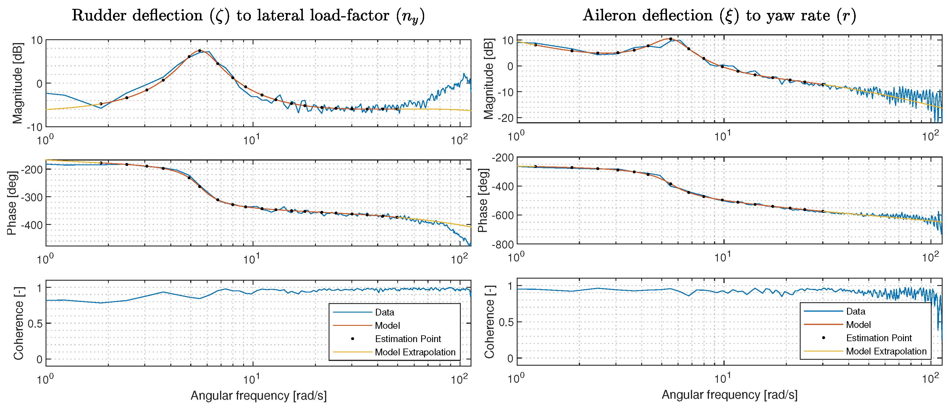
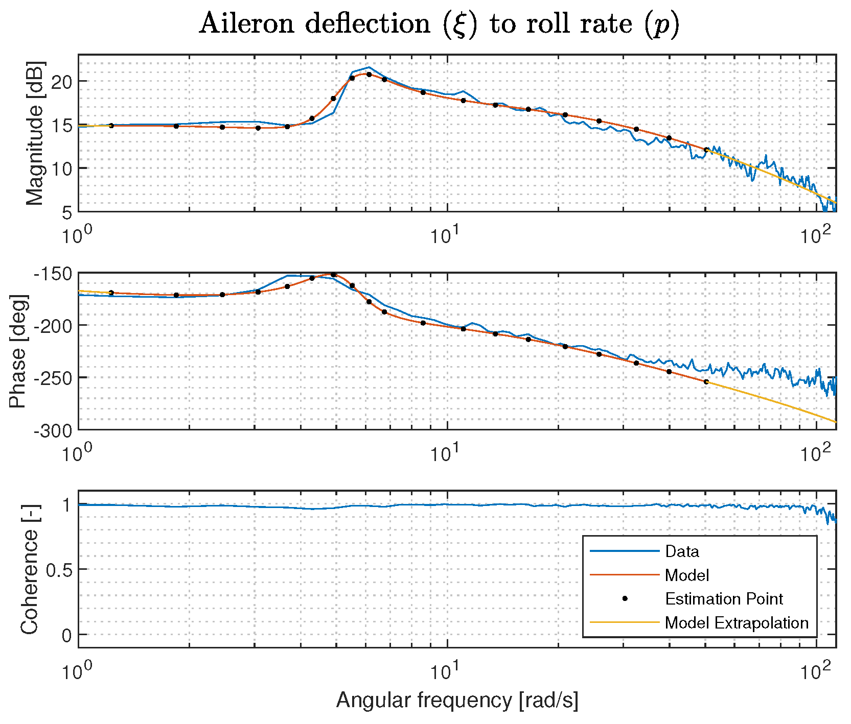
4. Identification of Flight Dynamic Model
4.1. Model Structure: Linear-Directional Lateral Dynamics
4.2. Experiment Design
4.3. Estimation Data
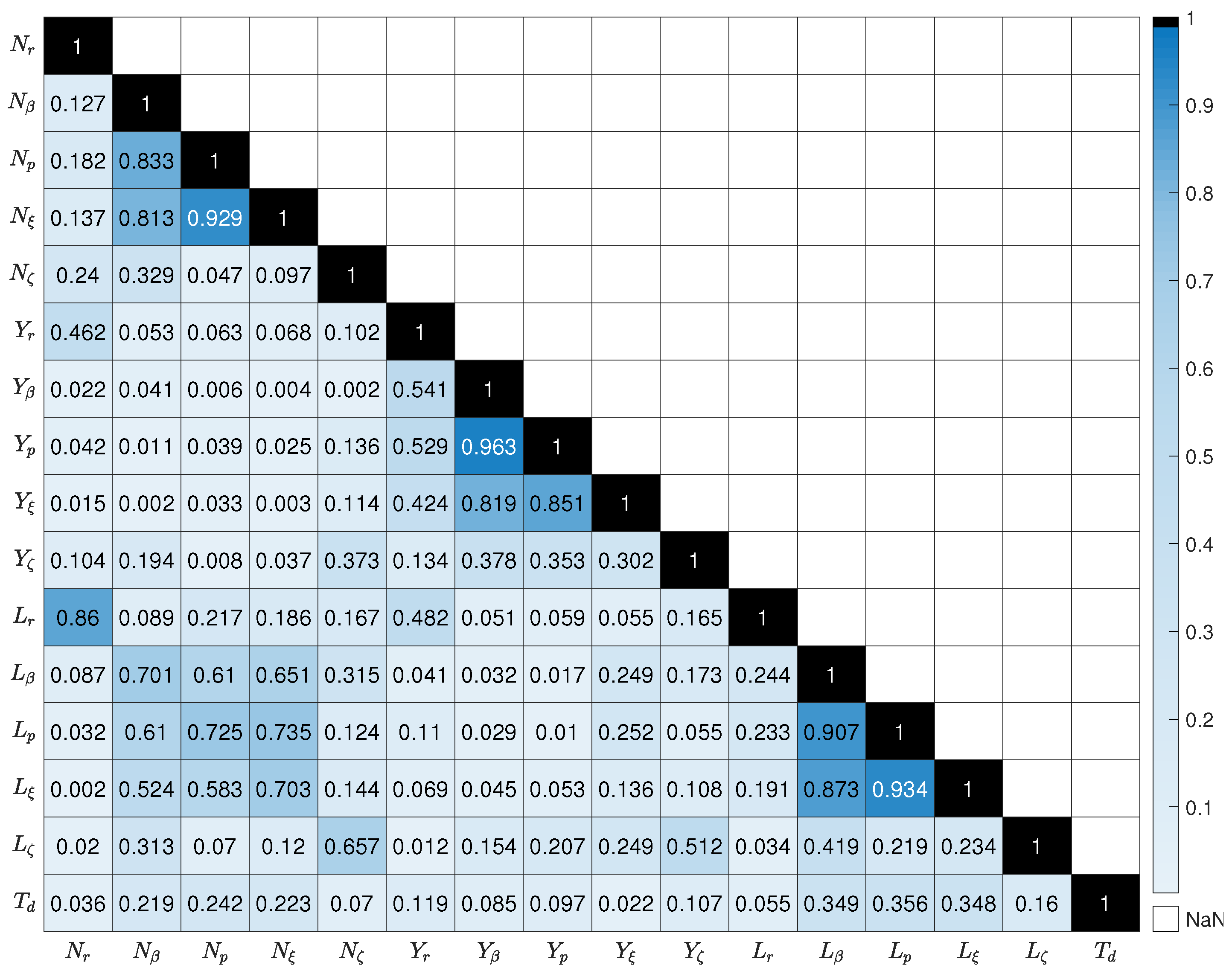
4.4. Parameter Estimation
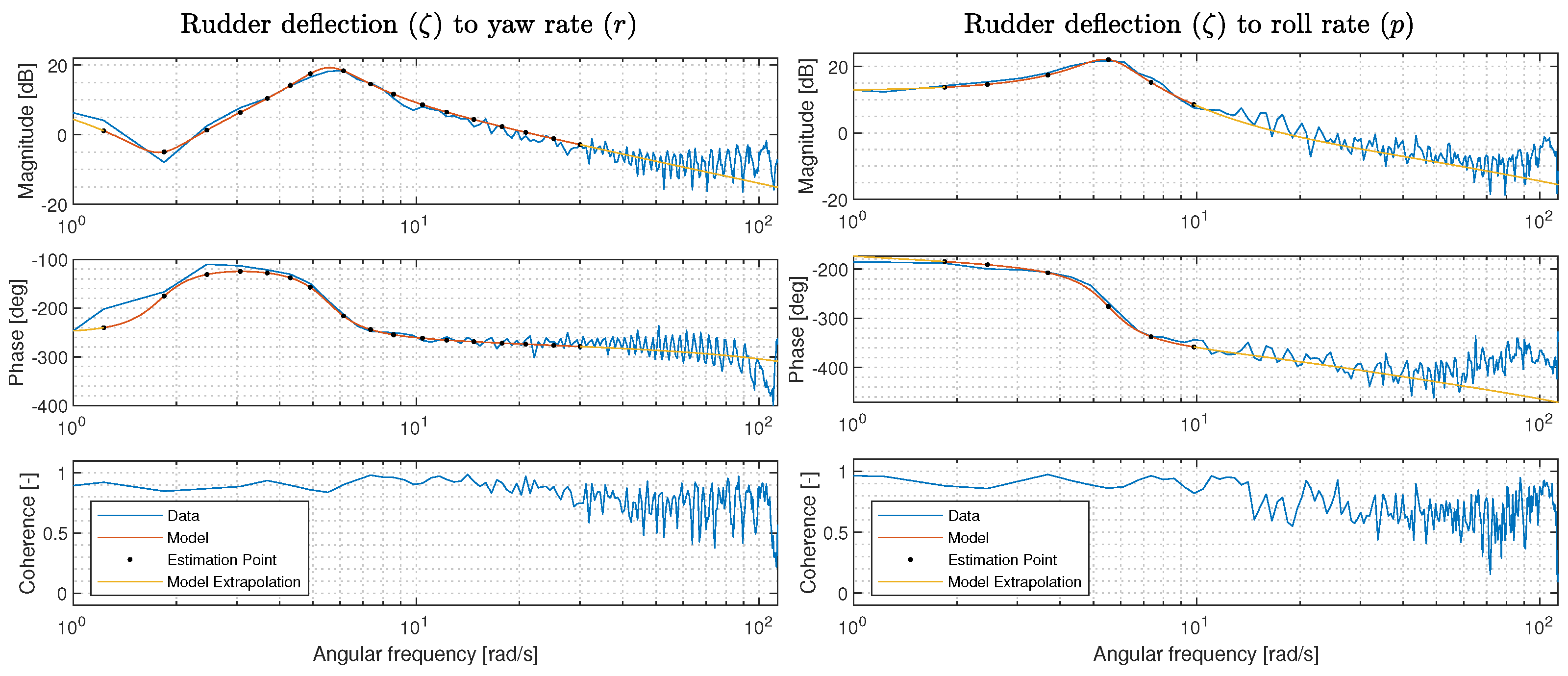
4.5. Estimation Results
5. Control Design and Evaluation
- Avoids hidden coupling terms when scheduling the controller gains;
- Bump less transfer between different gain groups;
- Enhanced integrator wind-up prevention;
- Robust performance with respect to variations in model parameters;
- Enhanced disturbance rejection;
- Less sensitive to unknown time delays at the input.
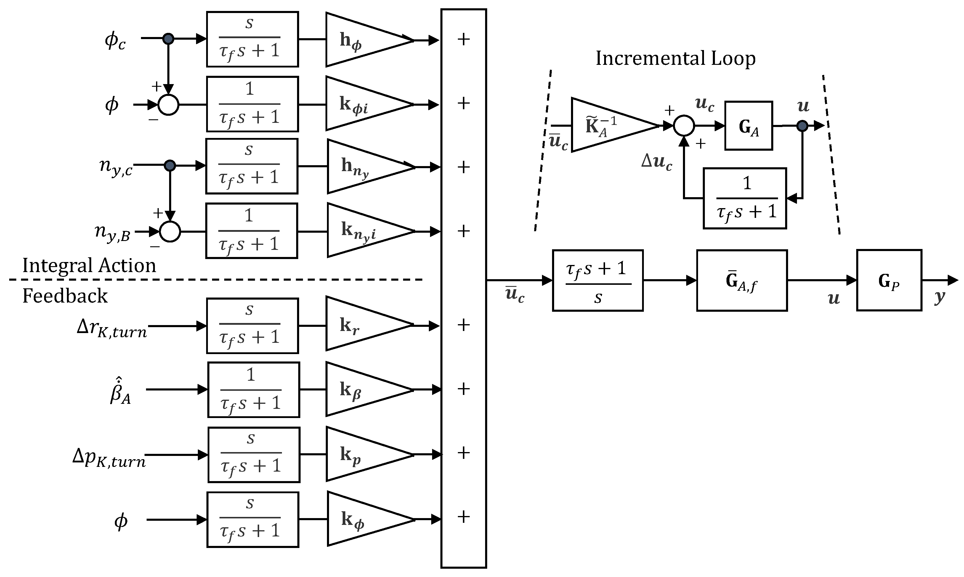
5.1. Control Law Structure
5.2. Flow Angle Derivatives for State Feedback
5.3. Turn Coordination
5.4. Gain Design
- Integral behavior by assigning closed-loop integrator poles as given by Table 5.
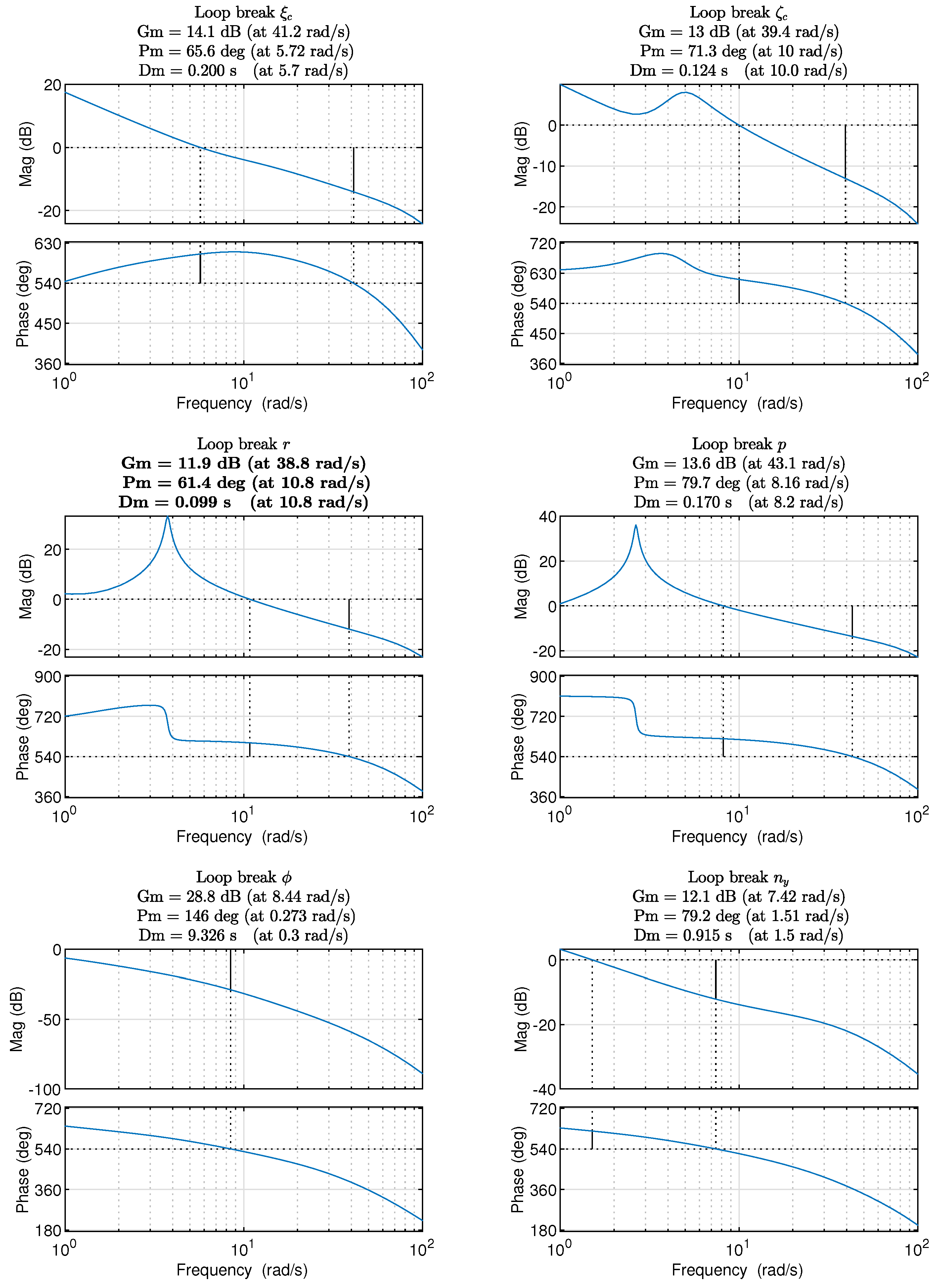
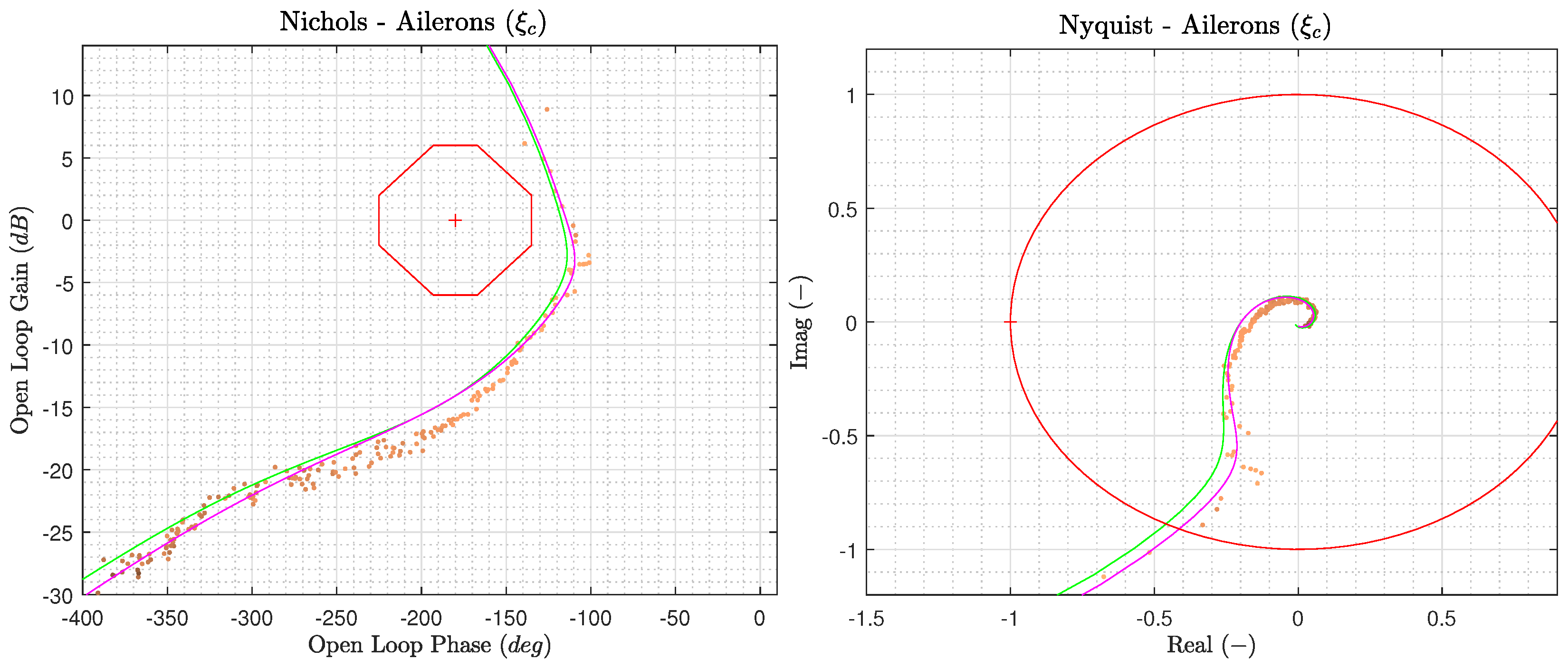
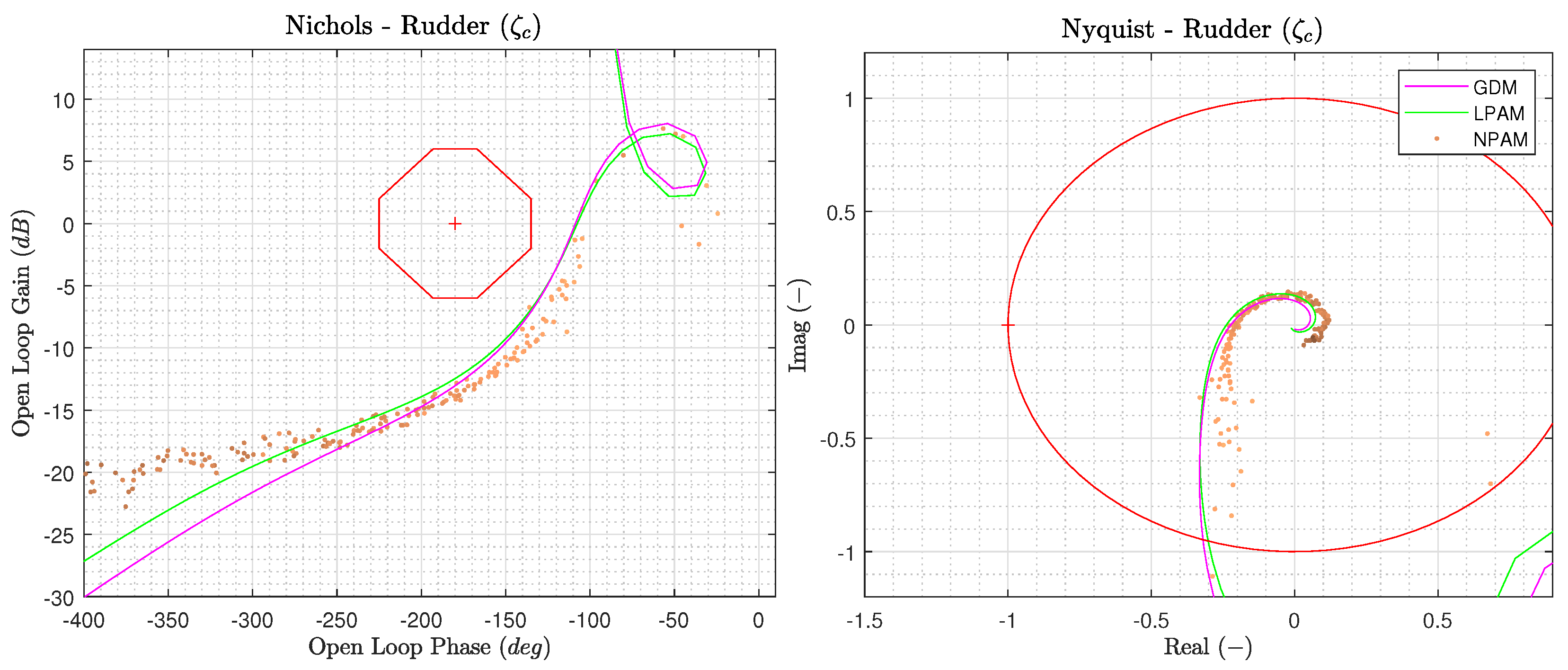
- Gain margin (>6 dB) and phase margin (>). Additionally, it is sought to have the time delay margin above four samples (>0.04 s). The final design margins are shown in Figure 17.
- Limit the gain and phase crossover frequencies to below 45 rad/s in order to provide sufficient margin against model uncertainties at higher frequencies.
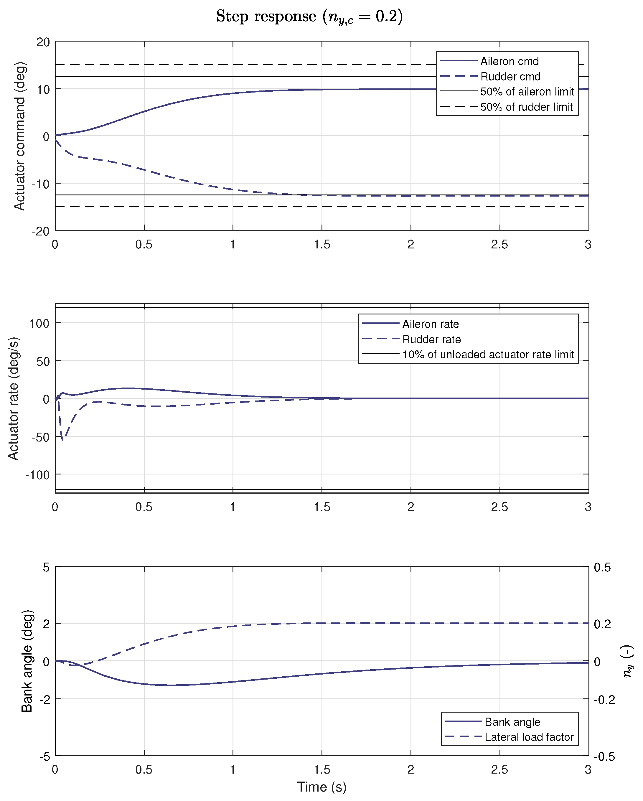
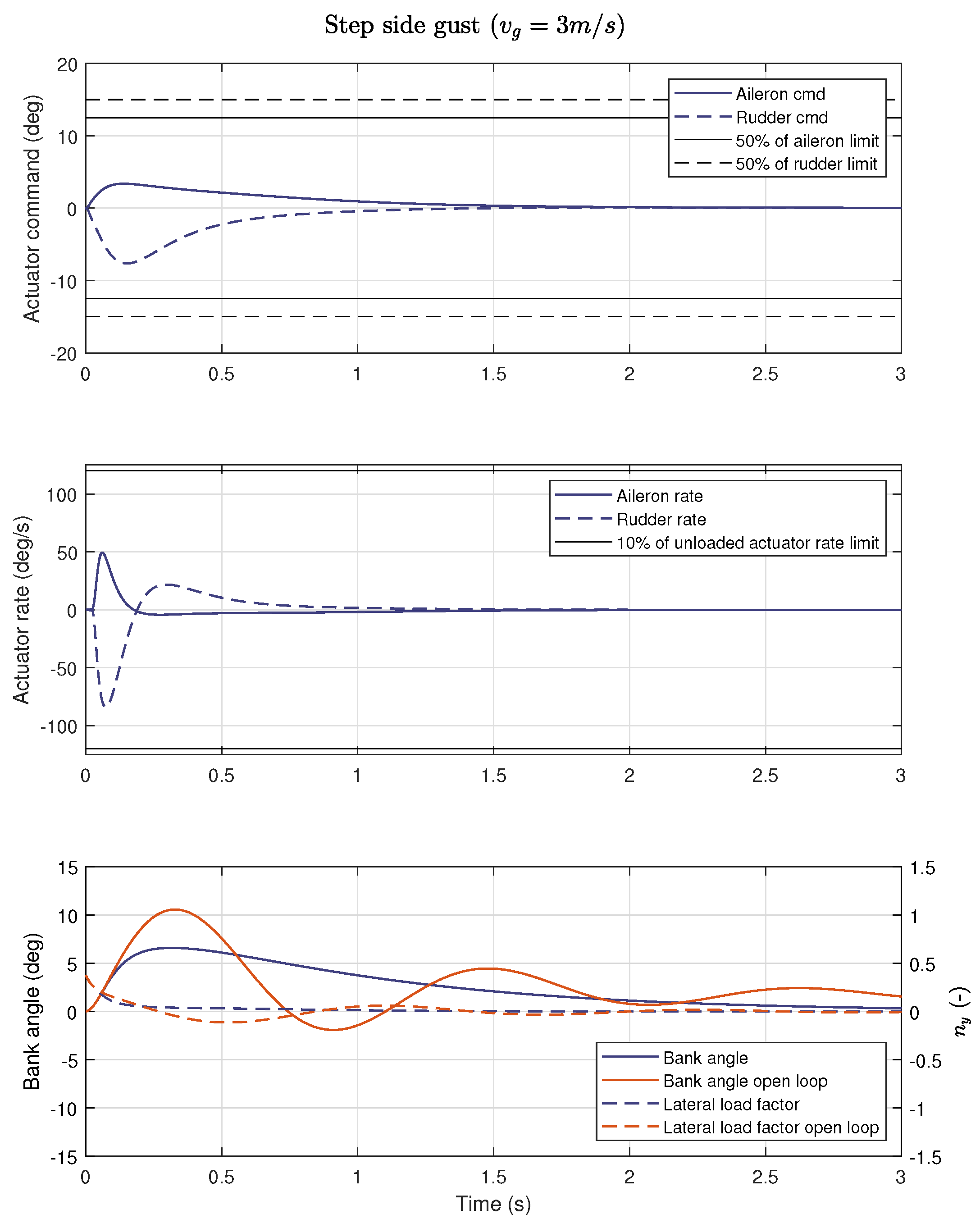
- Limitations on maximum actuator rate and position in relation to step commands and gusts as depicted in Figure 18 and Figure 19. The following limits are empirically found to work, but should be increased and verified via further flight test. For a step gust of m/s or command , the actuator rate is sought to be less than of the unloaded maximum, and the actuator position less than of the maximum.
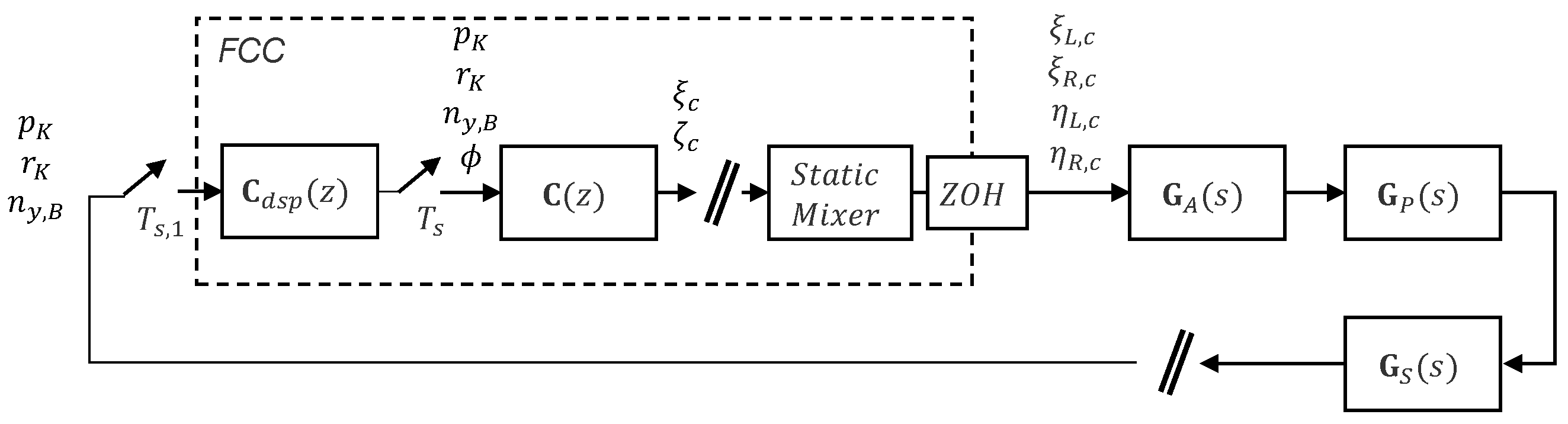
5.5. Implementation
5.6. Assessment
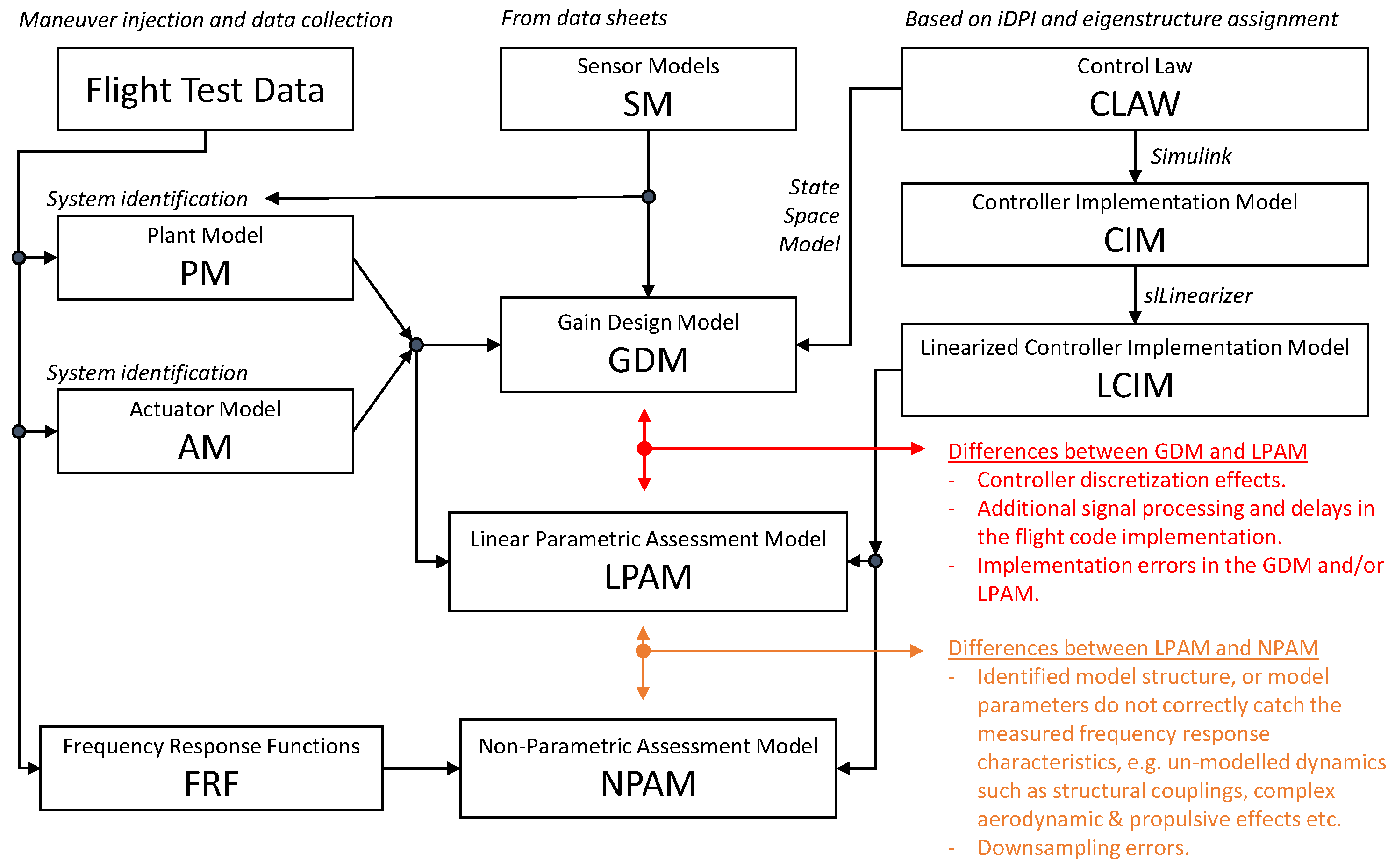
- Gain design model (GDM):Linear continuous time model, possibly with simplifications used to calculate the controller gains.
- Linear parametric assessment model (LPAM):Discrete time linearization of the controller implementation model connected with the zoh transform of the identified linear continuous time parametric models of the actuators, plant and sensors. The zero order hold transform is used because the controller outputs commands that are held between each time update of the controller, i.e., zero order hold of the commands; using the zoh transform for assessment correctly represents the dynamics of the sampled closed-loop continuous time system.
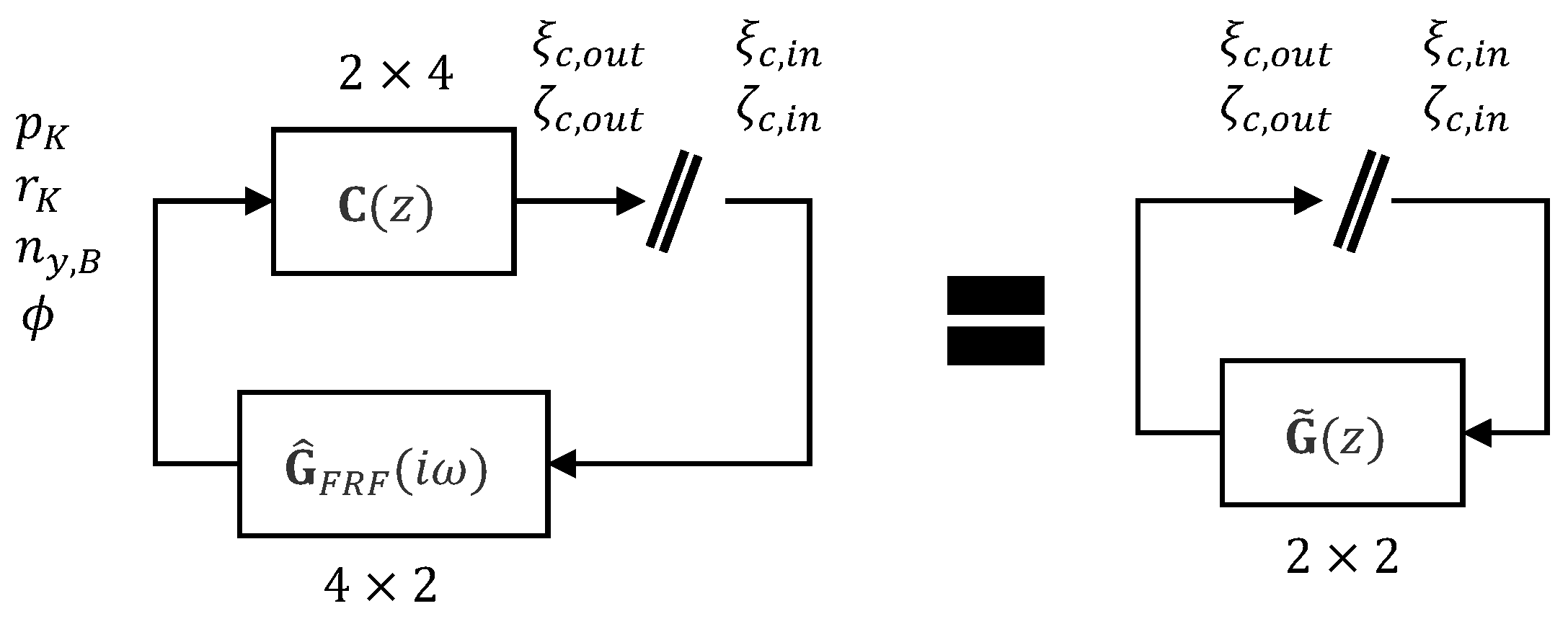
- Non-parametric assessment model (NPAM):Discrete time linearization of the controller implementation model connected with the non-parametric frequency response estimates from flight test.
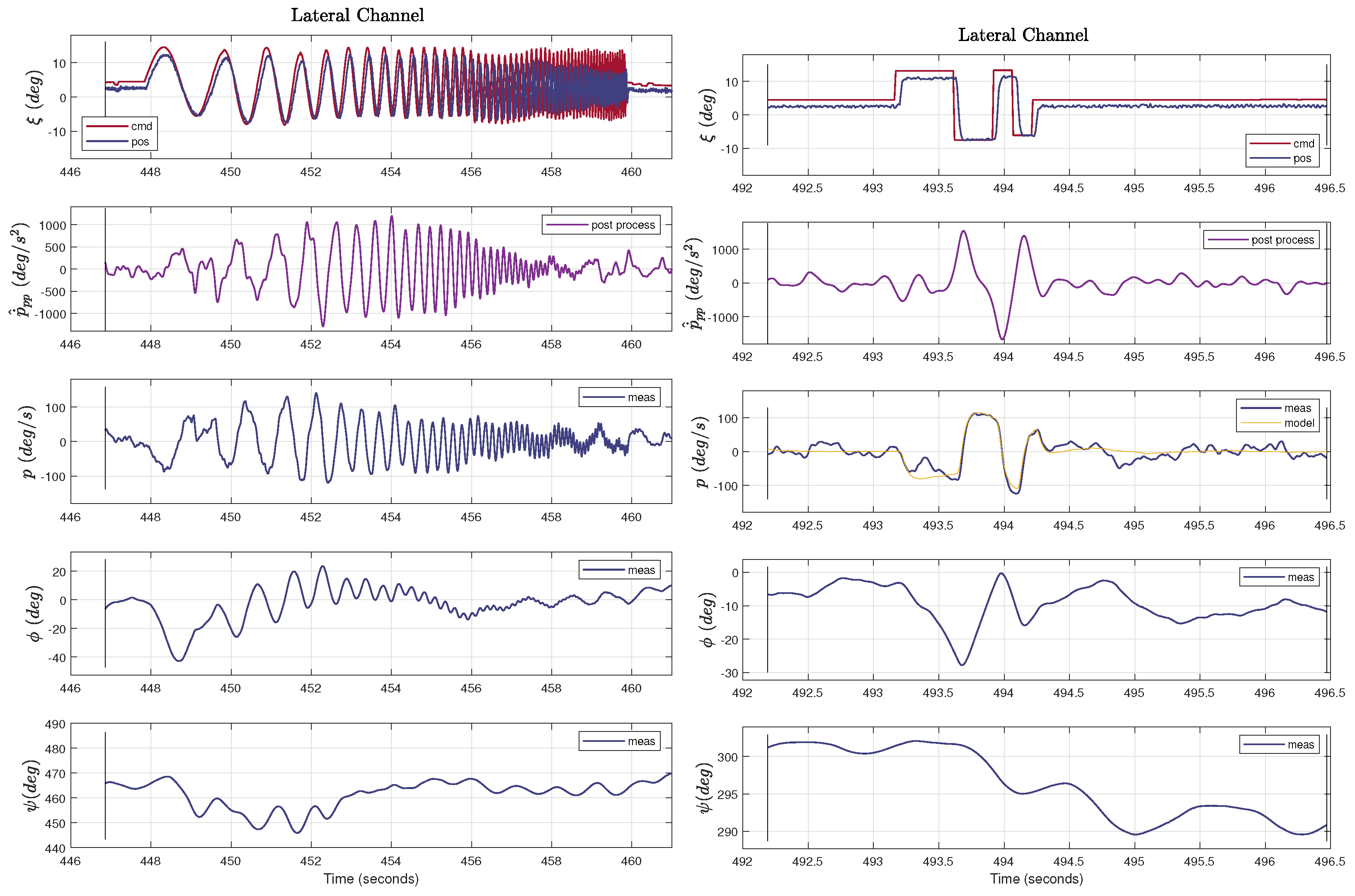
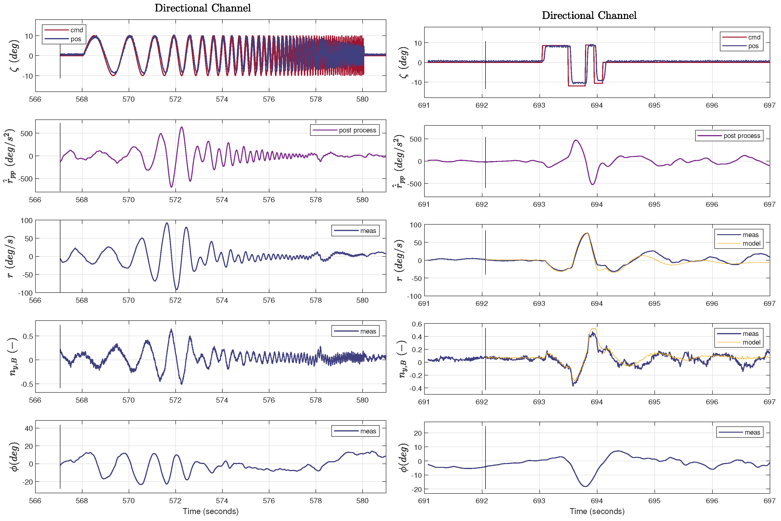
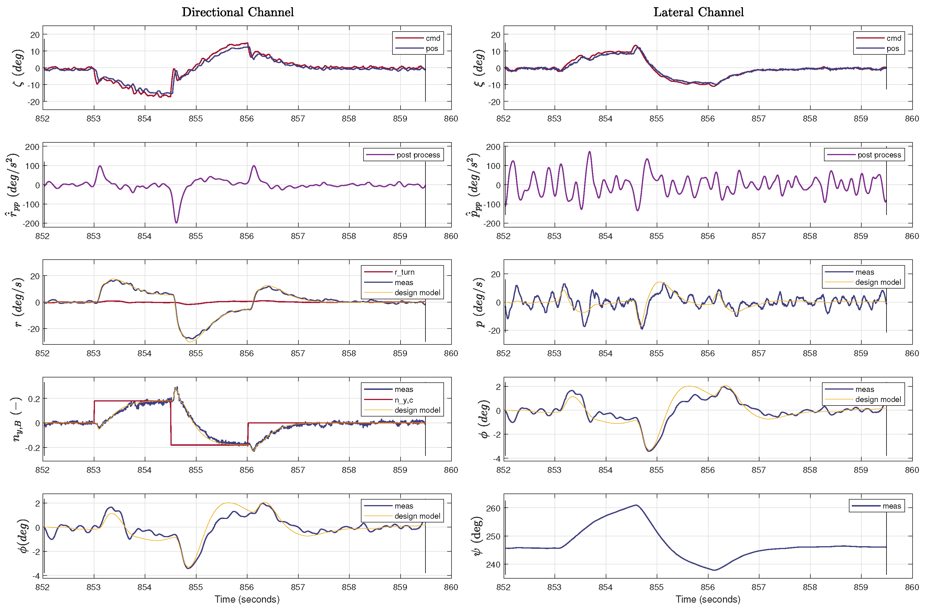
5.7. Lateral Flight Test Results
6. Conclusions
Author Contributions
Funding

Data Availability Statement
Acknowledgments
Conflicts of Interest
Appendix A
Appendix B
Appendix C
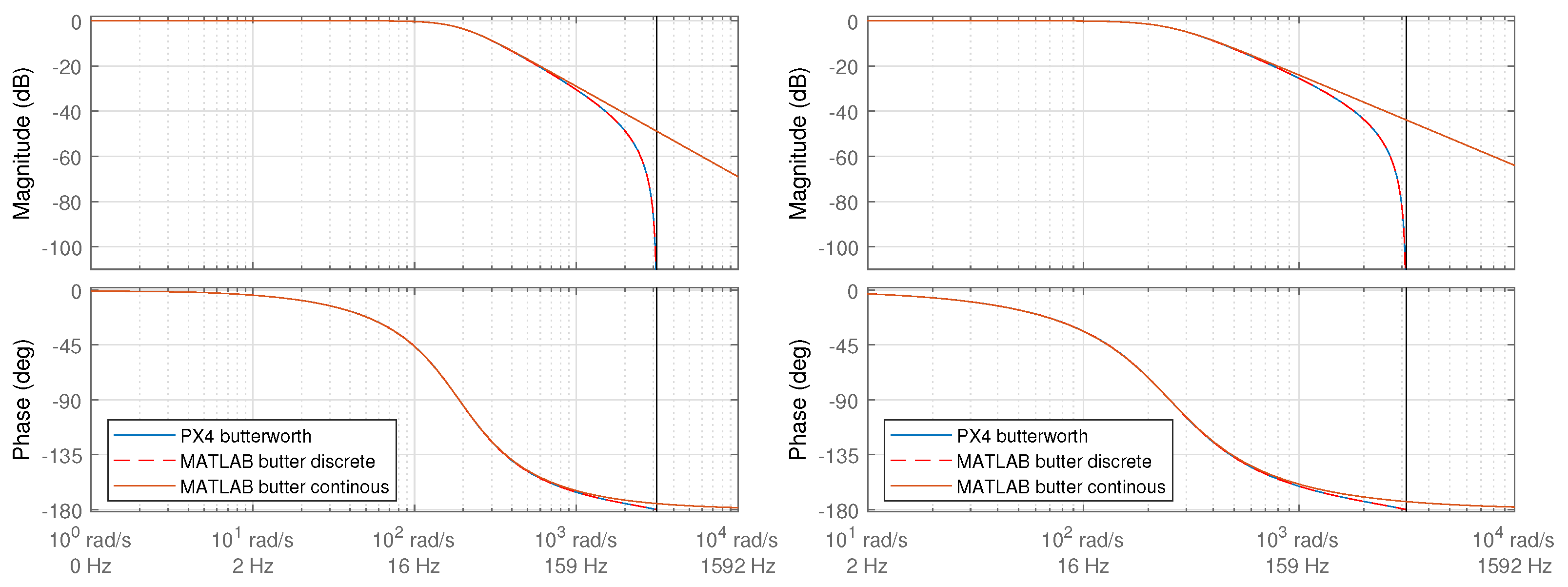
Appendix C.1. PX4 Sensor Downsampling Filter

Appendix D
Appendix D.1. Calculation of Non-Parametric Loop Break
References
- Steffensen, R.; Steinert, A.; Holzapfel, F. Incremental control as an enhanced and robust implementation of gain scheduled controllers avoiding hidden coupling terms. Aerosp. Sci. Technol. 2023, 141, 108500. [Google Scholar] [CrossRef]
- Bacon, B.; Ostroff, A. Reconfigurable flight control using nonlinear dynamic inversion with a special accelerometer implementation. In Proceedings of the AIAA Guidance, Navigation, and Control Conference and Exhibit, Denver, CO, USA, 14–17 August 2000; p. 4565. [Google Scholar]
- Sieberling, S.; Chu, Q.; Mulder, J. Robust flight control using incremental nonlinear dynamic inversion and angular acceleration prediction. J. Guid. Control Dyn. 2010, 33, 1732–1742. [Google Scholar] [CrossRef]
- Morelli, E.A.; Klein, V. Aircraft System Identification: Theory and Practice; Sunflyte Enterprises: Williamsburg, VA, USA, 2016; Volume 2. [Google Scholar]
- Tischler, M.B.; Remple, R.K. Aircraft and Rotorcraft System Identification; American Institute of Aeronautics and Astronautics: Reston, VA, USA, 2012. [Google Scholar]
- Jategaonkar, R.V. Flight Vehicle System Identification: A Time Domain Methodology; American Institute of Aeronautics and Astronautics: Reston, VA, USA, 2006. [Google Scholar]
- Cooper, J.K.; DeVore, M.; Reed, A.; Morelli, E.A. Deterministic and Probabilistic Approaches to Model and Update Dynamic Systems. J. Aircr. 2023, 60, 1461–1479. [Google Scholar] [CrossRef]
- Morelli, E.A.; Grauer, J.A. Advances in Aircraft System Identification at NASA Langley Research Center. J. Aircr. 2023, 60, 1354–1370. [Google Scholar] [CrossRef]
- Leshikar, C.; Valasek, J.; McQuinn, C.K. System Identification of Unmanned Air Systems at Texas A&M University. J. Aircr. 2023, 60, 1437–1460. [Google Scholar]
- Hosseini, B.; Steinert, A.; Hofmann, R.; Fang, X.; Steffensen, R.; Holzapfel, F.; Göttlicher, C. Advancements in the Theory and Practice of Flight Vehicle System Identification. J. Aircr. 2023, 60, 1419–1436. [Google Scholar] [CrossRef]
- Grauer, J.A.; Boucher, M.J. Aircraft system identification from multisine inputs and frequency responses. J. Guid. Control Dyn. 2020, 43, 2391–2398. [Google Scholar] [CrossRef]
- Lampton, A.K.; Klyde, D.H.; Schulze, P.C. Overview of System Identification Tool Advancements at Systems Technology, Incorporated. J. Aircr. 2023, 60, 1522–1537. [Google Scholar] [CrossRef]
- Grauer, J.A. Frequency Response Estimation for Multiple Aircraft Control Loops Using Orthogonal Phase-Optimized Multisine Inputs. Processes 2022, 10, 619. [Google Scholar] [CrossRef]
- Grauer, J.A.; Morelli, E.A. Introduction to the Advances in Aircraft System Identification from Flight Test Data Virtual Collection. J. Aircr. 2023, 60, 1329–1330. [Google Scholar] [CrossRef]
- De Visser, C.C.; Pool, D.M. Stalls and Splines: Current Trends in Flight Testing and Aerodynamic Model Identification. J. Aircr. 2023, 60, 1480–1502. [Google Scholar] [CrossRef]
- Caetano, J.V.; De Visser, C.; De Croon, G.; Remes, B.; De Wagter, C.; Verboom, J.; Mulder, M. Linear aerodynamic model identification of a flapping wing mav based on flight test data. Int. J. Micro Air Veh. 2013, 5, 273–286. [Google Scholar] [CrossRef]
- Subedi, S.; Hosseini, B.; Diepolder, J.; Holzapfel, F. Online parameter identification and optimal input design using perturbed nonlinear programming. J. Phys. Conf. Ser. 2023, 2514, 012020. [Google Scholar] [CrossRef]
- Hofmann, R.; Hosseini, S.; Fang, X.; Holzapfel, F. Flight Path Reconstruction for a Coaxial Helicopter Equipped with Rotational Accelerometers. In Proceedings of the AIAA AVIATION 2023 Forum, San Diego, CA, US, 12–16 June 2023; p. 3292. [Google Scholar]
- Larsson, R.; Sobron, A.; Lundström, D.; Enqvist, M. A method for improved flight testing of remotely piloted aircraft using multisine inputs. Aerospace 2020, 7, 135. [Google Scholar] [CrossRef]
- Simmons, B.M.; Gresham, J.L.; Woolsey, C.A. Flight-Test System Identification Techniques and Applications for Small, Low-Cost, Fixed-Wing Aircraft. J. Aircr. 2023, 60, 1503–1521. [Google Scholar] [CrossRef]
- Hofmann, R.; Hosseini, S.; Holzapfel, F. Flight-Test Plan Design and Evaluation in a Closed-Loop Framework for a General Aviation Aircraft. In Proceedings of the AIAA SCITECH 2022 Forum, San Diego, CA, USA, 3–7 January 2022; p. 2170. [Google Scholar]
- Bachfischer, M.; Hosseini, S.; Sax, F.; Rhein, J.; Holzapfel, F.; Maier, L.; Barth, A. Linear Model Identification for a Coaxial Rotorcraft in Hover. In Proceedings of the AIAA SCITECH 2024 Forum, Orlando, FL, USA, 8–12 January 2024; p. 1719. [Google Scholar]
- Hosseini, B.; Sax, F.; Rhein, J.; Holzapfel, F.; Maier, L.; Barth, A.; Hajek, M.; Grebing, B. Global Model Identification for a Coaxial Helicopter. In Proceedings of the Vertical Flight Society 78th Annual Forum, Fort Worth, TX, USA, 10–12 May 2022. [Google Scholar]
- Hosseini, S.; Mbikayi, Z.; Bachfischer, M.; Holzapfel, F.; Rauleder, J. Simulation, Flight Dynamics, and Control Design for a Coaxial Rotorcraft. In Proceedings of the AIAA Scitech 2024 Forum, Orlando, FL, USA, 8–12 January 2024; p. 1717. [Google Scholar]
- Hofmann, R.; Hosseini, S.; Fang, X.; Rhein, J.; Sax, F.; Holzapfel, F.; Maier, L.; Barth, A. Center of Gravity Estimation Using Multiple Accelerometers. In Proceedings of the AIAA Scitech 2024 Forum, Orlando, FL, USA, 8–12 January 2024; p. 1721. [Google Scholar]
- Lichota, P.; Szulczyk, J.; Tischler, M.B.; Berger, T. Frequency responses identification from multi-axis maneuver with simultaneous multisine inputs. J. Guid. Control Dyn. 2019, 42, 2550–2556. [Google Scholar] [CrossRef]
- Berger, T.; Tobias, E.L.; Tischler, M.B.; Juhasz, O. Advances and Modern Applications of Frequency-Domain Aircraft and Rotorcraft System Identification. J. Aircr. 2023, 60, 1331–1353. [Google Scholar] [CrossRef]
- Niermeyer, P.; Raffler, T.; Holzapfel, F. Open-loop quadrotor flight dynamics identification in frequency domain via closed-loop flight testing. In Proceedings of the AIAA Guidance, Navigation, and Control Conference, Kissimmee, FL, USA, 5–9 January 2015; p. 1539. [Google Scholar]
- Steinert, A.; Steffensen, R.; Gierszewski, D.; Speckmaier, M.; Holzapfel, F.; Schmoldt, R.; Demmler, F.; Schell, U.; Ornigg, M.; Koop, M. Experimental Results of Flight Test Based Gain Tuning. In Proceedings of the AIAA SCITECH 2022 Forum, San Diego, CA, USA, 3–7 January 2022; p. 2296. [Google Scholar]
- Li, H.; Myschik, S.; Holzapfel, F. Null-Space-Excitation-Based Adaptive Control for an Overactuated Hexacopter Model. J. Guid. Control Dyn. 2023, 46, 483–498. [Google Scholar] [CrossRef]
- Hafner, S.F.; Hosseini, S.; Holzapfel, F. Excitation Monitoring for Online Parameter Estimation. In Proceedings of the AIAA SCITECH 2023 Forum, Gaylord National Harbor, MD, USA, 23–27 January 2023; p. 0039. [Google Scholar]
- Akkinapalli, V.S.; Falconí, G.P.; Holzapfel, F. Fault tolerant incremental attitude control using online parameter estimation for a multicopter system. In Proceedings of the 2017 25th Mediterranean Conference on Control and Automation (MED), Valletta, Malta, 3–6 July 2017; pp. 454–460. [Google Scholar]
- Ignatyev, D.I.; Shin, H.S.; Tsourdos, A. Sparse online Gaussian process adaptation for incremental backstepping flight control. Aerosp. Sci. Technol. 2023, 136, 108157. [Google Scholar] [CrossRef]
- Teubl, D.; Bitenc, T.; Hornung, M. Design and Development of an Actuator Control and Monitoring Unit for Small and Medium Size Research Uavs; Deutsche Gesellschaft für Luft-und Raumfahrt-Lilienthal-Oberth eV: Bonn, Germany, 2021. [Google Scholar]
- Teubl, D.; Oberschwendtner, S.; Hornung, M. Measurement Results of the ACMU System in Various Research UAVs. In Proceedings of the AIAA SCITECH 2023 Forum, Gaylord National Harbor, MD, USA, 23–27 January 2023; p. 0481. [Google Scholar]
- Oberschwendtner, S.; Teubl, D.; Hornung, M. Static Test Procedure for Electromechanical Actuators for UAV Applications. In Proceedings of the AIAA AVIATION 2022 Forum, Chicago, IL, USA, 27 June–1 July 2022; p. 3558. [Google Scholar]
- Mancinelli, A.; van der Horst, E.; Remes, B.; Smeur, E. Autopilot framework with INDI RPM control, real-time actuator feedback, and stability control on companion computer through MATLAB generated functions. In Proceedings of the 14th Annual International Micro Air Vehicle Conference and Competition, Aachen, Germany, 11–15 September 2023; pp. 109–116. [Google Scholar]
- Mancinelli, A.; Remes, B.D.; De Croon, G.C.; Smeur, E.J. Real-Time Nonlinear Control Allocation Framework for Vehicles with Highly Nonlinear Effectors Subject to Saturation. J. Intell. Robot. Syst. 2023, 108, 67. [Google Scholar] [CrossRef]
- Osterhuber, R.; Hanel, M.; Hammon, R. Realization of the Eurofighter 2000 primary lateral/directional flight control laws with differential PI-algorithm. In Proceedings of the AIAA Guidance, Navigation, and Control Conference and Exhibit, Providence, RI, USA, 16–19 August 2004; p. 4751. [Google Scholar]
- Wang, X.; Kong, W.; Zhang, D.; Shen, L. Active disturbance rejection controller for small fixed-wing UAVs with model uncertainty. In Proceedings of the 2015 IEEE International Conference on Information and Automation, Lijiang, China, 8–10 August 2015; pp. 2299–2304. [Google Scholar]
- Barth, J.M.; Condomines, J.P.; Moschetta, J.M.; Join, C.; Fliess, M. Model-free control approach for fixed-wing UAVs with uncertain parameters analysis. In Proceedings of the 2018 23rd International Conference on Methods & Models in Automation & Robotics (MMAR), Miedzyzdroje, Poland, 27–30 August 2018; pp. 527–532. [Google Scholar]
- Palframan, M.C.; Fry, J.M.; Farhood, M. Robustness analysis of flight controllers for fixed-wing unmanned aircraft systems using integral quadratic constraints. IEEE Trans. Control Syst. Technol. 2017, 27, 86–102. [Google Scholar] [CrossRef]
- Oudin, S. Low Speed Protections for a Commercial Airliner: A Practical Approach. In Proceedings of the AIAA Guidance, Navigation, and Control Conference, Grapevine, TX, USA, 9–13 January 2017; p. 1023. [Google Scholar]
- Liu, C.; Chen, W.H. Disturbance rejection flight control for small fixed-wing unmanned aerial vehicles. J. Guid. Control Dyn. 2016, 39, 2810–2819. [Google Scholar] [CrossRef]
- Baldi, S.; Roy, S.; Yang, K.; Liu, D. An underactuated control system design for adaptive autopilot of fixed-wing drones. IEEE/ASME Trans. Mechatronics 2022, 27, 4045–4056. [Google Scholar] [CrossRef]
- Reinhardt, D.P. On Nonlinear and Optimization-based Control of Fixed-Wing Unmanned Aerial Vehicles. Ph.D. Thesis, NTNU, Trondheim, Norway, 2022. [Google Scholar]
- Lavretsky, E. Design, analysis, and flight evaluation of a primary control system with observer-based loop transfer recovery and direct adaptive augmentation for the calspan variable stability simulator learjet-25b aircraft. In Proceedings of the AIAA Scitech 2019 Forum, San Diego, CA, USA, 7–11 January 2019; p. 1081. [Google Scholar]
- Weiser, C.; Ossmann, D.; Kuchar, R.O.; Müller, R.; Milz, D.M.; Looye, G. Flight testing a linear parameter varying control law on a passenger aircraft. In Proceedings of the AIAA Scitech 2020 Forum, Orlando, FL, USA, 6–10 January 2020; p. 1618. [Google Scholar]
- Lombaerts, T.; Chu, Q.; Mulder, J.; Joosten, D. Modular flight control reconfiguration design and simulation. Control Eng. Pract. 2011, 19, 540–554. [Google Scholar] [CrossRef]
- Lombaerts, T.; Mulder, J.; Voorsluijs, G.; Decuypere, R. Design of a robust flight control system for a mini-UAV. In Proceedings of the AIAA Guidance, Navigation, and Control Conference and Exhibit, San Francisco, CA, USA, 15–18 August 2005; p. 6408. [Google Scholar]
- Weiser, C.; Schulz, S.; Voss, A.; Ossmann, D. Attitude Control for High Altitude Long Endurance Aircraft Considering Structural Load Limits. In Proceedings of the AIAA SciTech 2023 Forum, Gaylord National Harbor, MD, USA, 23–27 January 2023; p. 0106. [Google Scholar]
- Kim, Y.; Kim, S.; Suk, J. Incremental Nonlinear Dynamic Inversion-based Fault-Tolerant Guidance for UAV. In Proceedings of the AIAA SCITECH 2024 Forum, Orlando, FL, USA, 8–12 January 2024; p. 2564. [Google Scholar]
- Stougie, J.; Pollack, T.; Van Kampen, E.J. Incremental Nonlinear Dynamic Inversion control with Flight Envelope Protection for the Flying-V. In Proceedings of the AIAA SCITECH 2024 Forum, Orlando, FL, USA, 8–12 January 2024; p. 2565. [Google Scholar]
- Pfeifle, O.; Fichter, W. Minimum power control allocation for incremental control of over-actuated transition aircraft. J. Guid. Control Dyn. 2023, 46, 286–300. [Google Scholar] [CrossRef]
- Konatala, R.B.; Van Kampen, E.J.; Looye, G.; Milz, D.; Weiser, C. Flight Testing Reinforcement Learning based Online Adaptive Flight Control Laws on CS-25 Class Aircraft. In Proceedings of the AIAA SCITECH 2024 Forum, Orlando, FL, USA, 8–12 January 2024; p. 2402. [Google Scholar]
- Smeur, E.J.; Bronz, M.; de Croon, G.C. Incremental control and guidance of hybrid aircraft applied to a tailsitter unmanned air vehicle. J. Guid. Control Dyn. 2020, 43, 274–287. [Google Scholar] [CrossRef]
- Athayde, A.; Moutinho, A.; Azinheira, J.R. Experimental Nonlinear and Incremental Control Stabilization of a Tail-Sitter UAV with Hardware-in-the-Loop Validation. Preprint 2024. [Google Scholar] [CrossRef]
- Beyer, Y.; Steen, M.; Hecker, P. Incremental passive fault-tolerant control for quadrotors subjected to complete rotor failures. J. Guid. Control Dyn. 2023, 46, 2033–2042. [Google Scholar] [CrossRef]
- Pollack, T.; Van Kampen, E.J. Robust Stability and Performance Analysis of Incremental Dynamic-Inversion-Based Flight Control Laws. J. Guid. Control Dyn. 2023, 46, 1785–1798. [Google Scholar] [CrossRef]
- Azinheira, J.R.; Moutinho, A.; Carvalho, J. Lateral control of airship with uncertain dynamics using incremental nonlinear dynamics inversion. IFAC-Pap. 2015, 48, 69–74. [Google Scholar] [CrossRef]
- Wang, X.; Sun, S. Incremental fault-tolerant control for a hybrid quad-plane UAV subjected to a complete rotor loss. Aerosp. Sci. Technol. 2022, 125, 107105. [Google Scholar] [CrossRef]
- Cordeiro, R.A.; Azinheira, J.R.; Moutinho, A. Robustness of Incremental Backstepping Flight Controllers: The Boeing 747 Case Study. IEEE Trans. Aerosp. Electron. Syst. 2021, 57, 3492–3505. [Google Scholar] [CrossRef]
- Cordeiro, R.A.; Marton, A.S.; Azinheira, J.R.; Carvalho, J.R.; Moutinho, A. Increased robustness to delay in incremental controllers using input scaling gain. IEEE Trans. Aerosp. Electron. Syst. 2021, 58, 1199–1210. [Google Scholar] [CrossRef]
- Jeong, H.; Jeong, J.; Suk, J.; Kim, S. Angular Acceleration Estimation with Off-CG Accelerometers for Incremental Nonlinear Dynamic Inversion Control. In Proceedings of the AIAA SCITECH 2024 Forum, Orlando, FL, USA, 8–12 January 2024; p. 2566. [Google Scholar]
- Smeur, E.J.; Chu, Q.; De Croon, G.C. Adaptive incremental nonlinear dynamic inversion for attitude control of micro air vehicles. J. Guid. Control Dyn. 2016, 39, 450–461. [Google Scholar] [CrossRef]
- De Ponti, T.; Smeur, E.; Remes, B. Incremental Nonlinear Dynamic Inversion controller for a Variable Skew Quad Plane. In Proceedings of the 2023 International Conference on Unmanned Aircraft Systems (ICUAS), Warsaw, Poland, 6–9 June 2023; pp. 241–248. [Google Scholar]
- Smeur, E.J.; de Croon, G.C.; Chu, Q. Cascaded incremental nonlinear dynamic inversion for MAV disturbance rejection. Control Eng. Pract. 2018, 73, 79–90. [Google Scholar] [CrossRef]
- Steffensen, R.; Steinert, A.; Smeur, E.J. Nonlinear Dynamic Inversion with Actuator Dynamics: An Incremental Control Perspective. J. Guid. Control Dyn. 2022, 46, 709–717. [Google Scholar] [CrossRef]
- Steffensen, R.; Steinert, A.; Mbikayi, Z.; Raab, S.; Angelov, J.; Holzapfel, F. Filter and sensor delay synchronization in incremental flight control laws. Aerosp. Syst. 2023, 6, 285–304. [Google Scholar] [CrossRef]
- Steffensen, R.; Steinert, A.; Holzapfel, F. Longitudinal Incremental Reference Model for Fly-By-Wire Control Law using Incremental Non-Linear Dynamic Inversion. In Proceedings of the AIAA Scitech 2022 Forum, San Diego, CA, USA, 3–7 January 2022; p. 1230. [Google Scholar]
- Lu, P.; Van Kampen, E.J.; De Visser, C.; Chu, Q. Aircraft fault-tolerant trajectory control using incremental nonlinear dynamic inversion. Control Eng. Pract. 2016, 57, 126–141. [Google Scholar] [CrossRef]
- Ye, Z.; Chen, Y.; Cai, P.; Lyu, H.; Gong, Z.; Wu, J. Control Design for Soft Transition for Landing Preparation of Light Compound-Wing Unmanned Aerial Vehicles Based on Incremental Nonlinear Dynamic Inversion. Appl. Sci. 2023, 13, 12225. [Google Scholar] [CrossRef]
- Steinleitner, A.; Frenzel, V.; Pfeifle, O.; Denzel, J.; Fichter, W. Automatic take-off and landing of tailwheel aircraft with incremental nonlinear dynamic inversion. In Proceedings of the AIAA Scitech 2022 Forum, San Diego, CA, USA, 3–7 January 2022; p. 1228. [Google Scholar]
- Myschik, S.; Kinast, L.; Huemer, M.; Vicca, D.; Dollinger, D.; Holzapfel, F. Development of a Flight Control System for a Cyclocopter UAV Demonstrator. In Proceedings of the AIAA AVIATION 2022 Forum, San Diego, CA, USA, 3–7 January 2022; p. 3282. [Google Scholar]
- Kumtepe, Y.; Pollack, T.; Van Kampen, E.J. Flight control law design using hybrid incremental nonlinear dynamic inversion. In Proceedings of the AIAA SciTech 2022 Forum, San Diego, CA, USA, 3–7 January 2022; p. 1597. [Google Scholar]
- Raab, S.A.; Zhang, J.; Bhardwaj, P.; Holzapfel, F. Consideration of Control Effector Dynamics and Saturations in an Extended INDI Approach. In Proceedings of the AIAA Aviation 2019 Forum, Dallas, TX, USA, 17–21 June 2019; p. 3267. [Google Scholar]
- Bhardwaj, P.; Akkinapalli, V.S.; Zhang, J.; Saboo, S.; Holzapfel, F. Adaptive augmentation of incremental nonlinear dynamic inversion controller for an extended f-16 model. In Proceedings of the AIAA Scitech 2019 Forum, San Diego, CA, USA, 7–11 January 2019; p. 1923. [Google Scholar]
- Sun, S.; Wang, X.; Chu, Q.; de Visser, C. Incremental nonlinear fault-tolerant control of a quadrotor with complete loss of two opposing rotors. IEEE Trans. Robot. 2020, 37, 116–130. [Google Scholar] [CrossRef]
- Wang, X.; Van Kampen, E.J.; Chu, Q.; Lu, P. Stability analysis for incremental nonlinear dynamic inversion control. J. Guid. Control Dyn. 2019, 42, 1116–1129. [Google Scholar] [CrossRef]
- Schildkamp, R.; Chang, J.; Sodja, J.; De Breuker, R.; Wang, X. Incremental Nonlinear Control for Aeroelastic Wing Load Alleviation and Flutter Suppression. Actuators 2023, 12, 280. [Google Scholar] [CrossRef]
- Surmann, D.; Myschik, S. Gain Design for an INDI-based Flight Control Algorithm for a Conceptual Lift-to-Cruise Vehicle. In Proceedings of the AIAA SCITECH 2024 Forum, Orlando, FL, USA, 8–12 January 2024; p. 1590. [Google Scholar]
- Wang, X.; Mkhoyan, T.; De Breuker, R. Nonlinear incremental control for flexible aircraft trajectory tracking and load alleviation. J. Guid. Control Dyn. 2022, 45, 39–57. [Google Scholar] [CrossRef]
- Sun, B.; Mkhoyan, T.; van Kampen, E.J.; De Breuker, R.; Wang, X. Vision-based nonlinear incremental control for a morphing wing with mechanical imperfections. IEEE Trans. Aerosp. Electron. Syst. 2022, 58, 5506–5518. [Google Scholar] [CrossRef]
- Di Francesco, G.; Mattei, M. Modeling and incremental nonlinear dynamic inversion control of a novel unmanned tiltrotor. J. Aircr. 2016, 53, 73–86. [Google Scholar] [CrossRef]
- Cordeiro, R.A.; Azinheira, J.R.; Moutinho, A. Addressing actuation redundancies in incremental controllers for attitude tracking of fixed-wing aircraft. IFAC-Pap. 2019, 52, 417–422. [Google Scholar] [CrossRef]
- Kubica, F.; Livet, T.; Le Tron, X.; Bucharles, A. Parameter Robust Flight Control System for a Flexible Aircraft. In Automatic Control in Aerospace 1994 (Aerospace Control’94); Elsevier: Amsterdam, The Netherlands, 1995; pp. 41–46. [Google Scholar]
- SOBEL, K.M.; SHAPIRO, E.Y.; ANDRY JR, A.N. Eigenstructure assignment. Int. J. Control 1994, 59, 13–37. [Google Scholar] [CrossRef]
- Holzapfel, F.; da Costa, O.; Heller, M.; Sachs, G. Development of a lateral-directional flight control system for a new transport aircraft. In Proceedings of the AIAA Guidance, Navigation, and Control Conference and Exhibit, Keystone, CO, USA, 21–24 August 2006; p. 6222. [Google Scholar]
- Comer, A.; Bhandari, R.; Putra, S.H.; Chakraborty, I. Design, Control Law Development, and Flight Testing of a Subscale Lift-Plus-Cruise Aircraft. In Proceedings of the AIAA SCITECH 2024 Forum, Orlando, FL, USA, 8–12 January 2024; p. 2644. [Google Scholar]
- Lovell-Prescod, G.H.; Ma, Z.; Smeur, E.J. Attitude Control of a Tilt-rotor Tailsitter Micro Air Vehicle Using Incremental Control. In Proceedings of the 2023 International Conference on Unmanned Aircraft Systems (ICUAS), Warsaw, Poland, 6–9 June 2023; pp. 842–849. [Google Scholar]
- Bronz, M.; Smeur, E.J.; Garcia de Marina, H.; Hattenberger, G. Development of a fixed-wing mini UAV with transitioning flight capability. In Proceedings of the 35th AIAA Applied Aerodynamics Conference, Denver, CO, USA, 5–9 June 2017; p. 3739. [Google Scholar]
- Gray, A.G.; Gonzalez, F.; Vanegas, F.; Galvez-Serna, J.; Morton, K. Design and Flight Testing of a UAV with a Robotic Arm. In Proceedings of the 2023 IEEE Aerospace Conference, Big Skye, MT, USA, 4–11 March 2023; pp. 1–13. [Google Scholar]
- Soal, K.; Volkmar, R.; Thiem, C.; Sinske, J.; Meddaikar, Y.M.; Govers, Y.; Böswald, M.; Teubl, D.; Bartasevicius, J.; Nagy, M.; et al. Flight Vibration Testing of the T-FLEX UAV using Online Modal Analysis. In Proceedings of the AIAA SCITECH 2023 Forum, Gaylord National Harbor, MD, USA, 23–27 January 2023; p. 0373. [Google Scholar]
- Kaufmann, E.; Bauersfeld, L.; Loquercio, A.; Müller, M.; Koltun, V.; Scaramuzza, D. Champion-level drone racing using deep reinforcement learning. Nature 2023, 620, 982–987. [Google Scholar] [CrossRef] [PubMed]
- Hansen, S.; Blanke, M. Diagnosis of airspeed measurement faults for unmanned aerial vehicles. IEEE Trans. Aerosp. Electron. Syst. 2014, 50, 224–239. [Google Scholar] [CrossRef]
- Dantsker, O.D.; Mancuso, R. Flight data acquisition platform development, integration, and operation on small-to medium-sized unmanned aircraft. In Proceedings of the AIAA Scitech 2019 Forum, San Diego, CA, USA, 7–11 January 2019; p. 1262. [Google Scholar]
- Sobrón Rueda, A. On Subscale Flight Testing: Cost-Effective Techniques for Research and Development. Ph.D. Thesis, Linköping University Electronic Press, Linköping, Sweden, 2021. [Google Scholar]
- De Marina, H.G.; Sun, Z.; Bronz, M.; Hattenberger, G. Circular formation control of fixed-wing UAVs with constant speeds. In Proceedings of the 2017 IEEE/RSJ International Conference on Intelligent Robots and Systems (IROS), Vancouver, BC, Canada, 24–28 September 2017; pp. 5298–5303. [Google Scholar]
- Condomines, J.P.; Bronz, M.; Hattenberger, G.; Erdelyi, J.F. Experimental wind field estimation and aircraft identification. In Proceedings of the IMAV 2015: International Micro Air Vehicles Conference and Flight Competition, Aachen, Germany, 15–18 September 2015. [Google Scholar]
- Saldiran, E.; Inalhan, G. Incremental Nonlinear Dynamic Inversion-Based Trajectory Tracking Controller for an Agile Quadrotor: Design, Analysis, and Flight Tests Results. In Control of Autonomous Aerial Vehicles: Advances in Autopilot Design for Civilian UAVs; Springer: Berlin/Heidelberg, Germany, 2023; pp. 195–230. [Google Scholar]
- Tal, E.; Ryou, G.; Karaman, S. Aerobatic trajectory generation for a vtol fixed-wing aircraft using differential flatness. IEEE Trans. Robot. 2023, 39, 4805–4819. [Google Scholar] [CrossRef]
- Mancinelli, A.; Remes, B.D.; de Croon, G.C.; Smeur, E.J. Unified incremental nonlinear controller for the transition control of a hybrid dual-axis tilting rotor quad-plane. arXiv 2023, arXiv:2311.09185. [Google Scholar]
- De Wagter, C.; Remes, B.; Smeur, E.; van Tienen, F.; Ruijsink, R.; van Hecke, K.; van der Horst, E. The NederDrone: A hybrid lift, hybrid energy hydrogen UAV. Int. J. Hydrog. Energy 2021, 46, 16003–16018. [Google Scholar] [CrossRef]
- Pfeifle, O.; Fichter, W. Cascaded incremental nonlinear dynamic inversion for three-dimensional spline-tracking with wind compensation. J. Guid. Control Dyn. 2021, 44, 1559–1571. [Google Scholar] [CrossRef]
- Koeberle, S.J.; Albert, A.E.; Nagel, L.H.; Hornung, M. Flight Testing for Flight Dynamics Estimation of Medium-Sized UAVs. In Proceedings of the AIAA Scitech 2021 Forum, Virtual Event, 11–15 January 2021; p. 1526. [Google Scholar]
- Matt, J.J.; Chao, H. Efficient Frequency Response Identification for Small Fixed-Wing UAS Using Closed-Loop Flight Data. In Proceedings of the AIAA SCITECH 2023 Forum, Gaylord National Harbor, MD, USA, 23–27 January 2023; p. 0629. [Google Scholar]
- Matt, J.J.; Chao, H.; Shawon, M.H.; Hagerott, S.G. Longitudinal System Identification for a Small Flying-wing UAS. In Proceedings of the AIAA SCITECH 2023 Forum, Gaylord National Harbor, MD, USA, 23–27 January 2023; p. 0628. [Google Scholar]
- Sobron, A.; Lundström, D.; Krus, P. A review of current research in subscale flight testing and analysis of its main practical challenges. Aerospace 2021, 8, 74. [Google Scholar] [CrossRef]
- Babcock, J.T.; Osteroos, R.K.; Tischler, M.B. Open and closed loop system identification of the Stryker 200 UAV. In Proceedings of the AIAA SCITECH 2022 Forum, San Diego, CA, USA, 3–7 January 2022; p. 2405. [Google Scholar]
- Sanders, F.C.; Tischler, M.; Berger, T.; Berrios, M.G.; Gong, A. System identification and multi-objective longitudinal control law design for a small fixed-wing UAV. In Proceedings of the 2018 AIAA Atmospheric Flight Mechanics Conference, Atlanta, GA, USA, 25–29 June 2018; p. 0296. [Google Scholar]
- Theile, M.; Dantsker, O.; Nai, R.; Caccamo, M.; Yu, S. uavAP: A Modular Autopilot Framework for UAVs. In Proceedings of the AIAA AVIATION 2020 FORUM, Virtual Event, 15–19 June 2020; p. 3268. [Google Scholar]
- Meier, L.; Tanskanen, P.; Heng, L.; Lee, G.H.; Fraundorfer, F.; Pollefeys, M. PIXHAWK: A micro aerial vehicle design for autonomous flight using onboard computer vision. Auton. Robot 2012, 33, 21–39. [Google Scholar] [CrossRef]
- Ebeid, E.; Skriver, M.; Terkildsen, K.H.; Jensen, K.; Schultz, U.P. A survey of open-source UAV flight controllers and flight simulators. Microprocess. Microsystems 2018, 61, 11–20. [Google Scholar] [CrossRef]
- Hattenberger, G.; Bronz, M.; Gorraz, M. Using the paparazzi UAV system for scientific research. In Proceedings of the IMAV 2014, International Micro Air Vehicle Conference and Competition, Delft, The Netherlands, 12–15 August 2014; p. 247. [Google Scholar]
- Chao, H.; Cao, Y.; Chen, Y. Autopilots for small unmanned aerial vehicles: A survey. Int. J. Control Autom. Syst. 2010, 8, 36–44. [Google Scholar] [CrossRef]
- Gati, B. Open source autopilot for academic research-the paparazzi system. In Proceedings of the 2013 American Control Conference, Washington, DC, USA, 17–19 June 2013; pp. 1478–1481. [Google Scholar]
- Qvale, M. X-UAV Mini Talon Build Guide. 2016. Available online: https://www.itsqv.com/QVM/index.php?title=X-UAV_Mini_Talon_Build_Number_1 (accessed on 26 March 2024).
- PX4 Development Team, PX4 Version 1.12.3. Available online: https://github.com/PX4/PX4-Autopilot (accessed on 26 March 2024).
- The MathWorks Inc. MATLAB Version: 9.13.0 (R2022b); The MathWorks Inc.: Natick, MA, USA, 2022. [Google Scholar]
- Krause, C.; Göttlicher, C.; Holzapfel, F. Development of a generic Flight Test Maneuver Injection Module. In Proceedings of the ICAS 31st Congress of the International Council of the Aeronautical Science, Belo Horizonte, Brazil, 9–14 September 2018. [Google Scholar]
- Nelson, R.C. Flight Stability and Automatic Control; WCB/McGraw Hill: New York, NY, USA, 1998; Volume 2. [Google Scholar]
- Myschik, S.; Holzapfel, F.; Sachs, G. Low-cost sensor based integrated airdata and navigation system for general aviation aircraft. In Proceedings of the AIAA Guidance, Navigation and Control Conference and Exhibit, Honolulu, HI, USA, 18–21 August 2008; p. 7423. [Google Scholar]
- Schatz, S.P.; Gabrys, A.C.; Gierszewski, D.M.; Holzapfel, F. Inner loop command interface in a modular flight control architecture for trajectory flights of general aviation aircraft. In Proceedings of the 2018 5th International Conference on Control, Decision and Information Technologies (CoDIT), Thessaloniki, Greece, 10–13 April 2018; pp. 86–91. [Google Scholar]
- Stevens, B.L.; Lewis, F.L.; Johnson, E.N. Aircraft Control and Simulation: Dynamics, Controls Design, and Autonomous Systems; John Wiley & Sons: Hoboken, NJ, USA, 2015. [Google Scholar]


| Wingspan | 1.3 m |
| Length | 0.83 m |
| Weight | 1–2 kg |
| Material | Polystyrene Foam |
| Torque (kgfcm) | Speed (, °/s) | Voltage (V) | |
|---|---|---|---|
| MG90S | 1.8 | 0.1, 600 | 4.8 |
| M5251H | 3.3 | 0.04, 1500 | 7.4 |
| M5252H | 4.7 | 0.05, 1200 | 7.4 |
| MS320 | 5.5 | 0.08, 750 | 7.4 |
| On Ground | J | ||||||
| Aileron | |||||||
| MG90S | 0.016 | 31.9 | 0.45 | 0.87 | 42.2 | 19.8 | 10.9 |
| MS320 ball link | 0.030 | 43.6 | 0.78 | 0.99 | 39.4 | 15.8 | 9.7 |
| M5251H | 0.032 | 95.9 | 1.00 | 0.97 | 71.1 | 21.2 | 1.8 |
| M5252H ball link | 0.039 | 92.9 | 1.00 | 0.93 | 92.6 | 20.8 | 1.9 |
| Ruddervator | |||||||
| M5252H | 0.028 | 92.4 | 0.80 | 0.93 | 79.9 | 22.4 | 7.8 |
| M5252H ball link | 0.030 | 108.2 | 0.94 | 0.93 | 76.3 | 23.0 | 10.5 |
| In Flight | J | ||||||
| Aileron | |||||||
| MG90S | 0.014 | 31.3 | 0.42 | 0.81 | 42.4 | 20.5 | 21.9 |
| MS320 ball link | 0.032 | 46.4 | 0.77 | 0.87 | 42.4 | 15.9 | 7.4 |
| M5251H | 0.028 | 95.4 | 0.98 | 0.89 | 63.5 | 22.0 | 3.3 |
| M5252H ball link | 0.028 | 87.9 | 0.73 | 0.85 | 85.5 | 23.3 | 3.8 |
| Ruddervator | |||||||
| M5252H | 0.028 | 88.1 | 0.75 | 0.93 | 82.7 | 23.0 | 7.4 |
| M5252H ball link | 0.028 | 85.3 | 0.73 | 0.82 | 82.5 | 22.8 | 5.3 |
| −1.825 | ±0.744 | 0.016 | ±0.030 | 1.638 | ±6.003 | |||
| 5.366 | ±4.847 | −1.218 | ±0.415 | −218.730 | ±52.031 | |||
| −3.058 | ±0.653 | −0.081 | ±0.058 | −31.440 | ±7.043 | |||
| −18.301 | ±4.396 | −0.518 | ±0.532 | −239.410 | ±46.642 | |||
| −20.024 | ±2.499 | 0.271 | ±0.040 | 19.672 | ±16.865 |
| Roll Mode | 32.0 | – | 32.0 | – |
| Dutch-Roll Mode | 5.6 | 0.19 | 4.0 | 0.85 |
| Spiral Mode | 0.17 | – | 1.25 | – |
| Integrator | – | – | 70.0 | – |
| Integrator | – | – | 75.0 | – |
| Open-Loop | 1.27 |
| Closed-Loop | 0.1 |
 |
 |
Disclaimer/Publisher’s Note: The statements, opinions and data contained in all publications are solely those of the individual author(s) and contributor(s) and not of MDPI and/or the editor(s). MDPI and/or the editor(s) disclaim responsibility for any injury to people or property resulting from any ideas, methods, instructions or products referred to in the content. |
© 2024 by the authors. Licensee MDPI, Basel, Switzerland. This article is an open access article distributed under the terms and conditions of the Creative Commons Attribution (CC BY) license (https://creativecommons.org/licenses/by/4.0/).
Share and Cite
Steffensen, R.; Ginnell, K.; Holzapfel, F. Practical System Identification and Incremental Control Design for a Subscale Fixed-Wing Aircraft. Actuators 2024, 13, 130. https://doi.org/10.3390/act13040130
Steffensen R, Ginnell K, Holzapfel F. Practical System Identification and Incremental Control Design for a Subscale Fixed-Wing Aircraft. Actuators. 2024; 13(4):130. https://doi.org/10.3390/act13040130
Chicago/Turabian StyleSteffensen, Rasmus, Kilian Ginnell, and Florian Holzapfel. 2024. "Practical System Identification and Incremental Control Design for a Subscale Fixed-Wing Aircraft" Actuators 13, no. 4: 130. https://doi.org/10.3390/act13040130
APA StyleSteffensen, R., Ginnell, K., & Holzapfel, F. (2024). Practical System Identification and Incremental Control Design for a Subscale Fixed-Wing Aircraft. Actuators, 13(4), 130. https://doi.org/10.3390/act13040130