Predefined Time and Accuracy Adaptive Fault-Tolerant Control for Nonlinear Systems with Multiple Faults

Abstract

This work mainly studies the issue of predefined time and accuracy adaptive fault-tolerant control for strict-feedback nonlinear systems with multiple faults. The faults in the controlled system include actuator faults and external system faults. The unknown functions for nonlinear systems are approximated by fuzzy logic systems (FLSs). And then, according to the backstepping technique and the predefined time stability theory, an adaptive fuzzy control algorithm is presented, which can make sure that all closed-loop system signals remain predefined time bound and the tracking error converges to a predefined accuracy within the predefined time. Ultimately, the effectiveness of the presented control algorithm is proved through two simulation examples.

1. Introduction

For a long time in the past, the adaptive control problem of nonlinear systems has become a research hotspot. Experts and scholars have proposed many design methods for controllers, such as adaptive dynamic surface control [1], adaptive backstepping control [2], sliding mode control [3], and so on. Among these, the adaptive backstepping method can handle the uncertainty of nonlinear systems, so it is widely used, e.g., [4,5,6]. However, when there are complex and unknown nonlinear parts in the controlled system, it is very difficult to design a suitable controller solely using adaptive backstepping technology. Therefore, experts have proposed FLSs and neural networks (NNs) as commonly employed approximation tools, which can effectively solve the issue of model uncertainty in nonlinear systems in [7,8,9,10,11,12,13,14]. For example, the authors presented an adaptive controller for a class of high-order nonlinear systems with full state constraints and input saturation by combining FLSs and backstepping mechanisms in [15].

In fact, for practical control systems, actuator components are prone to malfunctions, which can affect the performance of the system, such as the ship autopilot [16], the one-link manipulator [17], the linear motor systems [18], etc. In order to solve this difficulty, experts have proposed many fault-tolerant control schemes [19,20,21,22,23,24]. An adaptive fault-tolerant control method for nonlinear systems with unmodeled dynamics and unknown control directions was proposed in [25]. In [26], a tuning function control scheme was presented for nonlinear systems with actuator or sensor faults and mismatched disturbances. In [27,28], some experts developed fault-tolerant control strategies for robot malfunctions. However, it is not comprehensive to only consider actuator faults. In reality, there are also external faults, so scholars have conducted research on fault-tolerant control problems with multiple faults, such as [29,30,31,32]. In [33], the authors studied the adaptive fault-tolerant control problem for stochastic nonlinear systems with multiple faults and full state constraints.

In the above analysis, only infinite-time fault-tolerant control was considered. However, in practical applications, the convergence time of the controlled system is often regarded as an important indicator for stability analysis. Scholars have conducted extensive research on the finite-time stability of nonlinear systems [34,35,36,37,38]. A finite-time adaptive fault-tolerant control strategy was proposed for nonlinear systems with multiple faults in [39]. Due to the fact that the settling time function of the finite-time stability theory depends on the initial conditions of the systems, the use of finite-time stability theory has limitations when the initial conditions are unknown. To solve this problem, experts have presented the fixed-time stability theory in [40]. After this, many significant milestones have been achieved [41,42,43,44,45]. In [46], an adaptive fixed-time fault-tolerant controller was presented for uncertain stochastic nonlinear systems with actuator and sensor faults. Due to the fact that the boundary of convergence time for the fixed-time stability theory is independent of the initial conditions of the control systems but limited by design parameters, the application of the fixed-time theory is limited when the bound function of convergence time is complex.

Thus, in order to overcome this difficult problem, scholars have presented the predefined time stability theory in [47], in which the upper boundary of its settling time is directly relevant to the controller parameters and is not associated with initial conditions. Because of the characteristics of predefined time stability theory, experts have presented many significant research results. In [48], an adaptive predefined time tracking control strategy was proposed for switched nonlinear systems. The author presented a predefined time adaptive tracking controller for nonlinear strict-feedback systems with time-varying output constraints in [49]. In [50], the authors proposed a class of Lyapunov-like conditions for dynamic systems based on predefined time stability. However, these research results did not consider the occurrence of faults and external faults in the control systems. This is the research motivation of this work.

Based on the above analysis, this paper designs an adaptive fuzzy controller with predefined time and accuracy for nonlinear systems with actuator faults and external faults. According to the predefined time stability theory, FLSs and the backstepping mechanism, an adaptive fuzzy controller is proposed to ensure that the tracking error meets the predefined accuracy and all signals in the closed-loop systems are bounded within the predefined time. The main innovation points of this study are as follows:

(1) Actuator faults and unknown external fault are concerned simultaneously for strict-feedback nonlinear systems for the first time under the predefined time and accuracy, and the predefined accuracy of general controlled systems was studied from different perspectives.

(2) An improved predefined accuracy condition is proposed to ensure the tracking error converges within the predefined neighborhood and avoid the “singularity problem” generated during virtual controller differentiation. By using FLSs to approximate the unknown functions of the controlled systems, the algorithm is optimized and the controller structure is simplified.

(3) Unlike [51], this work not only considers actuator faults but also external faults. And unlike [52], the piecewise function in the predefined accuracy condition proposed in this article is continuous.

The structure of the remaining of the article is as below. The problem formulations and preliminaries are proposed in Section 2. Section 3 contains the design and stability analysis of the controller. A numerical simulation example demonstrated the validity of the control strategy in Section 4. Section 5 provides the conclusion.

2. Problem Formulations and Preliminaries

2.1. Problem Formulation

Take into account the n-order nonlinear systems as outlined below:

$$\left\{\begin{array}{c}{\dot{x}}_i=f_i\left({\overline{x}}_i\right)+g_i\left({\overline{x}}_i\right)x_{i+1},i=1,\dots ,n-1\hfill \\ {\dot{x}}_n=f_n\left({\overline{x}}_n\right)+{g_n}^T\left({\overline{x}}_n\right)u+H\left(t\right)\Gamma \left(x\right),\hfill \\ y=x_1,\hfill \end{array}\right.$$

(1)

where ${\overline{x}}_i={\left[x_1,\dots ,x_i\right]}^T\in R^i(i=1,2,\dots ,n)$, $y\in R$ and $u=[u_1,u_2,\dots ,u_q]\in R^q$ are the state vector, system output and the control input, respectively; $g_i\left({\overline{x}}_i\right)$ denotes the control gains, $g_n={[g_{n1},g_{n2},\dots ,g_{nq}]}^T\in R^q$, and where $g_{nj},j=1,2,\dots ,q$ is a known constant; $f_i\left({\overline{x}}_i\right),i=1,\dots ,n$ is the unknown smooth nonlinear function; $\Gamma \left(x\right)$ is the system external fault and the diagonal matrix $H\left(t\right)\in R^n$ is represented as

$$H\left(t\right)=\left\{\begin{array}{c}1,t\ge T_{fault}\hfill \\ 0,t<T_{fault}\hfill \end{array}\right.$$

(2)

where $T_{fault}$ is the time when the external fault occurred.

Remark 1. 

The strict-feedback nonlinear systems, as classic controlled systems, have received widespread attention. A remarkable characteristic is that the i-th order function of the system is only related to the previous i system states. It can simulate actual industrial systems, such as a one-link manipulator, automotive control systems, and quadcopters. Meanwhile, strict-feedback nonlinear systems may have a wide range of uncertainties, which are not linearly parameterized, making modeling a challenging process. Therefore, it is meaningful to study the control method for strict-feedback nonlinear systems.

Assumption 1. 

For the gain function $g_i\left({\overline{x}}_i\right),i=1,2,\dots ,n-1$ in systems (1), there are two known positive constants ${\underline{g}}_i$ and ${\overline{g}}_i$, which are the lower and upper bounds of $g_i\left({\overline{x}}_i\right)$ and satisfy

$$0<{\underline{g}}_i\le \left|g_i\left({\overline{x}}_i\right)\right|\le {\overline{g}}_i<\infty .$$

(3)

Assumption 2 

([53]). The expected output tracking signal $y_r$ and its i-th order derivative, $y_r^{\left(i\right)},i=1,2,\dots ,n$ are continuous, known and bounded.

2.2. Fault Description and Processing

In this article, the actuator faults considered include lock-in-place and loss-of- effectiveness [54,55].

(1) Lock-in-place model:

$$u_j\left(t\right)={\underline{u}}_j,j\in \{j_1,\dots ,j_p\}\subset \{1,2,\dots ,q\},$$

(4)

where ${\underline{u}}_j$ is a constant expressing the lock-in-place fault; p is the number of actuators affected by lock-in-place faults.

(2) Loss-of-effectiveness model:

$$u_i\left(t\right)={\rho }_i{\nu }_i\left(t\right),i\in \overline{\{j_1,\dots ,j_p\}}\subset \{1,2,\dots ,q\},$$

(5)

where ${\nu }_i\left(t\right)$ is the actual actuator signal; ${\rho }_i$ is the fault ratio coeffcient; and ${\underline{\rho }}_i$ is the lower bound of ${\rho }_i$, which is an unknown constant that satisfies ${\rho }_i\in [{\underline{\rho }}_i,1]$ and $0<{\underline{\rho }}_i\le 1$. When ${\rho }_i=1$, there is no fault with the i-th actuator.

Remark 2. 

The loss-of-effectiveness faults concerned in this article are widely present in practical control systems. Without external disturbances, the loss-of-effectiveness faults can occur due to long-term operation or mechanical wear, such as a one-link manipulator [16], aircraft systems [56] and autonomous underwater vehicles (AUVs) [57]. When actuator failure occurs, the controlled systems may collapse, and the considered fault may suddenly appear and enter the system without fault diagnosis information. Therefore, this fault is universal and has a wider range of applications.

Then, based on (4) and (5), the input vector $u\left(t\right)$ of control systems can be represented as

$$u\left(t\right)=\rho \nu \left(t\right)+\zeta (\underline{u}-\rho \nu \left(t\right)),$$

(6)

where $\nu \left(t\right)={[{\nu }_1,\dots ,{\nu }_q\left(t\right)]}^T$, $\underline{u}={[{\underline{u}}_1,\dots ,{\underline{u}}_q]}^T$, $\rho =diag\{{\rho }_1,\dots ,{\rho }_q\}$ and $\zeta =diag\{{\zeta }_1,\dots ,{\zeta }_q\}$, where

$${\zeta }_i=\left\{\begin{array}{c}1,iftheactuatorfaultsas\left(4\right),i.e.,u_i={\underline{u}}_i\hfill \\ 0,otherwise.\hfill \end{array}\right.$$

(7)

The special control framework of the actuator is designed as shown below:

$${\nu }_i\left(t\right)={\eta }_i\left(x\right)u_0,$$

(8)

where $u_0$ is the input signal, and the gain function ${\eta }_i\left(x\right)$ has a lower bound ${\underline{\eta }}_i$ and an upper bound ${\overline{\eta }}_i$ for any $x\in R^n$, that is

$$0<{\underline{\eta }}_i\le {\eta }_i\left(x\right)\le {\overline{\eta }}_i,i=1,2,\dots ,q.$$

(9)

2.3. Predefined Time Theory

A generic nonlinear system is outlined below:

$$\dot{x}=f(x;\aleph ),f\left(0;\aleph \right)=0,x_0=x\left(0\right),$$

(10)

which assumes the origin is the equilibrium point; $x\in R^n$ indicates the state variable of systems (10); $\aleph \in R^b$ stands for the system parameter; and $f:R^n\to R^n$ is the nonlinear function.

Definition 1 

([58,59,60]). The original point of system (10) satisfies the fixed-time stability theory, for ℵ, in which a constant $T^{*}=T^{*}(\aleph )>0$ exists that holds $\forall x_0\in R^n$, $T\left(x_0\right)\le T^{*}$ for the settling-time function $T:R^n\to R$. $T^{*}$ is known as a predefined time.

Lemma 1 

([52]). For the system (10), a Lyapunov function $V\left(x\right)$ satisfies

$$\dot{V}\left(x\right)\le -\frac{\pi }{r{T}_c}\left(V{\left(x\right)}^{1+\frac{r}{2}}+V{\left(x\right)}^{1-\frac{r}{2}}\right)+b,$$

(11)

in which $0<r<1$, $T_c>0$ and $b>0$ are constants; then, the system (10) is practical predefined time stable, and $V\left(x\right)$ satisfies $V\left(x\right)\le \frac{rb{T}_c}{\pi }$ in the predefined time $2T_c$.

2.4. Fuzzy Logic Systems

The FLSs comprises the following rules: $R^l$: if $x_1$ is $A_1^l$ and $x_2$ is $A_2^l$ and … and $x_n$ is $A_n^l$, then y is $B^l,l=1,2,\dots ,N$, where $x={[x_1,\dots ,x_n]}^T\in R^n$ is the FLSs input and $y\in R$ is the FLSs output. $A_j^l$ and $B^l$ are fuzzy sets, and N denotes the number of rules.

According to singleton funtion, center average defuzzification, and product inference [61], the FLSs can be indicated as

$$y\left(x\right)=\frac{{\displaystyle \sum _{l=1}^N}{w}_l{\prod }_{j=1}^n{\mu }_{A_j^l}\left(x_j\right)}{{\displaystyle \sum _{l=1}^N}\left[{\prod }_{j=1}^n{\mu }_{A_j^l}\left(x_j\right)\right]},$$

(12)

where $w_l=ma{x}_{y\in R}{\mu }_{B^l\left(y\right)}$, ${\mu }_{A_j^l}\left(x_j\right)$ and ${\mu }_{B^l}\left(y\right)$ are the fuzzy membership functions of the fuzzy set $A_j^l$ and $B^l$, respectively. The fuzzy basis function is defined as

$$s_l=\frac{{\prod }_{j=1}^n{\mu }_{A_j^l}\left(x_j\right)}{{\displaystyle \sum _{l=1}^N}\left[{\prod }_{j=1}^n{\mu }_{A_j^l}\left(x_j\right)\right]},$$

(13)

where the fuzzy membership functions ${\mu }_{A_j^l}\left(x_j\right),j=1,\dots ,n$ are usually defined as Gaussian-type functions:

$${\mu }_{A_j^l}\left(x_j\right)=exp\left(\frac{-{(x_j-{\iota }_j)}^T(x_j-{\iota }_j)}{{\tau }_j^2}\right),$$

(14)

where ${\iota }_j={[{\iota }_{j1},\dots ,{\iota }_{jn}]}^T$ is the center of the basis function and ${\tau }_j$ is the width of the basis function.

The FLSs is represented as

$$y\left(x\right)=W^{T}S\left(x\right),$$

(15)

where $W={[w_1,\dots ,w_N]}^T$, $S\left(x\right)={[s_1\left(x\right),\dots ,s_N\left(x\right)]}^T$.

Lemma 2 

([61,62]). For any positive constant ε, and any continuous function $f\left(x\right)$ defined in a compact set Δ, there exists an FLS that satisfies $\underset{x\in \Delta }{sup}|f\left(x\right)-W^{T}S\left(x\right)|\le \epsilon$.

Lemma 3 

([63]). Assume $x_i\in R,i=1,\dots ,n$ and $0<c_1\le 1$, one has

$$\sum _{i=1}^n{\left|x_i\right|}^{c_1}\ge {\left(\sum _{i=1}^n\left|x_i\right|\right)}^{c_1}.$$

(16)

Lemma 4 

([63]). Assume $x_i\in R,i=1,\dots ,n$ and $a_2>1$, we have

$$\sum _{i=1}^n{\left|x_i\right|}^{a_2}\ge n^{1-a_2}{\left(\sum _{i=1}^n\left|x_i\right|\right)}^{a_2}.$$

(17)

Lemma 5 

([64]). For $x\in R$ and $\forall \omega >0$, we have

$$0\le \left|x\right|\le \omega +\frac{x^2}{\sqrt{x^2+{\omega }^2}}.$$

(18)

Lemma 6 

([65]). For real variables χ and ι, and any constants $a>0$, $\kappa >0$, we have

$${\left|\chi \right|}^a{\left|\iota \right|}^{1-a}\le b\kappa \left|\chi \right|+(1-a){\kappa }^{\frac{-a}{1-a}}\left|\iota \right|.$$

Lemma 7 

([66]). For $0\le \beta \le \gamma$, and $a>1$, we have

$$\beta {(\gamma -\beta )}^a\le \frac{a}{a+1}({\gamma }^{a+1}-{\beta }^{a+1}).$$

3. Adaptive Fuzzy Controller Design

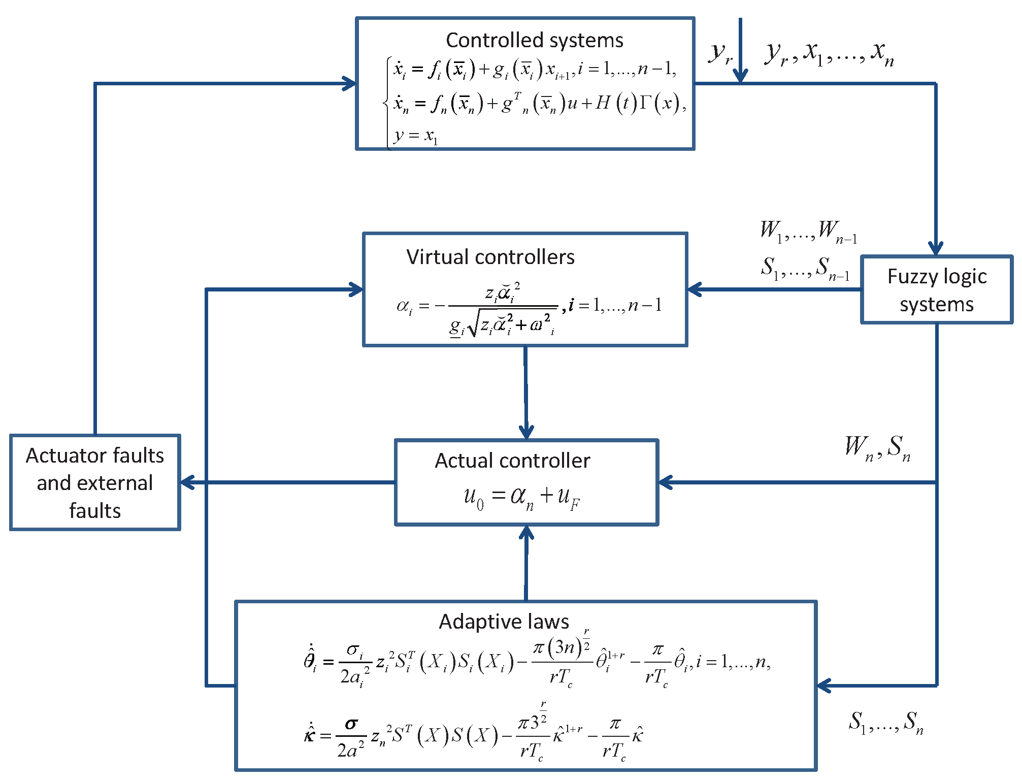
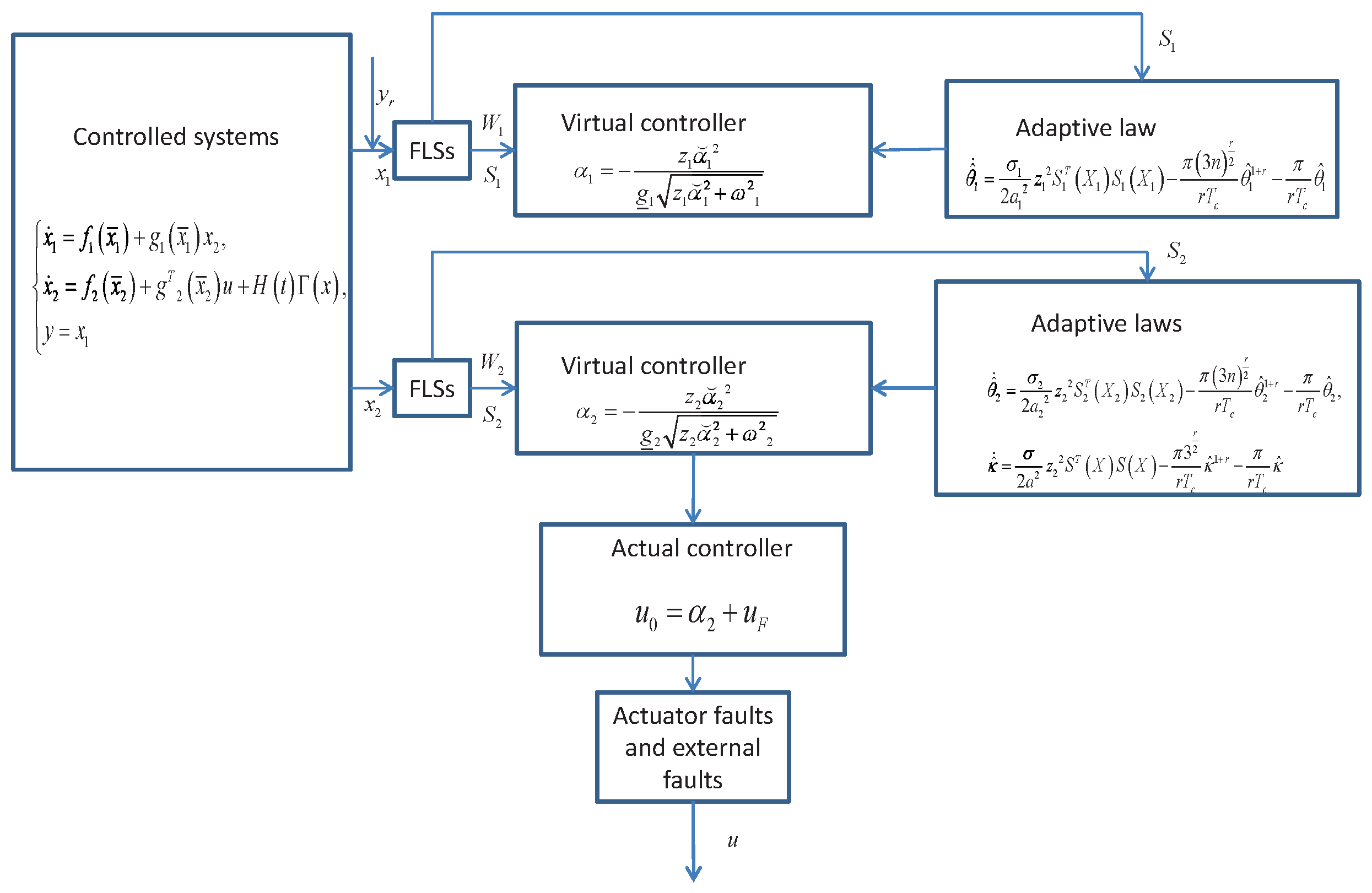
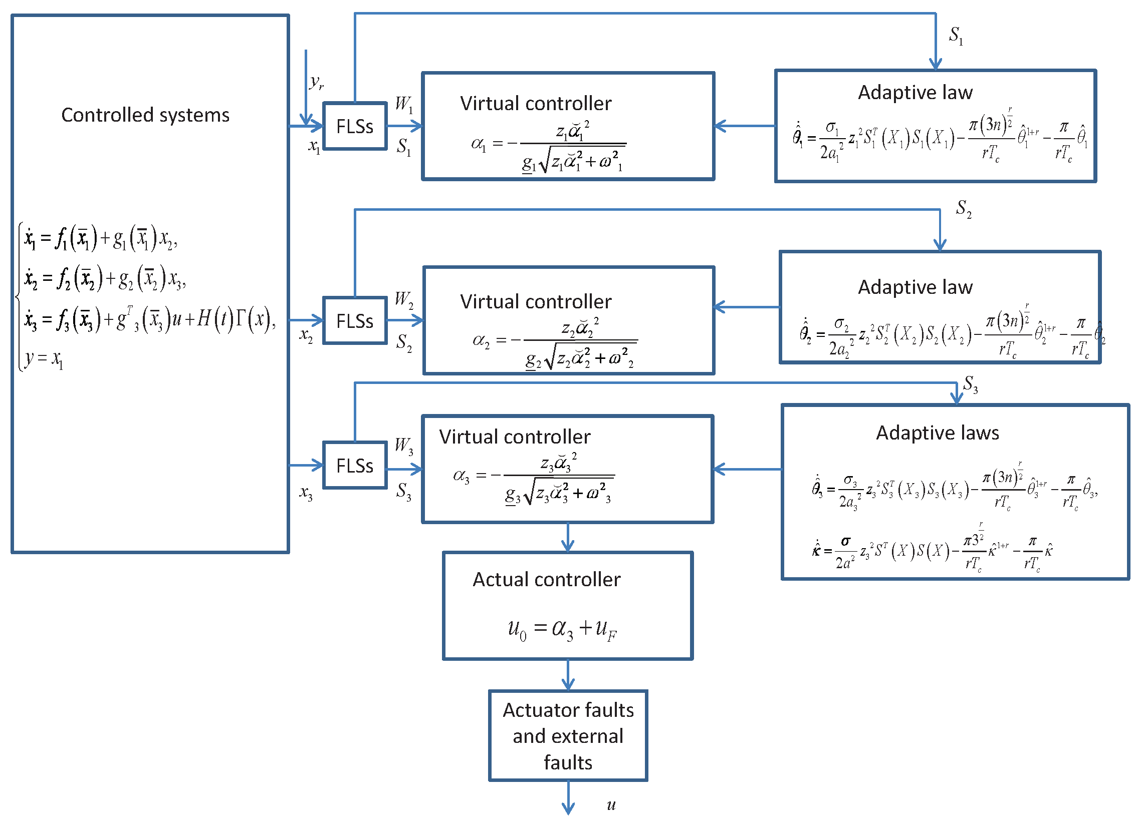
In this section, we construct a predefined-time adaptive fault-tolerant control scheme to handle nonlinear controlled systems with actuator faults and external faults; the block diagram is shown in Figure 1.

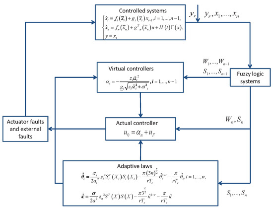
Figure 1. The block diagram of the predefined time adaptive fuzzy controller.

Firstly, we set up the following coordinate transformations:

$$\left\{\begin{array}{c}{z}_1=x_1-y_r,\hfill \\ z_i=x_i-{\alpha }_{i-1},2\le i\le n-1\hfill \end{array}\right.$$

(19)

in which $z_i(i=1,\dots ,n)$ is the tracking error, ${\alpha }_{i-1}(i=2,\dots ,n)$ is the virtual control signal, and $y_r$ is the tracking signal. The process of controller design consists of n steps:

Step 1: Due to (1) and (19), the ${\dot{z}}_1$ is given as

$$\begin{array}{ccc}\hfill {\dot{z}}_1& =& {\dot{x}}_1-{\dot{y}}_r\hfill \\ & =& f_1\left({\overline{x}}_1\right)+g_1\left({\overline{x}}_1\right)x_2-{\dot{y}}_r\hfill \\ & =& f_1\left({\overline{x}}_1\right)+g_1\left({\overline{x}}_1\right)(z_2+{\alpha }_1)-{\dot{y}}_r.\hfill \end{array}$$

(20)

Select the following Lyapunov function

$$\begin{array}{c}\hfill V_1=\frac{1}{2}{z}_1^2+\frac{1}{2{\sigma }_1}{{\tilde{\theta }}_1}^2,\end{array}$$

(21)

in which ${\tilde{\theta }}_1={\theta }_1-{\widehat{\theta }}_1$, ${\theta }_1=\left|\right|W_1{\left|\right|}^2$ is estimated by ${\widehat{\theta }}_1>0$, and the parameter ${\sigma }_1>0$ can be designed.

Then, the differentiation of $V_1$ produces

$$\begin{array}{ccc}\hfill {\dot{V}}_1& =& z_1{\dot{z}}_1-\frac{1}{{\sigma }_1}{\tilde{\theta }}_1{\dot{\widehat{\theta }}}_1\hfill \\ & =& z_1(f_1\left({\overline{x}}_1\right)+g_1\left({\overline{x}}_1\right)(z_2+{\alpha }_1)-{\dot{y}}_r)-\frac{1}{{\sigma }_1}{\tilde{\theta }}_1{\dot{\widehat{\theta }}}_1\hfill \\ & =& z_1(F_1+g_1\left({\overline{x}}_1\right)(z_2+{\alpha }_1)-\frac{1}{2}{z}_1)-\frac{1}{{\sigma }_1}{\tilde{\theta }}_1{\dot{\widehat{\theta }}}_1,\hfill \end{array}$$

(22)

where $F_1=f_1\left({\overline{x}}_1\right)-{\dot{y}}_r+\frac{1}{2}{z}_1$.

Next, according to the definition of FLSs and Lemma 2, $W_1^T{S}_1\left(X_1\right)$ can be employed to approximate $F_1$; for ${\epsilon }_1>0$, we have

$$F_1=W_1^T{S}_1\left(X_1\right)+{\delta }_1\left(X_1\right),\left|{\delta }_1\left(X_1\right)\right|\le {\epsilon }_1,$$

(23)

where $X_1={[x_1,y_r,{\dot{y}}_r]}^T$.

Then, by employing Young’s inequality, we have

$$\begin{array}{ccc}\hfill z_1{F}_1& =& z_1\left(W_1^T{S}_1\left(X_1\right)+{\delta }_1\left(X_1\right)\right)\hfill \\ & \le & |z_1|\left(\left|\right|W_1\left|\right|\left|\right|S_1\left(X_1\right)\left|\right|+{\epsilon }_1\right)\hfill \\ & \le & \frac{1}{2a_1^2}{z}_1^2{\theta }_1{S}_1^T\left(X_1\right)S_1\left(X_1\right)+\frac{a_1^2}{2}+\frac{z_1^2}{2}+\frac{{\epsilon }_1^2}{2},\hfill \end{array}$$

(24)

where $a_1>0$ is a design parameter.

Then, substituting (24) into (22), ${\dot{V}}_1$ can be derived as

$$\begin{array}{ccc}\hfill {\dot{V}}_1& \le & \frac{1}{2a_1^2}{z}_1^2{\widehat{\theta }}_1{S}_1^T\left(X_1\right)S_1\left(X_1\right)+g_1{z}_1{z}_2+g_1{z}_1{\alpha }_1\hfill \\ & & -\frac{1}{{\sigma }_1}{\tilde{\theta }}_1\left({\dot{\widehat{\theta }}}_1-\frac{{\sigma }_1}{2a_1^2}{z}_1^2{S}_1^T\left(X_1\right)S_1\left(X_1\right)\right)+\frac{a_1^2}{2}+\frac{{\epsilon }_1^2}{2}.\hfill \end{array}$$

(25)

The virtual controller ${\alpha }_1$ and adaptive law ${\widehat{\theta }}_1$ are selected as

$$\begin{array}{c}\hfill {\alpha }_1=-\frac{z_1{\check{\alpha }}_1^2}{{\underline{g}}_1\sqrt{z_1^2{\check{\alpha }}_1^2+{\omega }_1^2}},\end{array}$$

(26)

$$\begin{array}{c}\hfill {\dot{\widehat{\theta }}}_1=\frac{{\sigma }_1}{2a_1^2}{z}_1^2{S}_1^T\left(X_1\right)S_1\left(X_1\right)-\frac{\pi {\left(3n\right)}^{\frac{r}{2}}}{r{T}_c}{\widehat{\theta }}_1^{1+r}-\frac{\pi }{r{T}_c}{\widehat{\theta }}_1,\end{array}$$

(27)

where ${\omega }_1>0$ is a small parameter and ${\check{\alpha }}_1$ is designed as

$$\begin{array}{ccc}\hfill {\check{\alpha }}_1& =& \frac{1}{2a_1^2}{z}_1{\widehat{\theta }}_1{S}_1^T\left(X_1\right)S_1\left(X_1\right)+\frac{\pi {\left(3n\right)}^{\frac{r}{2}}}{r\lambda T_c}{\left(\frac{1}{2}{z}_1^2\right)}^{1+\frac{r}{2}}+\frac{\pi }{2^{1-\frac{r}{2}}r\lambda T_c}{\Phi }_1,\hfill \end{array}$$

(28)

where

$$\begin{array}{c}\hfill {\Phi }_1=\left\{\begin{array}{c}{\left(z_1^2\right)}^{1-\frac{r}{2}},\left|z_1\right|<\lambda \hfill \\ (1+pr){\lambda }^{-3-r}{z}_1^5-pr{\lambda }^{-1-r}{z}_1^3,\left|z_1\right|\ge \lambda >0\hfill \end{array}\right.\end{array}$$

(29)

where $\lambda >0$ is predefined accuracy and $p>0$ is a constant.

According to Lemma 5 and (26), one has

$$\begin{array}{ccc}\hfill g_1{z}_1{\alpha }_1& =& -\frac{g_1{z}_1^2{\check{\alpha }}_1^2}{{\underline{g}}_1\sqrt{z_1^2{\check{\alpha }}_1^2+{\omega }_1^2}}\hfill \\ & \le & -\frac{z_1^2{\check{\alpha }}_1^2}{\sqrt{z_1^2{\check{\alpha }}_1^2+{\omega }_1^2}}\hfill \\ & \le & {\omega }_1-\left|z_1{\check{\alpha }}_1\right|\hfill \\ & \le & {\omega }_1-z_1{\check{\alpha }}_1.\hfill \end{array}$$

(30)

(1) If $|z_1|\ge \lambda$, based on (28)–(30), we can obtain

$$\begin{array}{ccc}\hfill -z_1{\check{\alpha }}_1& =& -\frac{1}{2a_1^2}{z}_1^2{\widehat{\theta }}_1{S}_1^T\left(X_1\right)S_1\left(X_1\right)-\frac{\pi {\left(3n\right)}^{\frac{r}{2}}{z}_1}{r\lambda T_c}{\left(\frac{1}{2}{z}_1^2\right)}^{1+\frac{r}{2}}-\frac{\pi z_1}{2^{1-\frac{r}{2}}r\lambda T_c}{\Phi }_1\hfill \\ & \le & -\frac{1}{2a_1^2}{z}_1^2{\widehat{\theta }}_1{S}_1^T\left(X_1\right)S_1\left(X_1\right)-\frac{\pi {\left(3n\right)}^{\frac{r}{2}}}{r{T}_c}{\left(\frac{1}{2}{z}_1^2\right)}^{1+\frac{r}{2}}\hfill \\ & & -\frac{\pi }{2^{1-\frac{r}{2}}r{T}_c}\left((1+pr){\lambda }^{-3-r}{z}_1^5-pr{\lambda }^{-1-r}{z}_1^3\right)\hfill \\ & \le & -\frac{1}{2a_1^2}{z}_1^2{\widehat{\theta }}_1{S}_1^T\left(X_1\right)S_1\left(X_1\right)-\frac{\pi {\left(3n\right)}^{\frac{r}{2}}}{r{T}_c}{\left(\frac{1}{2}{z}_1^2\right)}^{1+\frac{r}{2}}\hfill \\ & & -\frac{\pi }{2^{1-\frac{r}{2}}r{T}_c}\left((1+pr){\lambda }^{-1-r}{z}_1^3-pr{\lambda }^{-1-r}{z}_1^3\right)\hfill \\ & \le & -\frac{1}{2a_1^2}{z}_1^2{\widehat{\theta }}_1{S}_1^T\left(X_1\right)S_1\left(X_1\right)-\frac{\pi {\left(3n\right)}^{\frac{r}{2}}}{r{T}_c}{\left(\frac{1}{2}{z}_1^2\right)}^{1+\frac{r}{2}}-\frac{\pi }{2^{1-\frac{r}{2}}r{T}_c}{\lambda }^{-1-r}{z}_1^3\hfill \\ & \le & -\frac{1}{2a_1^2}{z}_1^2{\widehat{\theta }}_1{S}_1^T\left(X_1\right)S_1\left(X_1\right)-\frac{\pi {\left(3n\right)}^{\frac{r}{2}}}{r{T}_c}{\left(\frac{1}{2}{z}_1^2\right)}^{1+\frac{r}{2}}-\frac{\pi }{r{T}_c}{\left(\frac{1}{2}{z}_1^2\right)}^{1-\frac{r}{2}}.\hfill \end{array}$$

(31)

By employing Assumption 1, one can obtain

$$g_1{z}_1{z}_2\le \left|{\overline{g}}_1{z}_1{z}_2\right|.$$

(32)

Then, substituting (26), (27) and (30)–(32) into (25) yields

$$\begin{array}{ccc}\hfill {\dot{V}}_1& \le & \frac{1}{2a_1^2}{z}_1^2{\widehat{\theta }}_1{S}_1^T\left(X_1\right)S_1\left(X_1\right)+g_1{z}_1{z}_2+{\omega }_1-z_1{\check{\alpha }}_1+\frac{\pi {\left(3n\right)}^{\frac{r}{2}}}{{\sigma }_{1}r{T}_c}{\tilde{\theta }}_1{\widehat{\theta }}_1^{1+r}\hfill \\ & & +\frac{\pi }{{\sigma }_{1}r{T}_c}{\tilde{\theta }}_1{\widehat{\theta }}_1+\frac{a_1^2}{2}+\frac{{\epsilon }_1^2}{2}\hfill \\ & \le & -\frac{\pi {\left(3n\right)}^{\frac{r}{2}}}{r{T}_c}{\left(\frac{1}{2}{z}_1^2\right)}^{1+\frac{r}{2}}-\frac{\pi }{r{T}_c}{\left(\frac{1}{2}{z}_1^2\right)}^{1-\frac{r}{2}}+\frac{\pi {\left(3n\right)}^{\frac{r}{2}}}{{\sigma }_{1}r{T}_c}{\tilde{\theta }}_1{\widehat{\theta }}_1^{1+r}\hfill \\ & & +\frac{\pi }{{\sigma }_{1}r{T}_c}{\tilde{\theta }}_1{\widehat{\theta }}_1+\left|{\overline{g}}_1{z}_1{z}_2\right|+b_1,\hfill \end{array}$$

(33)

where $b_1={\omega }_1+\frac{a_1^2}{2}+\frac{{\epsilon }_1^2}{2}$.

(2) If $|z_1| <\lambda$, the tracking error $z_1$ enters the predefined neighborhood, achieved the control, and from (28)–(30), one has

$$\begin{array}{ccc}\hfill -z_1{\check{\alpha }}_1& =& -\frac{1}{2a_1^2}{z}_1^2{\widehat{\theta }}_1{S}_1^T\left(X_1\right)S_1\left(X_1\right)-\frac{\pi {\left(3n\right)}^{\frac{r}{2}}{z}_1}{r\lambda T_c}{\left(\frac{1}{2}{z}_1^2\right)}^{1+\frac{r}{2}}-\frac{\pi z_1}{2^{1-\frac{r}{2}}r\lambda T_c}{\Phi }_1\hfill \\ & \le & -\frac{1}{2a_1^2}{z}_1^2{\widehat{\theta }}_1{S}_1^T\left(X_1\right)S_1\left(X_1\right)-\frac{\pi {\left(3n\right)}^{\frac{r}{2}}}{r{T}_c}{\left(\frac{1}{2}{z}_1^2\right)}^{1+\frac{r}{2}}-\frac{\pi }{r{T}_c}{\left(\frac{1}{2}{z}_1^2\right)}^{1-\frac{r}{2}},\hfill \end{array}$$

(34)

we can see that the final derivation result of (34) is the same as that of (31). Therefore, for $|z_1| \ge \lambda$ and $|z_1| <\lambda$, we always have the following inequality that holds

$$\begin{array}{ccc}\hfill {\dot{V}}_1& \le & -\frac{\pi {\left(3n\right)}^{\frac{r}{2}}}{r{T}_c}{\left(\frac{1}{2}{z}_1^2\right)}^{1+\frac{r}{2}}-\frac{\pi }{r{T}_c}{\left(\frac{1}{2}{z}_1^2\right)}^{1-\frac{r}{2}}+\frac{\pi {\left(3n\right)}^{\frac{r}{2}}}{{\sigma }_{1}r{T}_c}{\tilde{\theta }}_1{\widehat{\theta }}_1^{1+r}+\frac{\pi }{{\sigma }_{1}r{T}_c}{\tilde{\theta }}_1{\widehat{\theta }}_1\hfill \\ & & +|{\overline{g}}_1{z}_1{z}_2|+b_1.\hfill \end{array}$$

(35)

Step i $(i=2,\dots ,n-1)$: From (1) and (19), ${\dot{z}}_i$ is

$$\begin{array}{ccc}\hfill {\dot{z}}_i& =& {\dot{x}}_i-{\dot{\alpha }}_{i-1}\hfill \\ & =& f_i\left({\overline{x}}_i\right)+g_i\left({\overline{x}}_i\right)x_{i+1}-{\dot{\alpha }}_{i-1}\hfill \\ & =& f_i\left({\overline{x}}_i\right)+g_i\left({\overline{x}}_i\right)(z_{i+1}+{\alpha }_i)-{\dot{\alpha }}_{i-1}.\hfill \end{array}$$

(36)

Consider the Lyapunov function as follows:

$$V_i=V_{i-1}+\frac{1}{2}{z}_i^2+\frac{1}{2{\sigma }_i}{{\tilde{\theta }}_i}^2,$$

(37)

in which ${\tilde{\theta }}_i={\theta }_i-{\widehat{\theta }}_i$, ${\theta }_i=\left|\right|W_i{\left|\right|}^2$ is estimated by ${\widehat{\theta }}_i>0$, and the parameter ${\sigma }_i>0$ can be designed.

Then, we can obtain ${\dot{V}}_i$ as

$$\begin{array}{ccc}\hfill {\dot{V}}_i& =& {\dot{V}}_{i-1}+z_i{\dot{z}}_i-\frac{1}{{\sigma }_i}{\tilde{\theta }}_i{\dot{\widehat{\theta }}}_i\hfill \\ & =& {\dot{V}}_{i-1}+z_i\left(f_i\left({\overline{x}}_i\right)+g_i(z_{i+1}+{\alpha }_i)-{\dot{\alpha }}_{i-1}\right)-\frac{1}{{\sigma }_i}{\tilde{\theta }}_i{\dot{\widehat{\theta }}}_i\hfill \\ & =& {\dot{V}}_{i-1}+z_i\left(F_i+g_i(z_{i+1}+{\alpha }_i)-\frac{1}{2}{z}_i\right)-\frac{1}{{\sigma }_i}{\tilde{\theta }}_i{\dot{\widehat{\theta }}}_i,\hfill \end{array}$$

(38)

where $F_i=f_i\left({\overline{x}}_i\right)-{\dot{\alpha }}_{i-1}+\frac{1}{2}{z}_i$.

Next, the FLSs $W^T{S}_i\left(X_i\right)$ are exploited to model $F_i$, and one can yield

$$F_i=W_i^T{S}_i\left(X_i\right)+{\delta }_i\left(X_i\right),\left|{\delta }_i\left(X_i\right)\right|\le {\epsilon }_i,$$

(39)

where ${\epsilon }_i>0$ is given, $X_i={[x_1,\dots ,x_i,y_r,{\dot{y}}_r,\dots ,y_r^{\left(i\right)}]}^T$.

Then, by utilizing Young’s inequality, we can obtain

$$\begin{array}{ccc}\hfill z_i{F}_i& =& z_i\left(W_i^T{S}_i\left(X_i\right)+{\delta }_i\left(X_i\right)\right)\hfill \\ & \le & |z_i|\left(\left|\right|W_i\left|\right|\left|\right|S_i\left(X_i\right)\left|\right|+{\epsilon }_i\right)\hfill \\ & \le & \frac{1}{2a_i^2}{z}_i^2{\theta }_i{S}_i^T\left(X_i\right)S_i\left(X_i\right)+\frac{a_i^2}{2}+\frac{z_i^2}{2}+\frac{{\epsilon }_i^2}{2},\hfill \end{array}$$

(40)

where $a_i>0$ is a constant.

Substituting (40) into (38), one has

$$\begin{array}{ccc}\hfill {\dot{V}}_i& \le & {\dot{V}}_{i-1}+\frac{1}{2a_i^2}{z}_i^2{\widehat{\theta }}_i{S}_i^T\left(X_i\right)S_i\left(X_i\right)+g_i{z}_i{z}_{i+1}+g_i{z}_i{\alpha }_i\hfill \\ & & -\frac{1}{{\sigma }_i}{\tilde{\theta }}_i\left(\dot{{\widehat{\theta }}_i}-\frac{{\sigma }_i}{2a_i^2}{z}_i^2{S}_i^T\left(X_i\right)S_i\left(X_i\right)\right)+\frac{a_i^2}{2}+\frac{{\epsilon }_i^2}{2}.\hfill \end{array}$$

(41)

Choose the virtual controller ${\alpha }_i$ and adaptive law ${\widehat{\theta }}_i$ as

$$\begin{array}{cc}\hfill {\alpha }_i& =-\frac{1}{{\underline{g}}_i}\left(\frac{z_i{\check{\alpha }}_i^2}{\sqrt{z_i^2{\check{\alpha }}_i^2+{\omega }_i^2}}+\frac{z_{i-1}^2{\overline{g}}_{i-1}^2{z}_i}{\sqrt{z_{i-1}^2{\overline{g}}_{i-1}^2{z}_i^2+{\omega }_i^2}}\right),\end{array}$$

(42)

$${\dot{\widehat{\theta }}}_i=\frac{{\sigma }_i}{2a_i^2}{z}_i^2{S}_i^T\left(X_i\right)S_i\left(X_i\right)-\frac{\pi {\left(3n\right)}^{\frac{r}{2}}}{r{T}_c}{\widehat{\theta }}_i^{1+r}-\frac{\pi }{r{T}_c}{\widehat{\theta }}_i,$$

(43)

in which ${\omega }_i>0$ is a small parameter and ${\check{\alpha }}_i$ is designed as

$$\begin{array}{ccc}\hfill {\check{\alpha }}_i& =& \frac{1}{2a_i^2}{z}_i{\widehat{\theta }}_i{S}_i^T\left(X_i\right)S_i\left(X_i\right)+\frac{\pi {\left(3n\right)}^{\frac{r}{2}}}{r\lambda T_c}{\left(\frac{1}{2}{z}_i^2\right)}^{1+\frac{r}{2}}+\frac{\pi }{2^{1-\frac{r}{2}}r\lambda T_c}{\Phi }_i,\hfill \end{array}$$

(44)

where

$$\begin{array}{c}\hfill {\Phi }_i=\left\{\begin{array}{c}{\left(z_i^2\right)}^{1-\frac{r}{2}},\left|z_i\right|<\lambda \hfill \\ (1+pr){\lambda }^{-3-r}{z}_i^5-pr{\lambda }^{-1-r}{z}_i^3,\left|z_i\right|\ge \lambda >0\hfill \end{array}\right.\end{array}$$

(45)

According to Lemma 5 and (42), we have

$$\begin{array}{ccc}\hfill g_i{z}_i{\alpha }_i& =& -\frac{g_i{z}_i^2{\check{\alpha }}_i^2}{{\underline{g}}_i\sqrt{z_i^2{\check{\alpha }}_i^2+{\omega }_i^2}}-\frac{g_i{z}_{i-1}^2{\overline{g}}_{i-1}^2{z}_i^2}{{\underline{g}}_i\sqrt{z_{i-1}^2{\overline{g}}_{i-1}^2{z}_i^2+{\omega }_i^2}}\hfill \\ & \le & 2{\omega }_i-|z_i{\check{\alpha }}_i|-|{\overline{g}}_{i-1}{z}_{i-1}{z}_i|\hfill \\ & \le & 2{\omega }_i-z_i{\check{\alpha }}_i-\left|{\overline{g}}_{i-1}{z}_{i-1}{z}_i\right|.\hfill \end{array}$$

(46)

(1) If $|z_i|\ge \lambda >0$, from (44)–(46) and similar to (31), one has

$$\begin{array}{ccc}\hfill -z_i{\check{\alpha }}_i& =& -\frac{1}{2a_i^2}{z}_i^2{\widehat{\theta }}_i{S}_i^T\left(X_i\right)S_i\left(X_i\right)-\frac{\pi {\left(3n\right)}^{\frac{r}{2}}{z}_i}{r\lambda T_c}{\left(\frac{1}{2}{z}_i^2\right)}^{1+\frac{r}{2}}-\frac{\pi z_i}{2^{1-\frac{r}{2}}r\lambda T_c}{\Phi }_i\hfill \\ & \le & -\frac{1}{2a_i^2}{z}_i^2{\widehat{\theta }}_i{S}_i^T\left(X_i\right)S_i\left(X_i\right)-\frac{\pi {\left(3n\right)}^{\frac{r}{2}}}{r{T}_c}{\left(\frac{1}{2}{z}_i^2\right)}^{1+\frac{r}{2}}-\frac{\pi }{r{T}_c}{\left(\frac{1}{2}{z}_i^2\right)}^{1-\frac{r}{2}}.\hfill \end{array}$$

(47)

By utilizing Assumption 1, we can obtain

$$g_i{z}_i{z}_{i+1}\le \left|{\overline{g}}_i{z}_i{z}_{i+1}\right|.$$

(48)

Then, bringing (42), (43) and (46)–(48) into (41), one has

$$\begin{array}{ccc}\hfill {\dot{V}}_i& \le & {\dot{V}}_{i-1}+\frac{1}{2a_i^2}{z}_i^2{\widehat{\theta }}_i{S}_i^T\left(X_i\right)S_i\left(X_i\right)+g_i{z}_i{z}_{i+1}+2{\omega }_i-z_i{\check{\alpha }}_i-\left|{\overline{g}}_{i-1}{z}_{i-1}{z}_i\right|\hfill \\ & & +\frac{\pi {\left(3n\right)}^{\frac{r}{2}}}{{\sigma }_{i}r{T}_c}{\tilde{\theta }}_i{\widehat{\theta }}_i^{1+r}+\frac{\pi }{{\sigma }_{i}r{T}_c}{\tilde{\theta }}_i{\widehat{\theta }}_i+\frac{a_i^2}{2}+\frac{{\epsilon }_i^2}{2}\hfill \\ & \le & -\sum _{j=1}^{i-1}\frac{\pi {\left(3n\right)}^{\frac{r}{2}}}{r{T}_c}{\left(\frac{1}{2}{z}_j^2\right)}^{1+\frac{r}{2}}-\sum _{j=1}^{i-1}\frac{\pi }{r{T}_c}{\left(\frac{1}{2}{z}_j^2\right)}^{1-\frac{r}{2}}+\sum _{j=1}^{i-1}\frac{\pi {\left(3n\right)}^{\frac{r}{2}}}{{\sigma }_{j}r{T}_c}{\tilde{\theta }}_j{\widehat{\theta }}_j^{1+r}\hfill \\ & & +\sum _{j=1}^{i-1}\frac{\pi }{{\sigma }_{j}r{T}_c}{\tilde{\theta }}_j{\widehat{\theta }}_j+\left|{\overline{g}}_{-1}{z}_{i-1}{z}_i\right|-\frac{\pi {\left(3n\right)}^{\frac{r}{2}}}{r{T}_c}{\left(\frac{1}{2}{z}_i^2\right)}^{1+\frac{r}{2}}+b_{i-1}-\frac{\pi }{r{T}_c}{\left(\frac{1}{2}{z}_i^2\right)}^{1-\frac{r}{2}}\hfill \\ & & +\frac{\pi {\left(3n\right)}^{\frac{r}{2}}}{{\sigma }_{i}r{T}_c}{\tilde{\theta }}_i{\widehat{\theta }}_i^{1+r}+\frac{\pi }{{\sigma }_{i}r{T}_c}{\tilde{\theta }}_i{\widehat{\theta }}_i+|{\overline{g}}_i{z}_i{z}_{i+1}|-|{\overline{g}}_{i-1}{z}_{i-1}{z}_i|+\frac{a_i^2}{2}+\frac{{\epsilon }_i^2}{2}+2{\omega }_i\hfill \\ & \le & -\sum _{j=1}^i\frac{\pi {\left(3n\right)}^{\frac{r}{2}}}{r{T}_c}{\left(\frac{1}{2}{z}_j^2\right)}^{1+\frac{r}{2}}-\sum _{j=1}^i\frac{\pi }{r{T}_c}{\left(\frac{1}{2}{z}_j^2\right)}^{1-\frac{r}{2}}+\sum _{j=1}^i\frac{\pi {\left(3n\right)}^{\frac{r}{2}}}{{\sigma }_{j}r{T}_c}{\tilde{\theta }}_j{\widehat{\theta }}_j^{1+r}\hfill \\ & & +\sum _{j=1}^i\frac{\pi }{{\sigma }_{j}r{T}_c}{\tilde{\theta }}_j{\widehat{\theta }}_j+\left|{\overline{g}}_i{z}_i{z}_{i+1}\right|+b_i,\hfill \end{array}$$

(49)

where $b_i=b_{i-1}+\frac{a_i^2}{2}+\frac{{\epsilon }_i^2}{2}+2{\omega }_i$.

(2) If $|z_i| <\lambda$, according to (44)–(46), we can obtain

$$\begin{array}{ccc}\hfill -z_i{\check{\alpha }}_i& =& -\frac{1}{2a_i^2}{z}_i^2{\widehat{\theta }}_i{S}_i^T\left(X_i\right)S_i\left(X_i\right)-\frac{\pi {\left(3n\right)}^{\frac{r}{2}}{z}_i}{r\lambda T_c}{\left(\frac{1}{2}{z}_i^2\right)}^{1+\frac{r}{2}}-\frac{\pi z_i}{2^{1-\frac{r}{2}}r\lambda T_c}{\Phi }_i\hfill \\ & \le & -\frac{1}{2a_i^2}{z}_i^2{\widehat{\theta }}_i{S}_i^T\left(X_i\right)S_i\left(X_i\right)-\frac{\pi {\left(3n\right)}^{\frac{r}{2}}}{r{T}_c}{\left(\frac{1}{2}{z}_i^2\right)}^{1+\frac{r}{2}}-\frac{\pi }{r{T}_c}{\left(\frac{1}{2}{z}_i^2\right)}^{1-\frac{r}{2}},\hfill \end{array}$$

(50)

the inequality (50) is the same as inequality (47).

Therefore, based on the above derivation of situation (1) and situation (2), one has

$$\begin{array}{ccc}\hfill {\dot{V}}_i& \le & -\sum _{j=1}^i\frac{\pi {\left(3n\right)}^{\frac{r}{2}}}{r{T}_c}{\left(\frac{1}{2}{z}_j^2\right)}^{1+\frac{r}{2}}-\sum _{j=1}^i\frac{\pi }{r{T}_c}{\left(\frac{1}{2}{z}_j^2\right)}^{1-\frac{r}{2}}+\sum _{j=1}^i\frac{\pi {\left(3n\right)}^{\frac{r}{2}}}{{\sigma }_{j}r{T}_c}{\tilde{\theta }}_j{\widehat{\theta }}_j^{1+r}\hfill \\ & & +\sum _{j=1}^i\frac{\pi }{{\sigma }_{j}r{T}_c}{\tilde{\theta }}_j{\widehat{\theta }}_j+\left|{\overline{g}}_i{z}_i{z}_{i+1}\right|+b_i.\hfill \end{array}$$

(51)

Step n: The controller will be presented in this step. Similar to Step i, one can obtain ${\dot{z}}_n$:

$$\begin{array}{ccc}\hfill {\dot{z}}_n& =& {\dot{x}}_n-{\dot{\alpha }}_{n-1}\hfill \\ & =& f_n\left({\overline{x}}_n\right)+g_n^{T}u+H\left(t\right)\Gamma \left(x\right)-{\dot{\alpha }}_{n-1}.\hfill \end{array}$$

(52)

From (6) and (8), we have

$$\begin{array}{ccc}\hfill g_n^{T}u& =& g_n^T\left(\rho \nu \left(t\right)+\zeta (\underline{u}-\rho \nu \left(t\right))\right)\hfill \\ & =& g_n^T\left((1-\zeta )\rho \nu \left(t\right)+\zeta \underline{u}\right)\hfill \\ & =& \sum _{j\ne j_1,\dots ,j_p}{\rho }_j{g}_{nj}{\eta }_j{u}_0+\sum _{j=j_1,\dots ,j_p}{g}_{nj}{\underline{u}}_j\hfill \\ & =& g_f{u}_0+u_f,\hfill \end{array}$$

(53)

where $g_f={\displaystyle \sum _{j\ne j_1,\dots ,j_p}}{\rho }_j{g}_{nj}{\eta }_j$ and $u_f={\displaystyle \sum _{j=j_1,\dots ,j_p}}{g}_{nj}{\underline{u}}_j$.

The Lyapunov function candidate function is chosen as shown below:

$$V_n=V_{n-1}+\frac{1}{2}{z}_n^2+\frac{1}{2{\sigma }_n}{{\tilde{\theta }}_n}^2+\frac{1}{2\sigma }{\tilde{\kappa }}^2,$$

(54)

where ${\tilde{\theta }}_n={\theta }_n-{\widehat{\theta }}_n$, $\tilde{\kappa }=\kappa -\widehat{\kappa }$; ${\theta }_n=\left|\right|W_n{\left|\right|}^2$ and $\kappa ={\left|\right|W\left|\right|}^2$ are estimated by ${\widehat{\theta }}_i>0$ and $\widehat{\kappa }>0$; the parameters ${\sigma }_i>0$ and $\sigma >0$ can be designed.

Then, the time differentiation of $V_n$ is

$$\begin{array}{ccc}\hfill \dot{V_n}& =& {\dot{V}}_{n-1}+z_n{\dot{z}}_n-\frac{1}{{\sigma }_n}{\tilde{\theta }}_n{\dot{\widehat{\theta }}}_n-\frac{1}{\sigma }\tilde{\kappa }\dot{\widehat{\kappa }}\hfill \\ & =& {\dot{V}}_{n-1}+z_n(f_n\left({\overline{x}}_n\right)+g_f{u}_0+u_f+H\left(t\right)\Gamma \left(x\right)-{\dot{\alpha }}_{n-1})-\frac{1}{{\sigma }_n}{\tilde{\theta }}_n{\dot{\widehat{\theta }}}_n-\frac{1}{\sigma }\tilde{\kappa }\dot{\widehat{\kappa }}\hfill \\ & =& {\dot{V}}_{n-1}+z_n\left(F_n+g_f{u}_0+u_f+H\left(t\right)\Gamma \left(x\right)-z_n\right)-\frac{1}{{\sigma }_n}{\tilde{\theta }}_n{\dot{\widehat{\theta }}}_n-\frac{1}{\sigma }\tilde{\kappa }\dot{\widehat{\kappa }},\hfill \end{array}$$

(55)

where $F_n=f_n\left({\overline{x}}_n\right)-{\dot{\alpha }}_{n-1}+z_n$.

Then, based on FLSs and Lemma 2, $W_n^T{S}_n\left(X_n\right)$ and ${\Phi }^{T}S\left(X\right)$ are used to model $F_n$ and $\Gamma \left(x\right)$, respectively. For the given ${\epsilon }_n>0$ and $\overline{\delta }>0$, we have

$$F_n=W_n^T{S}_n\left(X_n\right)+{\delta }_n\left(X_n\right),\left|{\delta }_n\left(X_n\right)\right|\le {\epsilon }_n,$$

(56)

$$\Gamma \left(x\right)={\Phi }^{T}S\left(X\right)+\delta \left(X\right),\left|\delta \left(X\right)\right|\le \overline{\delta },$$

(57)

where $X_n={[x_1,\dots ,x_n,y_r,{\dot{y}}_r,\dots ,y_r^{\left(n\right)}]}^T$, $X={[x_1,x_2,\dots ,x_n]}^T$.

Then, by utilizing Young’s inequality, it can be obtained that

$$\begin{array}{ccc}\hfill z_n{F}_n& \le & \frac{1}{2a_n^2}{z}_n^2{\theta }_n{S}_n^T\left(X_n\right)S_n\left(X_n\right)+\frac{a_n^2}{2}+\frac{z_n^2}{2}+\frac{{\epsilon }_n^2}{2},\hfill \end{array}$$

(58)

$$\begin{array}{ccc}\hfill z_{n}H\left(t\right)\Gamma \left(x\right)& \le & \frac{1}{2a^2}{z}_n^2\kappa S^T\left(X\right)S\left(X\right)+\frac{a^2}{2}+\frac{z_n^2}{2}+\frac{{\overline{\delta }}^2}{2},\hfill \end{array}$$

(59)

where $a_n>0$ and $a>0$ are design constants.

Next, bringing (58) and (59) into (55), one can obtain

$$\begin{array}{ccc}\hfill \dot{V_n}& \le & {\dot{V}}_{n-1}+\frac{1}{2a_n^2}{z}_n^2{\widehat{\theta }}_n{S}_n^T\left(X_n\right)S_n\left(X_n\right)+\frac{1}{2a^2}{z}_n^2\widehat{\kappa }{S}^T\left(X\right)S\left(X\right)+z_n\left(g_f{u}_0+u_f\right)\hfill \\ & & -\frac{1}{{\sigma }_n}{\tilde{\theta }}_n\left({\dot{\widehat{\theta }}}_n-\frac{{\sigma }_n}{2a_n^2}{z}_n^2{S}_n^T\left(X_n\right)S_n\left(X_n\right)\right)-\frac{1}{\sigma }\tilde{\kappa }\left(\dot{\widehat{\kappa }}-\frac{\sigma }{2a^2}{z}_n^2{S}^T\left(X\right)S\left(X\right)\right)\hfill \\ & & +\frac{a_n^2}{2}+\frac{{\epsilon }_n^2}{2}+\frac{a^2}{2}+\frac{{\overline{\delta }}^2}{2}.\hfill \end{array}$$

(60)

We define the control law as

$$u_0={\alpha }_n+u_F,$$

(61)

in which

$$\begin{array}{ccc}\hfill {\alpha }_n& =& -\frac{1}{g_f}\left(\frac{z_n{\check{\alpha }}_n^2}{\sqrt{z_n^2{\check{\alpha }}_n^2+{\omega }_n^2}}+\frac{z_{n-1}^2{\overline{g}}_{n-1}^2{z}_n}{\sqrt{z_{n-1}^2{\overline{g}}_{n-1}^2{z}_n^2+{\omega }_n^2}}\right)-\frac{1}{g_f}{u}_f,\hfill \end{array}$$

(62)

$$u_F=-\frac{1}{2g_f{a}^2}\widehat{\kappa }{z}_n{S}^T\left(X\right)S\left(X\right),$$

(63)

where ${\omega }_n>0$ is a small parameter and ${\check{\alpha }}_n$ is selected as

$$\begin{array}{ccc}\hfill {\check{\alpha }}_n& =& \frac{1}{2a_n^2}{z}_n{\widehat{\theta }}_n{S}_n^T\left(X_n\right)S_n\left(X_n\right)+\frac{\pi {\left(3n\right)}^{\frac{r}{2}}}{r\lambda T_c}{\left(\frac{1}{2}{z}_n^2\right)}^{1+\frac{r}{2}}+\frac{\pi }{2^{1-\frac{r}{2}}r\lambda T_c}{\Phi }_n,\hfill \end{array}$$

(64)

where ${\Phi }_n$ is designed as

$$\begin{array}{c}\hfill {\Phi }_n=\left\{\begin{array}{c}{\left(z_n^2\right)}^{1-\frac{r}{2}},\left|z_n\right|<\lambda \hfill \\ (1+pr){\lambda }^{-3-r}{z}_n^5-pr{\lambda }^{-1-r}{z}_n^3,\left|z_n\right|\ge \lambda >0\hfill \end{array}\right.\end{array}$$

(65)

The adaptive law ${\widehat{\theta }}_n$ and $\widehat{\kappa }$ are constructed separately as

$${\dot{\widehat{\theta }}}_n=\frac{{\sigma }_n}{2a_n^2}{z}_n^2{S}_n^T\left(X_n\right)S_n\left(X_n\right)-\frac{\pi {\left(3n\right)}^{\frac{r}{2}}}{r{T}_c}{\widehat{\theta }}_n^{1+r}-\frac{\pi }{r{T}_c}{\widehat{\theta }}_n,$$

(66)

$$\dot{\widehat{\kappa }}=\frac{\sigma }{2a^2}{z}_n^2{S}^T\left(X\right)S\left(X\right)-\frac{\pi 3^{\frac{r}{2}}}{r{T}_c}{\widehat{\kappa }}^{1+r}-\frac{\pi }{r{T}_c}\widehat{\kappa }.$$

(67)

According to (62), (63) and Lemma 5, we have

$$\begin{array}{ccc}\hfill z_n{g}_f{\alpha }_n& \le & -\frac{z_n^2{\check{\alpha }}_n^2}{\sqrt{z_n^2{\check{\alpha }}_n^2+{\omega }_n^2}}-\frac{z_{n-1}^2{\overline{g}}_{n-1}^2{z}_n^2}{\sqrt{z_{n-1}^2{\overline{g}}_{n-1}^2{z}_n^2+{\omega }_n^2}}-z_n{u}_f\hfill \\ & \le & 2{\omega }_n-|z_n{\check{\alpha }}_n|-|{\overline{g}}_{n-1}{z}_{n-1}{z}_n|-z_n{u}_f\hfill \\ & \le & 2{\omega }_n-z_n{\check{\alpha }}_n-\left|{\overline{g}}_{n-1}{z}_{n-1}{z}_n\right|-z_n{u}_f,\hfill \end{array}$$

(68)

$$z_n{g}_f{u}_F\le -\frac{1}{2a^2}\widehat{\kappa }{z}_n^2{S}^T\left(X\right)S\left(X\right).$$

(69)

Similar to Step i, when $|z_n|\ge \lambda >0$ or $|z_n|<\lambda$, substituting (64)–(69) into (60) yields

$$\begin{array}{ccc}\hfill \dot{V_n}& \le & {\dot{V}}_{n-1}+\frac{1}{2a_n^2}{z}_n^2{\widehat{\theta }}_n{S}_n^T\left(X_n\right)S_n\left(X_n\right)+2{\omega }_n-z_n{\check{\alpha }}_n+\frac{1}{2a^2}{z}_n^2\widehat{\kappa }{S}^T\left(X\right)S\left(X\right)\hfill \\ & & -|{\overline{g}}_{n-1}{z}_{n-1}{z}_n|+z_n{g}_f{u}_F+\frac{\pi {\left(3n\right)}^{\frac{r}{2}}}{{\sigma }_{n}r{T}_c}{\tilde{\theta }}_n{\widehat{\theta }}_n^{1+r}+\frac{\pi }{{\sigma }_{n}r{T}_c}{\tilde{\theta }}_n{\widehat{\theta }}_n+\frac{\pi 3^{\frac{r}{2}}}{\sigma r{T}_c}\tilde{\kappa }{\widehat{\kappa }}^{1+r}\hfill \\ & & +\frac{\pi }{\sigma r{T}_c}\tilde{\kappa }\widehat{\kappa }+\frac{1}{2}{a}_n^2+\frac{1}{2}{\epsilon }_n^2+\frac{1}{2}{a}^2+\frac{1}{2}{\overline{\delta }}^2\hfill \\ & \le & -\sum _{j=1}^{n-1}\frac{\pi {\left(3n\right)}^{\frac{r}{2}}}{r{T}_c}{\left(\frac{1}{2}{z}_j^2\right)}^{1+\frac{r}{2}}-\sum _{j=1}^{n-1}\frac{\pi }{r{T}_c}{\left(\frac{1}{2}{z}_j^2\right)}^{1-\frac{r}{2}}+\sum _{j=1}^{n-1}\frac{\pi {\left(3n\right)}^{\frac{r}{2}}}{{\sigma }_{j}r{T}_c}{\tilde{\theta }}_j{\widehat{\theta }}_j^{1+r}+\sum _{j=1}^{n-1}\frac{\pi }{{\sigma }_{j}r{T}_c}{\tilde{\theta }}_j{\widehat{\theta }}_j\hfill \\ & & +|{\overline{g}}_{n-1}{z}_{n-1}{z}_n|+b_{n-1}-\frac{\pi {\left(3n\right)}^{\frac{r}{2}}}{r{T}_c}{\left(\frac{1}{2}{z}_n^2\right)}^{1+\frac{r}{2}}-\frac{\pi }{r{T}_c}{\left(\frac{1}{2}{z}_n^2\right)}^{1-\frac{r}{2}}-\left|{\overline{g}}_{n-1}{z}_{n-1}{z}_n\right|\hfill \\ & & +\frac{\pi {\left(3n\right)}^{\frac{r}{2}}}{{\sigma }_{n}r{T}_c}{\tilde{\theta }}_n{\widehat{\theta }}_n^{1+r}+\frac{\pi }{{\sigma }_{n}r{T}_c}{\tilde{\theta }}_n{\widehat{\theta }}_n+\frac{\pi 3^{\frac{r}{2}}}{\sigma r{T}_c}\tilde{\kappa }{\widehat{\kappa }}^{1+r}+\frac{\pi }{\sigma r{T}_c}\tilde{\kappa }\widehat{\kappa }+\frac{a_n^2}{2}+\frac{{\epsilon }_n^2}{2}+\frac{a^2}{2}+\frac{{\overline{\delta }}^2}{2}+2{\omega }_n\hfill \\ & \le & -\sum _{j=1}^n\frac{\pi {\left(3n\right)}^{\frac{r}{2}}}{r{T}_c}{\left(\frac{1}{2}{z}_j^2\right)}^{1+\frac{r}{2}}-\sum _{j=1}^n\frac{\pi }{r{T}_c}{\left(\frac{1}{2}{z}_j^2\right)}^{1-\frac{r}{2}}+\sum _{j=1}^n\frac{\pi {\left(3n\right)}^{\frac{r}{2}}}{{\sigma }_{j}r{T}_c}{\tilde{\theta }}_j{\widehat{\theta }}_j^{1+r}+\sum _{j=1}^n\frac{\pi }{{\sigma }_{j}r{T}_c}{\tilde{\theta }}_j{\widehat{\theta }}_j\hfill \\ & & +\frac{\pi 3^{\frac{r}{2}}}{\sigma r{T}_c}\tilde{\kappa }{\widehat{\kappa }}^{1+r}+\frac{\pi }{\sigma r{T}_c}\tilde{\kappa }\widehat{\kappa }+b_n,\hfill \end{array}$$

(70)

where $b_n=b_{n-1}+\frac{a_n^2}{2}+\frac{{\epsilon }_n^2}{2}+\frac{a^2}{2}+\frac{{\overline{\delta }}^2}{2}+2{\omega }_n$.

Theorem 1. 

For the nonlinear systems (1) with actuator faults and external faults, when the virtual control signals (26), (42), the actual control (61) and the adaptive laws (27), (43), (66) and (67) are adopted. By designing appropriate parameters, all signals defined in these closed-loop systems maintain boundedness and $z_1$ will converge to a predefined accuracy λ within a predefined time $2T_c$.

Proof of Theorem 1. 

According to Lemma 4, Lemma 7 and $0<r<1$, we can deduce that

$$\begin{array}{ccc}\hfill \sum _{j=1}^n\frac{\pi {\left(3n\right)}^{\frac{r}{2}}}{{\sigma }_{j}r{T}_c}{\tilde{\theta }}_j{\widehat{\theta }}_j^{1+r}& \le & \sum _{j=1}^n\frac{1+r}{2+r}\frac{\pi {\left(3n\right)}^{\frac{r}{2}}}{{\sigma }_{j}r{T}_c}\left({{\theta }_j}^{2+r}-{{\tilde{\theta }}_j}^{2+r}\right)\hfill \\ & \le & \sum _{j=1}^n\frac{\pi {\left(3n\right)}^{\frac{r}{2}}}{{\sigma }_{j}r{T}_c}\left({{\theta }_j}^{2+r}-{{\tilde{\theta }}_j}^{2+r}\right)\hfill \\ & \le & \sum _{j=1}^n\frac{\pi {\left(3n\right)}^{\frac{r}{2}}}{{\sigma }_{j}r{T}_c}{{\theta }_j}^{2+r}-\sum _{j=1}^n\frac{\pi 3^{\frac{r}{2}}}{r{T}_c}{\left(\frac{{{\tilde{\theta }}_j}^2}{2{\sigma }_j}\right)}^{1+\frac{r}{2}}.\hfill \end{array}$$

(71)

Similarly, it can be derived that

$$\begin{array}{ccc}\hfill \frac{\pi 3^{\frac{r}{2}}}{\sigma r{T}_c}\tilde{\kappa }{\widehat{\kappa }}^{1+r}& \le & \frac{\pi 3^{\frac{r}{2}}}{\sigma r{T}_c}{\kappa }^{2+r}-\frac{\pi 3^{\frac{r}{2}}}{r{T}_c}{\left(\frac{{\tilde{\kappa }}^2}{2\sigma }\right)}^{1+\frac{r}{2}}.\hfill \end{array}$$

(72)

By using Young’s inequality, we have

$$\begin{array}{c}\hfill {\tilde{\theta }}_j{\widehat{\theta }}_j\le \frac{1}{2}{{\theta }_j}^2-\frac{1}{2}{{\tilde{\theta }}_j}^2,\end{array}$$

(73)

$$\begin{array}{c}\hfill \tilde{\kappa }\widehat{\kappa }\le \frac{1}{2}{\kappa }^2-\frac{1}{2}{\tilde{\kappa }}^2.\end{array}$$

(74)

Substituting (71)–(74) into (70) yields

$$\begin{array}{ccc}\hfill {\dot{V}}_n& \le & -\sum _{j=1}^n\frac{\pi {\left(3n\right)}^{\frac{r}{2}}}{r{T}_c}{\left(\frac{1}{2}{z}_j^2\right)}^{1+\frac{r}{2}}-\sum _{j=1}^n\frac{\pi }{r{T}_c}{\left(\frac{1}{2}{z}_j^2\right)}^{1-\frac{r}{2}}-\sum _{j=1}^n\frac{\pi 3^{\frac{r}{2}}}{r{T}_c}{\left(\frac{{{\tilde{\theta }}_j}^2}{2{\sigma }_j}\right)}^{1+\frac{r}{2}}\hfill \\ & & -\frac{\pi 3^{\frac{r}{2}}}{r{T}_c}{\left(\frac{{\tilde{\kappa }}^2}{2\sigma }\right)}^{1+\frac{r}{2}}-\sum _{j=1}^n\frac{\pi }{2{\sigma }_{j}r{T}_c}{{\tilde{\theta }}_j}^2-\frac{\pi }{2\sigma r{T}_c}{\tilde{\kappa }}^2+\frac{\pi }{r{T}_c}{\left(\sum _{j=1}^n\frac{{{\tilde{\theta }}_j}^2}{2{\sigma }_j}\right)}^{1-\frac{r}{2}}\hfill \\ & & -\frac{\pi }{r{T}_c}{\left(\sum _{j=1}^n\frac{{{\tilde{\theta }}_j}^2}{2{\sigma }_j}\right)}^{1-\frac{r}{2}}+\frac{\pi }{r{T}_c}{\left(\frac{{\tilde{\kappa }}^2}{2\sigma }\right)}^{1-\frac{r}{2}}-\frac{\pi }{r{T}_c}{\left(\frac{{\tilde{\kappa }}^2}{2\sigma }\right)}^{1-\frac{r}{2}}+\sum _{j=1}^n\frac{\pi {\left(3n\right)}^{\frac{r}{2}}}{{\sigma }_{j}r{T}_c}{{\theta }_j}^{2+r}\hfill \\ & & +\frac{\pi 3^{\frac{r}{2}}}{\sigma r{T}_c}{\kappa }^{2+r}+\sum _{j=1}^n\frac{\pi }{2{\sigma }_{j}r{T}_c}{\theta }_j^2+\frac{\pi }{2\sigma r{T}_c}{\kappa }^2+b_n.\hfill \end{array}$$

(75)

By using Lemma 6, one can obtain

$$\begin{array}{c}\hfill \frac{\pi }{r{T}_c}{\left(\sum _{j=1}^n\frac{{{\tilde{\theta }}_j}^2}{2{\sigma }_j}\right)}^{1-\frac{r}{2}}\le \frac{\pi }{r{T}_c}\sum _{j=1}^n\frac{{{\tilde{\theta }}_j}^2}{2{\sigma }_j}+\frac{\pi }{2T_c}{\left(\frac{2}{2-r}\right)}^{\frac{r-2}{r}},\end{array}$$

(76)

$$\begin{array}{c}\hfill \frac{\pi }{r{T}_c}{\left(\frac{{\tilde{\eta }}^2}{2\sigma }\right)}^{1-\frac{r}{2}}\le \frac{\pi }{r{T}_c}\frac{{\tilde{\kappa }}^2}{2\sigma }+\frac{\pi }{2T_c}{\left(\frac{2}{2-r}\right)}^{\frac{r-2}{r}}.\end{array}$$

(77)

Based on Lemmas 3 and 4, we have

$$\begin{array}{ccc}\hfill & & -\sum _{j=1}^n\frac{\pi }{r{T}_c}{\left(\frac{1}{2}{z}_j^2\right)}^{1-\frac{r}{2}}-\frac{\pi }{r{T}_c}{\left(\sum _{j=1}^n\frac{{{\tilde{\theta }}_j}^2}{2{\sigma }_j}\right)}^{1-\frac{r}{2}}-\frac{\pi }{r{T}_c}{\left(\frac{{\tilde{\kappa }}^2}{2\sigma }\right)}^{1-\frac{r}{2}}\hfill \\ & \le & -\frac{\pi }{r{T}_c}{\left[\sum _{j=1}^n\frac{1}{2}{z}_j^2+\sum _{j=1}^n\frac{{{\tilde{\theta }}_j}^2}{2{\sigma }_j}+\frac{{\tilde{\kappa }}^2}{2\sigma }\right]}^{1-\frac{r}{2}},\hfill \end{array}$$

(78)

$$\begin{array}{ccc}\hfill & & -\sum _{j=1}^n\frac{\pi {\left(3n\right)}^{\frac{r}{2}}}{r{T}_c}{\left(\frac{1}{2}{z}_j^2\right)}^{1+\frac{r}{2}}-\sum _{j=1}^n\frac{\pi 3^{\frac{r}{2}}}{r{T}_c}{\left(\frac{{{\tilde{\theta }}_j}^2}{2{\sigma }_j}\right)}^{1+\frac{r}{2}}-\frac{\pi 3^{\frac{r}{2}}}{r{T}_c}{\left(\frac{{\tilde{\kappa }}^2}{2\sigma }\right)}^{1+\frac{r}{2}}\hfill \\ & \le & -\frac{\pi }{r{T}_c}{\left[\sum _{j=1}^n\frac{1}{2}{z}_j^2+\sum _{j=1}^n\frac{{{\tilde{\theta }}_j}^2}{2{\sigma }_j}+\frac{{\tilde{\kappa }}^2}{2\sigma }\right]}^{1+\frac{r}{2}}.\hfill \end{array}$$

(79)

Substituting (76)–(79) into (75), one has

$$\begin{array}{ccc}\hfill {\dot{V}}_n& \le & -\frac{\pi }{r{T}_c}{\left[\sum _{j=1}^n\frac{1}{2}{z}_j^2+\sum _{j=1}^n\frac{{{\tilde{\theta }}_j}^2}{2{\sigma }_j}+\frac{{\tilde{\kappa }}^2}{2\sigma }\right]}^{1+\frac{r}{2}}-\frac{\pi }{r{T}_c}{\left[\sum _{j=1}^n\frac{1}{2}{z}_j^2+\sum _{j=1}^n\frac{{{\tilde{\theta }}_j}^2}{2{\sigma }_j}+\frac{{\tilde{\kappa }}^2}{2\sigma }\right]}^{1-\frac{r}{2}}\hfill \\ & & +\sum _{j=1}^n\frac{\pi {\left(3n\right)}^{\frac{r}{2}}}{{\sigma }_{j}r{T}_c}{{\theta }_j}^{2+r}+\frac{\pi 3^{\frac{r}{2}}}{\sigma r{T}_c}{\kappa }^{2+r}+\frac{\pi }{T_c}{\left(\frac{2}{2-r}\right)}^{\frac{r-2}{r}}+\sum _{j=1}^n\frac{\pi }{2{\sigma }_{j}r{T}_c}{\theta }_j^2\hfill \\ & & +\frac{\pi }{2\sigma r{T}_c}{\kappa }^2+b_n\hfill \\ & \le & -\frac{\pi }{r{T}_c}\left(V_n^{1+\frac{r}{2}}+V_n^{1-\frac{r}{2}}\right)+b,\hfill \end{array}$$

(80)

where $b={\displaystyle \sum _{j=1}^n}\frac{\pi {\left(3n\right)}^{\frac{r}{2}}}{{\sigma }_{j}r{T}_c}{{\theta }_j}^{2+r}+\frac{\pi 3^{\frac{r}{2}}}{\sigma r{T}_c}{\kappa }^{2+r}+\frac{\pi }{T_c}{\left(\frac{2}{2-r}\right)}^{\frac{r-2}{r}}+{\displaystyle \sum _{j=1}^n}\frac{\pi }{2{\sigma }_{j}r{T}_c}{\theta }_j^2+\frac{\pi }{2\sigma r{T}_c}{\kappa }^2+b_n$.

Therefore, when $|z_i|\ge \lambda$ or $|z_i|<\lambda$, we can both obtain

$$\begin{array}{c}\hfill {\dot{V}}_n=-\frac{\pi }{r{T}_c}\left(V_n^{1+\frac{r}{2}}+V_n^{1-\frac{r}{2}}\right)+b.\end{array}$$

(81)

From Lemma 1, we have

$$\begin{array}{c}\hfill |z_1|\le \sqrt{\frac{2rb{T}_c}{\pi }},\end{array}$$

(82)

this means that $z_1$ is bounded within the predefined-time $2T_c$.

And then based on (54), (81) and Lemma 1, we can deduce that $V_n$, ${\tilde{\theta }}_i$ and $\tilde{\kappa }$ are bounded, and $z_i$ satisfies $|z_i|\le \lambda$ within predefined time $2T_c$. According to Assumption 2 and the boundedness of $z_1$, we can see that $x_1$ is bounded. Because ${\theta }_i$ is a constant and ${\tilde{\theta }}_i$ is bounded, we can obtain that ${\widehat{\theta }}_i$ is bounded. Due to the boundedness of $\tilde{\kappa }$ and the constant $\kappa$, we can deduce that $\widehat{\kappa }$ is bounded. Since $z_i$ and ${\alpha }_{i-1},i=2,\dots ,n$ are bounded from (26) and (42), so the boundedness of $x_i$ follows from $x_i=z_i+{\alpha }_{i-1}$. On the basis of the above discussion and analysis, all signals of the closed-loop systems maintain boundedness. This completes the proof. □

4. Simulation

Example 1. 

Consider a second-order strict feedback nonlinear system as outlined below:

$$\left\{\begin{array}{c}{\dot{x}}_1=f_1\left({\overline{x}}_1\right)+g_1\left({\overline{x}}_1\right)x_2,\hfill \\ {\dot{x}}_2=f_2\left({\overline{x}}_2\right)+g_2^{T}u+H\left(t\right)\Gamma \left(x\right),\hfill \\ y=x_1,\hfill \end{array}\right.$$

(83)

where $f_1\left({\overline{x}}_1\right)=x_1^{2}cos\left(x_1\right)$, $g_1\left({\overline{x}}_1\right)=2+x_1^2$, $f_2\left({\overline{x}}_2\right)=x_{1}cos\left(x_1{x}_2\right)-x_1^2{x}_2{e}^{x_2}$, $g_2={[g_{2_1},g_{2_2}]}^T$ and $u=[u_1,u_2]$.

The virtual control signal ${\alpha }_1$ and the actual controller $u_0$ are constructed as shown below:

$${\alpha }_1=-\frac{z_1{\check{\alpha }}_1^2}{{\underline{g}}_1\sqrt{z_1^2{\check{\alpha }}_1^2+{\omega }_1^2}},$$

(84)

$$\begin{array}{ccc}\hfill u_0& =& {\alpha }_2+u_F\hfill \\ & =& -\frac{1}{g_f}\left(\frac{z_2{\check{\alpha }}_2^2}{\sqrt{z_2^2{\check{\alpha }}_2^2+{\omega }_2^2}}+\frac{z_1^2{\overline{g}}_1^2{z}_2}{\sqrt{z_1^2{\overline{g}}_1^2{z}_2^2+{\omega }_2^2}}+u_f+\frac{1}{2a^2}\widehat{\kappa }{z}_2{S}^T\left(X\right)S\left(X\right)\right).\hfill \end{array}$$

(85)

The adaptive laws are constructed as shown below:

$${\dot{\widehat{\theta }}}_1=\frac{{\sigma }_1}{2a_1^2}{z}_1^2{S}_1^T\left(X_1\right)S_1\left(X_1\right)-\frac{\pi {\left(3n\right)}^{\frac{r}{2}}}{r{T}_c}{\widehat{\theta }}_1^{1+r}-\frac{\pi }{r{T}_c}{\widehat{\theta }}_1,$$

(86)

$${\dot{\widehat{\theta }}}_2=\frac{{\sigma }_2}{2a_2^2}{z}_2^2{S}_2^T\left(X_2\right)S_2\left(X_2\right)-\frac{\pi {\left(3n\right)}^{\frac{r}{2}}}{r{T}_c}{\widehat{\theta }}_2^{1+r}-\frac{\pi }{r{T}_c}{\widehat{\theta }}_2,$$

(87)

$$\dot{\widehat{\kappa }}=\frac{\sigma }{2a^2}{z}_2^2{S}^T\left(X\right)S\left(X\right)-\frac{\pi 3^{\frac{r}{2}}}{r{T}_c}{\widehat{\kappa }}^{1+r}-\frac{\pi }{r{T}_c}\widehat{\kappa }.$$

(88)

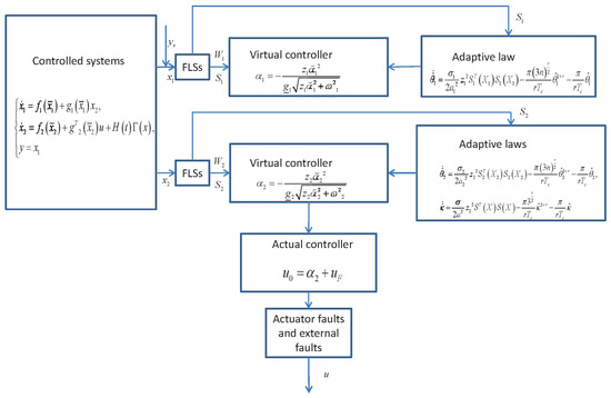
The block diagram of a predefined-time adaptive fuzzy controller is shown in Figure 2.

Figure 2. The block diagram of predefined time adaptive fuzzy controller for Example 1.

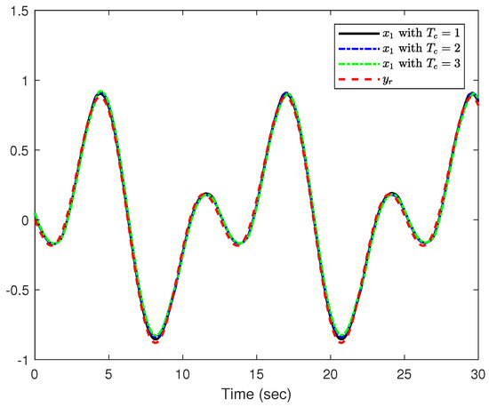
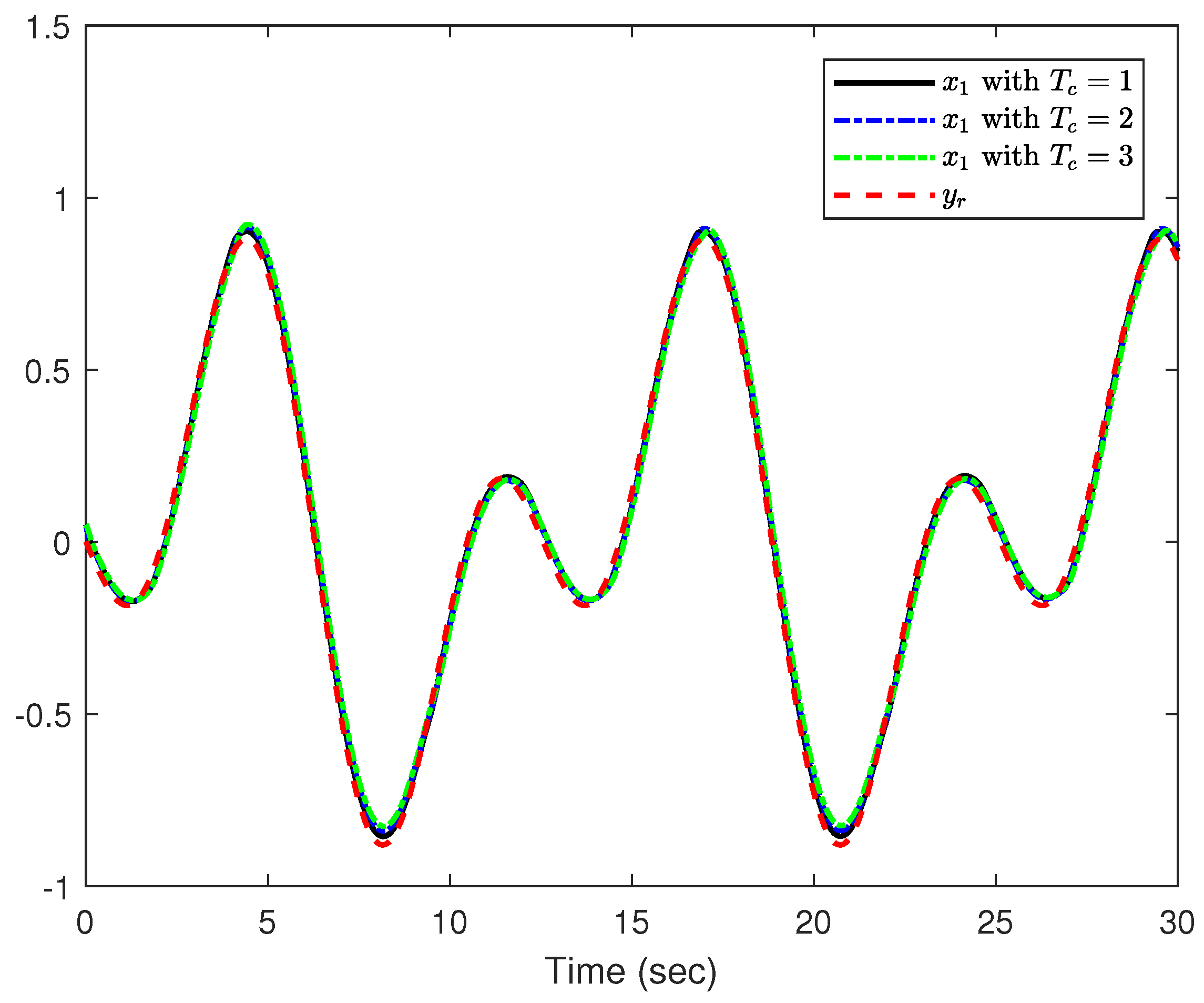
The initial conditions and parameters of the controlled system (83) are presented in Table 1. Three sets of predefined time are set to $2T_c=2$, $2T_c=4$ and $2T_c=6$. The reference signal is selected as $y_r=0.5(\sin \left(0.5t\right)-\sin \left(t\right))$. The actuator faults are set to $u_1=0.6v_1$ and $u_2={\overline{u}}_2=10$ for $t\ge 7s$, and the external fault occurs at $T_{fault}=15s$.

Table 1. Parameters of simulation Example 1.

Parameters	Value	Parameters	Value
$x_1\left(0\right)$	0.05	$x_2\left(0\right)$	0.02
n	2	p	0.1
$g_{2_1}$	1	$g_{2_1}$	1
r	0.35	${\underline{g}}_1$	1
${\overline{g}}_1$	3	${\omega }_1$	0.3
${\omega }_2$	0.3	$a_1$	5
$a_2$	5	a	5
${\sigma }_1$	5	${\sigma }_2$	1.5
$\sigma$	1.5	$\lambda$	0.1

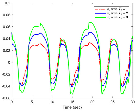
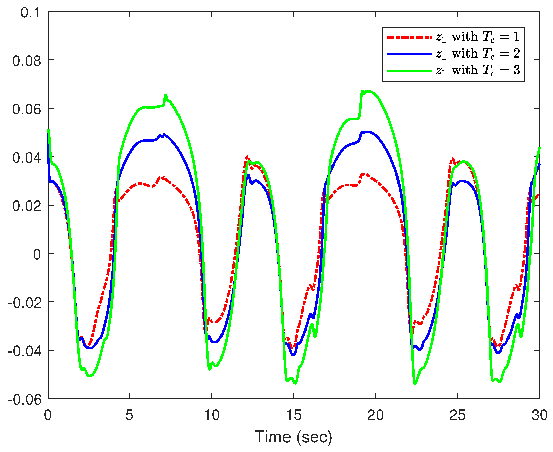
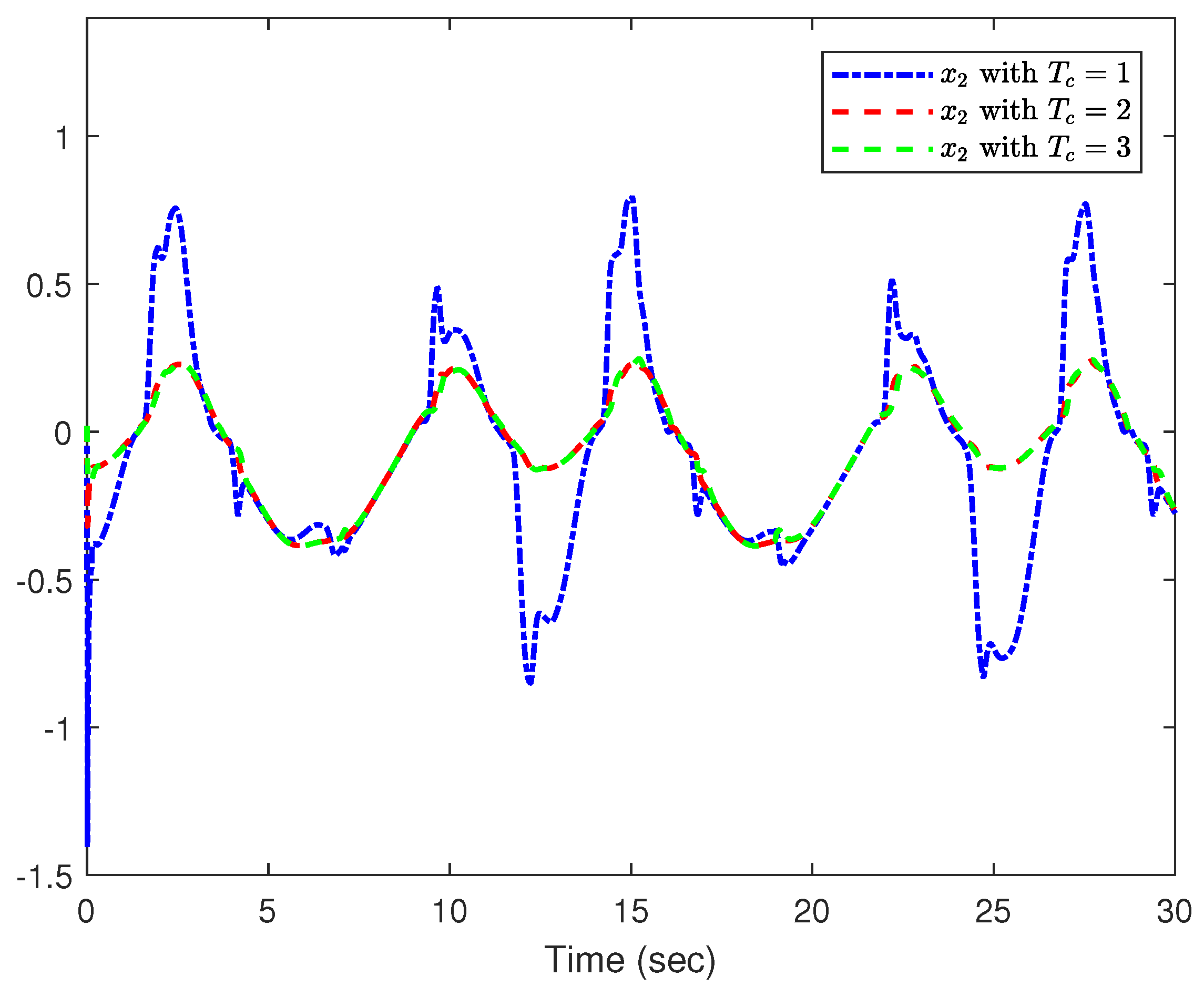
The simulation results are presented in Figure 3, Figure 4, Figure 5, Figure 6 and Figure 7. Figure 3 represents the system output y and the tracking signal $y_r$. Figure 4 shows the trajectory of the tracking error $z_1$. Figure 5 displays the trajectory of the system state $x_2$. Figure 6 displays the trajectories of the actual control inputs $u_1$ and $u_2$. Figure 7 is the curves of adaptive parameters ${\widehat{\theta }}_1$, ${\widehat{\theta }}_2$ and $\widehat{\kappa }$. Based on the simulation results, we can draw the conclusion that all the closed-loop system signals remain bounded and the tracking error can converge to a predefined accuracy within the predefined time.

Figure 3. System output y and reference signal $y_r$ of Example 1.

Figure 4. Tracking error $z_1$ of Example 1.

Figure 5. State variable $x_2$ of Example 1.

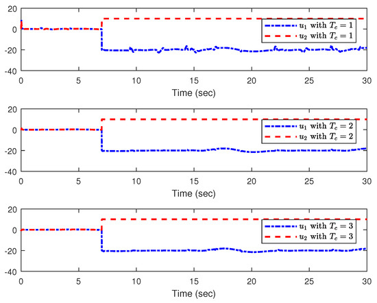
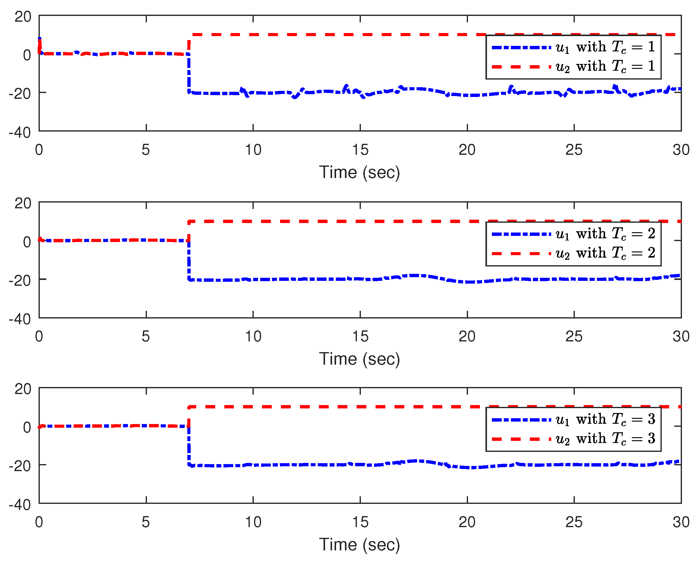
Figure 6. The actual control inputs $u_1$ and $u_2$ of Example 1.

Figure 7. Adaptive laws ${\widehat{\theta }}_1$, ${\widehat{\theta }}_2$ and $\widehat{\kappa }$.

Example 2. 

For the one-link manipulator with multiple faults:

$$\begin{array}{c}\hfill \left\{\begin{array}{c}D\ddot{q}+B\dot{q}+N\sin \left(q\right)=\tau \hfill \\ M\dot{\tau }+H\tau =g^{T}u+H\left(t\right)\Gamma \left(x\right)-K_m\dot{q},\hfill \end{array}\right.\end{array}$$

(89)

where q stands for the link position, $\dot{q}$ expresses the velocity, and $\ddot{q}$ is the acceleration; τ is the torque produced by the motor and $u=[u_1,u_2]$ is the control input with multiple faults. The parameters are selected to $D=B=M=1$, $N=H=10$, $K_m=2$. Then, we make $x_1=q$, $x_2=\dot{q}={\dot{x}}_1$ and $x_3=\tau$, and the system (89) can be rewritten as

$$\begin{array}{c}\hfill \left\{\begin{array}{c}{\dot{x}}_1=f_1\left({\overline{x}}_1\right)+g_1\left({\overline{x}}_1\right)x_2\hfill \\ {\dot{x}}_2=f_2\left({\overline{x}}_2\right)+g_2\left({\overline{x}}_2\right)x_3\hfill \\ {\dot{x}}_3=f_3\left({\overline{x}}_3\right)+g^{T}u+H\left(t\right)\Gamma \left(x\right)\hfill \\ y=x_1\hfill \end{array}\right.\end{array}$$

(90)

where $g_1\left({\overline{x}}_1\right)=g_2\left({\overline{x}}_2\right)=1$, $g={[1,2]}^T$, $f_1\left({\overline{x}}_1\right)=0$, $f_2\left({\overline{x}}_2\right)=-x_2-10\sin \left(x_1\right)+x_1^{2}cos\left(x_2\right)$, $f_3\left({\overline{x}}_3\right)=-2x_2-10x_3$.

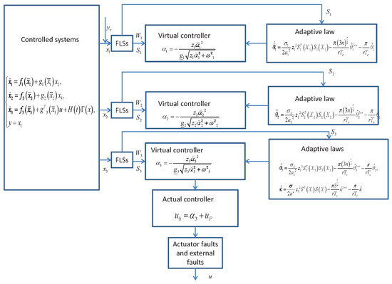
The block diagram of predefined-time adaptive fuzzy controller is diplayed in Figure 8.

Figure 8. The block diagram of predefined time adaptive fuzzy controller for Example 2.

The initial values and adjustable parameters of (90) are represented in Table 2. The predefined times are set to $2T_c=4$ and $2T_c=6$. The reference signal is $y_r=0.5(\sin \left(0.5t\right)-\sin \left(t\right))$. The actuator faults are set to $u_1=0.6v_1$ and $u_2={\overline{u}}_2=15$ for $t\ge 5s$, and the external fault occurs at $T_{fault}=10s$.

Table 2. Parameters of simulation Example 2.

Parameters	Value	Parameters	Value
$x_1\left(0\right)$	0.01	$x_2\left(0\right)$	0.02
$x_3\left(0\right)$	0.01	n	3
p	10	$g_{3_1}$	1
$g_{3_2}$	2	r	0.1
${\underline{g}}_1$	1	${\overline{g}}_1$	1
${\omega }_1$	0.1	${\omega }_2$	0.1
$a_1$	1	$a_2$	1
$a_3$	1	a	1.5
${\sigma }_1$	5	${\sigma }_2$	10
${\sigma }_3$	10	$\sigma$	10
$\lambda$	0.15

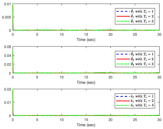
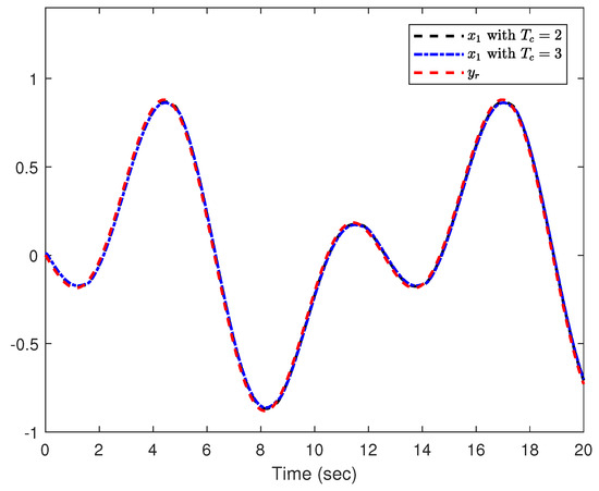
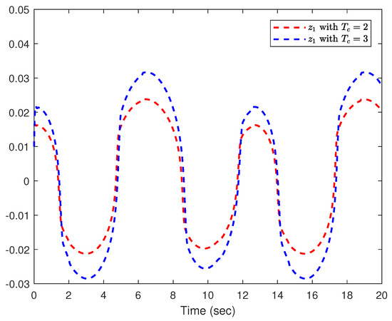
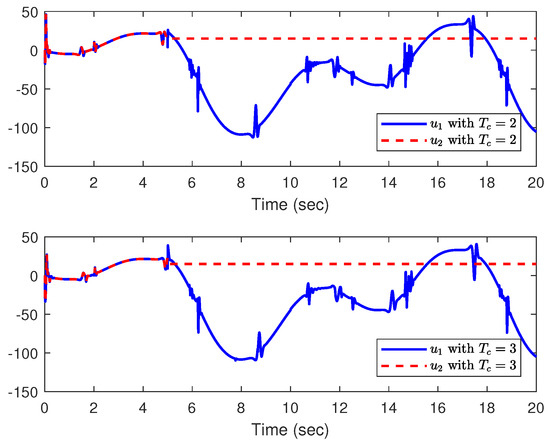
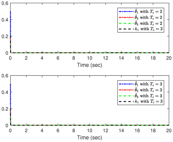
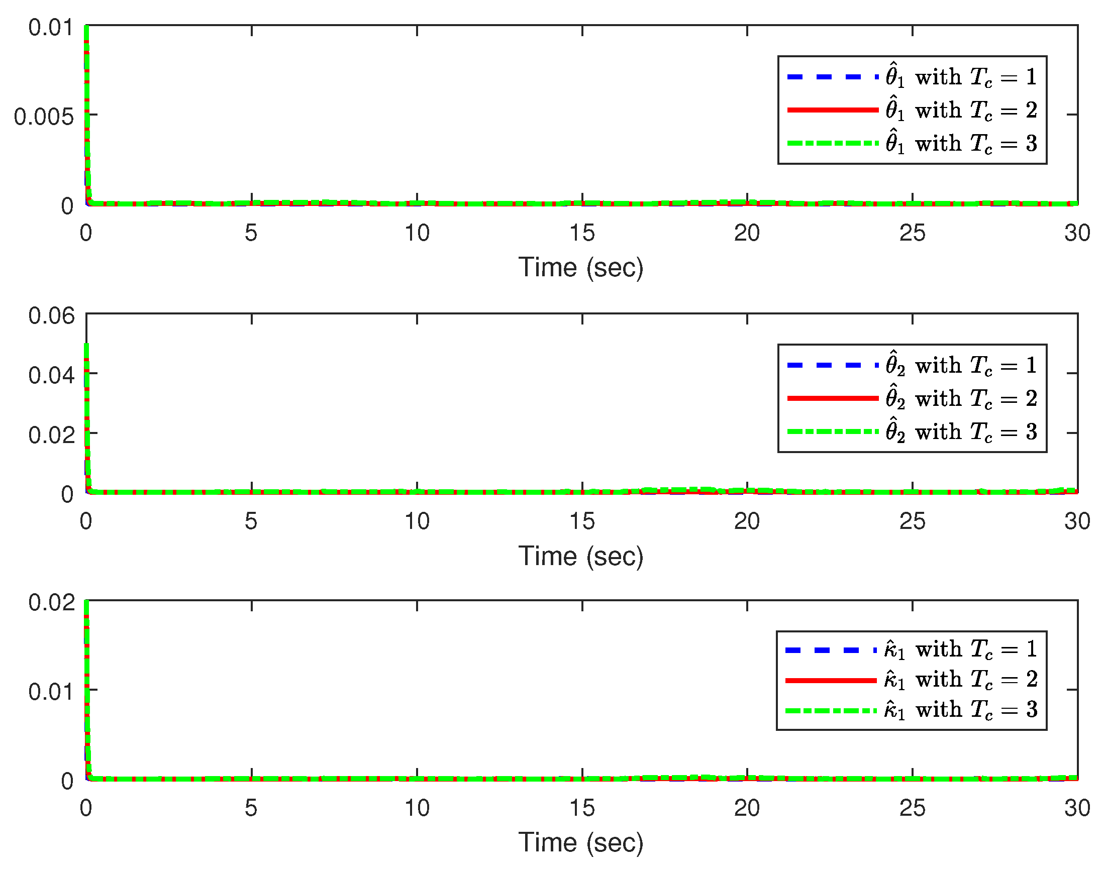
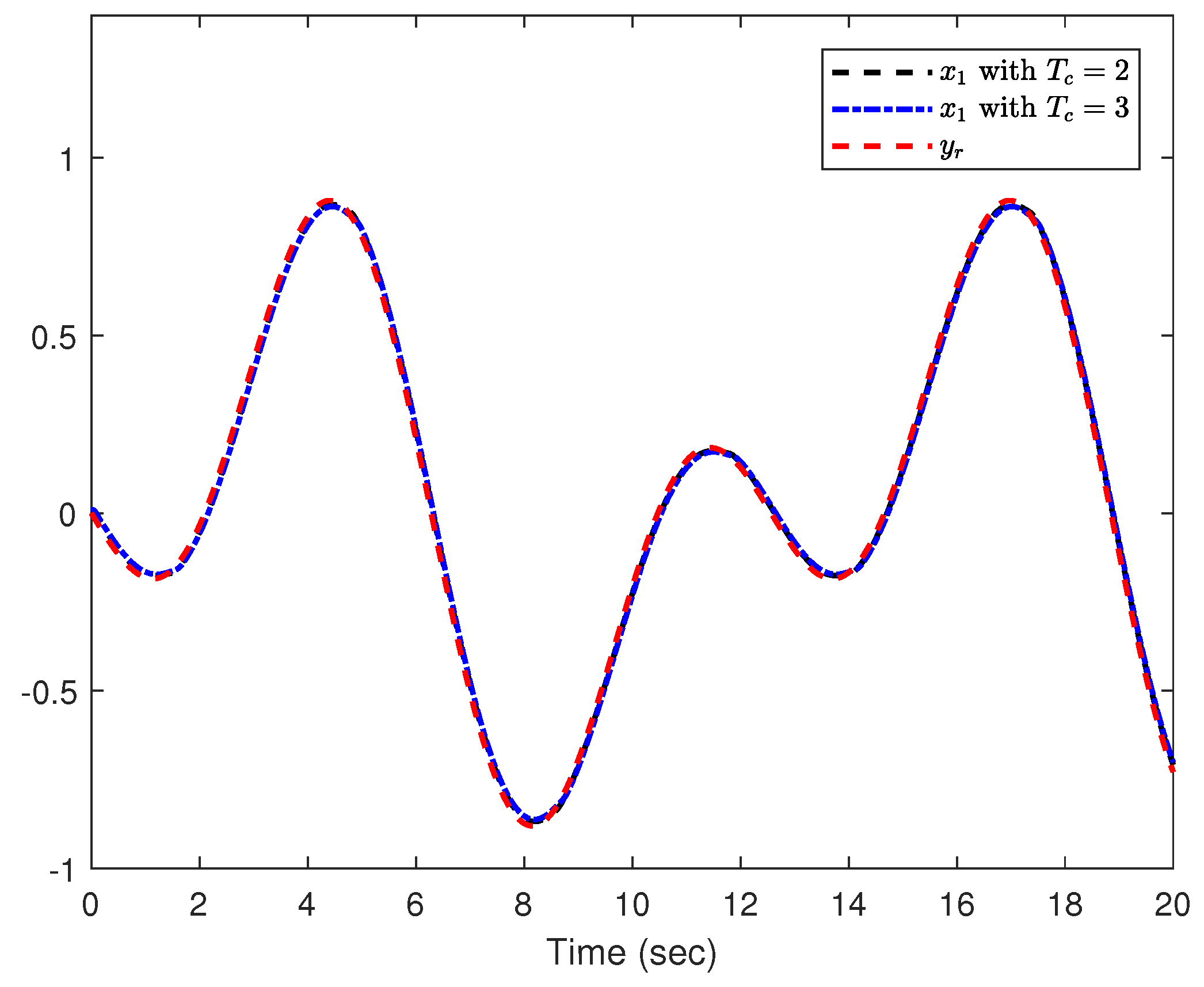
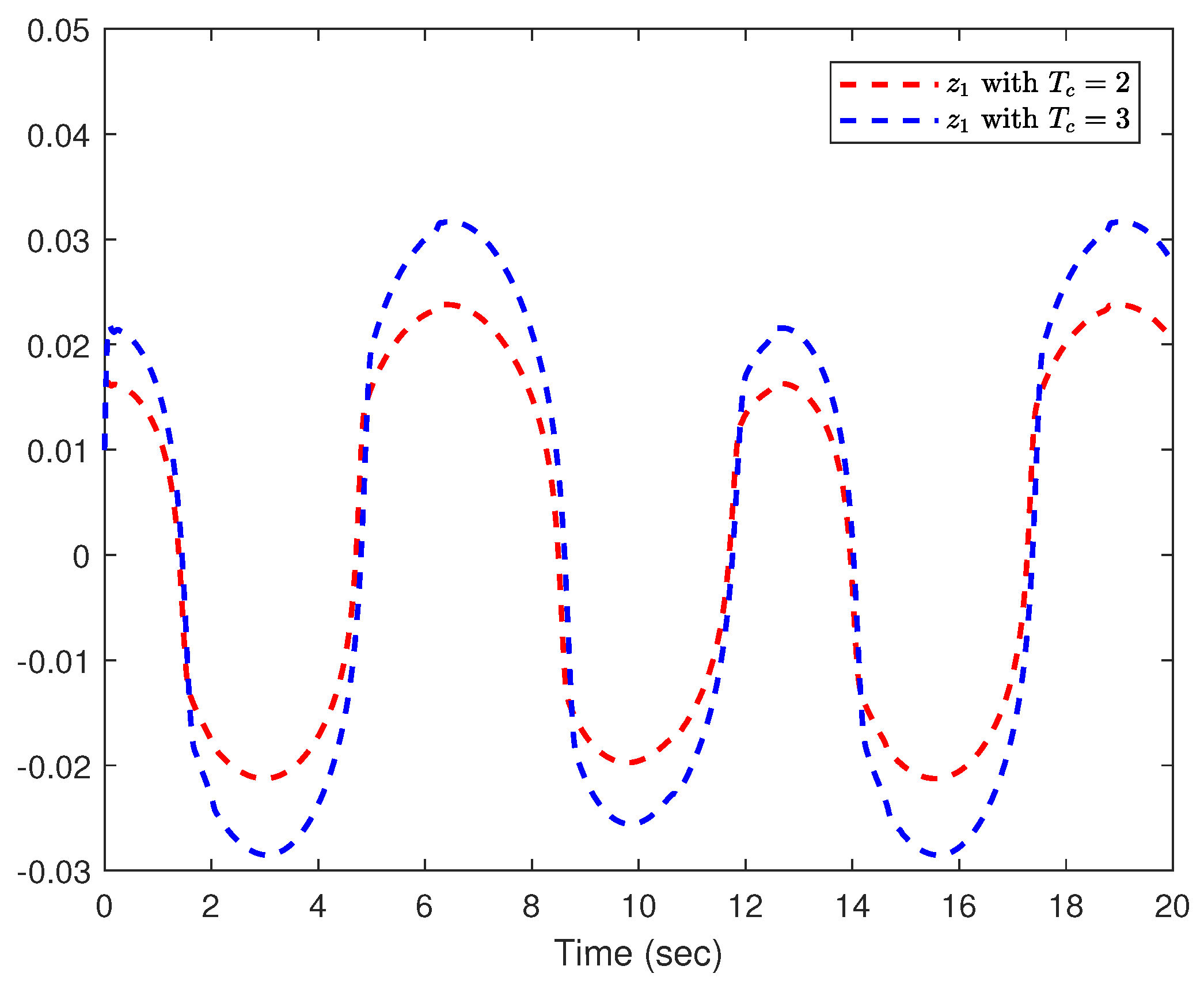
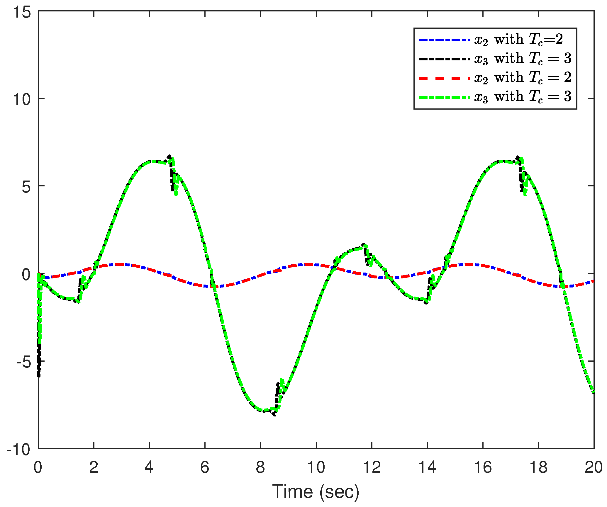
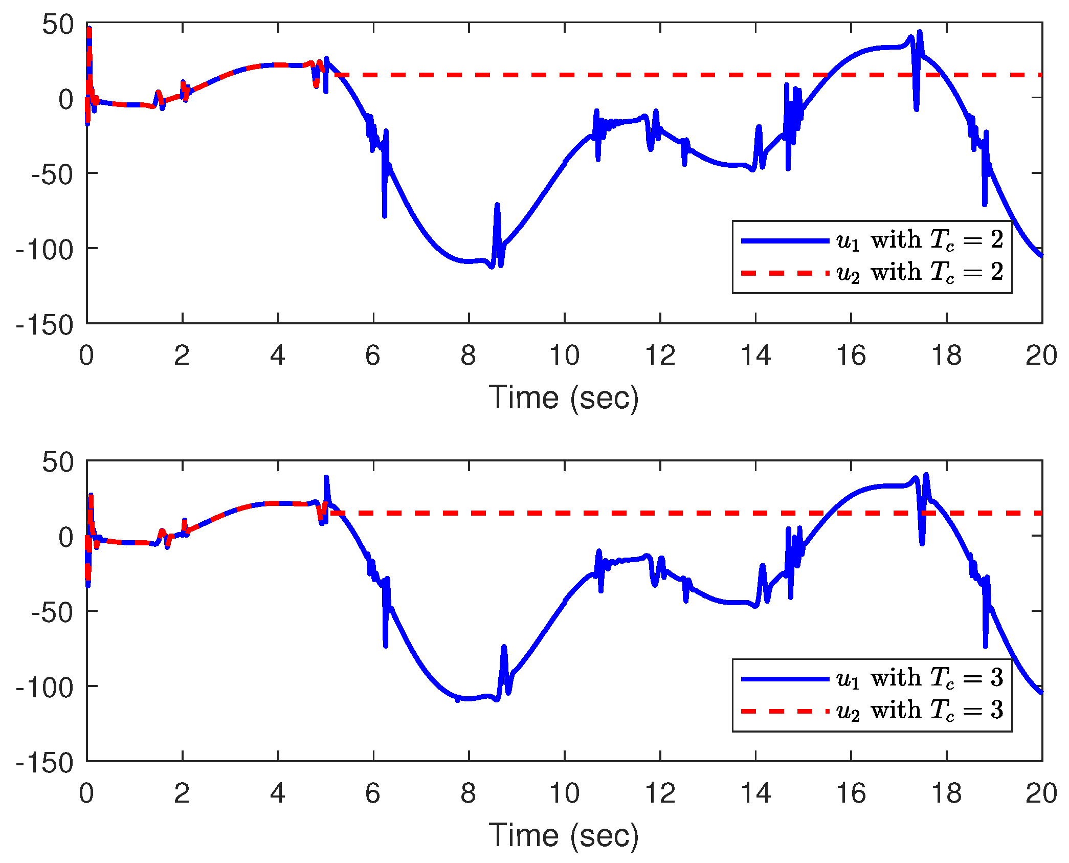
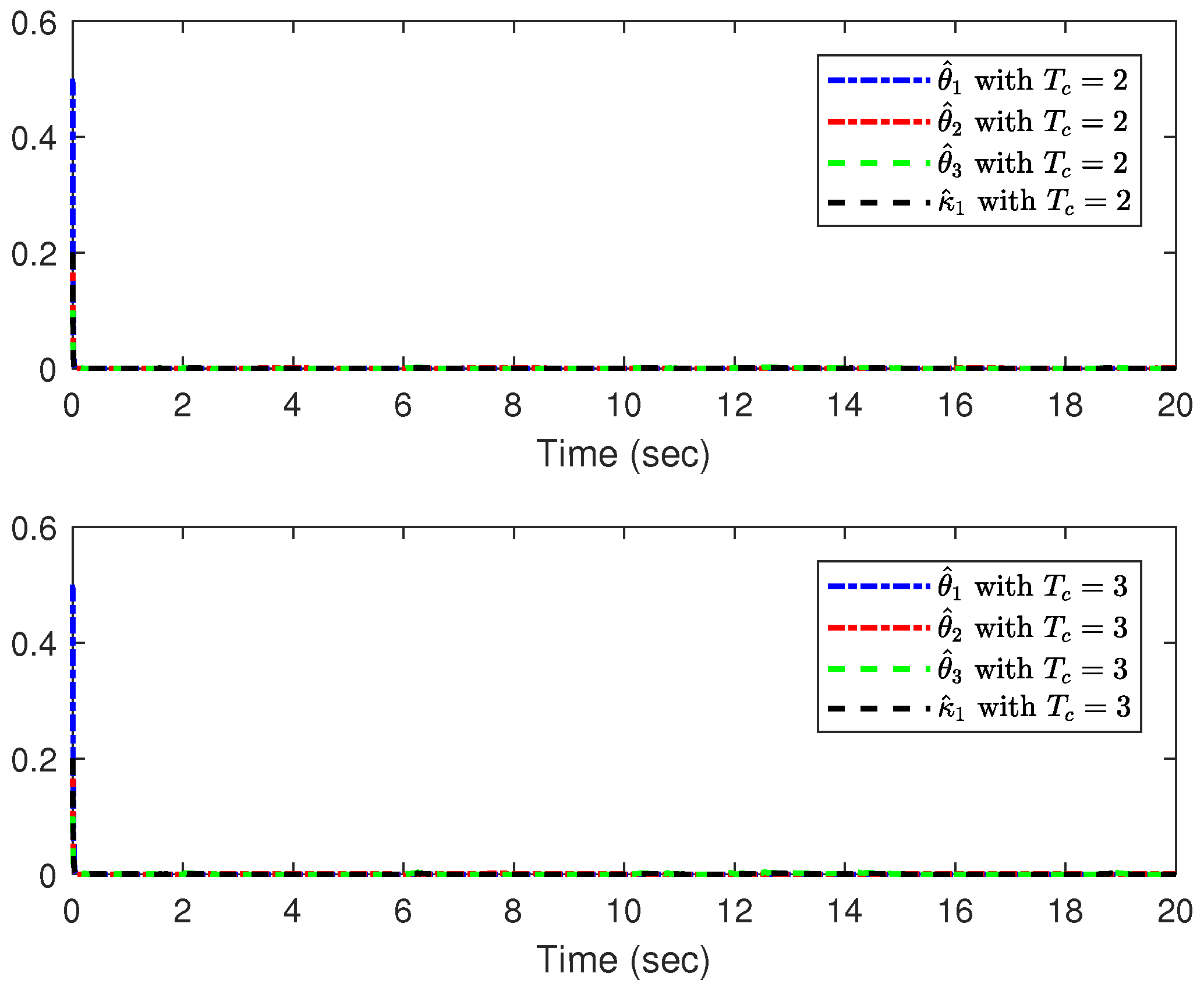
The simulation results are shown in Figure 9, Figure 10, Figure 11, Figure 12 and Figure 13, in which the system output y and tracking signal $y_r$ are represented in Figure 9, Figure 10 displays the tracking error $z_1$, Figure 11 is the trajectory of the system states $x_2$ and $x_3$, actual control inputs $u_1$ and $u_2$ are displayed in Figure 12, and Figure 13 expresses the curves of adaptive parameters ${\widehat{\theta }}_1$, ${\widehat{\theta }}_2$, ${\widehat{\theta }}_3$ and $\widehat{\kappa }$. According to the results, we can conclude that all the closed-loop system signals meet the predefined time-bound conditions and the tracking error can converge to a predefined neighborhood.

Figure 9. System output y and reference signal $y_r$ of Example 2.

Figure 10. Tracking error $z_1$ of Example 2.

Figure 11. State variable $x_2$ of Example 2.

Figure 12. The actual control inputs $u_1$ and $u_2$ of Example 2.

Figure 13. Adaptive laws ${\widehat{\theta }}_1$, ${\widehat{\theta }}_2$ and $\widehat{\kappa }$ of Example 2.

Therefore, Examples 1 and 2 demonstrate the effectiveness of the control strategy presented in this paper.

5. Conclusions

In this research, the predefined time and accuracy adaptive fault-tolerant control problem has been investigated for a class of strict-feedback nonlinear systems with multiple faults. FLSs were employed to model the unknown parts of the systems. Based on the predefined time theory, a condition has been proposed that enables the tracking error to converge to the expected accuracy within predefined time while avoiding singularity issues. Combined with the backstepping mechanism, an adaptive fault-tolerant control strategy has been presented. The controller can ensure that all signals in the closed-loop system are bounded, and the tracking error meets the requirements of predefined accuracy and time. The results of two numerical simulation examples proved the effectiveness of the presented control strategy.

In addition, in future learning and research, we will extend the control strategy proposed in this article to fractional-order systems.

References

- Ma, J.; Zheng, Z.; Li, P. Adaptive dynamic surface control of a class of nonlinear systems with unknown direction control gains and input saturation. IEEE Trans. Cybern. 2015, 45, 728–741. [Google Scholar] [CrossRef]
- Zhou, J.; Wen, C.; Wang, W.; Yang, F. Adaptive backstepping control of nonlinear uncertain systems with quantized states. IEEE Trans. Autom. Control 2019, 64, 4756–4763. [Google Scholar] [CrossRef]
- Tang, G.; Dong, R.; Gao, H. Optimal sliding mode control for nonlinear systems with time-delay. Nonlinear Anal. Hybrid Syst. 2008, 2, 891–899. [Google Scholar] [CrossRef]
- Xu, N.; Zhao, X.; Zong, G.; Wang, Y. Adaptive control design for uncertain switched nonstrict-feedback nonlinear systems to achieve asymptotic tracking performance. Appl. Math. Comput. 2021, 408, 126344. [Google Scholar] [CrossRef]
- Wang, C.; Wen, C.; Hu, Q. Event-triggered adaptive control for a class of nonlinear systems with unknown control direction and sensor faults. IEEE Trans. Autom. Control 2020, 65, 763–770. [Google Scholar] [CrossRef]
- Jiang, D.; Jiang, W.; Zhu, X.; Yin, X. Adaptive control for full-states constrained nonlinear systems with unknown control direction using barrier Lyapunov functionals. Trans. Inst. Meas. Control 2022, 44, 2967–2977. [Google Scholar] [CrossRef]
- Chen, B.; Lin, C.; Liu, X.; Liu, K. Adaptive fuzzy tracking control for a class of MIMO nonlinear systems in nonstrict-feedback form. IEEE Trans. Cybern. 2015, 45, 2744–2755. [Google Scholar] [CrossRef]
- Ma, J.; Xu, S.; Zhuang, G.; Wei, Y.; Zhang, Z. Adaptive neural network tracking control for uncertain nonlinear systems with input delay and saturation. Int. J. Robust Nonlinear Control 2020, 30, 2593–2610. [Google Scholar] [CrossRef]
- Sun, W.; Su, S.; Wu, Y. Novel adaptive fuzzy control for output constrained stochastic nonstrict feedback nonlinear systems. IEEE Trans. Fuzzy Syst. 2020, 29, 1188–1197. [Google Scholar] [CrossRef]
- He, Y.; Chang, X.; Wang, H. Command-filtered adaptive fuzzy control for switched MIMO nonlinear systems with unknown dead zones and full state constraints. Int. J. Fuzzy Syst. 2023, 25, 544–560. [Google Scholar] [CrossRef]
- Yu, T.; Liu, Y.; Liu, L. Adaptive fuzzy control of nonlinear systems with function constraints based on time-varying IBLFs. IEEE Trans. Fuzzy Syst. 2022, 30, 4939–4952. [Google Scholar] [CrossRef]
- Li, M.; Xiang, Z. Adaptive neural network tracking control for a class of switched nonlinear systems with input delay. Neurocomputing 2019, 366, 284–294. [Google Scholar] [CrossRef]
- Yang, D.; Zong, G.; Liu, Y.; Choon, K. Adaptive neural network output tracking control of uncertain switched nonlinear systems: An improved multiple Lyapunov function method. Inf. Sci. 2022, 606, 380–396. [Google Scholar] [CrossRef]
- Wang, H.; Chen, B.; Lin, C.; Sun, Y. Observer-based adaptive neural control for a class of nonlinear pure-feedback systems. Neurocomputing 2016, 171, 1517–1523. [Google Scholar] [CrossRef]
- Liu, J.; Jiang, Y. Adaptive fuzzy control for high-order nonlinear systems with time-varying full-state constraints and input saturation. Int. J. Adapt. Control Signal Process. 2023, 37, 710–725. [Google Scholar] [CrossRef]
- Zhang, J.; Yang, G. Robust adaptive fault-tolerant control for a class of unknown nonlinear systems. IEEE Trans. Ind. Electron. 2017, 64, 585–594. [Google Scholar] [CrossRef]
- Zhang, H.; Cui, Y.; Wang, Y. Hybrid fuzzy adaptive fault-tolerant control for a class of uncertain nonlinear systems with unmeasured states. IEEE Trans. Fuzzy Sys. 2017, 25, 1041–1050. [Google Scholar] [CrossRef]
- Wang, J.; Pan, H.; Sun, W. Event-triggered adaptive fault-tolerant control for unknown nonlinear systems with applications to linear motor. IEEE/ASME Trans. Mech. 2022, 27, 940–949. [Google Scholar] [CrossRef]
- Zhang, S.; Huang, C.; Ji, K. Prescribed performance incremental adaptive optimal fault-tolerant control for nonlinear systems with actuator faults. ISA Trans. 2022, 120, 99–109. [Google Scholar] [CrossRef]
- Li, Y.; Yang, G. Adaptive asymptotic tracking control of uncertain nonlinear systems with input quantization and actuator faults. Automatica 2016, 72, 177–185. [Google Scholar] [CrossRef]
- Wang, Y.; Xu, N.; Liu, Y. Adaptive fault-tolerant control for switched nonlinear systems based on command filter technique. Appl. Math. Comput. 2021, 392, 125725. [Google Scholar] [CrossRef]
- Zhang, Z.; Wen, C.; Xing, L.; Song, Y. Event-triggered adaptive control for a class of nonlinear systems with mismatched uncertainties via intermittent and faulty output feedback. IEEE Trans. Autom. Control 2023, 68, 8142–8149. [Google Scholar] [CrossRef]
- Jia, F.; He, X. Adaptive fault-tolerant tracking control for discrete-time nonstrict-feedback nonlinear systems with stochastic noises. IEEE Trans. Autom. Sci. Eng. 2023, 1–13. [Google Scholar] [CrossRef]
- Zeng, X.; Shen, Q. Adaptive fault-tolerant control for high-order nonlinear systems with supervisory controllers and command filters. Int. J. Control Autom. Syst. 2023, 21, 12–19. [Google Scholar] [CrossRef]
- Yin, S.; Gao, H.; Qiu, J.; Kaynak, O. Adaptive fault-tolerant control for nonlinear system with unknown control directions based on fuzzy approximation. IEEE Trans. Syst. Man Cybern. Syst. 2017, 47, 1909–1918. [Google Scholar] [CrossRef]
- Qi, H.; Chen, M.; Wu, L. Adaptive fault-tolerant control of nonlinear systems based on tuning functions. Int. J. Robust Nonlinear Control 2023, 33, 6715–6733. [Google Scholar] [CrossRef]
- Milecki, A.; Nowak., P. Review of fault-tolerant control systems used in robotic manipulators. Appl. Sci. 2023, 13, 2675. [Google Scholar] [CrossRef]
- Ali, K.; Mehmood., A.; Iqbal., J. Fault-tolerant scheme for robotic manipulator-Nonlinear robust back-stepping control with friction compensation. PLoS ONE 2021, 16, e0256491. [Google Scholar] [CrossRef]
- Zhai, D.; An, L.; Li, X.; Zhang, Q. Adaptive fault-tolerant control for nonlinear systems with multiple sensor faults and unknown control directions. IEEE Trans. Neural Netw. Learn. Syst. 2018, 29, 4436–4446. [Google Scholar] [CrossRef]
- Lin, W.; Lin, C.; Sun, Z. Adaptive multiple fault detection and alarm processing for loop system with probabilistic network. IEEE Trans. Power Deliv. 2004, 19, 64–69. [Google Scholar] [CrossRef]
- Jiang, X.; Mu, X.; Hu, Z. Decentralized adaptive fuzzy tracking control for a class of nonlinear uncertain interconnected systems with multiple faults and denial-of-service attack. IEEE Trans. Fuzzy Syst. 2021, 29, 3130–3141. [Google Scholar] [CrossRef]
- Lin, Y.; Lu, F.; Cheng, K. Multiple-fault diagnosis based on adaptive diagnostic test pattern generation. IEEE Trans. Comput.-Aided Des. Integr. Circuits Syst. 2007, 26, 932–942. [Google Scholar] [CrossRef]
- Li, N.; Han, Y.; He, W.; Zhu, S. A novel network-based controller design for a class of stochastic nonlinear systems with multiple faults and full state constraints. Int. J. Control 2023, 97, 651–661. [Google Scholar] [CrossRef]
- Sun, Y.; Chen, B.; Lin, C.; Wang, H. Finite-time adaptive control for a class of nonlinear systems with nonstrict feedback structure. IEEE Trans. Cybern. 2018, 48, 2774–2782. [Google Scholar] [CrossRef] [PubMed]
- Sui, S.; Chen, L.; Tong, S. Neural network filtering control design for nontriangular structure switched nonlinear systems in finite time. IEEE Trans. Neural Netw. Learn. Syst. 2019, 30, 2153–2162. [Google Scholar] [CrossRef] [PubMed]
- Sui, S.; Chen, L.; Tong, S. Finite-time adaptive fuzzy prescribed performance control for high-order stochastic nonlinear systems. IEEE Trans. Fuzzy Syst. 2021, 30, 2227–2240. [Google Scholar] [CrossRef]
- Wu, Y.; Pan, Y.; Chen, M.; Li, H. Quantized adaptive finite-time bipartite NN tracking control for stochastic multiagent systems. IEEE Trans. Cybern. 2021, 51, 2870–2881. [Google Scholar] [CrossRef] [PubMed]
- Sui, S.; Chen, L.; Tong, S. Fuzzy adaptive finite-time control design for nontriangular stochastic nonlinear systems. IEEE Trans. Fuzzy Syst. 2019, 27, 172–184. [Google Scholar] [CrossRef]
- Wang, H.; Bai, W.; Liu, X. Finite-time adaptive fault-tolerant control for nonlinear systems with multiple faults. IEEE/CAA J. Autom. Sin. 2019, 6, 1417–1427. [Google Scholar] [CrossRef]
- Polyakov, A. Nonlinear feedback design for fixed-time stabilization of linear control systems. IEEE Trans. Autom. Control 2011, 57, 2106–2110. [Google Scholar] [CrossRef]
- Sun, Y.; Zhang, L. Fixed-time adaptive fuzzy control for uncertain strict feedback switched systems. Inf. Sci. 2021, 546, 742–752. [Google Scholar] [CrossRef]
- Mei, Y.; Li, F.; Xia, R.; Park, J.; Shen, H. Fixed-time adaptive neural tracking control for nonstrict-feedback nonlinear systems with mismatched disturbances using an event-triggered scheme. Nonlinear Dyn. 2023, 111, 5383–5400. [Google Scholar] [CrossRef]
- Lu, K.; Liu, Z.; Wang, Y.; Chen, L. Fixed-time adaptive fuzzy control for uncertain nonlinear systems. IEEE Trans. Fuzzy Syst. 2021, 29, 3769–3781. [Google Scholar] [CrossRef]
- Fang, X.; Fan, H.; Liu, L. Adaptive fixed-time fault-tolerant control of saturated MIMO nonlinear systems with time-varying state constrains. Nonlinear Dyn. 2022, 110, 3463–3483. [Google Scholar] [CrossRef]
- Cui, D.; Xiang, Z. Nonsingular fixed-time fault-tolerant fuzzy control for switched uncertain nonlinear systems. IEEE Trans. Fuzzy Syst. 2022, 31, 174–183. [Google Scholar] [CrossRef]
- Zhang, X.; Tan, J.; Wu, J. Event-triggered-based fixed-time adaptive neural fault-tolerant control for stochastic nonlinear systems under actuator and sensor faults. Nonlinear Dyn. 2022, 108, 2279–2296. [Google Scholar] [CrossRef]
- Sanchez-Torres, J.; Sanche, E.; Loukianov, A. Predefined-time stability of dynamical systems with sliding modes. In Proceedings of the 2015 American Control Conference (ACC), Chicago, IL, USA, 1–3 July 2015. [Google Scholar] [CrossRef]
- Wang, H.; Tong, M.; Zhao, X.; Niu, B.; Yang, M. Predefined-time adaptive neural tracking control of switched nonlinear systems. IEEE Trans. Cybern. 2022, 53, 6538–6548. [Google Scholar] [CrossRef] [PubMed]
- Fu, L.; Ma, R.; Pang, H.; Fu, J. Predefined-time tracking of nonlinear strict-feedback systems with time-varying output constraints. J. Frankl. Inst. 2022, 359, 3492–3516. [Google Scholar] [CrossRef]
- Jimenez-Rodriguez, E.; Munoz-Vazquez, A.; Sanchez-Torres, J.; Defoort, M.; Loukianov, A. A Lyapunov-like characterization of predefined-time stability. Trans. Autom. Control 2020, 65, 4922–4927. [Google Scholar] [CrossRef]
- Jia, F.; Huang, J.; He, X. Predefined-time fault-tolerant control for a class of nonlinear systems with actuator faults and unknown mismatched disturbances. IEEE Trans. Autom. Sci. Eng. 2023, 1–15. [Google Scholar] [CrossRef]
- Wang, Q.; Cao, J.; Liu, H. Adaptive fuzzy fontrol of nonlinear systems with predefined time and accuracy. IEEE Trans. Fuzzy Syst. 2022, 30, 5152–5165. [Google Scholar] [CrossRef]
- Ni, J.; Shi, P. Global predefined time and accuracy adaptive neural network control for uncertain strict-feedback systems with output constraint and dead zone. IEEE Trans. Syst. Man Cybern. Syst. 2021, 51, 7903–7918. [Google Scholar] [CrossRef]
- Li, P.; Yang, G. Backstepping adaptive fuzzy control of uncertain nonlinear systems against actuator faults. J. Control Theory Appl. 2009, 7, 248–256. [Google Scholar] [CrossRef]
- Tang, X.; Tao, G.; Joshi, S. Adaptive actuator failure compensation for nonlinear MIMO systems with an aircraft control application. Automatica 2007, 43, 1869–1883. [Google Scholar] [CrossRef]
- Fekih, A. Fault-tolerant flight control design for effective and reliable aircraft systems. J. Control Decis. 2014, 1, 299–316. [Google Scholar] [CrossRef]
- Li, Y.; He, J.; Zhang, Q.; Zhang, W.; Li, Y. Predefined-time fault-tolerant trajectory tracking control for autonomous underwater vehicles considering actuator saturation. Actuators 2023, 12, 171. [Google Scholar] [CrossRef]
- Jimenez-Rodriguez, E.; Snchez-Torres, J.; Loukianov, A. On optimal predefined-time stabilization. Int. J. Robust Nonlinear 2017, 27, 3620–3642. [Google Scholar] [CrossRef]
- Jimenez-Rodriguez, E.; Munoz-Vazquez, A.; Sanchez-Torres, J.; Alexander, G. Loukianov: A note on predefined-time stability. IFAC-PapersOnLine 2018, 51, 520–525. [Google Scholar] [CrossRef]
- Jimenez-Rodriguez, E.; Sanchez-Torres, J.; Gomez-Gutierrez, D.; Alexander, G. Loukinanov. Variable structure predefined-time stabilization of second-order systems. Asian J. Control 2019, 21, 1179–1188. [Google Scholar] [CrossRef]
- Wang, L. Adaptive Fuzzy Systems and Control: Design and Stability Analysis; Prentice-Hall: Englewood Cliffs, NJ, USA, 1994. [Google Scholar]
- Gang, T.; Kokotovic, P. Adaptive control of plants with unknown dead-zones. IEEE Trans. Autom. Control 1994, 39, 59–68. [Google Scholar] [CrossRef]
- Cao, J.; Li, R. Fixed-time synchronization of delayed memristor-based recurrent neural networks. Sci. China Inform. Sci. 2017, 60, 032201. [Google Scholar] [CrossRef]
- Wang, C.; Lin, Y. Decentralized adaptive tracking control for a class of interconnected nonlinear time-varying systems. Automatica 2015, 54, 16–24. [Google Scholar] [CrossRef]
- Qian, C.; Lin, W. Non-Lipschitz continuous stabilizers for nonlinear systems with uncontrollable unstable linearization. Syst. Control Lett. 2001, 42, 185–200. [Google Scholar] [CrossRef]
- Sun, Y.; Wang, F.; Liu, Z.; Zhang, Y.; Chen, C. Fixed-time fuzzy control for a class of nonlinear systems. IEEE Trans. Cybern. 2020, 52, 3880–3887. [Google Scholar] [CrossRef]
Disclaimer/Publisher’s Note: The statements, opinions and data contained in all publications are solely those of the individual author(s) and contributor(s) and not of MDPI and/or the editor(s). MDPI and/or the editor(s) disclaim responsibility for any injury to people or property resulting from any ideas, methods, instructions or products referred to in the content. |
© 2024 by the authors. Licensee MDPI, Basel, Switzerland. This article is an open access article distributed under the terms and conditions of the Creative Commons Attribution (CC BY) license (https://creativecommons.org/licenses/by/4.0/).