Progressive Optimal Fault-Tolerant Control Combining Active and Passive Control Manners

Abstract

This study develops a progressive optimal fault-tolerant control method based on insufficient fault information. By combining passive and active fault-tolerant control manners during the process of fault diagnosis, insufficient fault information is fully used, and optimal fault-tolerant control effect is achieved. In addition, the fault-tolerant control method based on guaranteed robust cost control is introduced. The proposed progressive optimal fault-tolerant control method considers two aspects. First, as the amount of fault information continually increases, the performance index of the progressive optimal fault-tolerant controller improves. Second, at each moment, based on the corresponding insufficient fault information and prior knowledge, optimal fault-tolerant control is achieved according to current fault information. The process of progressive optimal fault-tolerant control converges to active fault-tolerant control when the fault is completely identified, and the optimal fault-tolerant controller is no longer reconfigured until no more useful fault information can be provided. Furthermore, a progressive optimal fault-tolerant control algorithm based on the grid segmentation in the parameter uncertainty domain and the selection of different auxiliary center points is introduced. Simulation results verified the feasibility of the proposed algorithm and the validity of the proposed theory.

1. Introduction

In industrial systems, fault diagnosis (FD) and fault-tolerant control (FTC) are closely related. In recent years, there have been many studies on fault diagnosis and fault-tolerant control in various fields, including aerospace [1,2,3] and fields associated with power systems [4,5,6], high-speed rail systems [7,8,9,10,11], and satellites [12,13]. Based on previous research, fault diagnosis will inevitably develop in a faster and more accurate way in the future. Obtaining fast and accurate fault information is an essential requirement of active fault-tolerant control (AFTC) to ensure safe system operation; otherwise, AFTC performance cannot be guaranteed, and its implementation cannot even be guaranteed. As is well known, passive fault-tolerant control (PFTC) is relatively conservative. However, unlike AFTC, PFTC does not require real-time fault information, which represents its inherent advantage. Traditional fault diagnosis is predominantly based on mathematical models [14,15,16]; however, model-based methods for fault diagnosis require an accurate system model, and the majority of these methods can only provide only two types of results (i.e., fault undiagnosed or fault diagnosed). Unfortunately, such approaches do not provide continuous fault information which is insufficient but crucial for effective fault-tolerant control. In recent years, there have been many studies on non-model-based methods (e.g., data-driven methods for fault diagnosis), especially artificial intelligence-based algorithms [17,18,19]. Fault diagnosis using artificial intelligence-based algorithms which include neural networks have a common problem: the behavior inside the “black box” is difficult to determine [20]. Thus, both model-based and non-model-based fault diagnosis methods have their own advantages and disadvantages. However, the development of a more accurate and faster fault diagnosis method remains a challenge.

When fault information cannot be rapidly and accurately obtained, a fault-tolerant control strategy which performs PFTC before the fault is fully identified and then switches to the AFTC after the fault has been completely diagnosed seems to be a good choice. This idea was proposed in [21]. However, its main disadvantage is the failure to utilize incomplete fault information, which is still valuable. Mechanically combining two fault-tolerant control methods is not ideal due to their respective shortcomings [22,23,24]. Therefore, a perfect solution could be generated if the advantages of AFTC and PFTC were to be combined under the condition of insufficient fault information. Existing research has indicated that PFTC and AFTC are typically applied independently, with fewer studies exploring the combination of these two methods. Although hybrid fault-tolerant control [25] combines AFTC and PFTC to a certain extent, these two control types are used separately depending on whether a fault has been fully diagnosed. In [26], a fault-tolerant control system (FTCS) design based on imprecise fault identification and robust reconfigurable control is proposed. This method reduces the time delay between the onset of a fault and the controller reconfiguration so that the system’s stability after the fault occurrence can be recovered rapidly. However, this method mainly emphasizes system stability rather than performance optimization. Moreover, the control object of this method does not have generality. In [27], actuator faults were considered as additive faults, and a combined passive-active FTC method based on reliable control was proposed, achieving a balance between performance and complexity. However, the predefined control laws were obtained offline rather than online by designing bottom-up extensible controllers with a minimal acceptable configuration, and the nominal performance remained at a sub-optimal level after a fault.

Although the above-mentioned methods combining the PFTC and AFTC methods are mostly mechanical, they have been valuable, but insufficient fault information was not fully used in the above-mentioned studies. Moreover, the concept of progressive performance optimization has not been adequately explored, according to which, as fault information increases, the fault-tolerant control effect improves. In view of this, this study examines how to fully use insufficient fault information and combine the PFTC and AFTC methods efficiently to achieve optimal performance. This idea was partly introduced in [28].

A comparison of the existing fault diagnosis methods has indicated that the parameter interval algorithm shows superiority over other algorithms [29]. The parameter interval algorithm can continuously obtain increasingly accurate fault information during the fault diagnosis process. The smaller the parameter interval, the more accurate the fault identification. From the moment of fault occurrence to the moment of complete fault identification, the obtained fault information can be fully used to reconfigure the controller to ensure optimal fault-tolerant control performance.

The pursuit of achieving a robust and optimal control effect while addressing the limitations of practical methods and ensuring system stability, even at the expense of some system performance, has long been a research focus [30,31,32,33]. Robust control methods are often applied to stabilize system uncertainty [34]. Meanwhile, using robust control methods as fault-tolerant control methods to accommodate system faults is another application. Notably, Xue’s study [35] on robust and optimal control, which considers both robustness and the control system’s effectiveness, holds significant value as a reference. Since a system fault can be viewed as system uncertainty, the results of Xue’s research on robust and optimal control can be applied to the field of fault-tolerant control for faulty systems.

The process of a progressive optimal fault-tolerant control method combines the PFTC and AFTC manners, as explained in this article. When a fault occurs, the maximum uncertainty domain can be determined based on prior knowledge. Moreover, the more fault information obtained, the smaller the uncertainty domain of the faulty system. The progressive optimal fault-tolerant control method based on robust guaranteed cost fault-tolerant control has been used to reconfigure the controller and ensure the optimal fault-tolerant control effect with the improving fault information. When a fault is completely identified, the process of progressive optimal fault-tolerant control converges to active fault-tolerant control, and the optimal fault-tolerant controller is no longer reconfigured until no more useful fault information can be provided. The essence of the progressive optimal fault-tolerant control method lies in combining active and passive fault-tolerant control manners by using continuously improving fault information.

The rest of this article is structured as follows: In Section 2, the necessary preliminaries and the problem formulation of progressive optimal fault-tolerant control are provided. Section 3 explores a progressive optimal fault-tolerant control method in a linear uncertain system. A case study is presented in Section 4. Finally, Section 5 concludes this article.

2. Preliminaries and Problem Formulation

A system fault can be considered as a deviation of the system parameters [36]. Therefore, a faulty system can be modeled as an uncertain dynamic system with parameter uncertainty. The area where an actual value point of the system parameter vector might exist is called the uncertainty domain.

An uncertain dynamic system is defined by (1), and its control law is given by (2).

$$\left\{\begin{array}{c}\dot{x}=f(x,\theta ,u)\\ y=\mathbf{C}x\\ \theta ={\theta }_0+\Delta \theta \end{array}\right.$$

(1)

$$u=-Kx$$

(2)

In (1) and (2), $x\in {\mathbf{R}}^n$ represents the system’s state parameter vector, $u\in {\mathbf{R}}^p$ represents the control input, and $y\in \mathbf{R}$ represents the output; $f(•)$ is a non-linear function of $x$ and $u$ parameterized by a vector $\theta$; $C$ represents the output matrix with a proper dimension; $\Delta \theta$ denotes the uncertainty of the parameter vector related to the uncertainty domain $\Omega$, i.e., ${\theta }_0+\Delta \theta \in \Omega$. In this study, it is assumed that the uncertainty domain $\Omega$ surrounds the nominal value ${\theta }_0$ of the system parameter vector $\theta$, and $K\in {\mathbf{R}}^q$ is the controller parameter vector.

The selection of the controller parameter vector $K$ is called controller configuration. It is assumed that this selection is related to the cost function (3).

$$J=F(x,u)$$

(3)

Furthermore, assume that $p_1(x,u),p_2(x,u),\dots p_r(x,u)\dots p_g(x,u)$ are $g$ parameters of a closed-loop system with certain constraint conditions. These $g$ parameters can take eigenvalues of the closed-loop system (1) or other values depending on the application context. The constraint condition of the controller parameter vector $K$ can be defined by (4).

$$p_r(x,u)\in {\Lambda }_r,\forall r=1,2,\dots ,v,\forall K\in \Psi (\Omega ),\forall \theta \in \Omega$$

(4)

The constraint condition (4) implies a set of crucial indexes that should be satisfied and represents the basic constraint condition of the controller parameter selection. In (4), ${\Lambda }_r$ represents a certain domain in a complex plane. For instance, if $p_r$ is an eigenvalue, then ${\Lambda }_r$ can be a left-half s plane. The closed-loop system (1) is considered to have good stability if condition (4) is satisfied.

Definition 1.

All values of controller vector $K$ under constraint condition (4) form a feasible domain $\Psi (\Omega )$ corresponding to an uncertainty domain $\Omega$ [28].

Then, the objective of controller configuration is that the closed-loop system (1) satisfies the following condition:

$$\min J=\min F(x,u)$$

(5)

where $\min J$ can be an analytic or non-analytic expression; for instance, in the general case, it can be a minimizing operation of a quadratic function of system state variables. Alternatively, it could be described non-analytically—“the controller is the simplest to obtain”.

For the state feedback controller (2), (6) is selected as one of the constraint conditions.

$$J\le J^{*}$$

(6)

In (6), $J^{*}$ is a positive number and denotes the upper bound of the performance index $J$.

For the closed-loop system (1) and performance index (3), all controller parameter values $K$ corresponding to the uncertainty domain $\Omega$ that satisfy condition (6) form a feasible domain $\Psi (\Omega )$. Therefore, progressive optimal fault-tolerant control is discussed in the feasible domain $\Psi (\Omega )$ corresponding to the uncertainty domain $\Omega$.

With the narrowing of the uncertainty domain $\Omega$ of a fault, the fault information becomes increasingly sufficient; intuitively, there exists the following relation: $\Omega \supset {\Omega }_1\supset {\Omega }_2\supset \dots \supset {\Omega }_i\supset \dots \supset {\Omega }_j$, where ${\Omega }_i$ denotes the uncertainty domain at the $i\mathrm{th}$ moment. And the $j\mathrm{th}$ moment is after the $i\mathrm{th}$ moment if $j>i$. This indicates that the uncertainty domain $\Omega$ of a fault and its narrowed sub-domains exhibit the nested property.

With the continuous increase in and improvement of fault information, the uncertainty domain of the fault shrinks.

To illustrate the progressive optimal fault-tolerant control method, we first introduce Lemma 1.

Lemma 1.

For an uncertain dynamic system (1), the smaller the range of uncertainty domain $\Omega$ of a fault, the lower the upper bound of the performance index.

Proof. 

Consider an arbitrary sub-domain ${\Omega }_i$ of an uncertainty domain $\Omega$ of a fault. For uncertain system (1), suppose that the upper bounds $J^{*}(\Omega )$ and $J^{*}({\Omega }_i)$ of the performance index corresponding to $\Omega$ and ${\Omega }_i$, respectively, satisfy the following condition:

$$J^{*}({\Omega }_i)>J^{*}(\Omega )$$

(7)

As long as the actual system parameter value satisfies $\theta \in \Omega$, it holds that $J\le J^{*}(\Omega )$. Under the condition of ${\Omega }_i\subset \Omega$, the actual system parameter value $\theta$ locates in ${\Omega }_i$, but it also locates in $\Omega$ simultaneously due to the nested property. Therefore, the performance index $J$ corresponding to ${\Omega }_i$ satisfies the condition of $J\le J^{*}(\Omega )$ according to (6). Thus, the upper bound of the performance index $J^{*}({\Omega }_i)$ corresponding to ${\Omega }_i$ satisfies the condition of $J^{*}({\Omega }_i)\le J^{*}(\Omega )$, and (7) is not true. □

Based on Lemma 1, $J^{*}({\Omega }_i)\le J^{*}(\Omega )$ is valid, and in accordance with the nested property, when the range of the uncertainty domain is narrowing (i.e., ${\Omega }_j\subset {\Omega }_i$), then it holds that

$$J^{*}({\Omega }_j)\le J^{*}({\Omega }_i),j\le i$$

(8)

It should be noted that $J^{*}({\Omega }_j)=J^{*}({\Omega }_i)$ indicates that regardless of the sub-domain where an actual system parameter value can be located, the upper bound of the performance index will not change. This also means the fault has been identified or the fault diagnosis procedure cannot provide more useful fault information.

Definition 2.

With each narrowing of the uncertainty domain ${\Omega }_i\subset {\Omega }_j\subset \Omega$ of a fault, depending on the progressively sufficient fault information, the controller with the minimum upper bound of the performance index can be defined as follows:

$$u=K_{i}x$$

(9)

$$K_i=\arg \min (J^{*}({\Omega }_i)),\forall \theta \in {\Omega }_i$$

(10)

$$\min (J^{*}({\Omega }_i))\le \min (J({\Omega }_i)),\Omega \supset {\Omega }_1\supset {\Omega }_2\supset \dots \supset {\Omega }_j\supset \dots \supset {\Omega }_i,\forall j<i,\forall j=1,2,3\dots$$

(11)

Controller $K_i$, which satisfies (10) and (11), corresponding to the uncertainty sub-domain ${\Omega }_i$ of a fault, represents a progressive optimal fault-tolerant controller, and the whole control process is progressive optimal fault-tolerant control.

Theorem 1.

When dynamic system (1) satisfies the following three conditions in a different and continuously narrowing uncertainty domain ${\Omega }_i$ of a fault,

(1) 

$J({\Omega }_i)\le J^{*}({\Omega }_i),\forall K_i\in \Psi ({\Omega }_i),\Omega \supset {\Omega }_1\supset {\Omega }_2\supset \dots \supset {\Omega }_j\supset \dots \supset {\Omega }_i,\forall j<i,\forall j=1,2,3\dots$;

(2) 

$K_i=\arg \min (J^{*}({\Omega }_i))$;

(3) 

$\min (J^{*}({\Omega }_i))\le \min (J^{*}({\Omega }_j))$;

then, system (1) is a progressive optimal fault-tolerant control system, where $\Psi ({\Omega }_i)$ is the feasible domain formed by controller parameter vectors $K_i$ that satisfy constraint condition (1) for the uncertainty domain ${\Omega }_i$.

Proof of Theorem 1.

According to Definition 2, with the narrowing of the uncertainty sub-domain ${\Omega }_i$ of a fault, a progressive optimal fault-tolerant controller $K_i$ is currently optimal with $\min (J^{*}({\Omega }_i))$.

When the uncertainty sub-domain ${\Omega }_i$ of a fault decreases with the gradually improving fault information, in accordance with Lemma 1 and the nested property of the uncertainty domain, the upper bound of the performance index decreases, i.e.,

$$J^{*}({\Omega }_i)\le J^{*}(\Omega )$$

(12)

Then, it holds that

$$\min (J^{*}(\Omega ))\ge \min (J^{*}({\Omega }_j))\ge \min (J^{*}({\Omega }_i)),\Omega \supset {\Omega }_1\supset {\Omega }_2\supset \dots \supset {\Omega }_j\supset \dots \supset {\Omega }_i,\forall j=1,2,3\dots$$

(13)

 □

From (13), it is obvious that the narrower the uncertainty domain of a fault, the better the control effect achieved during the process of progressive optimal fault-tolerant control. In the current uncertainty domain, a fault-tolerant controller with a minimum upper bound $\min (J^{*}({\Omega }_i))$ of the performance index is optimal. Progressive optimal fault-tolerant control is performed until the fault is fully identified or the diagnosis process cannot provide more useful fault information.

3. Progressive Optimal Fault-Tolerant Control in a Linear Uncertain System

Consider a linear system defined as follows:

$$\dot{x}=\mathbf{A}x+\mathbf{B}u,y=\mathbf{C}x$$

(14)

Assume that there is a parameter fault in a linear uncertain system (14), which can be expressed by

$$\dot{x}=(\mathbf{A}+\Delta \mathbf{A})x+(\mathbf{B}+\Delta \mathbf{B})u,y=\mathbf{C}x$$

(15)

where $\mathbf{A}$ and $\mathbf{B}$ represent the state matrix and control matrix, respectively, and $\mathbf{A}\in {\mathbf{R}}^{n\times n},\mathbf{B}\in {\mathbf{R}}^{n\times m}$; $C$ is the output matrix. The possible deviation domains of the faulty parameters are considered to be uncertainty domains; $\Delta A$ and $\Delta B$ denote the parameter uncertainties caused by a fault of the controlled plant and actuator, respectively, and these two types of fault are reflected in changes in the matrices $\mathbf{A}$ and $\mathbf{B}$. $\Delta A$ and $\Delta B$ denote uncertain real-value matrices with appropriate dimensions. According to [35], it can be written that

$$\Delta A=M{F}_1(t)E_1$$

(16)

$$\Delta B=M{F}_2(t)E_2$$

(17)

$$‖\Delta A‖\le \alpha ,‖\Delta B‖\le \beta$$

(18)

where $M\in {\mathbf{R}}^{n\times r},E_1\in {\mathbf{R}}^{q\times n},E_2\in {\mathbf{R}}^{q\times m}$, and they are all rational real matrices; $\alpha$ and $\beta$ are known scalars, which means $\Delta A$ and $\Delta B$ are norm-bounded; $F_1(t),F_2(t)\in {\mathbf{R}}^{r\times q}$ are uncertainty function matrices that represent the time degeneration of a parameter fault.

Assume that matrices $F_1(t),F_2(t)$ belong to a set $\Theta$ as defined below [35]:

$$\Theta =\left\{F_z(t)\left|{F_z}^{\mathbf{T}}(t)F_z(t)\le \mathbf{I},\forall z=1,2,\forall t\right.\right\}$$

(19)

Consider a progressive optimal fault-tolerant control method for a linear uncertain system, as discussed below. With the constraint condition of guaranteed robust cost control, the progressive optimal fault-tolerant control method is achieved by searching for a feasible domain on the uncertainty domain of the fault.

3.1. Progressive Optimal Fault-Tolerant Control from the Perspective of Guaranteed Robust Cost Control

According to Theorem 8.3.2 in [35], which defines that for system (15) and performance index (20), the sufficient and necessary condition for a linear state feedback controller (21) to make a closed-loop system (15) guaranteed robust cost is that there exists a symmetric matrix $X$, matrix $Y$, and a suitable constant $\epsilon >0$, which make the linear matrix inequality (22) hold. The analysis of guaranteed robust cost control is based on a Lyapunov function $V(x(t))=x^{\mathrm{T}}(t)Hx(t)$.

$$J=E\left\{{\displaystyle {\int }_0^{\infty }(x^{\mathrm{T}}Qx+u^{\mathrm{T}}Ru)dt}\right\}$$

(20)

$$u=-Kx=-Y{X}^{-1}x$$

(21)

$$\left[\begin{array}{ccccc}\psi & M& X{E}_1^{\mathbf{T}}-Y^{\mathbf{T}}{E}_2^{\mathbf{T}}& X& Y^{\mathbf{T}}\\ \ast & -{\epsilon }^{-1}\mathbf{I}& 0& 0& 0\\ \ast & \ast & -\epsilon \mathbf{I}& 0& 0\\ \ast & \ast & \ast & -Q^{-1}& 0\\ \ast & \ast & \ast & \ast & -R^{-1}\end{array}\right]<0$$

(22)

where:

$X$ $=H^{-1}$;

$Y$ $=K{H}^{-1}$;

$\psi$ $=\mathbf{A}X+X{\mathbf{A}}^{\mathrm{T}}-\mathbf{B}Y-Y^{\mathrm{T}}{\mathbf{B}}^{\mathrm{T}}$;

$\mathbf{I}$ is a unit matrix;

$\ast$ is a transpose matrix with the corresponding term.

Furthermore, the corresponding upper bound of performance index (20) is defined by

$$J\le J^{*}=\mathrm{tr}(H)$$

(23)

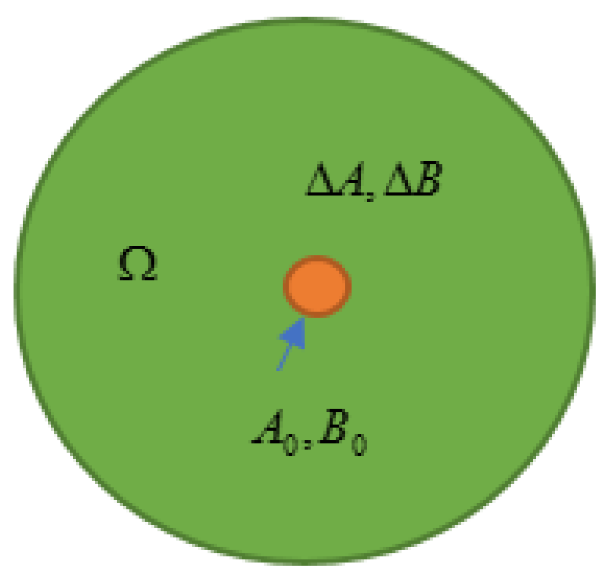
From the above, there is an implicit precondition that the uncertainty domain surrounds the normal system parameter value, that is, the nominal parameter value is used to design a guaranteed robust cost controller, as shown in Figure 1.

Figure 1. Diagram of the uncertainty domain.

As more fault information becomes available, the uncertainty domain of a fault where the value point of the system parameter vector can be located will become narrower. According to Theorem 1 of progressive optimal fault-tolerant control, the minimum upper bound of performance index (23) continuously decreases until a fault is fully identified or no more fault information can be provided. Furthermore, due to the currently insufficient fault information, the fault-tolerant controller should, at this time, be optimal.

Obviously, after a fault occurs, a system must deviate from the nominal state, and if the nominal parameter value is used to design a progressive optimal fault-tolerant controller, the fault-tolerant control can be conservative or even invalid. Therefore, in this study, domain segmentation is introduced for the uncertainty domain of a fault to obtain the auxiliary center point to design a progressive optimal fault-tolerant controller.

At each time, the uncertainty domain ${\Omega }_i$ of a fault can be determined according to the current and insufficient fault information. Then, domain segmentation is performed on the uncertainty domain ${\Omega }_i$ of the fault. Each sub-domain ${\Omega }_{iw},w=1,2,3,\dots s,i=1,2,3\dots$ of uncertainty domain ${\Omega }_i$ satisfies the condition of ${\Omega }_i={\Omega }_{i1}\cup {\Omega }_{i2}\cup \dots \cup {\Omega }_{iw}\cup \dots \cup {\Omega }_{is},w=1,2,3\dots s,i=1,2,3\dots$, where $s$ represents the number of sub-domains. Then, the center point for each sub-domain ${\Omega }_{iw}$ is selected as an auxiliary center point.

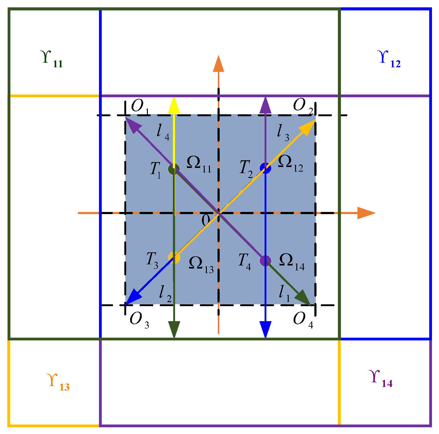
For the auxiliary center points, the farthest distance from each auxiliary center point to the boundary of the current uncertainty domain of a fault is used as the maximum uncertainty magnitude of that point. At each segmentation part for ${\Omega }_i$, there is a different uncertainty domain ${\Upsilon }_{iw},w=1,2,3\dots s,i=1,2,3\dots$ for each auxiliary center point for each sub-domain ${\Omega }_{iw}$. Meanwhile, $s$ is also the number of auxiliary center points. For instance, for the rectangle uncertainty domain ${\Omega }_1$ in Figure 2, grid segmentation is performed on the uncertainty domain, dividing it into four uncertainty sub-domains ${\Omega }_{1w},w=1,2,3,4$. Next, the center point $T_w,w=1,2,3,4$ is selected for each uncertainty sub-domain ${\Omega }_{1w},w=1,2,3,4$ as an auxiliary center point. Then, the length $l_w,w=4,3,2,1$ from the auxiliary center point $T_w,w=1,2,3,4$ to the farthest boundary point $O_w,w=4,3,2,1$ in the whole rectangle uncertainty domain is denoted as the maximum amplitude of square uncertainty domain ${\Upsilon }_{1w},w=1,2,3,4$. Furthermore, controller (21) is designed with the corresponding auxiliary center for each uncertainty domain ${\Upsilon }_{1w},w=1,2,3,4$. Finally, the controllers for all uncertainty domains ${\Upsilon }_{1w},w=1,2,3,4$ form the feasible domain $\Psi ({\Omega }_1)$.

Figure 2. The diagram of the uncertainty domain determination.

Theorem 2.

For the guaranteed robust cost controller vectors $K$ designed for each uncertainty domain ${\Upsilon }_{iw},w=1,2,3\dots s,i=1,2,3\dots$, the controller with the minimum upper bound of the performance index represents a progressive optimal fault-tolerant controller.

$$K=\arg \min (J)=\arg \min (\mathrm{tr}(H))=Y{X}^{-1}$$

(24)

Proof of Theorem 2.

It is obvious that controller $K$ in (21), designed for each uncertainty domain ${\Upsilon }_{iw},w=1,2,3\dots s,i=1,2,3\dots$ is also feasible for ${\Omega }_{iw},w=1,2,3\dots s,i=1,2,3\dots$ due to the fact that ${\Omega }_i={\Upsilon }_{i1}\cap {\Upsilon }_{i2}\cap \dots \cap {\Upsilon }_{iw}\cap \dots \cap {\Upsilon }_{is},w=1,2,3,\dots s,i=1,2,3\dots$. Namely, controllers $K$ in (21), corresponding to the auxiliary center points of ${\Upsilon }_{iw},w=1,2,3\dots s,i=1,2,3\dots$, form a feasible domain $\Psi ({\Omega }_i)$ on ${\Omega }_i$. Thus, controller (24), with the minimum upper bound of performance index (23) in the feasible domain $\Psi ({\Omega }_i)$, denotes the current progressive optimal fault-tolerant controller. □

As the uncertainty domain of a fault decreases with the progressive increase in the sufficiency of the fault information, the aim is to find a progressive optimal fault-tolerant controller corresponding to (24) in the feasible domain $\Psi ({\Omega }_i)$ to achieve progressive optimal fault-tolerant control. The progressive optimal fault-tolerant control process based on a guaranteed robust cost control considers both stability and performance simultaneously.

3.2. Progressive Optimal Fault-Tolerant Algorithm

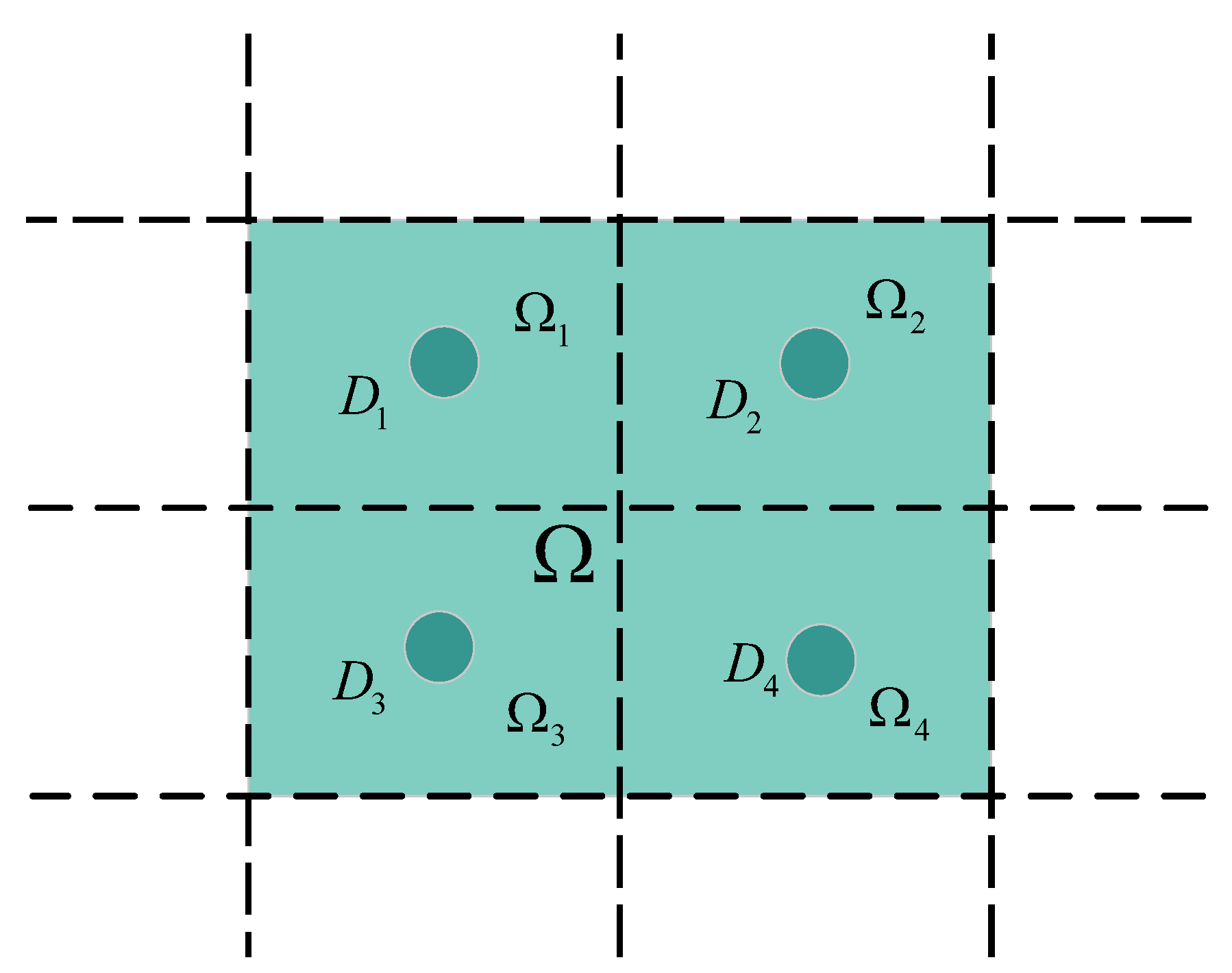
From the above, it is necessary to segment the uncertainty domain of a fault and set the auxiliary center point to design a progressive optimal fault-tolerant control algorithm according to the aforementioned control method. Furthermore, to determine the center point for each segmented domain as an auxiliary center point more easily, grid segmentation is selected as a division method for the uncertainty domains of a fault. The number of grids to be divided is determined according to the specific uncertainty domain. Then, the center points of each grid are regarded as auxiliary center points to design a controller. For the rectangle uncertainty domain $\Omega$ of a fault, as shown in Figure 3, the uncertainty domain $\Omega$ is divided into four grids, denoted by ${\Omega }_1,{\Omega }_2,{\Omega }_3$, and ${\Omega }_4$. The grid center points $D_1–D_4$ of each grid are used as auxiliary center points.

Figure 3. An example of grid segmentation.

The pseudo-code of the progressive optimal fault-tolerant control (Algorithm 1) is presented below.

Algorithm 1. Progressive optimal fault-tolerant control algorithm from the perspective of guaranteed robust cost control.

Input: $A,B$ for $i$ from the first time to the $n\mathrm{th}$ time with an increment of 1  for $w$ form 1 to $s$ with an increment of 1 Assure uncertainty domain ${\Omega }_i$ of faults and perform the grid segmentation on ${\Omega }_i$, dividing it into $s$ uncertainty sub-domains denoted by ${\Omega }_{iw},i=1,2,3,\dots ,n,w=1,2,3,\dots ,s,i=1,2,3\dots$. Use the center points of the grids as auxiliary center points. The farthest distance from the center points of each grid to the boundary of ${\Omega }_i$ is as a maximum uncertainty magnitude of that point. Determine $\Delta A_{iw}$ and $\Delta B_{iw}$ of each uncertainty domain ${\Upsilon }_{iw},w=1,2,3\dots s,i=1,2,3\dots$ and realize the singular value decomposition of $\Delta A_{iw}=M{F}_{1w}(t)E_{1w}$, $\Delta B_{iw}=M{F}_{2w}(t)E_{2w}$;  Solve linear matrix inequality (22) for each grid.  All guaranteed robust cost controllers (21) for each grid form a feasible domain $\Psi ({\Omega }_i)$ on ${\Omega }_i$.  end for  Find the controller $K$ satisfying (24) in $\Psi ({\Omega }_i)$ as the current progressive optimal fault-tolerant controller.  return controller $K$ if no more useful fault information is provided end for end if  return controller $K$ end for

4. Simulations

In the simulation part, the progressive optimal fault-tolerant control of a DC motor with the state space model is considered [37]:

$$\begin{array}{l}\dot{x}=(\mathbf{A}+\Delta A)x+\mathbf{B}u+\mathbf{D}d\\ y=\mathbf{C}x\end{array}$$

(25)

with $x={\left[\begin{array}{cc}{i}_a& \omega \end{array}\right]}^{\mathrm{T}}$ and $\Delta A$ being the uncertainty caused by the parameter fault. The disturbance $d=-\frac{T_l}{J_i}$.

$$\begin{array}{l}A=\left[\begin{array}{cc}-\frac{R_a}{L_a}& -\frac{K_v}{L_a}\\ \frac{K_m}{J_i}& -\frac{G}{J_i}\end{array}\right],B=\left[\begin{array}{c}\frac{1}{L_a}\\ 0\end{array}\right],\\ D=\left[\begin{array}{c}0\\ 1\end{array}\right],C=\left[\begin{array}{cc}1& 0\\ 0& 1\end{array}\right],\Delta A=\left[\begin{array}{cc}0& -\frac{{\mathrm{\sigma }}_v}{L_a}\\ \frac{{\mathrm{\sigma }}_m}{J_i}& 0\end{array}\right]\end{array}$$

(26)

$$u=Kx=[k_1,k_2]x$$

(27)

where $i_a$, $\omega$, and $v_a$ denote the armature current, angular velocity, and armature voltage, respectively. $R_a$ is the armature resistance, and $L_a$ is the inductance of the DC motor. $K_v$ and $K_m$ are the voltage and motor constants, which are supposed to have parameter variations of $\left|{\sigma }_{kv}\right|\le 2$ and $\left|{\sigma }_{km}\right|\le 2$, respectively, due to the fault. $J_i$ is the moment of inertia, and $G$ is the friction coefficient. $K\in {\mathbf{R}}^{1\times 2}$ is the controller parameter vector. $T_l$ is the unknown load torque.

The purpose of the simulation is to regulate the output error of $y$, which represents the armature current and angular velocity error, to be near zero under a fault. The normal parameter values used in the simulations are presented in Table 1.

Table 1. Parameter values [38].

Parameter	Value
$R_a$	1.2 Ω
$L_a$	0.05 mH
$K_v$	0.6
$K_m$	0.6
$J_i$	0.1352 m4
$G$	0.3

The faulty system (28) is considered.

$$A_f=\left[\begin{array}{cc}-\frac{R_a}{L_a}& -\frac{K_v-0.4}{L_a}\\ \frac{K_m+0.6}{J_i}& -\frac{G}{J_i}\end{array}\right],B=\left[\begin{array}{c}\frac{1}{L_a}\\ 0\end{array}\right],D=\left[\begin{array}{c}0\\ 1\end{array}\right],C=\left[\begin{array}{cc}1& 0\\ 0& 1\end{array}\right]$$

(28)

Then, the below algorithm is performed:

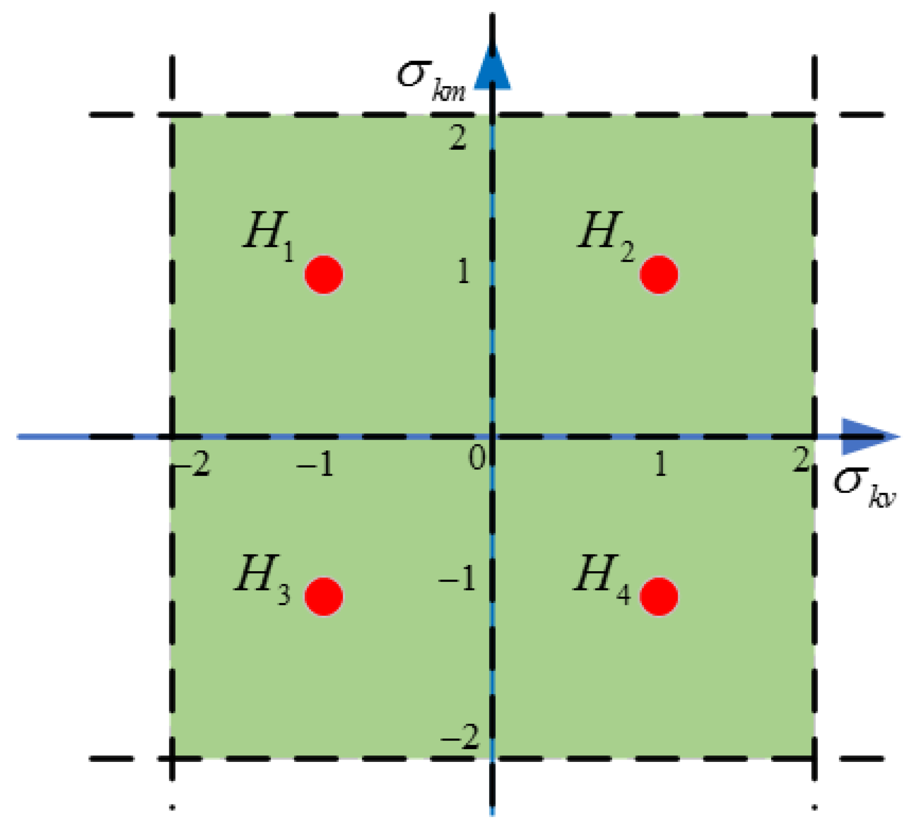
Case 1: After a parametric fault occurs, the maximum uncertainty domain can be assured according to prior knowledge, and $\Delta A_1=\left[\begin{array}{cc}0& -\frac{\left|2\right|}{L_a}\\ \frac{\left|2\right|}{J_i}& 0\end{array}\right]$. ${\sigma }_{kv}=0,{\sigma }_{kv}=2,{\sigma }_{kv}=-2,{\sigma }_{km}=0,{\sigma }_{km}=2,{\sigma }_{km}=-2$ are used to perform grid segmentation on the uncertainty domain, as shown in Figure 4. The center points of the grids, $H_1–H_4$, are used as auxiliary center points. The calculation results corresponding to each auxiliary center point are shown in Table 2, which includes the optimization performance index $\min (J^{*})$ corresponding to the feasible domain of the controller parameter and the progressive optimal fault-tolerant controller.

Figure 4. The grid segmentation in Case 1.

Table 2. The progressive optimal fault-tolerant controller parameters in Case 1.

Auxiliary Center Point	${\mathit{\sigma }}_{\mathit{k}\mathit{v}},{\mathit{\sigma }}_{\mathit{k}\mathit{m}}$	$\mathbf{\Delta }{A}_{\mathbf{1}\mathit{r}}(\mathit{r}=1,2,3,4)$	$K\mathit{n}(\mathit{n}=1,2,3,4)$	${\mathit{J}}_1^{*}$	$\mathbf{min}({\mathit{J}}_1^{*})$	Progressive Optimal Controller
(1,1)	$-3\le {\sigma }_{kv}\le 1$ $-3\le {\sigma }_{km}\le 1$	$\left[\begin{array}{cc}0& -\frac{-3}{L_a}\\ \frac{-3}{J_i}& 0\end{array}\right]$	$K1=$ [−0.0912,0.0020]	15.2337	15.2337	$K1=$ [−0.0912,0.0020]
(−1,1)	$-1\le {\sigma }_{kv}\le 3$ $-3\le {\sigma }_{km}\le 1$	$\left[\begin{array}{cc}0& -\frac{3}{L_a}\\ \frac{-3}{J_i}& 0\end{array}\right]$	$K2=$ [0.2630,0.5141]	36.4675
(−1,−1)	$-1\le {\sigma }_{kv}\le 3$ $-1\le {\sigma }_{km}\le 3$	$\left[\begin{array}{cc}0& -\frac{3}{L_a}\\ \frac{3}{J_i}& 0\end{array}\right]$	$K3=$ [0.0084,−0.0503]	32.9878
(1,−1)	$-3\le {\sigma }_{kv}\le 1$ $-1\le {\sigma }_{km}\le 3$	$\left[\begin{array}{cc}0& -\frac{-3}{L_a}\\ \frac{3}{J_i}& 0\end{array}\right]$	$K4=$ [0.2203,−1.7682]	34.5717

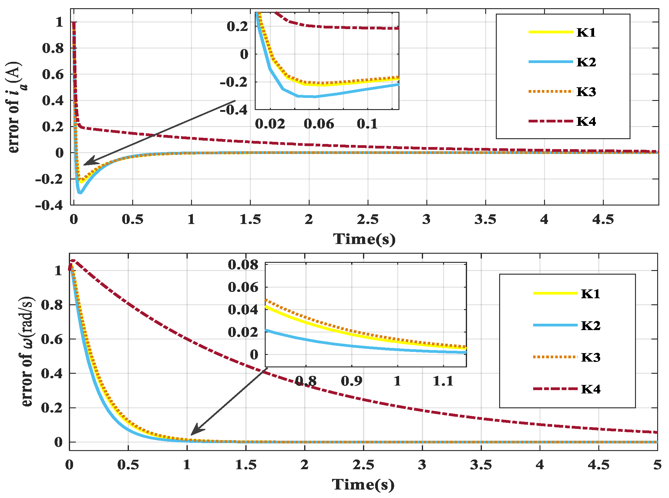
The fault-tolerant control result of Case 1, obtained using fault-tolerant controllers $K1$, $K2$, $K3$, and $K4$, is shown in Figure 5. Based on Table 2, the optimal progressive optimal fault-tolerant controller is $K1$, with a minimum upper bound of optimization performance index of $\min (J_1^{*})=15.2337$, compared to $K2$ with $J_1^{*}=36.4675$, $K3$ with $J_1^{*}=32.9878$, and $K4$ with $J_1^{*}=34.5717$. As shown in Figure 5, controller $K1$ performs better than controllers $K2$, $K3$, and $K4$, with less overshooting and better comprehensive performance.

Figure 5. The control result of Case 1.

Case 2: In this case, it is assumed that the uncertainty domain narrows with the increase in the amount of fault information, and $\Delta A_2=\left[\begin{array}{cc}0& -\frac{\left|1\right|}{L_a}\\ \frac{\left|1\right|}{J_i}& 0\end{array}\right]$. Furthermore, ${\sigma }_{kv}=0,{\sigma }_{kv}=1,{\sigma }_{kv}=-1,{\sigma }_{km}=0,{\sigma }_{km}=1,{\sigma }_{km}=-1$ are used to perform grid segmentation on the uncertainty domain, as shown in Figure 6. The center points of the grids, $D_1–D_4$, are used as auxiliary center points. The calculation results corresponding to each auxiliary center point are shown in Table 3, which includes the optimization performance index $\min (J^{*})$ corresponding to the feasible domain of the controller parameter and the progressive optimal fault-tolerant controller.

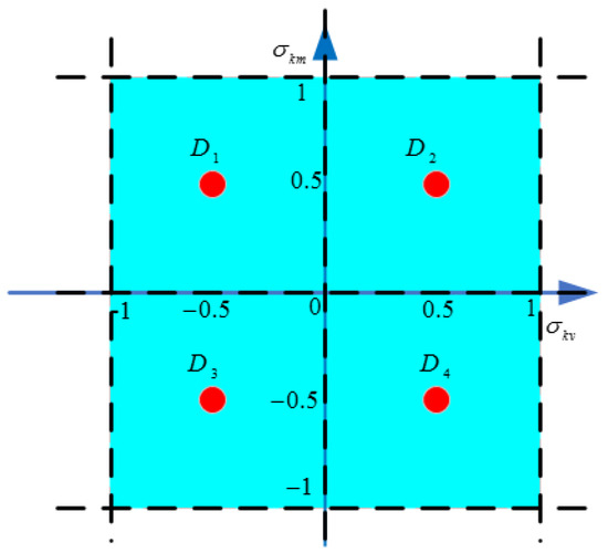
Figure 6. The grid segmentation in Case 2.

Table 3. The progressive optimal fault-tolerant controller parameters in Case 2.

Auxiliary Center Point	${\mathit{\sigma }}_{\mathit{k}\mathit{v}},{\mathit{\sigma }}_{\mathit{k}\mathit{m}}$	$\mathbf{\Delta }{A}_{2\mathit{r}}(\mathit{r}=1,2,3,4)$	$K\mathit{n}(\mathit{n}=5,6,7,8)$	${\mathit{J}}_2^{*}$	$\mathbf{min}({\mathit{J}}_2^{*})$	Progressive Optimal Controller
(0.5,0.5)	$-1.5\le {\sigma }_{kv}\le 0.5$ $-1.5\le {\sigma }_{km}\le 0.5$	$\left[\begin{array}{cc}0& -\frac{-1.5}{L_a}\\ \frac{-1.5}{J_i}& 0\end{array}\right]$	$K5=$ [−0.2389,−0.1059]	9.7222	9.7222	$K5=$ [−0.2389,−0.1059]
(−0.5,0.5)	$-0.5\le {\sigma }_{kv}\le 1.5$ $-1.5\le {\sigma }_{km}\le 0.5$	$\left[\begin{array}{cc}0& -\frac{1.5}{L_a}\\ \frac{-1.5}{J_i}& 0\end{array}\right]$	$K6=$ [0.1685,0.1665]	18.8913
(−0.5,−0.5)	$-0.5\le {\sigma }_{kv}\le 1.5$ $-0.5\le {\sigma }_{km}\le 1.5$	$\left[\begin{array}{cc}0& -\frac{1.5}{L_a}\\ \frac{1.5}{J_i}& 0\end{array}\right]$	$K7=$ [0.0547,0.0400]	22.6618
(0.5,−0.5)	$-1.5\le {\sigma }_{kv}\le 0.5$ $-0.5\le {\sigma }_{km}\le 1.5$	$\left[\begin{array}{cc}0& -\frac{-1.5}{L_a}\\ \frac{1.5}{J_i}& 0\end{array}\right]$	$K8=$ [0.0187,0.0543]	44.2438

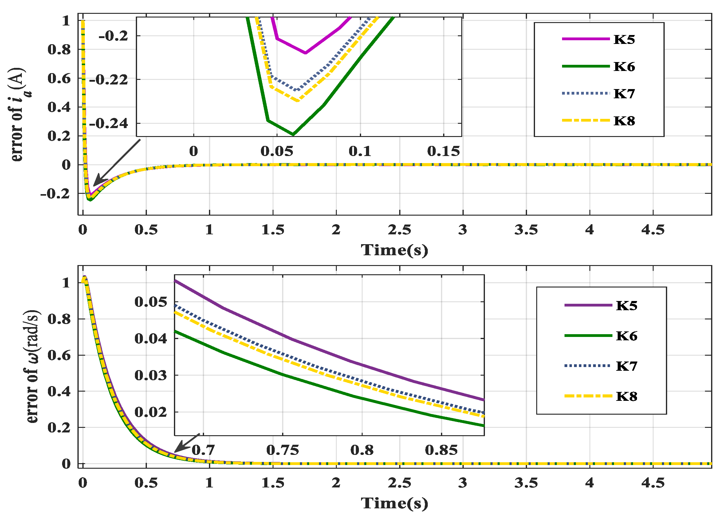
The fault-tolerant control result of Case 2, obtained using fault-tolerant controllers ${\rm K}5$, $K6$, $K7$, and $K8$, is shown in Figure 7. Based on Table 3, the optimal progressive optimal fault-tolerant controller is $K5$, with a minimum upper bound of optimization performance index of $\min (J_2^{*})=9.7222$, compared to $K6$ with $J_2^{*}=18.8913$, $K7$ with $J_2^{*}=22.6618$, and $K8$ with $J_2^{*}=44.2438$. As shown in Figure 7, controller $K5$ performs better than controllers $K6$, $K7$, and $K8$, with less overshooting and better comprehensive performance.

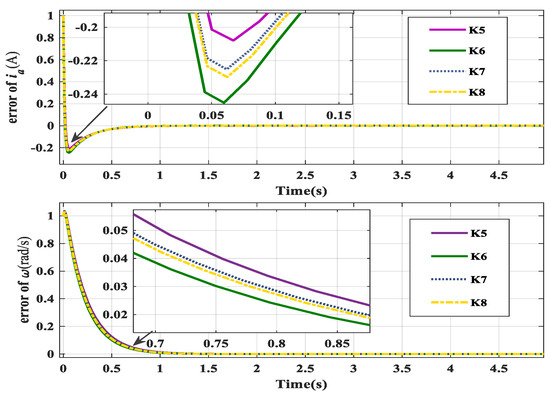
Figure 7. The control result of Case 2.

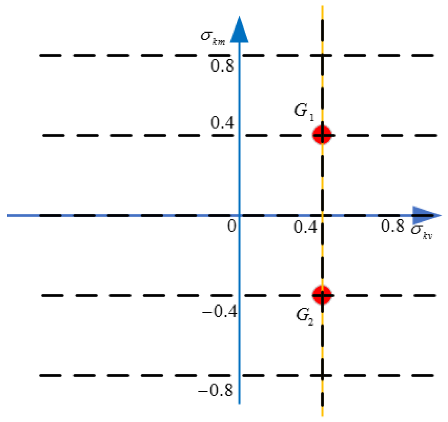
Case 3: In this case, it is assumed that the uncertainty domain decreases with the increase in the amount of fault information and that a fault parameter has been identified, that is, ${\sigma }_{3v}=0$. Then, it follows that $\Delta A_3=\left[\begin{array}{cc}0& 0\\ \frac{\left|0.8\right|}{J_i}& 0\end{array}\right]$. Furthermore, ${\sigma }_{kv}=0.4,{\sigma }_{km}=0,{\sigma }_{km}=0.8,{\sigma }_{km}=-0.8$ are used to perform grid segmentation on the uncertainty domain, as shown in Figure 8. The center points of the grids, $G_1$ and $G_2$, are used as auxiliary center points. The calculation results corresponding to each auxiliary center point are shown in Table 4, which includes the optimization performance index $\min (J^{*})$ corresponding to the feasible domain of the controller parameter and the progressive optimal fault-tolerant controller.

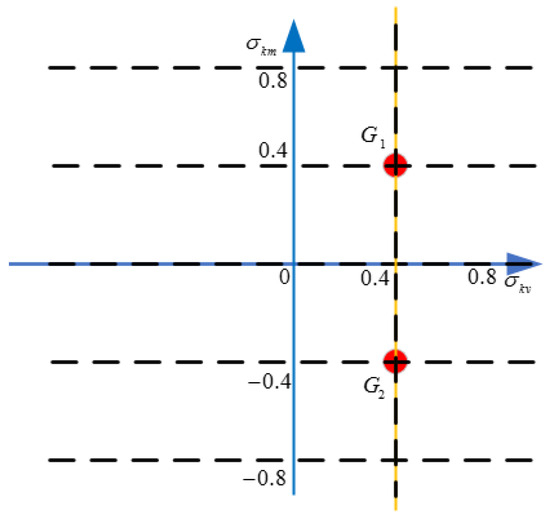
Figure 8. The grid segmentation in Case 3.

Table 4. The progressive optimal fault-tolerant controller parameters in Case 3.

Auxiliary Center Point	${\mathit{\sigma }}_{\mathit{k}\mathit{v}},{\mathit{\sigma }}_{\mathit{k}\mathit{m}}$	$\mathbf{\Delta }{A}_{3\mathit{r}}(\mathit{r}=1,2)$	$K\mathit{n}(\mathit{n}=9,10)$	${\mathit{J}}_3^{*}$	$\mathbf{min}({\mathit{J}}_3^{*})$	Progressively Optimal Controller
(0.4,0.4)	${\sigma }_{kv}=0$ $-1.2\le {\sigma }_{km}\le 0.4$	$\left[\begin{array}{cc}0& 0\\ \frac{-1.2}{J_i}& 0\end{array}\right]$	$K9=$ [−0.4347,−0.2762]	6.8313	6.8313	$K9=$ [−0.4347,−0.2762]
(0.4,−0.4)	${\sigma }_{kv}=0$ $-0.4\le {\sigma }_{km}\le 1.2$	$\left[\begin{array}{cc}0& 0\\ \frac{1.2}{J_i}& 0\end{array}\right]$	$K10=$ [−0.2968,−0.2409]	10.2335

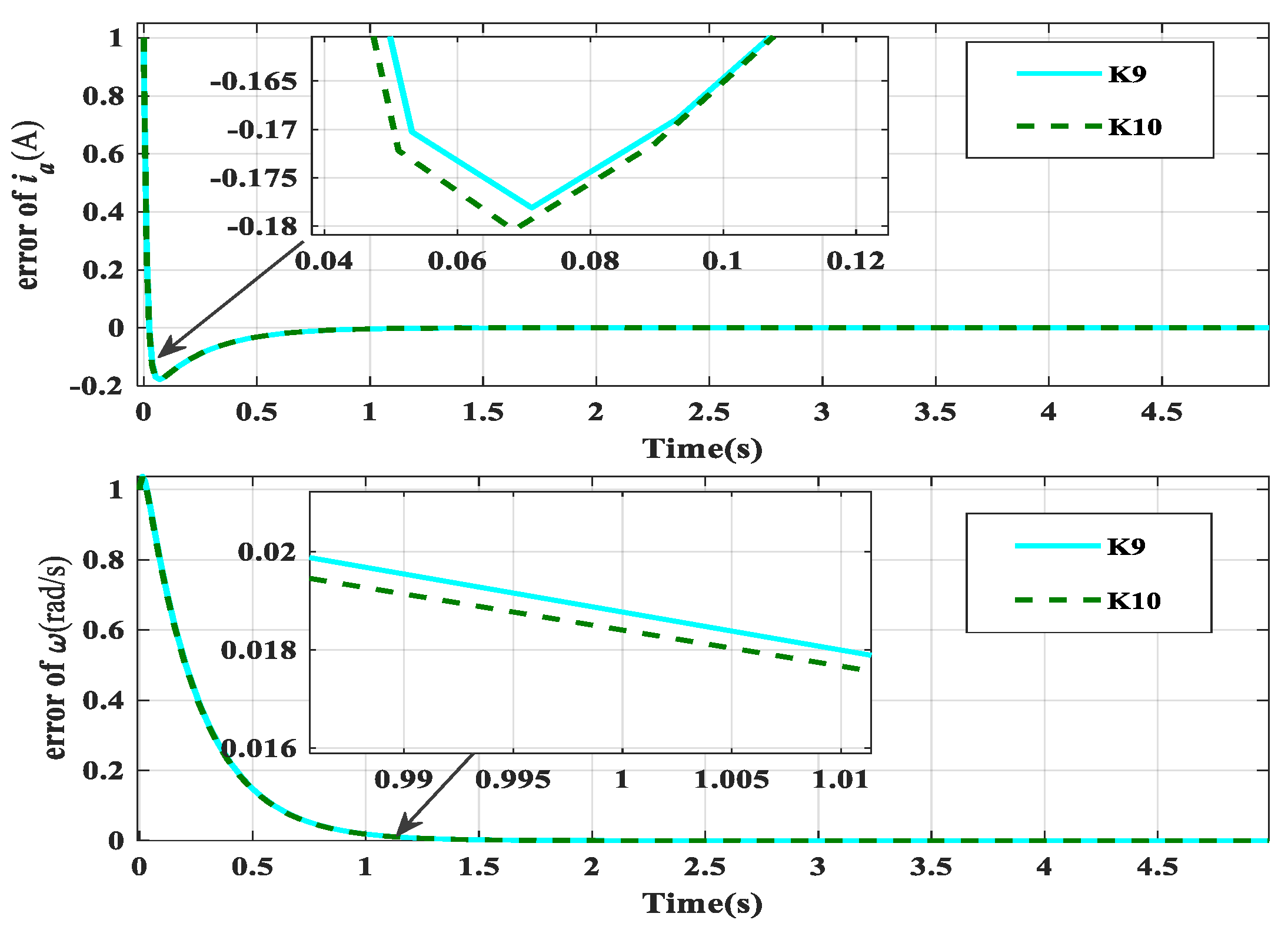
The fault-tolerant control result of Case 3, obtained using fault-tolerant controllers $K9$ and $K10$, is shown in Figure 9. Based on Table 4, the optimal progressive optimal fault-tolerant controller is $K9$, with a minimum upper bound of the performance index of $\min (J_3^{*})=6.8313$, compared to $K10$ with $J_3^{*}=10.2335$. As shown in Figure 9, controller $K9$ performs better than controller $K10$, having less overshooting and better comprehensive performance.

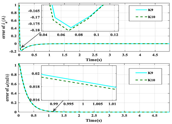
Figure 9. The control result of Case 3.

According to the data presented in Table 2, Table 3 and Table 4 the minimum upper bound $\min (J^{*})$ of the performance index decreases as the uncertainty domain becomes narrower. It is $\min ({J_1}^{*})=15.2337$ for $\Delta A_1=\left[\begin{array}{cc}0& -\frac{\left|2\right|}{L_a}\\ \frac{\left|2\right|}{J_i}& 0\end{array}\right]$, $\min ({J_2}^{*})=9.7222$ for $\Delta A_2=\left[\begin{array}{cc}0& -\frac{\left|1\right|}{L_a}\\ \frac{\left|1\right|}{J_i}& 0\end{array}\right]$, and $\min ({J_3}^{*})=6.83134$ for $\Delta A_3=\left[\begin{array}{cc}0& 0\\ \frac{\left|0.8\right|}{J_i}& 0\end{array}\right]$, which meets the theory of progressive optimal fault-tolerant control. After each grid segmentation of the uncertainty domain, the progressive optimal fault-tolerant controller can be obtained. In addition, the corresponding progressive optimal fault-tolerant controller is optimal before the uncertainty domain stops narrowing, that is, before the amount of useful fault information stops increasing or the fault is identified. The above simulation results also verify the feasibility of the algorithm.

5. Conclusions

This paper presents the progressive optimal fault-tolerant control method, combining the AFTC and PFTC manners by fully using insufficient fault information. In this study, a system fault is considered as system uncertainty. A progressive optimal fault-tolerant control method based on guaranteed robust cost control has been proposed. The proposed method addresses two aspects. First, as the uncertainty domain of the fault parameter becomes narrower, the fault-tolerant effect improves. Second, at each time, based on the uncertainty domain of the corresponding fault information, a currently optimal fault-tolerant controller is determined. In the process of progressive optimal fault-tolerant control, the optimal fault-tolerant controller is no longer reconfigured until no more useful fault information can be provided. Finally, the process of progressive optimal fault-tolerant control converges to active fault-tolerant control once the fault is completely identified. A progressive optimal fault-tolerant control algorithm based on the grid segmentation of the uncertainty domains of a fault and the selection of auxiliary center points has been introduced. The proposed method is validated by a theoretical analysis and simulation. The proposed method has potential application value in practical control systems. In future work, attention will be focused on exploring progressive optimal fault-tolerant control with weaker conservatism and lower computational complexity.

References

- Xiao, B.; Karimi, H.R.; Yu, X.; Gao, Q. IEEE access special section: Recent advances in fault diagnosis and fault-tolerant control of aerospace engineering systems. IEEE Access 2020, 8, 61157–61160. [Google Scholar] [CrossRef]
- Fekih, A. Fault diagnosis and fault tolerant control design for aerospace systems: A bibliographical review. In Proceedings of the American Control Conference, Portland, OR, USA, 4–6 June 2014. [Google Scholar]
- Castaldi, P.; Mimmo, N.; Simani, S. Fault diagnosis and fault tolerant control strategies for aerospace systems. In Proceedings of the 3rd Conference on Control and Fault-Tolerant Systems, Barcelona, Spain, 7–9 September 2016. [Google Scholar]
- Liu, H.; Loh, P.C.; Blaabjerg, F. Review of fault diagnosis and fault-tolerant control for modular multilevel converter of HVDC. In Proceedings of the 39th Annual Conference of Industrial Electronics Society, Vienna, Austria, 10–13 November 2013. [Google Scholar]
- Pazouki, E.; Sozer, Y.; De Abreu-Garcia, J.A. Fault diagnosis and fault-tolerant control operation of non-isolated DC–DC converters. IEEE Trans. Ind. Appl. 2017, 54, 310–320. [Google Scholar] [CrossRef]
- Khan, S.S.; Wen, H. A comprehensive review of fault diagnosis and tolerant control in DC-DC converters for DC microgrids. IEEE Access 2021, 9, 80100–80127. [Google Scholar] [CrossRef]
- Mao, Z.; Yan, X.G.; Jiang, B.; Chen, M. Adaptive fault-tolerant sliding-mode control for high-speed trains with actuator faults and uncertainties. IEEE Trans. Intell. Transp. Syst. 2019, 21, 2449–2460. [Google Scholar] [CrossRef]
- Zhai, M.; Long, Z.; Li, X. Fault-tolerant control of magnetic levitation system based on state observer in high speed maglev train. IEEE Access 2019, 7, 31624–31633. [Google Scholar] [CrossRef]
- Dong, H.; Lin, X.; Gao, S.; Cai, B.; Ning, B. Neural networks-based sliding mode fault-tolerant control for high-speed trains with bounded parameters and actuator faults. IEEE Trans. Veh. Technol. 2019, 69, 1353–1362. [Google Scholar] [CrossRef]
- Liu, S.; Jiang, B.; Mao, Z.; Ding, S.X. Adaptive backstepping based fault-tolerant control for high-speed trains with actuator faults. Int. J. Contr Autom. Syst. 2019, 17, 1408–1420. [Google Scholar] [CrossRef]
- Yao, X.; Li, S.; Li, X. Composite adaptive anti-disturbance fault tolerant control of high-speed trains with multiple disturbances. IEEE Trans. Intell. Transp. Syst. 2022, 23, 21799–21809. [Google Scholar] [CrossRef]
- Zhang, Z.; Ye, D.; Xiao, B.; Sun, Z. Third-order sliding mode fault-tolerant control for satellites based on iterative learning observer. Asian J. Contr. 2019, 21, 43–51. [Google Scholar] [CrossRef]
- Liu, M.; Zhang, A.; Xiao, B. Velocity-Free State Feedback Fault-Tolerant Control for Satellite with Actuator and Sensor Faults. Symmetry 2022, 14, 157. [Google Scholar] [CrossRef]
- Patton, R.J. Robust model-based fault diagnosis: The state of the art. IFAC Proc. Vol. 1994, 27, 1–24. [Google Scholar] [CrossRef]
- Leonhardt, S.; Ayoubi, M. Methods of fault diagnosis. Control. Eng. Pract. 1997, 5, 683–692. [Google Scholar] [CrossRef]
- Simani, S.; Fantuzzi, C.; Patton, R.J. Model-Based Fault Diagnosis Techniques; Springer: London, UK, 2003; pp. 19–60. [Google Scholar]
- Zhang, T.; Chen, J.; Li, F.; Zhang, K.; Lv, H.; He, S.; Xu, E. Intelligent fault diagnosis of machines with small & imbalanced data: A state-of-the-art review and possible extensions. ISA Trans. 2022, 119, 152–171. [Google Scholar] [PubMed]
- Zhou, S.; Wang, K.; Shan, J.; Bao, D.; Hou, Z.; Yanda, L. Data-Driven Multi-Type and Multi-Level Fault Diagnosis of Proton Exchange Membrane Fuel Cell Systems Using Artificial Intelligence Algorithms. SAE Tech. Pap. 2022, 1, 693. [Google Scholar]
- Chang, Y.; Chen, Q.; Chen, J.; He, S.; Li, F.; Zhou, Z. Intelligent fault diagnosis scheme via multi-module supervised-learning network with essential features capture-regulation strategy. ISA Trans. 2022, 129, 459–475. [Google Scholar] [CrossRef]
- Patton, R.J.; Chen, J.; Chen, J. A study on neuro-fuzzy systems for fault diagnosis. Int. J. Syst. Sci. 2000, 31, 1441–1448. [Google Scholar] [CrossRef]
- Jiang, J.; Yu, X. Fault-tolerant control systems: A comparative study between active and passive approaches. Annu. Rev. Control 2012, 36, 60–72. [Google Scholar] [CrossRef]
- Abbaspour, A.; Mokhtari, S.; Sargolzaei, A.; Yen, K.K. A survey on active fault-tolerant control systems. Electronics 2020, 9, 1513. [Google Scholar] [CrossRef]
- Bavili, R.E.; Mohammadzadeh, A.; Tavoosi, J.; Mobayen, S.; Assawinchaichote, W.; Asad, J.H.; Mosavi, A.H. A new active fault tolerant control system: Predictive online fault estimation. IEEE Access 2021, 9, 118461–118471. [Google Scholar] [CrossRef]
- Zhou, H.; Ye, H.; Wu, M. Fault Detection and Fault-Tolerant Control Based on Sliding Mode Theory; National Defence Industry Press: Beijing, China, 2014; pp. 2–25. [Google Scholar]
- Yu, X.; Jiang, J. Hybrid fault-tolerant flight control system design against partial actuator failures. IEEE Trans. Control Syst. Technol. 2011, 20, 871–886. [Google Scholar] [CrossRef]
- Jiang, J.; Zhao, Q. Fault tolerant control system synthesis using imprecise fault identification and reconfigurable Control. In Proceedings of the IEEE International Symposium on Intelligent Control (ISIC) held jointly with International Symposium on Computational Intelligence in Robotics and Automation (CIRA), Gaithersburg, MD, USA, 14–17 September 1998. [Google Scholar]
- Tu, Y.; Wang, D.; Ding, S.X.; Fu, F.; Li, W. A Reconfiguration-Based Fault-Tolerant Control Method for Nonlinear Uncertain Systems. IEEE Trans. Autom. Contr. 2021, 61, 6060–6067. [Google Scholar] [CrossRef]
- Li, Z.; Dahhou, B. Fault-tolerant control Based on Insufficient Fault Information. J. Nanjing Univ. Sci. Technol. 2011, 35, 52–55. [Google Scholar]
- Li, Z.; Dahhou, B. An observers based fault isolation approach for nonlinear dynamic systems. In Proceedings of the 2nd International Symposium on Communications, Control and Signal Processing, Marrakech, Morocco, 13–15 March 2006. [Google Scholar]
- Park, Y. Robust and optimal attitude control of spacecraft with disturbances. Int. J. Syst. Sci. 2015, 46, 1222–1233. [Google Scholar] [CrossRef]
- Pan, H.; Xin, M. Nonlinear robust and optimal control of robot manipulators. Nonlinear Dyn. 2014, 76, 237–254. [Google Scholar] [CrossRef]
- Lao, Y.; Scruggs, J.T. Robust control of wave energy converters using unstructured uncertainty. In Proceedings of the American Control Conference (ACC), Denver, CO, USA, 1–3 July 2020. [Google Scholar]
- Cao, Z.; Xiao, Q.; Huang, R.; Zhou, M. Robust neuro-optimal control of underactuated snake robots with experience replay. IEEE Trans. Neural Netw. Learn. Syst. 2017, 29, 208–217. [Google Scholar] [CrossRef] [PubMed]
- Mystkowski, A.; Koszewnik, A.P. Mu-Synthesis robust control of 3D bar structure vibration using piezo-stack actuators. Mech. Syst. Signal Process. 2016, 78, 18–27. [Google Scholar] [CrossRef]
- Xue, A. Robust And Optimal Control Theory and Application; Science Press: Beijing, China, 2008; pp. 15–130. [Google Scholar]
- Gao, Z.; Cecati, C.; Ding, S.X. A survey of fault diagnosis and fault-tolerant techniques-Part I: Fault diagnosis with model-based and signal-based approaches. IEEE Trans. Ind. Electron. 2015, 62, 3757–3767. [Google Scholar] [CrossRef]
- Lan, J.; Patton, R.J. A new strategy for integration of fault estimation within fault-tolerant Control. Automatica 2016, 69, 48–59. [Google Scholar] [CrossRef]
- Belanger, P.R. Control Engineering: A Modern Approach; Oxford University Press: Oxford, UK, 1995; pp. 12–200. [Google Scholar]
Disclaimer/Publisher’s Note: The statements, opinions and data contained in all publications are solely those of the individual author(s) and contributor(s) and not of MDPI and/or the editor(s). MDPI and/or the editor(s) disclaim responsibility for any injury to people or property resulting from any ideas, methods, instructions or products referred to in the content. |
© 2024 by the authors. Licensee MDPI, Basel, Switzerland. This article is an open access article distributed under the terms and conditions of the Creative Commons Attribution (CC BY) license (https://creativecommons.org/licenses/by/4.0/).