Abstract
This paper introduces a two-tier feedback control law for the path tracking of a mobile robot equipped with N on-axle trailers. Initially, through a recursive design process, the curvature-tracking challenge is converted into stabilizing the joint angles at predefined reference values. This design approach is straightforward and can be easily extended to configurations with multiple trailers. Using input-to-state stability analysis, we demonstrate the asymptotic stability of the closed-loop system, which is structured in cascade form. Furthermore, we reformulate the path-tracking problem as a curvature-planning challenge and propose an algorithm to determine the desired curvature for the tail trailer. The simulation results validate the effectiveness of this novel algorithm in truck-trailer systems.
1. Introduction
The truck-trailer system is a pivotal component of transportation infrastructure [1]. The precise path tracking of these systems is of considerable importance in sectors such as agricultural machinery operations, logistics, and transportation services. Despite their critical role, truck-trailer systems encounter numerous challenges during backward path tracking, such as complex nonlinear kinematics, nonholonomic constraints, structural singularities, and instabilities in reverse motion [2]. Consequently, enhancing autonomous driving technology for these systems is not only technically challenging but is also anticipated to significantly lower transportation costs and improve safety, making it a key focus in current research.
Extensive studies in the literature have explored the modeling of truck-trailer systems, categorizing kinematic models based on the steering mechanisms of the front wheels into differential-driven [3,4,5,6] and car-like models [7,8,9,10]. Furthermore, kinematic models differ in their primary hitching configurations: on-axle (or direct-hooked) systems, where the hitch is centrally positioned on the rear axle of the tractor or the preceding trailer [10,11,12,13], and off-axle (or off-hooked) systems, where the hitch is located behind the rear axle [7,9,14,15]. Figure 1 illustrates a simplified schematic of these models. Notably, the on-axle system is considered a specific case of the off-axle system. However, from a control standpoint, these systems exhibit distinct characteristics and are thus studied separately. This study specifically addresses the backward path tracking of a car-like on-axle robot with N trailers, as depicted in Figure 2.
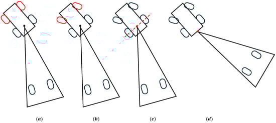
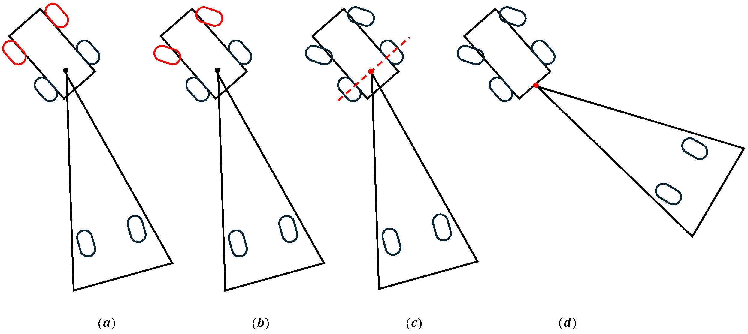
Figure 1.
Four types of truck-trailer model: (a) differential driven steering model, (b) Ackermann steering model, (c) on-axle model with hitch on rear axle, and (d) off-axle model. In models (a,b), red wheels highlight the differences between differential driven and Ackermann steering mechanisms. In models (c,d), red dashed lines distinguish between on-axle and off-axle configurations.
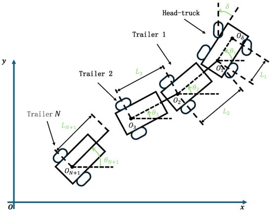
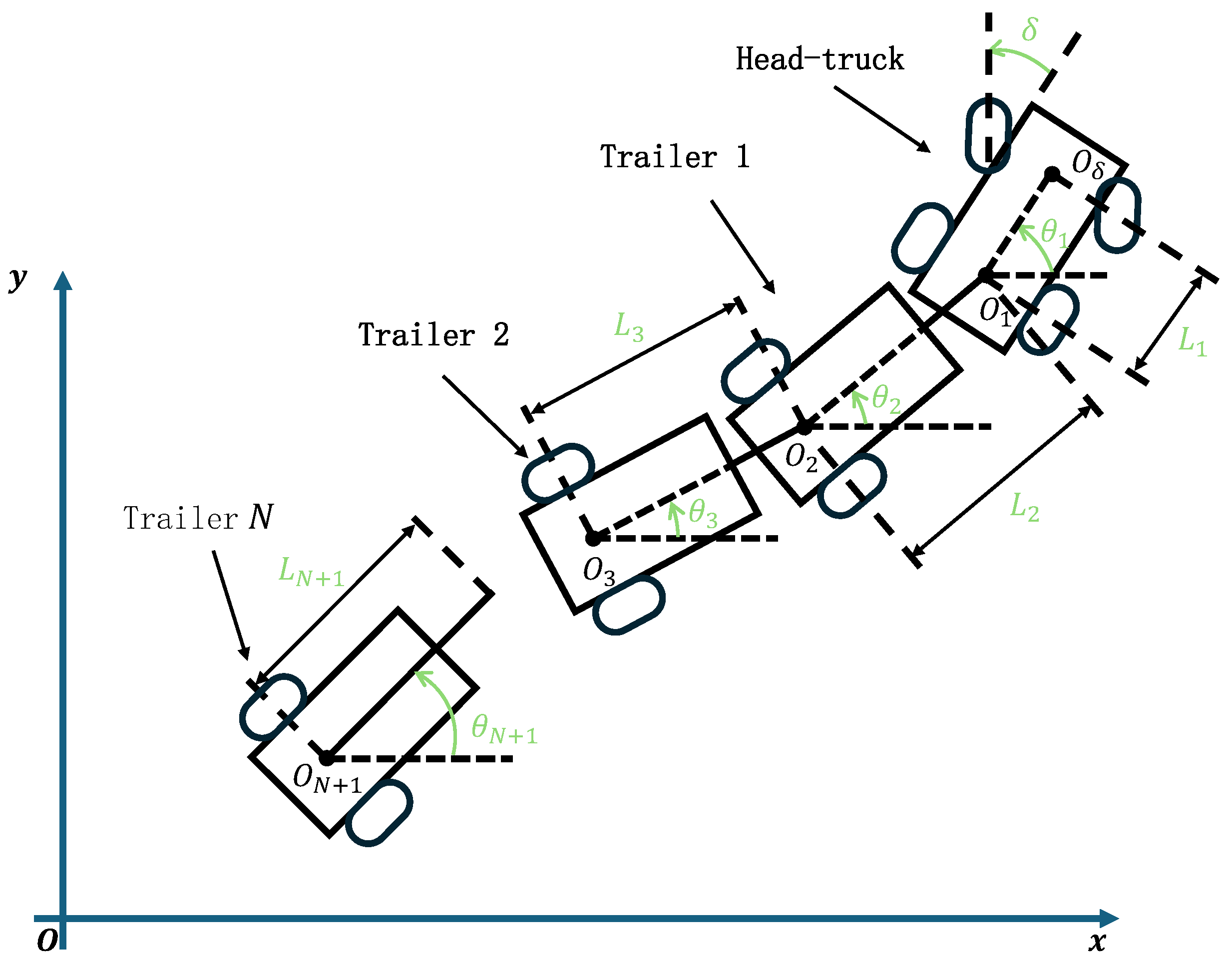
Figure 2.
Geometry of a mobile robot with N trailers.
The development of precise dynamic models for mobile robots is essential for a variety of applications in robotics, automation, and transportation systems. Such models facilitate the accurate analysis and prediction of resistive forces encountered by mobile platforms during movement [3,16,17,18,19,20]. In this paper, following the approach adopted in [10,19,20], we separate kinematic and dynamic controls to achieve backward path tracking for the truck-trailer system. The resulting controller is straightforward and intuitive, and it is specifically designed for low-speed reversing maneuvers. Considering that safety is often prioritized over rapid dynamic performance in reversing scenarios, this separation of control is considered appropriate.
The control problems associated with the truck-trailer system can be categorized into three distinct types: simple tracking [21,22], path tracking [9,10,14,15,23,24], and trajectory tracking [25,26,27,28,29,30]. Simple tracking entails the following of a defined geometric path, such as a circle or straight line, without the requirement to adhere to specific trajectory details. Path tracking involves the truck-trailer system adhering to a predefined path without strict temporal constraints, thereby emphasizing spatial accuracy. In contrast, trajectory tracking demands adherence to a predetermined path with precise timing for reaching designated points, necessitating a careful balance of both spatial and temporal precision.
Among these, simple tracking is restricted to movement along circular or straight-line paths, whereas path and trajectory tracking, which account for environmental constraints, prove more practical in real-world applications. Path tracking is often more crucial than trajectory tracking with rigid time constraints because it allows controllers to focus on maintaining appropriate lateral and longitudinal velocities without the necessity for time synchronization. Additionally, this approach benefits from the time-invariance of the controller, which simplifies the analysis of system stability. This study specifically addresses the issue of backward path-tracking control in mobile robot systems equipped with N trailers.
Research on path-following control for a mobile robot with one trailer has been extensive. For instance, Widyotriatmo explores both forward and backward path following for a truck-trailer system, analyzing performance from two reference points: the head-truck (RH) and the trailer (RT) [10]. The simulation results indicate the superior performance of RT-controls, especially in curve-path following in both directions. Leng discusses a curvature-based method for path tracking, involving the computation of desired tracking curvature and the design of directional control inputs [9,14,15]. Furthermore, Manav has developed an adaptive pure pursuit controller, which was proven to be effective and robust through simulation and experimental validation [31].
Despite these advancements, studies addressing path-following control for mobile robots with multiple trailers (N trailers) remain limited. Ljungqvist proposes a model predictive controller (MPC) for a two-trailer system’s path-tracking problem [32]. Cheng employs fuzzy control technology for a three-trailer system’s path tracking [23] and introduces an orientation tracking controller based on a recursive design process for systems with N trailers [22]. However, these methods are not directly applicable to the broader problem of path following for mobile robots with N trailers.
Building on previous research, this paper presents a novel two-tier curvature-based path-tracking controller for a mobile robot system with N trailers. Initially, the curvature-tracking issue is addressed by stabilizing joint angles to predefined reference values using a recursive design process. Subsequently, a lateral controller, extendable to systems with N trailers, is developed. Through input-to-state stability analysis, the closed-loop system’s cascade representation is shown to be asymptotically stable. The path-following challenge is then reformulated as a curvature-planning issue, and a curvature-planning algorithm for a tail trailer is introduced. The effectiveness of the proposed controller is validated through numerical simulations, confirming its potential applicability in practical scenarios.
The structure of this paper is outlined as follows. In Section 2, we present the kinematic modeling and problem formulation for a truck-trailer system. Section 2.1 elaborates on the kinematic model of a mobile robot with multiple trailers, while Section 2.2 discusses the system properties and formulates the problem. Section 3 proposes a path-following controller, with Section 3.1 detailing the development and theoretical verification of a universal curvature-tracking controller, and Section 3.2 introduces a curvature-planning algorithm designed for tracking the desired path. The efficacy of the proposed path-following controller is validated through numerical simulations in Section 4. The paper concludes in Section 6.
2. Vehicle Kinematic and Problem Statement
The truck-trailer system is a multi-rigid body system. This paper investigates the control of backward movement in such a system by analyzing the kinematic model, where the control inputs are the truck’s traction speed and the steering angle. Dynamic control for tracking the designed traction speed and steering angle can be realized using a well-known Proportional–Integral–Derivative (PID) controller in the dynamics model and detailed in sources such as [19,20]. However, the limitation of separating kinematic and dynamic control lies in the necessity to keep the frequency of the kinematic system lower than that of the dynamic system, allowing the dynamic controls to drive the traction and steering motors effectively to follow the designed speed and steering angles. This section derives the kinematic model for the backward movement of the truck-trailer system. It is assumed that the velocity of the truck-trailer in the direction perpendicular to the surface is always zero.
2.1. Kinematic Model
The kinematic configuration of a mobile robot with N trailers is illustrated in Figure 2, where denotes the center of the truck’s front axle. The truck, functioning as a car-like mobile robot, is propelled by its rear wheels at a linear speed . The steering angle , which represents the angle between the front wheels and the truck’s longitudinal axis, indicates left turns for and right turns for . The system includes an arbitrary number N of passive trailers, which are each sequentially connected to the axle of the vehicle ahead using an on-axle mounting approach. The orientations (where i ranges from 1 to ) of both the tractor and trailers relative to the x-axis are noted. The Cartesian coordinates (for i ranging from 1 to ) pinpoint the center of the rear axle for each tractor and trailer. The joint angles (for i ranging from 1 to N) are defined as (for i ranging from 1 to N). The parameter specifies the length of the tractor’s wheelbase, while (for i ranging from 2 to ) denotes the lengths of the connecting links of the passive trailers.
Derived from the assumption of no-slip motion between the wheels and the ground in a planar environment, the kinematic model of the mobile robot with N trailers can be articulated. Governed by differential equations, the kinematic behavior is encapsulated as follows:
where (for i ranging from 1 to N). In this system formulation (1), the linear speed and steering angle are considered as the control inputs.
2.2. Preliminaries and Problem Formulation
After detailing the kinematic model of the mobile robot system, we now turn our attention to understanding its inherent properties. This comprehension is essential for the development of effective path-following controllers. Initially, this section outlines these properties, providing critical insights needed for controller design.
Property 1.
Structural Singularity. In a standard configuration, the system exhibits a nonholonomy degree of , assuming that . Conversely, if , the maximum degree of nonholonomy corresponds to the -th term in Fibonacci’s sequence [22,33].
A significant implication of this singularity is that the dynamics of become uncontrollable when , for [22].
Property 2.
Instability in Backward Motion. When the robot operates in reverse at a linear speed , the dynamics of show open-loop instability for , where [22].
As noted earlier, a mobile robot system with multiple trailers must address practical constraints to mitigate dynamic singularities and prevent self-collision in real-world scenarios. These constraints are further discussed in the following section. Additionally, instability during reverse motion can induce the “jackknife” phenomenon, where increasing articulated angles between adjacent trailers may cause the vehicle to fold onto itself, potentially leading to a loss of control and collisions. This issue poses significant challenges for path-tracking control in reverse operation scenarios.
The subsequent analysis introduces a mathematical formulation of the research problem tackled in this paper, focusing on backward path-tracking control for a mobile robot with multiple trailers. The problem is divided into two subproblems, which are detailed as follows:
Problem 1.
Curvature-Tracking Control. For the system described in (1), the objective is to derive a feedback control law for δ that enables the tail trailer to track a desired reversing curvature . This requires ensuring that the curvature-tracking error of the tail trailer, defined as , where κ represents the curvature of the tail trailer, asymptotically converges to zero.
Problem 2.
Curvature Planning. For the system described in (1), the aim is to plan the tail trailer’s reversing curvature in such a manner that it facilitates the tracking of the desired path during reverse motion.
3. Path-Tracking Control Law
This section delineates the development of control laws necessary for the reverse motion path following of a truck-trailer system, specifically referencing the tail trailer. In constructing these control laws for backward path following, the following assumptions are established:
Assumption 1
([10,22]). The joint angles (for ), are limited within predefined bounds. Specifically, each angle is constrained such that , where . This constraint arises from the angular limitations of the joint (for ), ensuring that remains positive throughout the motion for all .
Remark 1.
Assumption 1 is deemed reasonable based on its broad acceptance and application in the existing literature, as supported by references such as [10,22]. Additionally, its validity can be ensured through precise hardware design, which allows for the effective control of steering and articulation angles in trailer systems using established hardware mechanisms. This supports the assumption’s practical applicability.
Assumption 2
([10,14,22]). The wheels of the truck-trailer system are assumed to experience neither slipping nor skidding at any point during the motion.
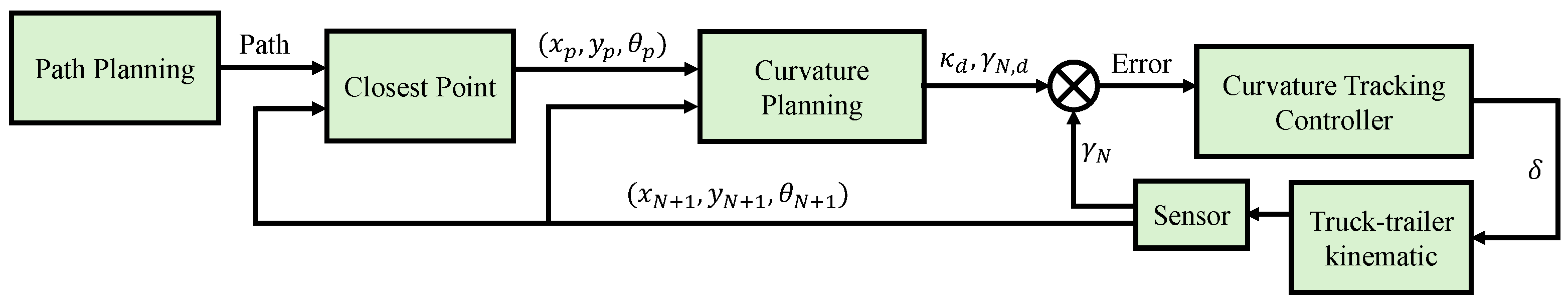
These assumptions streamline the dynamics and control challenges, facilitating a more manageable formulation of the backward path-following control laws. The control strategy proposed in this paper, illustrated in Figure 3, comprises two principal components: one generates the necessary curvature for the tail trailer based on a predefined reference path, and the other computes the steering angle for the head vehicle using a curvature-tracking control law. These components function independently and can be tailored to specific application scenarios. This section initially introduces the curvature-tracking control law and subsequently provides proof of its stability.
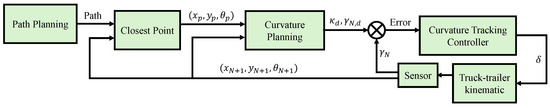
Figure 3.
Control system flowchart for reversing path following of a mobile robot with N trailers.
3.1. Curvature-Tracking Control Law
Firstly, we demonstrate that the curvature-tracking control problem (Problem 1) can be reformulated into stabilizing the articulation angle at a predefined reference value , where represents the desired curvature of the tail trailer.
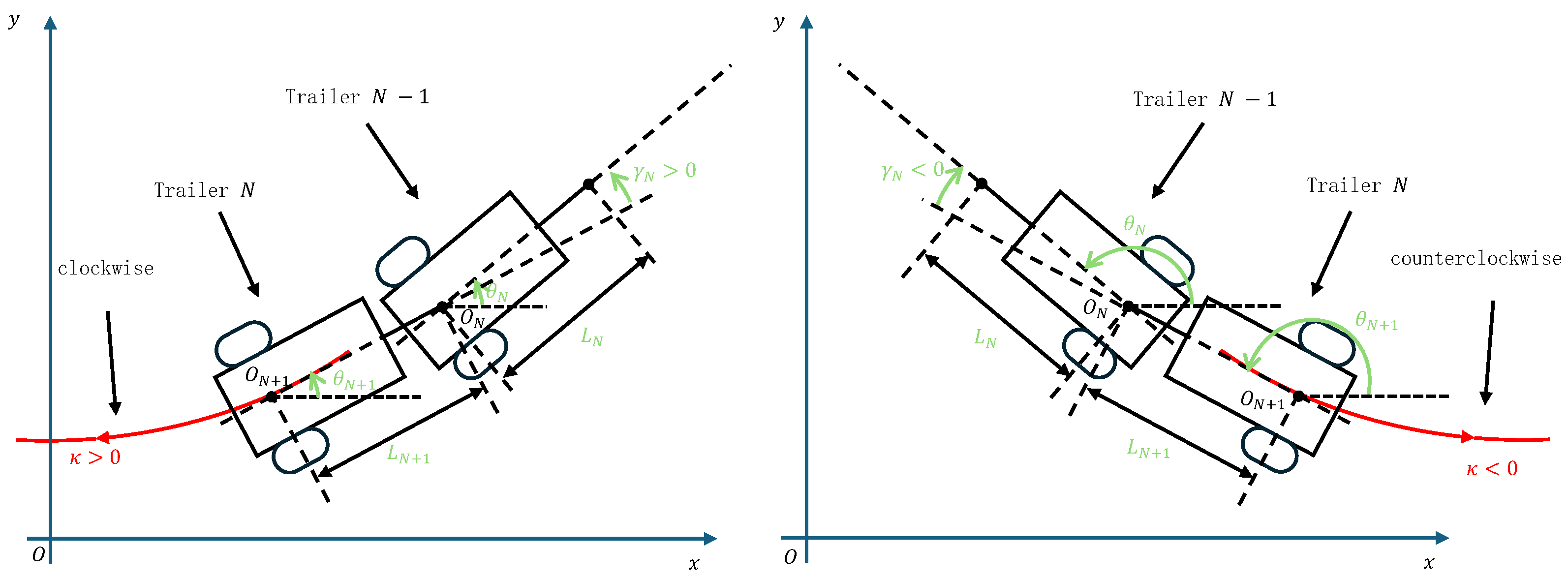
According to the system dynamics shown in Equation (1), the relationship between the trajectory curvature of the tail trailer and the articulation angle is characterized as follows:
If is positive, will also be positive, indicating that the system moves in reverse in a clockwise direction. Conversely, if is negative, will be negative, signifying reverse movement in a counterclockwise direction. Figure 4 visually represents this relationship between and .
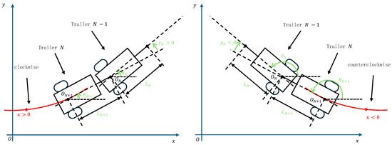
Figure 4.
The relationship between the trajectory curvature and the articulation angle of the tail trailer.
Given Assumption 1, the bounds for are , where , implying that is similarly bounded.
Since the tangent function is monotonic within the interval , there exists a one-to-one correspondence between and . Thus, the problem of tracking the desired curvature translates directly into tracking the reference joint angle , i.e.,
This transformation recasts the curvature-tracking challenge as a control problem centered on the joint angle tracking.
We next delineate the derivation of a control strategy for the joint angle-tracking problem, leveraging the desired joint angle and defining the tracking error as the difference between and , which is expressed as
Using system (1), the derivative of is calculated, leading to
From Equation (5), given the conditions
with , and , it follows that
This implies that will asymptotically converge to zero when t approaches infinity, as demonstrated by the application of the Lyapunov technique.
To maintain consistency with condition (6), define the reference angle for with
and establish the tracking error as
Alongside system (1), the derivative of is derived, showing that
Similar procedures are adopted for defining the reference angle for ,
with an analogous tracking error and its derivative. If converges toward , then
Consequently, will also converge to zero asymptotically as t approaches infinity.
Following this methodological framework, the variables () and reference angles () are recursively designed,
and
where each . From (13), it has
Finally, define the tracking error for the reference angle as
The derivative of along system (1) is expressed by
To ensure the asymptotic stability of at its origin, let
and integrate this into Equation (17) to derive
Consequently, the control law , as designed by (19), facilitates tracking of the desired joint angle in system (1).
The stability of the closed-loop system is established using the concept of input-to-state stability. Consider the following system:
where is piecewise continuous in t and locally Lipschitz in x and u. Here, the control input is characterized as a piecewise continuous, bounded function over .
Definition 1.
System (20) is deemed input-to-state stable if there exists a class function β and a class function δ such that for any initial state and any bounded input , the solution persists for all and satisfies
The definitions of the Class and Class functions are provided in Appendix A. The following lemma offers a convenient method for establishing the input-to-state stability of a system based on the exponential stability of the origin in the corresponding unforced system.
Lemma 1.
Assume the function is continuously differentiable and globally Lipschitz in , uniformly over time t. If the unforced system possesses a globally exponentially stable equilibrium at the origin , then system (20) is input-to-state stable.
Input-to-state stability is instrumental in analyzing the stability of various cascaded and interconnected dynamical systems, as referenced in [34]. Consider a cascade system
where and are piecewise continuous in t and locally Lipschitz in . Assume both
and (23) have globally uniformly asymptotically stable equilibrium points at their respective origins.
Lemma 2.
From Lemma 2, the stability of systems (22) and (23) is secured through the input-to-state stability of subsystem (22) and the asymptotic stability of subsystem (23).
Theorem 1.
Proof.
Considering the control law specified in Equation (19), we employ a Lyapunov candidate function . Since
this yields , indicating that converges to zero asymptotically. As , from Equation (16), approaches .
From Equation (15), we have
Substituting (15) into Equation (26), we obtain
Considering as the input for system (27), systems (27) and (25) are analyzed as a cascade system described by Equations (22) and (23). When , Equation (14) gives
Using another Lyapunov function , we find
ensuring exponential stability for in the unforced system (27). By Lemma 1, system (27) is input-to-state stable. Lemma 2 further confirms that the origin of the cascade system comprising systems (27) and (25) is uniformly asymptotically stable, i.e., and when .
Similarly, for any i from 2 to N, the stability of can be recursively proven. Assuming is asymptotically stable, we observe under this condition. Incorporating as input to subsystem (15) and substituting from (14), it results in
when . Using , we find
confirming that the unforced system (15) is exponentially stable at . By Lemma 1, system (15) is input-to-state stable. Combined with the stability of , it can be concluded that the origin of the cascade system of and is asymptotically stable. For , with , it results in Equation (7). The origin of the cascade system comprising and is also determined to be asymptotically stable, confirming that is asymptotically stable. As each approaches zero, converges to for . □
3.2. Curvature Planning
This section presents a curvature-planning algorithm designed to calculate the desired reference curvature of the tail trailer. The algorithm is based on the current state of the system and a predetermined tracking path with the objective of ensuring precise alignment of the tail trailer with this path during reverse maneuvers.
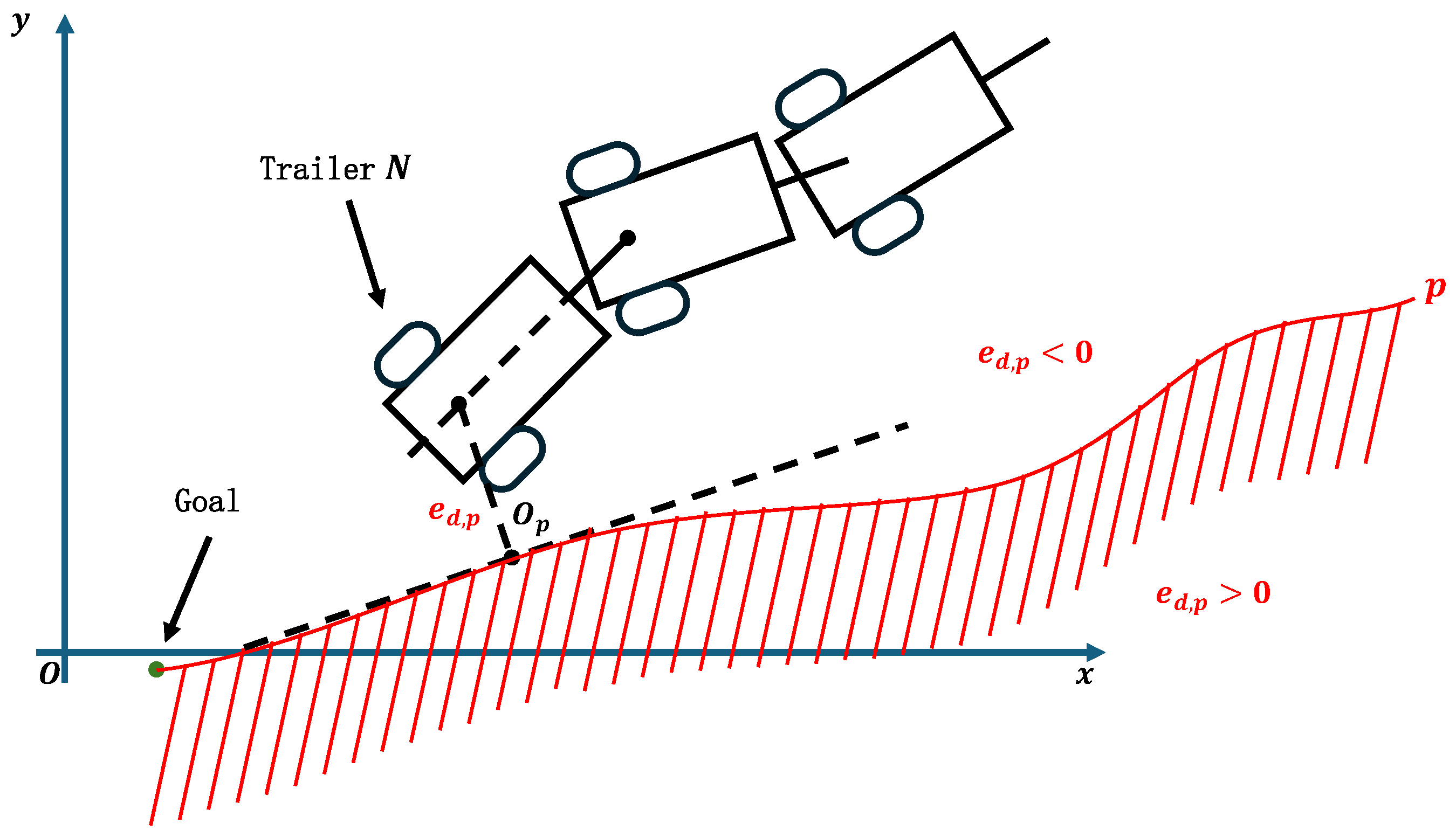
Consider as the point on the desired path that is nearest to the tail trailer at time t. For brevity, the time indicator t will be omitted in subsequent discussions. To resolve potential ambiguities arising from multiple nearest points, p is selected as the point closest to the endpoint of the path in the direction of travel. The coordinates of point p are denoted as , and its orientation angle is denoted as . The path-following schematic for the truck-trailer system is depicted in Figure 5. Additionally, Figure 5 illustrates two critical variables used in path tracking: the orientation error and the distance error . These variables are defined as follows:
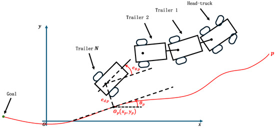
Figure 5.
Schematic of backward motion path following.
The objective of path tracking for the tail trailer involves minimizing both the orientation error and the distance error to zero. To facilitate effective path tracking, we have developed a curvature-planning algorithm, drawing inspiration from the methodology presented in [14]. This algorithm computes the required curvature by integrating three components: the desired path curvature , the orientation tracking curvature , and the distance tracking curvature .
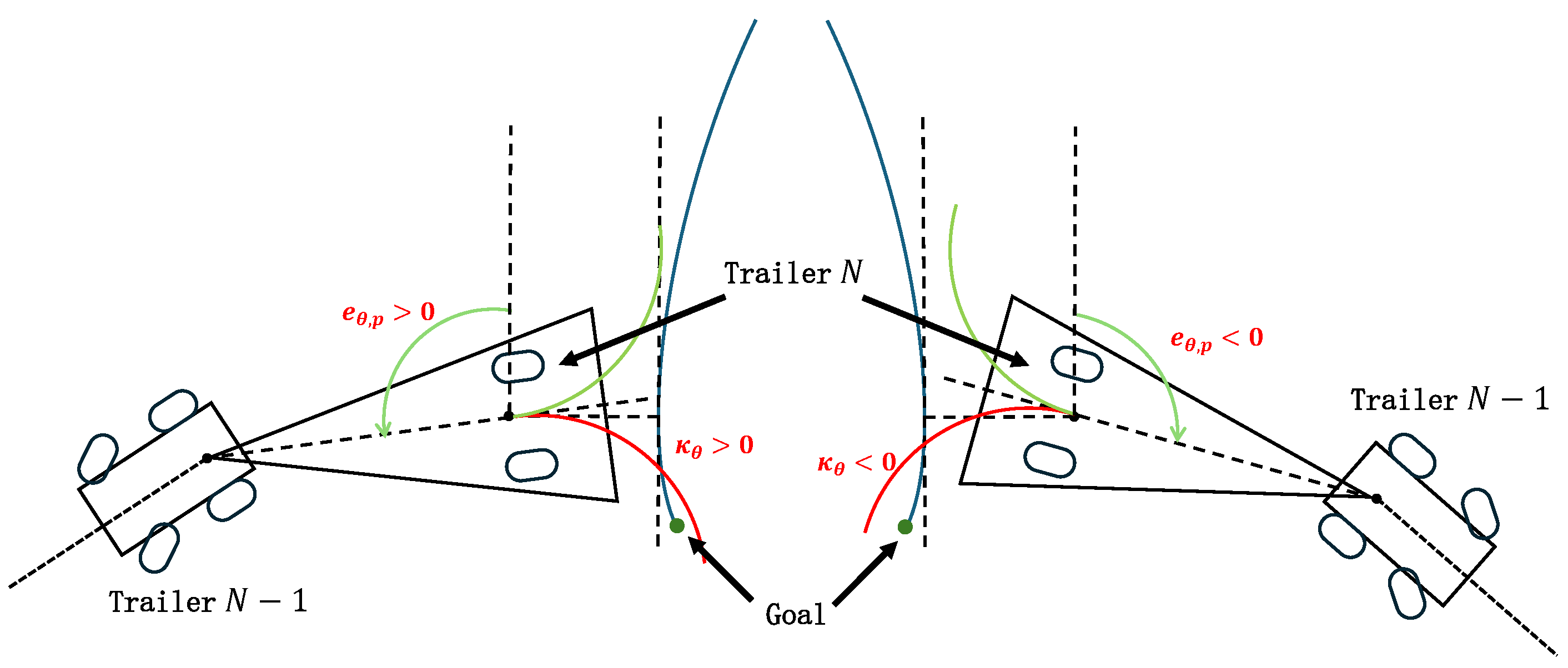
The desired path curvature, , is derived directly from the equation of the curve. For the orientation tracking curvature, , the planning process is as follows. If the orientation error is positive, to diminish the magnitude of , the tail trailer’s orientation angle should decrease, necessitating a clockwise reverse motion; thus, . Conversely, if is negative, the orientation angle should increase, requiring a counterclockwise reverse motion; hence, . Figure 6 illustrates the planning of the orientation tracking curvature for these scenarios with red curves indicating the paths that effectively reduce the orientation error . The design of is therefore articulated as follows:
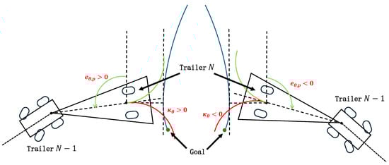
Figure 6.
Schematic of orientation tracking curvature planning. This diagram depicts two trajectories; the red curve signifies an effective reduction in orientation error, whereas the green curve fails to achieve similar results.
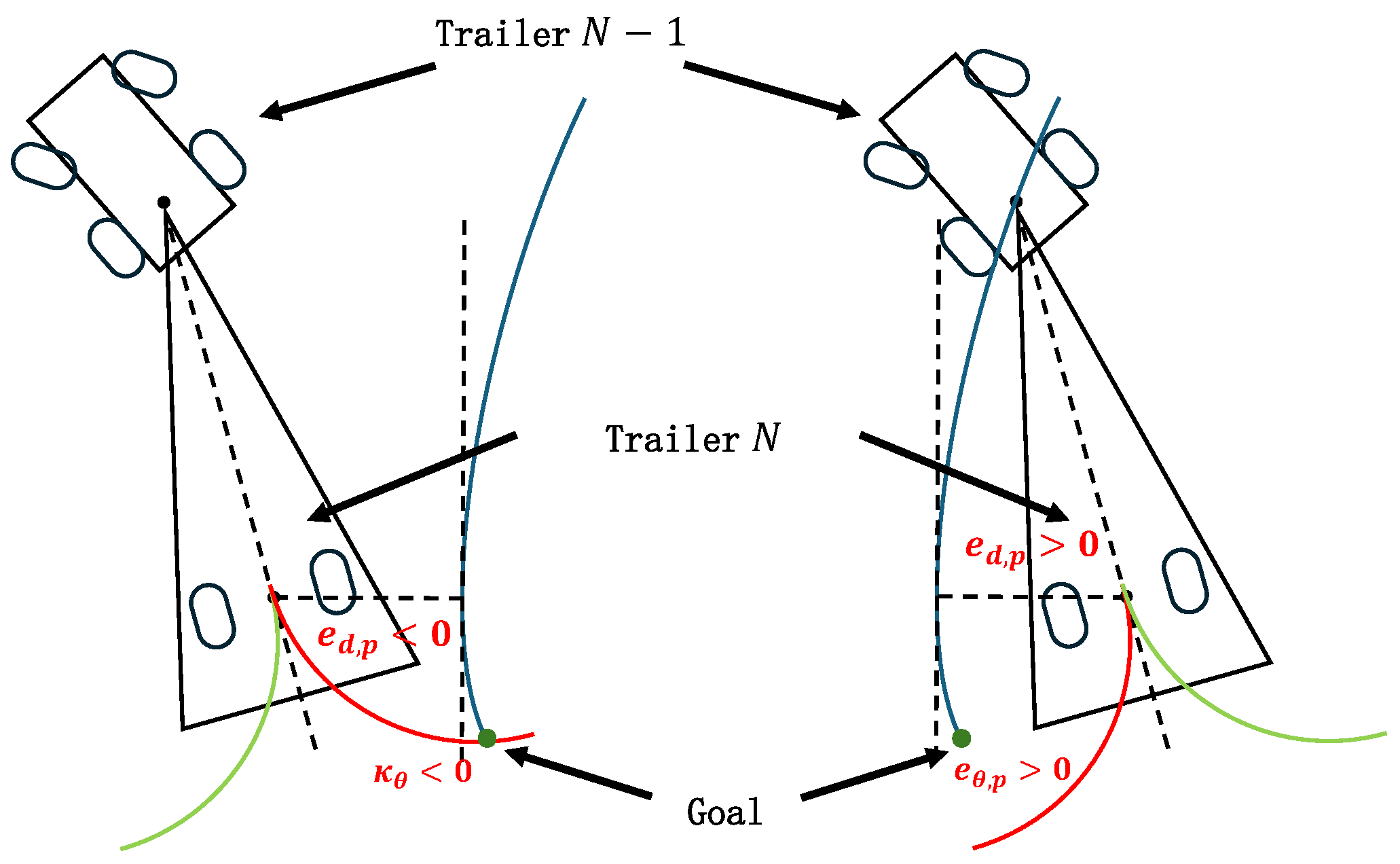
The final phase of our algorithm involves planning the distance tracking curvature, . The methodology is delineated as follows. To ensure accurate distance tracking, we establish an angular threshold such that . Distance tracking is initiated only when the magnitude of the orientation error, , is less than . As defined, the distance error signifies the lateral displacement of the tail trailer relative to a reference point p along the direction . If the tail trailer is situated to the right of point p, is positive (); conversely, if it is to the left, is negative (), as illustrated in Figure 7. When , corrective actions are taken based on the sign of . For , diminishing necessitates a clockwise reverse motion, leading to . For , the reduction in requires a counterclockwise reverse motion, resulting in . Figure 8 demonstrates the planning of the distance-tracking curvature for these scenarios, with red curves indicating the paths that effectively reduce . Therefore, the distance tracking curvature is designed as

Figure 7.
Illustration of distance error sign convention.
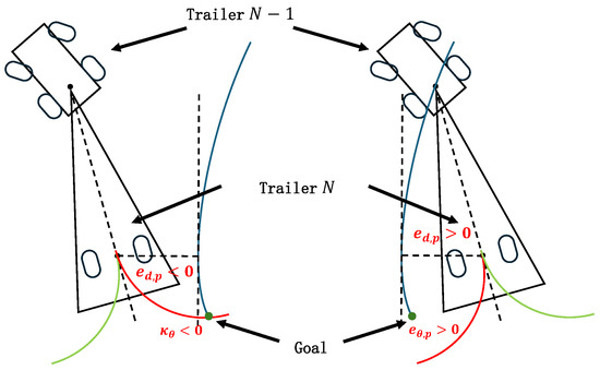
Figure 8.
Schematic of distance tracking curvature planning. This diagram depicts two trajectories; the red curve signifies an effective reduction in distance error, whereas the green curve fails to achieve similar results.
In summary, the curvature-planning result is
Remark 2
([14]). In practical applications, selecting an optimal distance tracking curvature, , that effectively addresses varying magnitudes of lateral error, , poses a significant challenge. This issue stems from the inadequacy of a linear relationship to accurately correlate the distance tracking error, , with the corresponding curvature, . A simple alternative approach is as follows:
where is the heading offset and is the heading error, which is defined in .
Using this control scheme, the control effect increases more slowly as the lateral distance error increases. In this formulation, controls the angle at which the given lateral distance error approaches the desired path. The gains determine the aggressiveness of the turns when correcting the orientation error.
3.3. Traction Velocity Determination
Section 3.1 and Section 3.2 describe the steering controls for scenarios where the traction velocity is negative. However, the specific value of has not been established. Determining an appropriate value for could significantly enhance the path-following performance of the truck-trailer system. In cases where the truck-trailer’s configuration is near the desired path, it is logical to operate at maximum velocity . In contrast, when the configuration deviates significantly from the target path, a reduction in the traction velocity is advisable. This allows for more precise adjustments in steering to realign with the desired path. For the backword motion with reference on the tail trailer, the traction velocity is set as
where is the -norm function of ·, and .
In our paper, we address three types of constraints for the truck-trailer system: nonholonomic constraints, state constraints (joint angle constraints), and input constraints. The nonholonomic constraints are governed by the system equations presented in (1). State constraints are detailed in Assumption 1, and input constraints are managed through the traction velocity determination method outlined in this section to ensure compliance.
We recognize the limitations of our control scheme, especially its potential performance degradation under complex real-world conditions. To mitigate issues arising from challenges such as road unevenness and adverse weather conditions, we plan to optimize our control strategy in future research efforts. This will enhance the robustness and applicability of our approach in varied operational environments.
4. Results
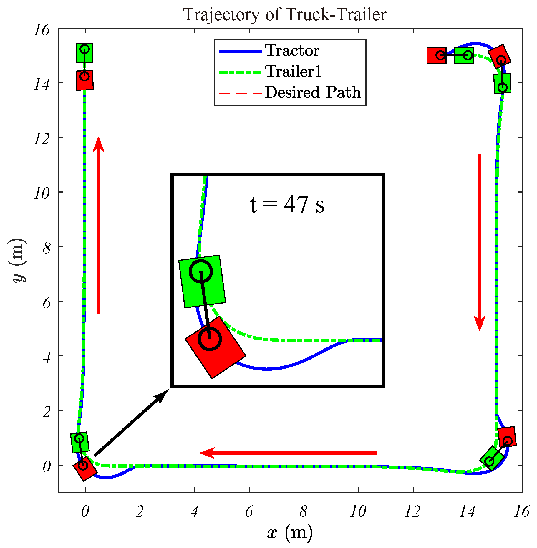
In this subsection, we evaluate the performance of the path-following control law. The maximum velocity is restricted to m/s due to the limitations of the truck-trailer prototype. The trajectory under consideration is a “U”-shaped right-angle path, as detailed in [10].
4.1. Mobile Robot with One Trailer
Simulations are conducted for a mobile robot with one trailer. Figure 9 illustrates the simulated trajectories of the truck-trailer. The path includes three segments:
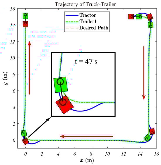
Figure 9.
Traces of the mobile robot with 1 trailer.
- Segment I: A vertical line defined by and rad.
- Segment II: A horizontal line defined by with rad.
- Segment III: Another vertical line defined by with rad.
The kinematic model parameters in (1) are m, and m. Control gains are set as , , and . The initial state of the robot is
The control input is determined through formal differentiation of , while is estimated through filtered numerical differentiation in the simulations. The results displayed in Figure 9 show the trajectories of the tractor (red block) and trailer (green block), highlighting the system’s stable reversal while tracking the path.
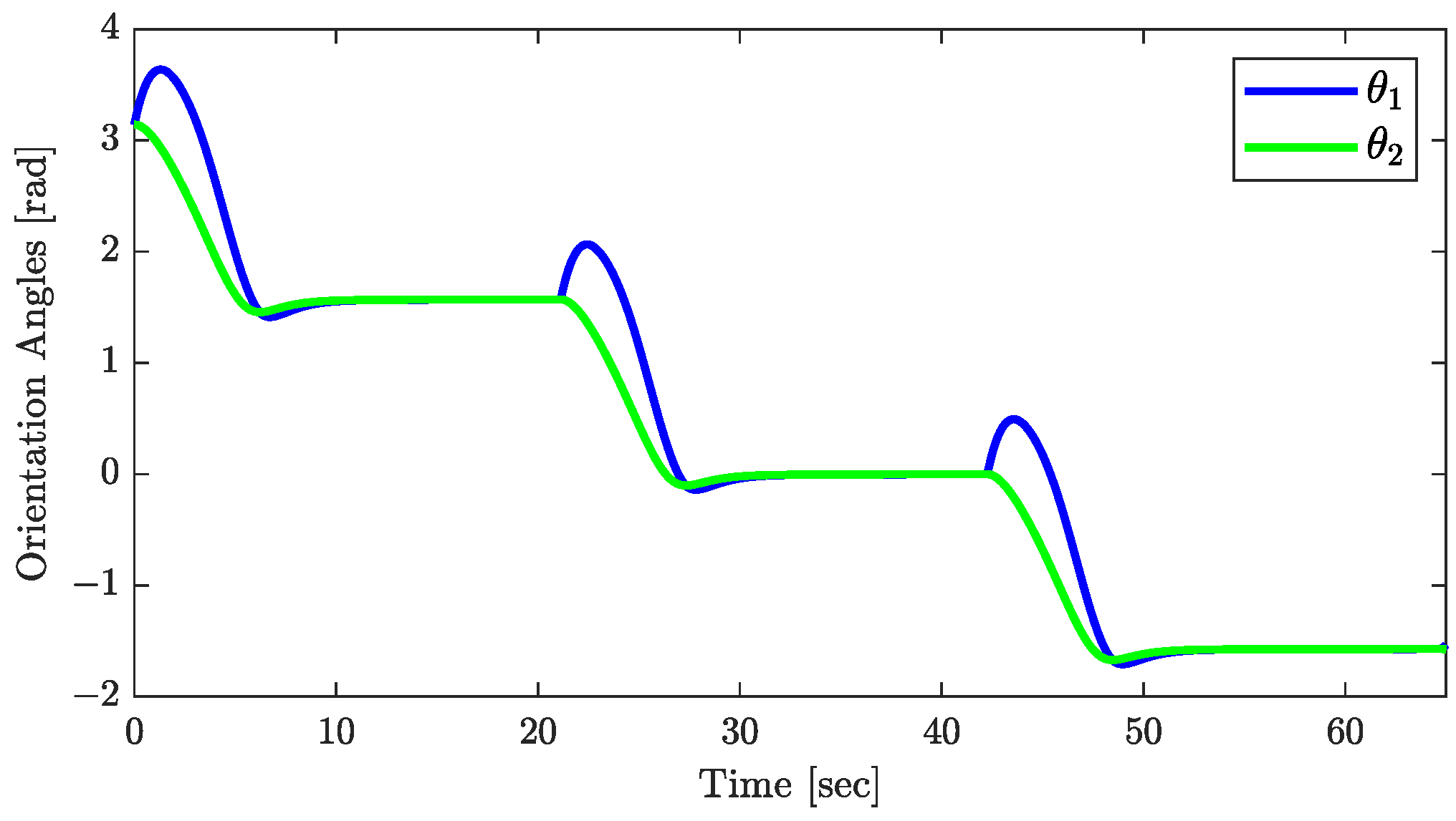
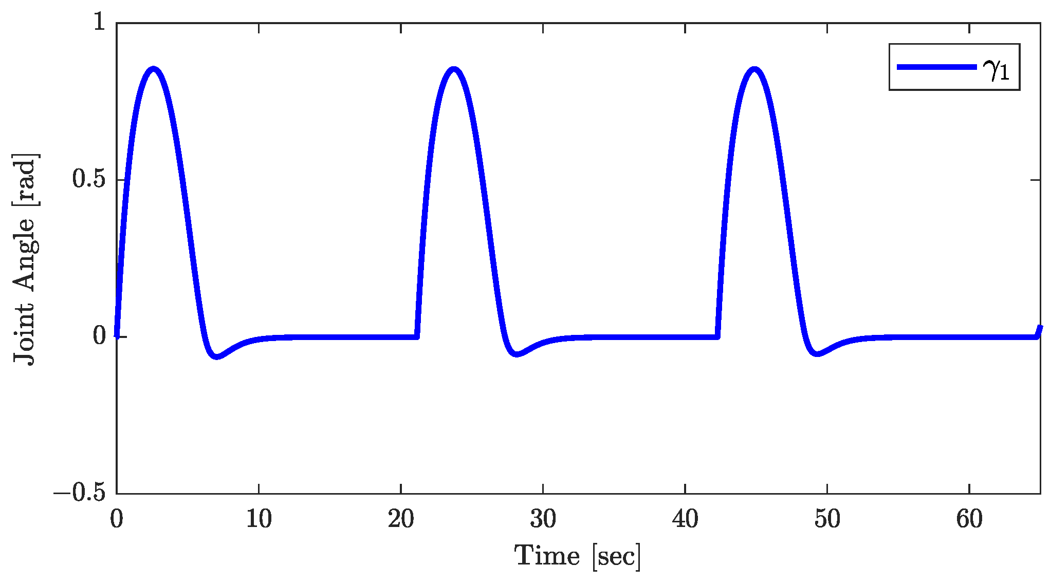
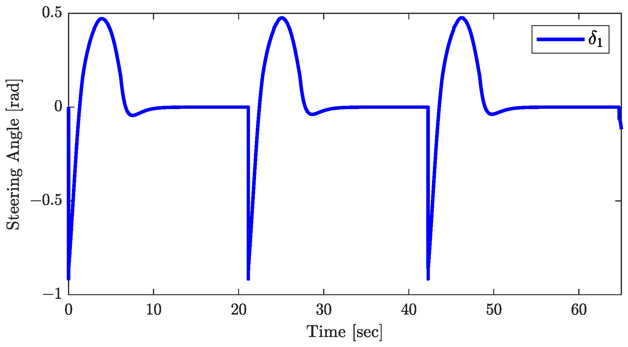
The conclusions of Theorem 1 are supported by the results in Figure 10, Figure 11 and Figure 12. Figure 10 demonstrates the asymptotic convergence of the trailer’s orientation to . The joint angle’s response, shown in Figure 11, and the control input , in Figure 12, both converge asymptotically to zero, validating the assumptions that and throughout the control process. Additionally, the responses of , plotted in Figure 13, showing that tends to zero asymptotically, are consistent with the conclusion of Theorem 1.

Figure 10.
Responses of the orientations.
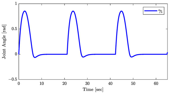
Figure 11.
Response of the joint angle.
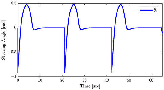
Figure 12.
Response of the control input.
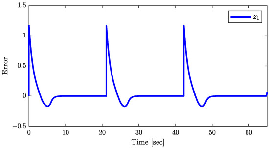
Figure 13.
Response of .
4.2. Mobile Robot with Three Trailers
Simulations are conducted for a mobile robot with three trailers. Figure 14 illustrates the simulated trajectories of the truck-trailer. The path includes three segments:
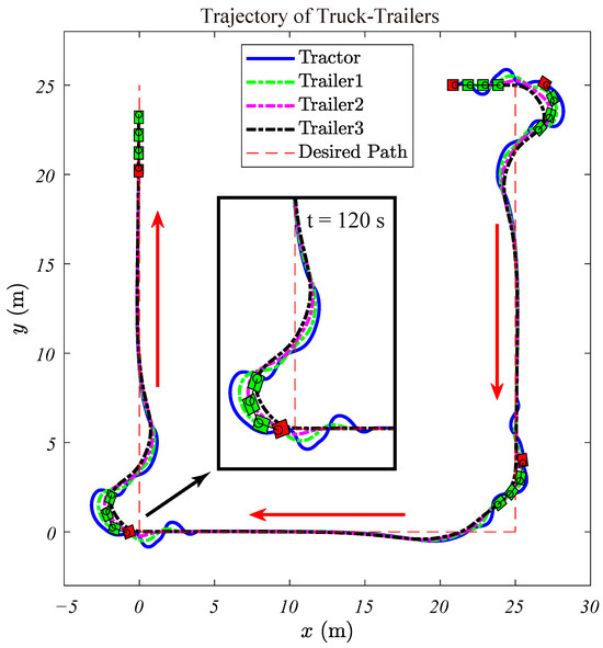
Figure 14.
Traces of the mobile robot with 3 trailers.
- Segment I: A vertical line defined by and rad.
- Segment II: A horizontal line defined by with rad.
- Segment III: Another vertical line defined by with rad.
The kinematic model parameters in (1) are m and m. Control gains are set as , , , , and . The initial state of the robot is given as
The control input is recursively calculated through the formal differentiation of . As the number of trailers increases, deriving becomes increasingly complex. Therefore, in numerical simulations, is estimated through filtered numerical differentiation.
Figure 14 displays the traces of the tractor and the three trailers. The tractor is marked with a red block, and the trailers are marked with green blocks. The assembly reverses stably while maintaining the desired orientation angle.
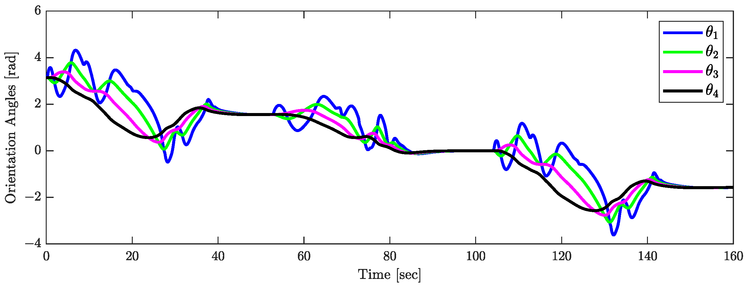
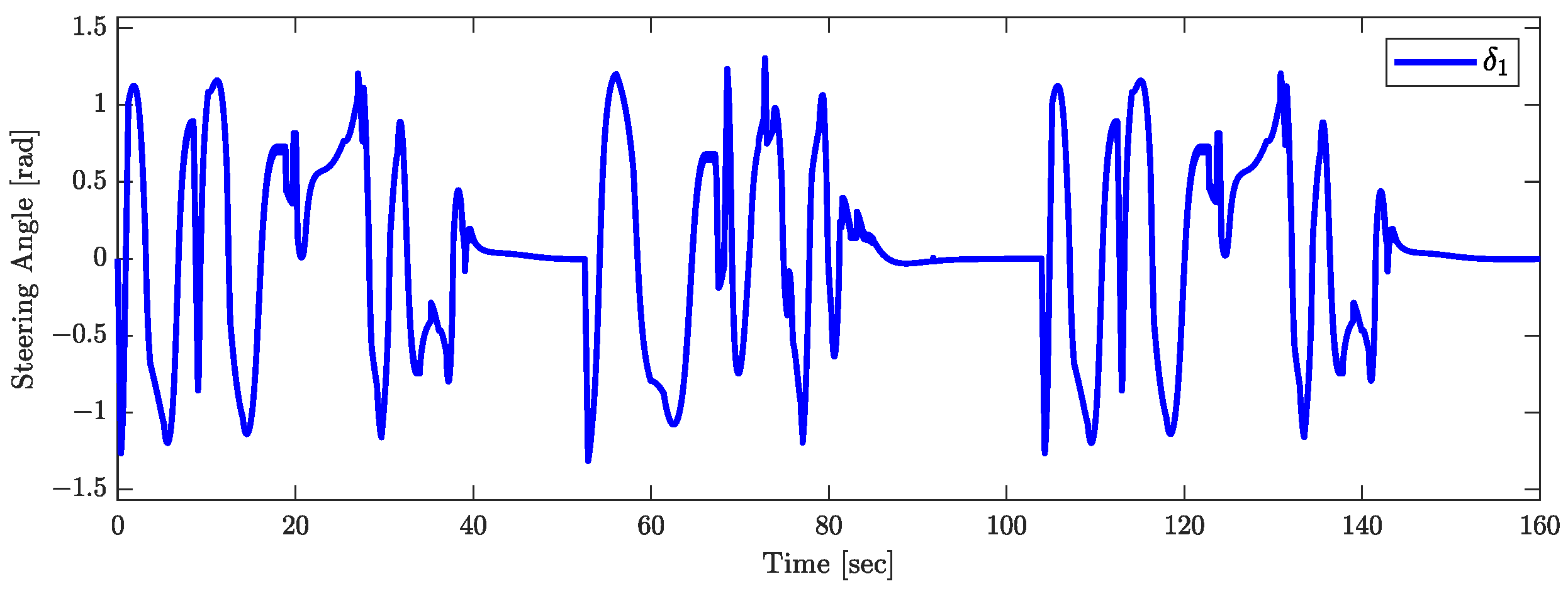
The validity of Theorem 1 is demonstrated by the results shown in Figure 15, Figure 16 and Figure 17. Figure 15 indicates that the orientations of the trailers converge asymptotically to . The joint angle responses depicted in Figure 16 support the assumption that (). Figure 17 presents the response of the control input , confirming the assumptions that . Figure 18 plots the responses of (), which tend to zero asymptotically, which is consistent with the conclusions of Theorem 1.
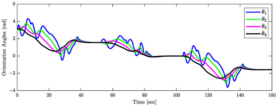
Figure 15.
Responses of the orientations.
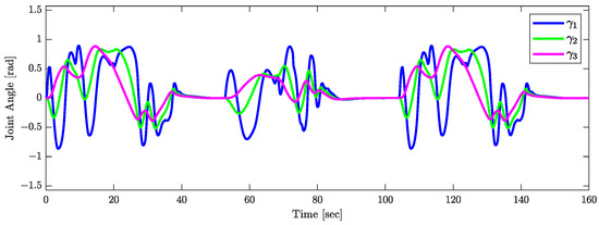
Figure 16.
Responses of the joint angles.
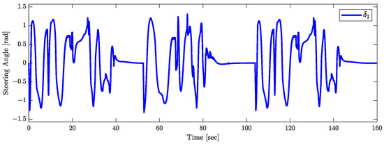
Figure 17.
Response of the control input.
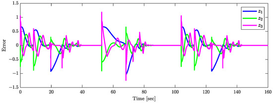
Figure 18.
Responses of .
4.3. Simulation of Curve-Path Backward-Following Control
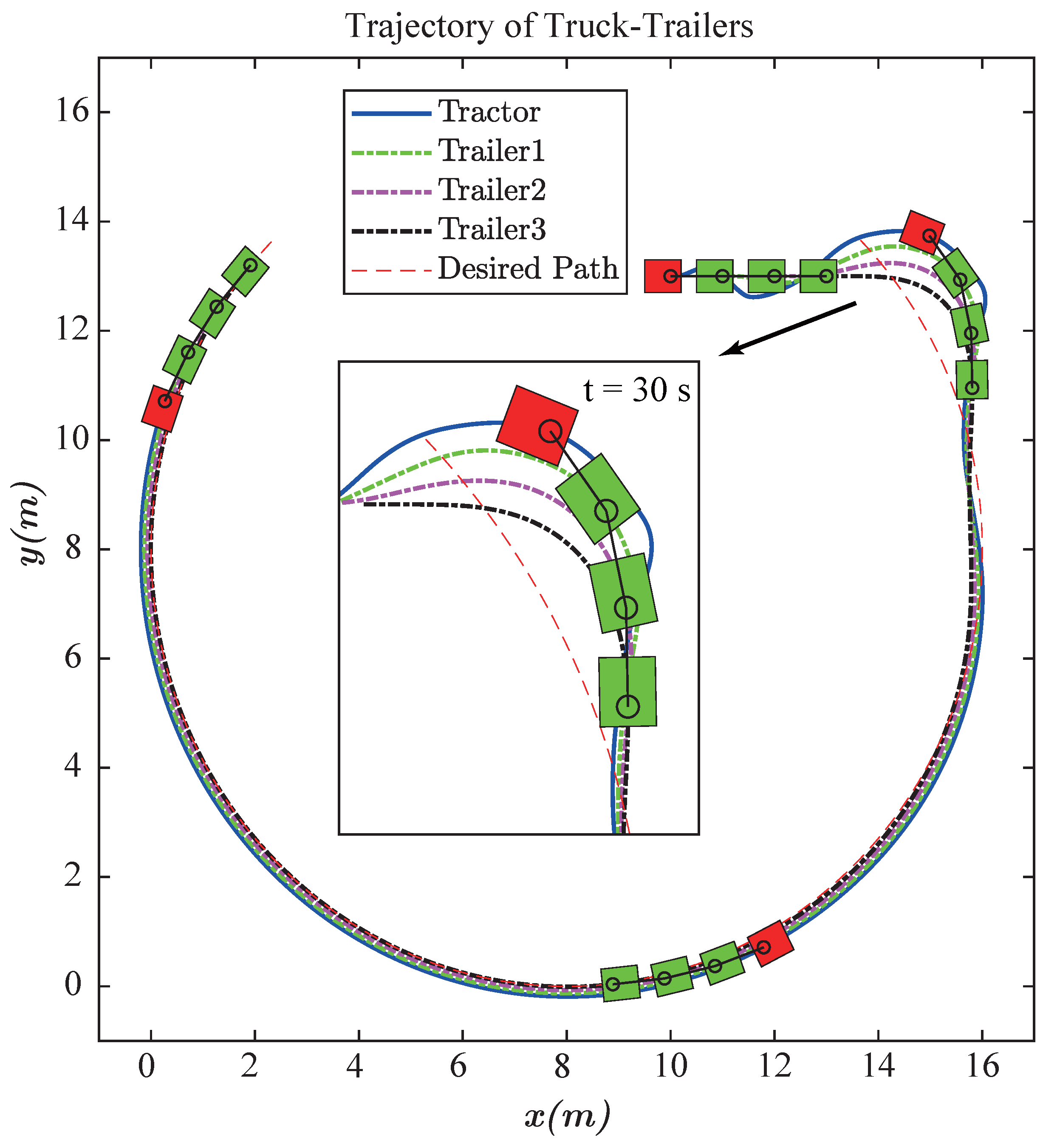
Simulations are conducted to assess the curve-path backward-following control of a truck-trailer system. The circle–curve path followed in the simulations is defined by the equation , where represents the center and r denotes the radius of the path.
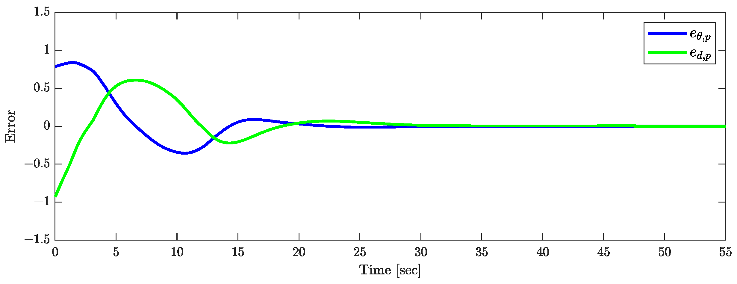
Figure 19 displays the traces of the tractor and the three trailers. Figure 20 presents the response of the tracking errors. The tail trailer follows a circle–curve path centered at with a radius of . From these figures, it is evident that starting from an initial position inside the circle, the truck-trailer is capable of accurately following the circle–curve path. The control parameters used in the simulation are consistent with those in Section 4.2.

Figure 19.
Traces of circle–curve path following.
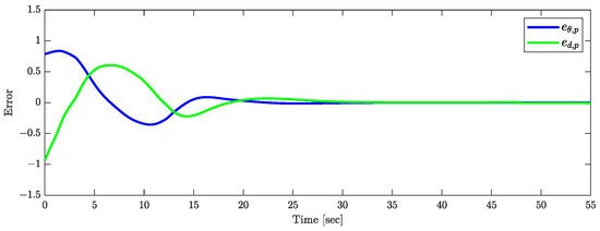
Figure 20.
Directional error and distance error .
5. Discussion
The major differences between our study and the existing literature are outlined below:
- Path Tracking for N Trailers: This research specifically tackles the path-tracking control problem for mobile robots with N trailers, which is an area that remains largely unexplored in the current literature. While prior research has dealt with configurations involving fewer trailers, our study extends these methodologies to more complex systems with N trailers, thereby pioneering and filling a gap in this field.
- Recursive Feedback Controller Design: Although inspired by the techniques outlined in [22], our controller design introduces operational changes. The error function in our controller, expressed as , contrasts with the format used in Reference [1]. This modification simplifies the computational demands and enhances control performance, making our approach both innovative and practically efficient.
- Innovative Curvature-Planning Algorithm: We have developed a novel curvature-planning algorithm specifically designed for path tracking in systems with N trailers. This algorithm does not require the tracked path to be continuously differentiable, which significantly enhances the path-tracking capabilities of mobile robots.
The limitations of our control scheme are further outlined below:
- Environmental and Terrain Influences: While we have implemented essential constraints in our control algorithm for the truck-trailer system, its performance could deteriorate under complex conditions such as varying weather or uneven terrain. These factors can disrupt the kinetic and dynamic responses of the system, presenting challenges not currently addressed by our framework.
- Stability and Optimization: The stability of our control scheme was validated using Input-to-State Stability (ISS) theory, demonstrating its exponential stability. However, we did not optimize the design and tuning of the controller beyond this validation, which limits its robustness and efficiency under varying operational conditions.
- Decoupling of Kinematic and Dynamic Controls: Our strategy requires a decoupling of kinematic and dynamic controls, necessitating operation conditions where the kinematic system operates at a lower frequency than the dynamic system. However, this requirement may restrict the responsiveness and adaptability of the control system to rapid changes in dynamics or external disturbances.
- Experimental Validation: Although previous studies have validated the curvature-based controller for mobile systems with a single trailer [9,14,15], its application to N-trailer systems is introduced for the first time in this paper. Additionally, controllers developed through the recursive design approach are inherently complex. While this paper has demonstrated the effectiveness of this approach using ISS stability theory and simulations, further experimental validation is necessary to confirm its real-world performance.
6. Conclusions
This paper presents a novel backward path-following controller for a mobile robot with N trailers. The controller comprises two layers: an outer curvature-planning algorithm and an inner curvature-tracking lateral controller. The outer layer calculates the desired curvature for the tail trailer, transforming the backward path-following problem into a curvature tracking problem. The inner layer is designed to ensure exponential convergence of the tail trailer to the desired curvature. The stability of the proposed control system is established using Lyapunov theory, and its effectiveness is corroborated by numerical simulations. Future work will concentrate on refining the existing control scheme through optimization and incorporating sensing technologies into the current framework.
Author Contributions
Conceptualization, W.Z. and Y.Z.; methodology, T.Z. and P.L.; software, P.X.; validation, T.Z., W.H. and P.X.; investigation, W.H.; writing—original draft preparation, T.Z.; visualization, T.Z. and P.X.; writing—review and editing, T.Z., W.H. and P.L. All authors have read and agreed to the published version of the manuscript.
Funding
This work is supported by a grant from the National Natural Science Foundation of China (Project Number U2033208).
Institutional Review Board Statement
Not applicable.
Informed Consent Statement
Not applicable.
Data Availability Statement
The data presented in this study are available on request from the corresponding author.
Conflicts of Interest
The authors declare no conflict of interest.
Abbreviations
The following abbreviations are used in this manuscript:
| RH | Reference head-truck |
| RT | Reference trailer |
| MPC | Model predictive controller |
| PID | Proportional–Integral–Derivative |
Appendix A
Definition A1
([22]). A continuous function is classified as belonging to class if it is strictly increasing and . It belongs to class if and as .
Definition A2
([22]). A continuous function belongs to class if, for each fixed t, the function is in class with respect to x and, for each fixed x, decreases with respect to t and approaches zero as .
References
- David, J.; Manivannan, P.V. Control of truck-trailer mobile robots: A survey. Intell. Serv. Robot. 2014, 7, 245–258. [Google Scholar] [CrossRef]
- Martinez, J.L.; Morales, J.; Mandow, A.; Garcia-Cerezo, A. Steering Limitations for a Vehicle Pulling Passive Trailers. IEEE Trans. Control. Syst. Technol. 2008, 16, 809–818. [Google Scholar] [CrossRef]
- Khalaji, A.K.; Moosavian, S.A.A. Dynamic modeling and tracking control of a car with n n trailers. Multibody Syst. Dyn. 2016, 37, 211–225. [Google Scholar]
- Khalaji, A.K.; Moosavian, S.A.A. Robust forward\backward control of wheeled mobile robots. ISA Trans. 2021, 115, 32–45. [Google Scholar] [CrossRef]
- Khalaji, A.K.; A Moosavian, S.A. Adaptive sliding mode control of a wheeled mobile robot towing a trailer. Proc. Inst. Mech. Eng. Part I: J. Syst. Control. Eng. 2015, 229, 169–183. [Google Scholar] [CrossRef]
- Kassaeiyan, P.; Tarvirdizadeh, B.; Alipour, K. Control of tractor-trailer wheeled robots considering self-collision effect and actuator saturation limitations. Mech. Syst. Signal Process. 2019, 127, 388–411. [Google Scholar] [CrossRef]
- Bin Salamah, Y. Sliding Mode Controller for Autonomous Tractor-Trailer Vehicle Reverse Path Tracking. Appl. Sci. 2023, 13, 11998. [Google Scholar] [CrossRef]
- Zhao, H.; Zhou, S.; Chen, W.; Miao, Z.; Liu, Y.H. Modeling and motion control of industrial tractor–trailers vehicles using force compensation. IEEE/ASME Trans. Mechatron. 2021, 26, 645–656. [Google Scholar] [CrossRef]
- Leng, Z.; Minor, M.A. Curvature-Based Ground Vehicle Control of Trailer Path Following Considering Sideslip and Limited Steering Actuation. IEEE Trans. Intell. Transp. Syst. 2016, 18, 332–348. [Google Scholar] [CrossRef]
- Widyotriatmo, A.; Nazaruddin, Y.Y.; Putranto, M.R.F.; Ardhi, R. Forward and backward motions path following controls of a truck-trailer with references on the head-truck and on the trailer. ISA Trans. 2020, 105, 349–366. [Google Scholar] [CrossRef]
- Kassaeiyan, P.; Alipour, K.; Tarvirdizadeh, B. A full-state trajectory tracking controller for tractor-trailer wheeled mobile robots. Mech. Mach. Theory 2020, 150, 103872. [Google Scholar] [CrossRef]
- Shojaei, K.; Abdolmaleki, M. Output feedback control of a tractor with N-trailer with a guaranteed performance. Mech. Syst. Signal Process. 2020, 142, 106746. [Google Scholar] [CrossRef]
- Yuan, J.; Sun, F.; Huang, Y. Trajectory generation and tracking control for double-steering tractor–trailer mobile robots with on-axle hitching. IEEE Trans. Ind. Electron. 2015, 62, 7665–7677. [Google Scholar] [CrossRef]
- Leng, Z.; Minor, M. A simple tractor-trailer backing control law for path following. In Proceedings of the 2010 IEEE/RSJ International Conference on Intelligent Robots and Systems, Taipei, Taiwan, 18–22 October 2010; IEEE: Piscataway, NJ, USA, 2010; pp. 5538–5542. [Google Scholar]
- Leng, Z.; Minor, M.A. A simple tractor-trailer backing control law for path following with side-slope compensation. In Proceedings of the 2011 IEEE International Conference on Robotics and Automation, Shanghai, China, 9–13 May 2011; IEEE: Piscataway, NJ, USA, 2011; pp. 2386–2391. [Google Scholar]
- Crenganiș, M.; Breaz, R.-E.; Racz, S.-G.; Gîrjob, C.-E.; Biriș, C.-M.; Maroșan, A.; Bârsan, A. Fuzzy Logic-Based Driving Decision for an Omnidirectional Mobile Robot Using a Simulink Dynamic Model. Appl. Sci. 2024, 14, 3058. [Google Scholar] [CrossRef]
- Robat, A.B.; Arezoo, K.; Alipour, K.; Tarvirdizadeh, B. Dynamics modeling and path following controller of tractor-trailer-wheeled robots considering wheels slip. ISA Trans. 2024, 148, 45–63. [Google Scholar] [CrossRef]
- Latif, A.; Chalhoub, N.; Pilipchuk, V. Control of the nonlinear dynamics of a truck and trailer combination. Nonlinear Dyn. 2020, 99, 2505–2526. [Google Scholar] [CrossRef]
- Oriolo, G.; De Luca, A.; Vendittelli, M. WMR control via dynamic feedback linearization: Design, implementation, and experimental validation. IEEE Trans. Control. Syst. Technol. 2002, 10, 835–852. [Google Scholar] [CrossRef]
- Widyotriatmo, A.; Hong, K.-S. Switching algorithm for robust configuration control of a wheeled vehicle. Control Eng. Pract. 2012, 20, 315–325. [Google Scholar] [CrossRef]
- Cheng, J.; Zhang, Y.; Wang, Z.; Gong, L. Backward Circular Motion Control for Mobile Robot with Two Trailers. In Proceedings of 2013 Chinese Intelligent Automation Conference: Intelligent Automation; Springer: Berlin/Heidelberg, Germany, 2013; pp. 145–151. [Google Scholar]
- Cheng, J.; Wang, B.; Zhang, Y.; Wang, Z. Backward orientation tracking control of mobile robot with N trailers. Int. J. Control Autom. Syst. 2017, 15, 867–874. [Google Scholar] [CrossRef]
- Cheng, J.; Wang, B.; Xu, Y. Backward path tracking control for mobile robot with three trailers. In Proceedings of the Neural Information Processing: 24th International Conference, ICONIP 2017, Guangzhou, China, 14–18 November 2017; Part VI 24. Springer International Publishing: Berlin/Heidelberg, Germany; pp. 32–41. [Google Scholar]
- Bai, G.; Meng, Y.; Liu, L.; Luo, W.; Gu, Q.; Li, K. A New Path Tracking Method Based on Multilayer Model Predictive Control. Appl. Sci. 2019, 9, 2649. [Google Scholar] [CrossRef]
- Shojaei, K. Neural network formation control of a team of tractor–trailer systems. Robotica 2018, 36, 39–56. [Google Scholar] [CrossRef]
- Zhao, Y. Robust Predictive Control of Input Constraints and Interference Suppression for Semi-Trailer System. Int. J. Control Autom. 2014, 7, 371–382. [Google Scholar] [CrossRef]
- Xu, P.; Cui, Y.; Shen, Y.; Zhu, W.; Zhang, Y.; Wang, B.; Tang, Q. Reinforcement learning compensated coordination control of multiple mobile manipulators for tight cooperation. Eng. Appl. Artif. Intell. 2023, 123, 106281. [Google Scholar] [CrossRef]
- Michałek, M.M.; Pazderski, D. Forward tracking of complex trajectories with non-Standard N-Trailers of non-minimum-phase kinematics avoiding a jackknife effect. Int. J. Control 2019, 92, 2547–2560. [Google Scholar] [CrossRef]
- Sanders, D.A. Non-Model-Based Control of a Wheeled Vehicle Pulling Two Trailers to Provide Early Powered Mobility and Driving Experiences. IEEE Trans. Neural Syst. Rehabil. Eng. 2017, 26, 96–104. [Google Scholar] [CrossRef]
- Yue, M.; Hou, X.; Gao, R.; Chen, J. Trajectory tracking control for tractor-trailer vehicles: A coordinated control approach. Nonlinear Dyn. 2018, 91, 1061–1074. [Google Scholar] [CrossRef]
- Manav, A.C.; Lazoglu, I.; Aydemir, E. Adaptive Path-Following Control for Autonomous Semi-Trailer Docking. IEEE Trans. Veh. Technol. 2021, 71, 69–85. [Google Scholar] [CrossRef]
- Ljungqvist, O.; Axehill, D.; Pettersson, H. On sensing-aware model predictive path-following control for a reversing general 2-trailer with a car-like tractor. In Proceedings of the 2020 IEEE International Conference on Robotics and Automation (ICRA), Paris, France, 31 May–31 August 2020; IEEE: Piscataway, NJ, USA, 2020; pp. 8813–8819. [Google Scholar]
- Jean, F. The singular locus for the n-trailers car control system. In Proceedings of the 1995 34th IEEE Conference on Decision and Control, New Orleans, LA, USA, 13–15 December 1995; IEEE: Piscataway, NJ, USA, 1995; Volume 4, pp. 3869–3870. [Google Scholar]
- Haddad, W.M.; Chellaboina, V. Nonlinear Dynamical Systems and Control: A Lyapunov-Based Approach; Princeton University Press: Princeton, NJ, USA, 2008. [Google Scholar]


Disclaimer/Publisher’s Note: The statements, opinions and data contained in all publications are solely those of the individual author(s) and contributor(s) and not of MDPI and/or the editor(s). MDPI and/or the editor(s) disclaim responsibility for any injury to people or property resulting from any ideas, methods, instructions or products referred to in the content. |
© 2024 by the authors. Licensee MDPI, Basel, Switzerland. This article is an open access article distributed under the terms and conditions of the Creative Commons Attribution (CC BY) license (https://creativecommons.org/licenses/by/4.0/).