Article

Fault Detection of Multi-Wheeled Robot Consensus Based on EKF

1
MACS Research Laboratory, Engineering School of Gabes, University of Gabes, Zrig 6029, Tunisia
2
Quartz Lab, 95014 Cergy-Pontoise, France
3
ESEO, Western Higher School of Electronics, Vélizy-Villacoublay, 78140 Paris, France
*
Author to whom correspondence should be addressed.
Actuators 2024, 13(7), 253; https://doi.org/10.3390/act13070253
Submission received: 6 May 2024 / Revised: 17 June 2024 / Accepted: 24 June 2024 / Published: 1 July 2024
(This article belongs to the Special Issue Actuators in Robotic Control: Volume II)

Abstract

:
Synchronizing a network of robots in consensus is an important task for cooperative work. Detecting faults in a network of robots in consensus is a much more important task. In considering a formation of Wheeled Mobile Robots (WMRs) in a master–slave architecture modeled by graph theory, the main objective of this study was to detect and isolate a fault that appears on a robot of this formation in order to remove it from the formation and continue the execution of the assigned task. In this context, we exploit the extended Kalman filter (EKF) to estimate the state of each robot, generate a residual, and deduce whether a fault exists. The implementation of this technique was proven using a Matlab simulator.

1. Introduction

In recent years, there has been a significant shift in focus toward cooperative multi-agent control (MAS) within the realm of control research. This shift is driven by its rapid advancement across various domains, including several robot systems, intelligent transportation, and numerous industrial setups [1,2,3,4,5]. The primary benefit of MAS lies in its ability to enhance system functionality, often overcoming challenges that may prove difficult for humans or even entirely superseding human involvement in executing tasks that are repetitive, hazardous, or beyond human capability [6]. Consequently, the importance of fault detection and isolation has escalated, ensuring safety and maintaining quality standards. Given the inevitability of faults in embedded systems such as wheeled mobile robots (WMRs), it is imperative to ensure that they are promptly identified and addressed. To facilitate and guarantee communication between robots, graph theory is used, which plays a crucial role in modeling the interactions and communication between multiple robots. In representing the robots as nodes and their communication links as edges, graph theory provides a framework for analyzing and designing consensus algorithms. This theoretical foundation is critical in ensuring that all robots in the network can agree on a common set of parameters or states, despite potential faults or communication delays.
Within computer networking, the master–slave model serves as a communication protocol wherein a designated device or process (referred to as the master) governs one or more other devices or processes (the slaves). In a master–slave relationship, the master is often the transmitter of control to the slave.
Master–slave systems often provide data security, improved consistency, and robust fault tolerance. However, their significant drawback arises in the event of master failure, which can lead to the entire system’s failure, causing process malfunctions and subsequent degradation in performance [7]. Hence, the necessity of implementing process monitoring and fault detection systems becomes paramount, especially in applications like wheeled robots. This prompts exploration into fault diagnosis techniques to effectively address this challenge. Fault detection and isolation (FDI) has garnered substantial attention in both academic and industrial spheres, as evidenced by recent publications, for example, [8]. According to [9], this methodology is typically categorized into three overarching groups: hardware redundancy methods, model-based methods, and signal analysis methods. There are two other main forks: quantitative approaches and qualitative approaches. In the literature, considerable attention has been directed toward the observer-based technique. For instance, in [10], a method utilizing Kalman filter identification was utilized for the detection and isolation of sensor faults within mobile robotic systems. Also, in [11], the authors presented the integration of a bank of Kalman filters with an expert system for the detection and isolation of sensor faults in mobile robots. Additionally, [12] introduced a Kalman filter designed for joint state prediction and unknown input estimation within linear stochastic discrete-time systems subject to intermittent unknown inputs in measurements. FDI in nonlinear systems has increased significantly in recent years because most of the systems we encounter in practice are nonlinear. For example, in [13], the FDI system is based on a single-model EKF filter that generates residuals as soon as the behavior of the aircraft deviates from the expected trajectory. Also, refs. [14,15] directed their focus toward fault detection in wheeled mobile robots utilizing an EKF filter. The fault detection process typically involves two primary steps: residual generation and subsequent residual evaluation. In our contribution, we will emphasize the observer-based approach, particularly the utilization of the extended Kalman filter.
The main contribution of this article is to detect and isolate faults in a network of robots synchronized to carry out a common task in a master–slave configuration. Robot synchronization is based on graph theory, and fault detection is implemented via the Extented Kalman Filter approach. A new procedure is established to isolate the defective robot from a formation of robots, the majority of which are affected by a defect appearing in one robot.
To present our investigation on fault detection and isolation within a nonlinear system, specifically a wheeled mobile robot, utilizing the extended Kalman filter, this paper is structured as follows. The first section outlines the modeling of a unicycle mobile robot. In the subsequent section, we delve into the extended Kalman filter (EKF) as a corrective predictor technique. This section covers two primary tasks, encompassing prediction and correction phases, alongside the fault diagnosis steps, which include residual generation, evaluation, and decision-making processes. Following this, simulations are presented to illustrate the exploitation of the EKF to detect and generate residues for a faulty master–slave system. Finally, the last section concludes the paper.

2. Multi-Wheeled Robot Consensus

In this section, we delve into the consensus algorithms for multi-wheeled robots, utilizing graph theory to model and analyze the interactions between robots. By employing graph-theoretic concepts, we can design robust consensus protocols that ensure that all robots achieve a unified state.

2.1. Graph Theory

2.1.1. Notation

We denote the set of real numbers as R . The notation R n represents the real vector space with n dimensions, while R n × n denotes the set of n × n matrices. A diagonal matrix of size n × n , with diagonal elements q 1 , q 2 , . . . , q n , is denoted as d i a g ( q 1 , q 2 , . . . , q n ) . The identity matrix is represented by I R n × n . The Kronecker product of matrices is denoted by ⊗. Additionally, we utilize x = ( x 1 , . . . , x n ) T to signify the vector in R n . The T in the exponent means transposition.

2.1.2. Graph Theory

Understanding the fundamental concepts of graph theory is indispensable for exploring the dynamics of multi-agent systems [16]. Consider a multi-agent system comprising n mobile robots interconnected through a communication network. The interaction model among agents can be represented by delineating the communication topology in the form of a graph.
Consider G t = ( Λ , Υ ) an oriented graph, where Λ = [ Λ 1 , Λ 2 , . . . , Λ n ] represents the set of nodes. Each node i represents the i t h agent, and
Υ = ( i , j ) Λ × Λ , j N i
represents the collection of edges linking the nodes, where N i denotes the set of node indexes connected to the i t h node. Here, ( i ; j ) signifies a connection between nodes i and j, with j being in N i , although i may not be in N j . Therefore, ( i ; j ) and ( j ; i ) do not obligatory denote the same edge. These node connections are consolidated into a matrix M d = [ a i j ] , known as the adjacency matrix or connection matrix, with dimensions N N . The elements within the matrix indicate whether pairs of vertices are adjacent in the graph or not.
a k j = 1 i f   k   i s   c o n n e c t e d   t o   j 0 i f   n o t .
The degree matrix Q is a diagonal matrix of size N × N , providing information regarding the number of edges connected to each node.
Q i j = d e g r e e ( Δ i ) i f   i = j 0 i f   n o t .
The Laplacian matrix H = [ l i j ] is represented by
H = Q M
The components within this matrix are as follows::
h k j = a k j i f   k j j = 1 N a k j i f   k = j .

2.1.3. Closed-Loop System

Consider a collection of N = 3 agents of significant scale, wherein the conduct of each agent is delineated by a nonlinear controlled model.
Figure 1 shows the master–slave configuration considered in this study, and the matrices are as follows:
A = 0 0 0 1 0 0 0 1 0 , D = 0 0 0 0 1 0 0 0 1 and L = 0 0 0 1 1 0 0 1 1
Remember, the protocol can be written as follows:
u i = P ( X i ) ( j = 1 N a i j ( X i X j ) )
where P ( X i ) n × m , and a i j are the adjacent elements linked to G .

2.2. Wheeled Mobile Robot Modeling

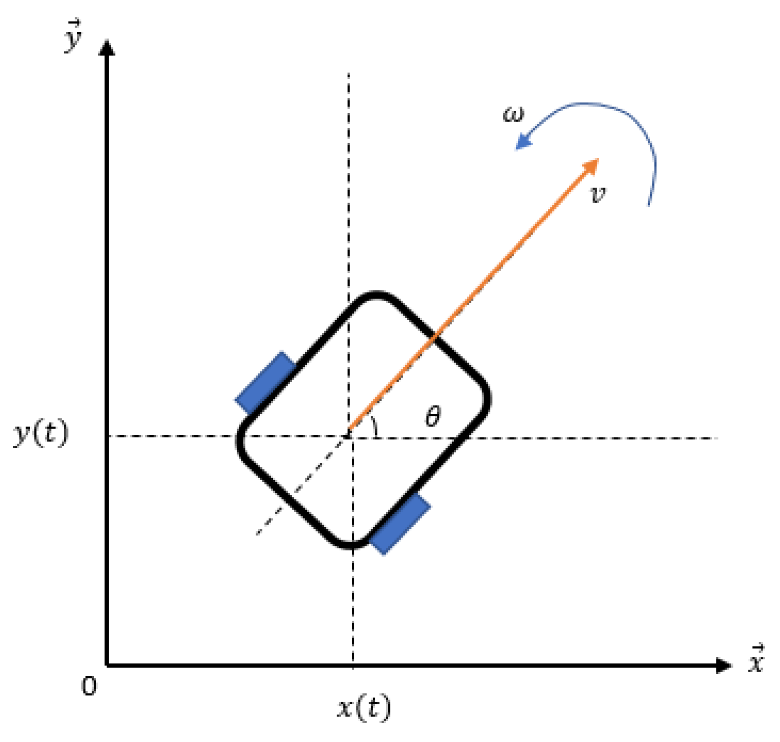
A unicycle is a robot driven by two independent wheels. It moves in a planar area referenced by an inertial reference ( 0 , x , y ) . The kinematic model is illustrated in Figure 2.
The continuous state-space representation is given as follows:
x ˙ ( t ) = v cos ( θ ( t ) ) y ˙ ( t ) = v sin ( θ ( t ) ) θ ˙ ( t ) = ω ( t ) v ˙ ( t ) = a ( t )
where x and y denote the position along the x-axis and the y-axis, respectively; v represents the linear speed associated with the center of mass; θ is the orientation angle; ω is the angular speed of the center of mass; a is the acceleration; and u represents the input vector u = ω a T . Then, the generalized robot model is given by
X ˙ ( t ) = f ( X , u , t ) Y ( t ) = C X ( t )
where X = x y θ v T is the state vector, and C = 1 0 0 0 0 1 0 0 is the observation matrix that provides the system its observability condition.
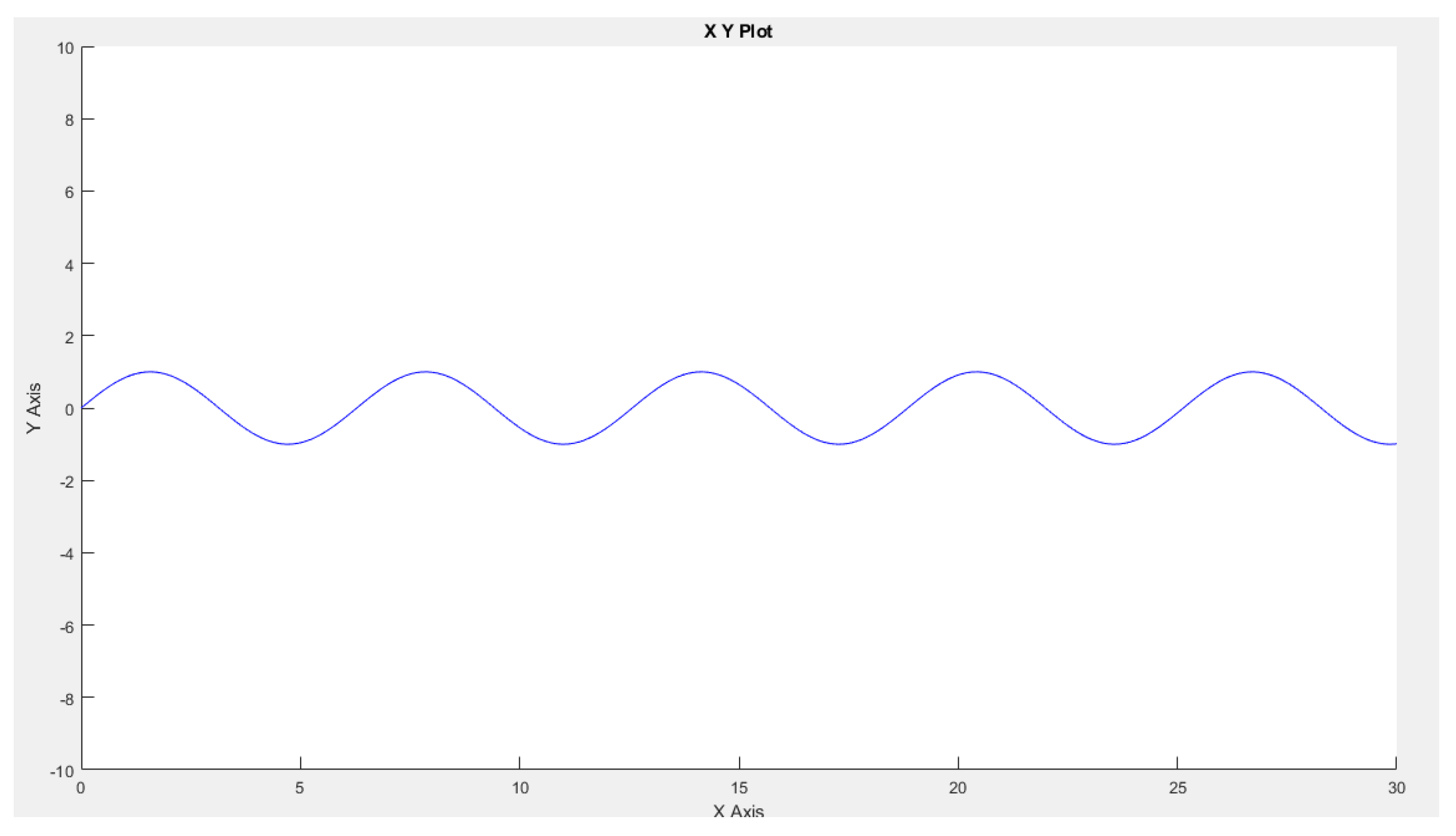
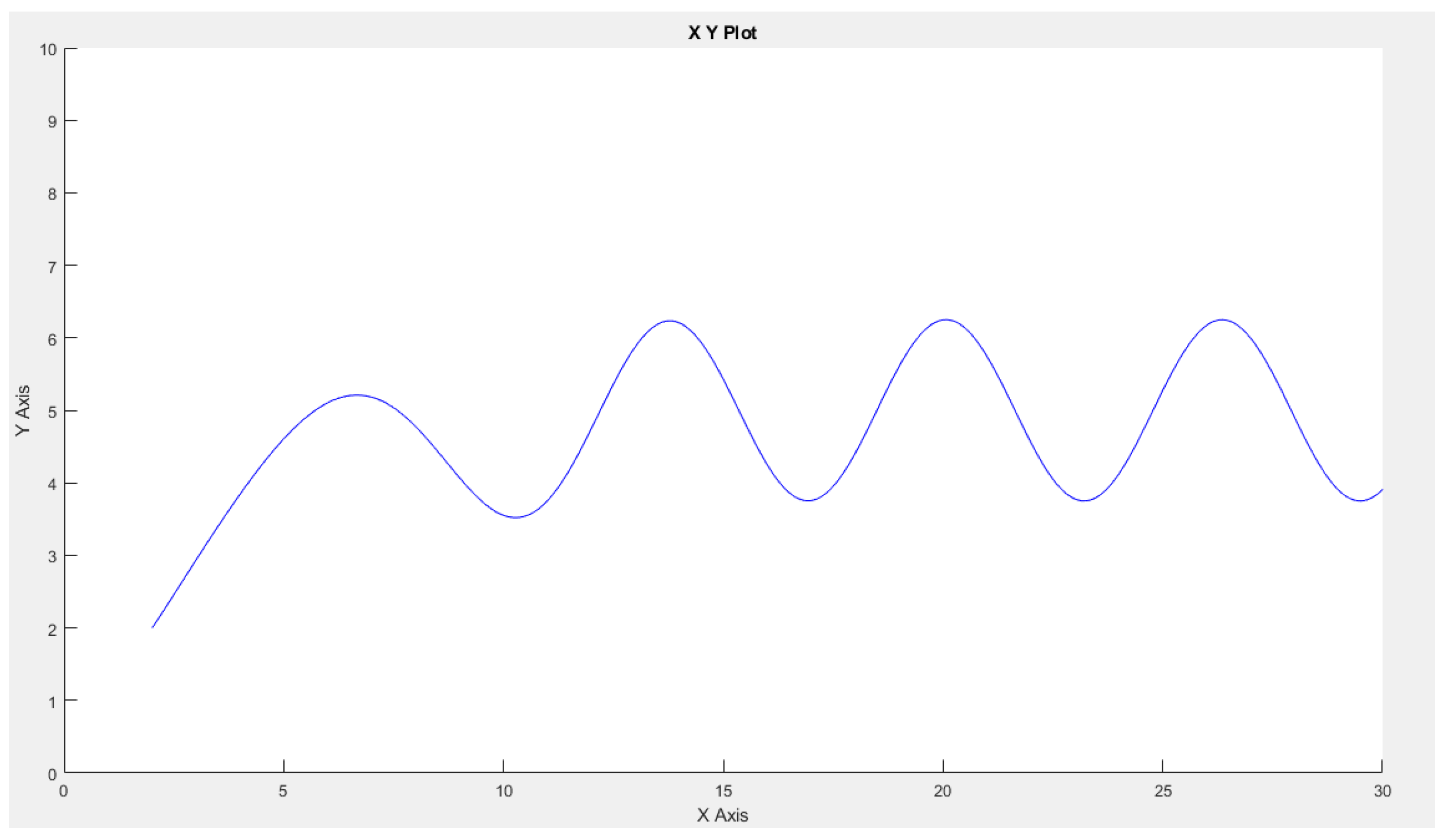
We studied a sinusoidal trajectory, so we developed a regulator that allows us to control the robot.
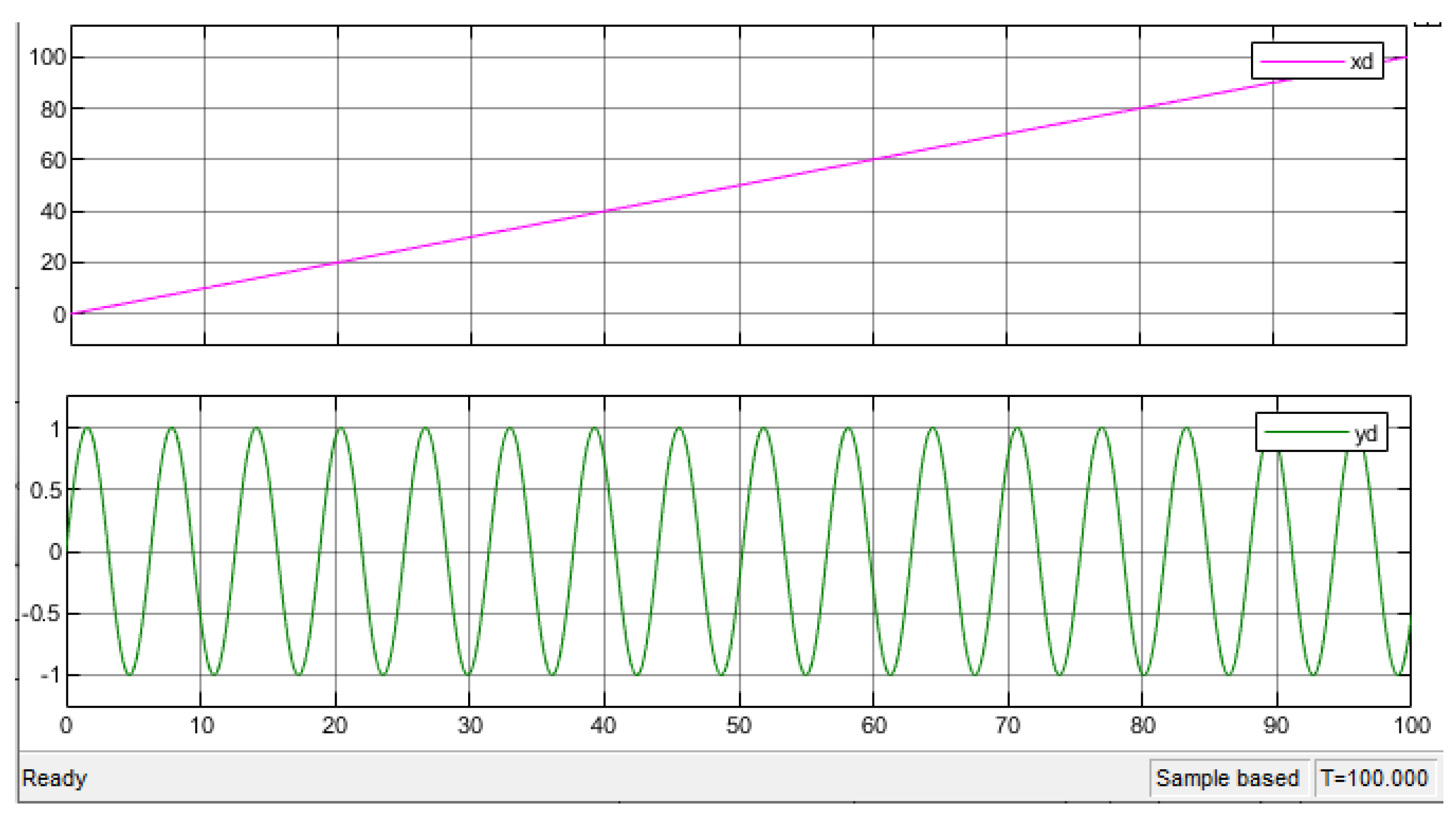
x d ( t ) = t y d ( t ) = sin ( t )
For this, we used the method of linearizing looping. The command will be, in the end, as follows:
u 1 u 2 = v sin ( θ ) cos ( θ ) v cos ( θ ) sin ( θ ) 1 ( x d x ) + 2 ( x ˙ v cos ( θ ) ) + x d ¨ ( y d y ) + 2 ( y ˙ v sin ( θ ) ) + y d ¨
If we define the error vector,
e = ( e x , e y )
the dynamics of the error are written as follows:
e x + 2 e x ˙ + e x ¨ e y + 2 e y ˙ + e y ¨ = 0 0
which is stable and converges rapidly to 0. According to Euler’s approximation, we discretize state model ( 1 ) using a sampling time T e as follows:
x k + 1 = x k + T e v k cos ( θ k ) y k + 1 = y k + T e v k sin ( θ k ) θ k + 1 = θ k + T e ω k v k + 1 = v k + T e a k

2.3. Simulations

NOTATION:
  • m: The master robot,
  • s 1 : The first slave robot,
  • s 2 : The second slave robot,
  • X d = x d y d θ d v d T : State vector of the desired trajectory,
  • X m = x m y m θ m v m T : State vector of the master robot,
  • X s 1 = x s 1 y s 2 θ s 1 v s 1 T : State vector of the first slave robot,
  • X s 2 = x s 2 y s 2 θ s 2 v s 2 T : State vector of the second slave robot,
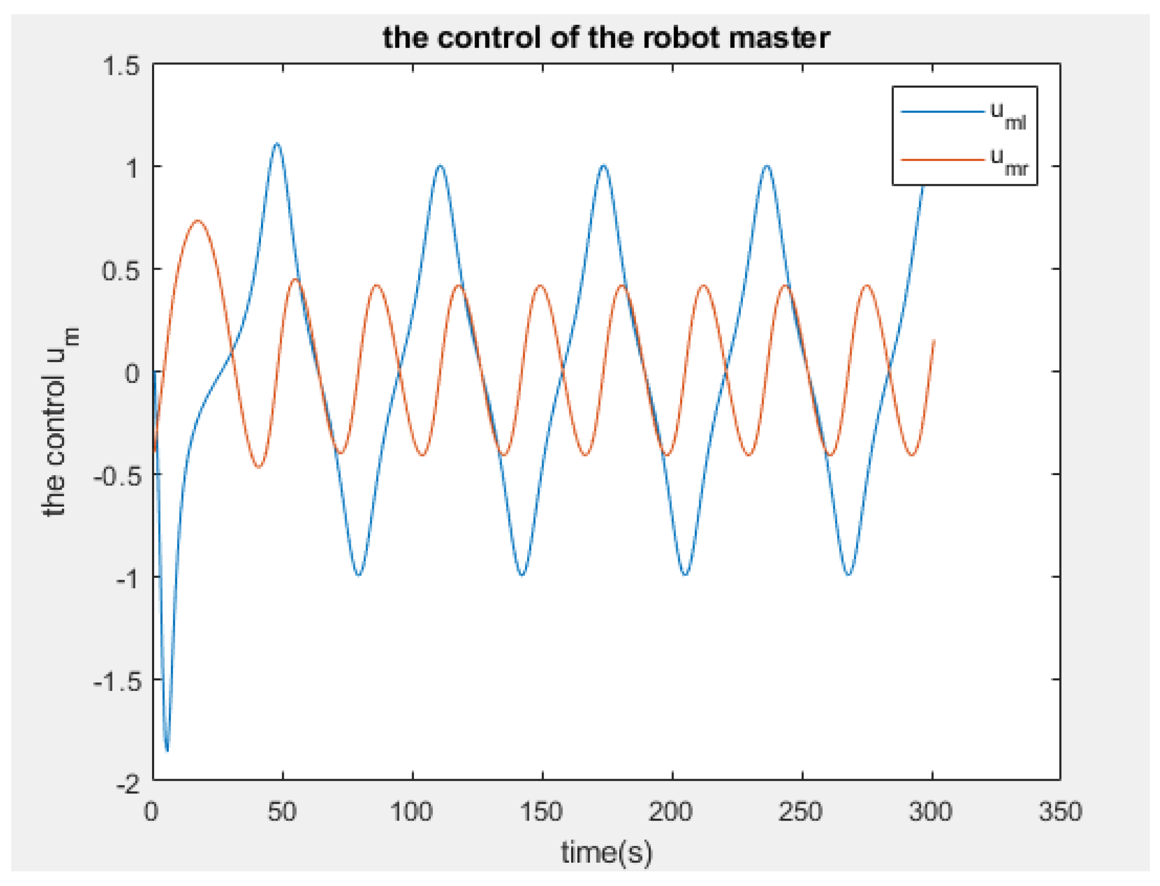
  • u m = u m l u m r T : The left and right controllers of the master robot,
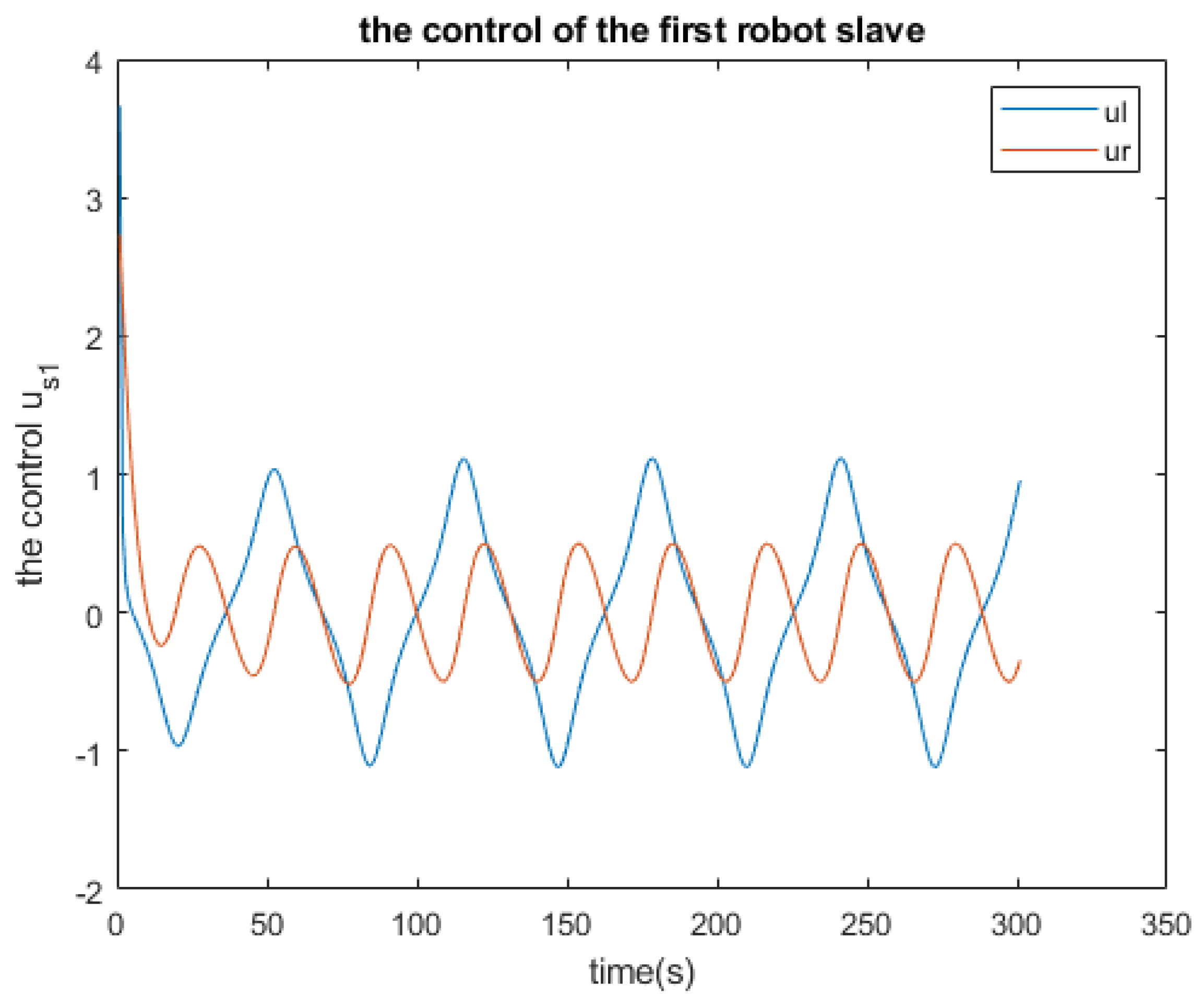
  • u s 1 = u s 1 l u s 1 r T : The left and right controllers of the first slave robot,
  • u s 2 = u s 2 l u s 2 r T : The left and right controllers of the second slave robot.
Consider the desired trajectory in Figure 3.
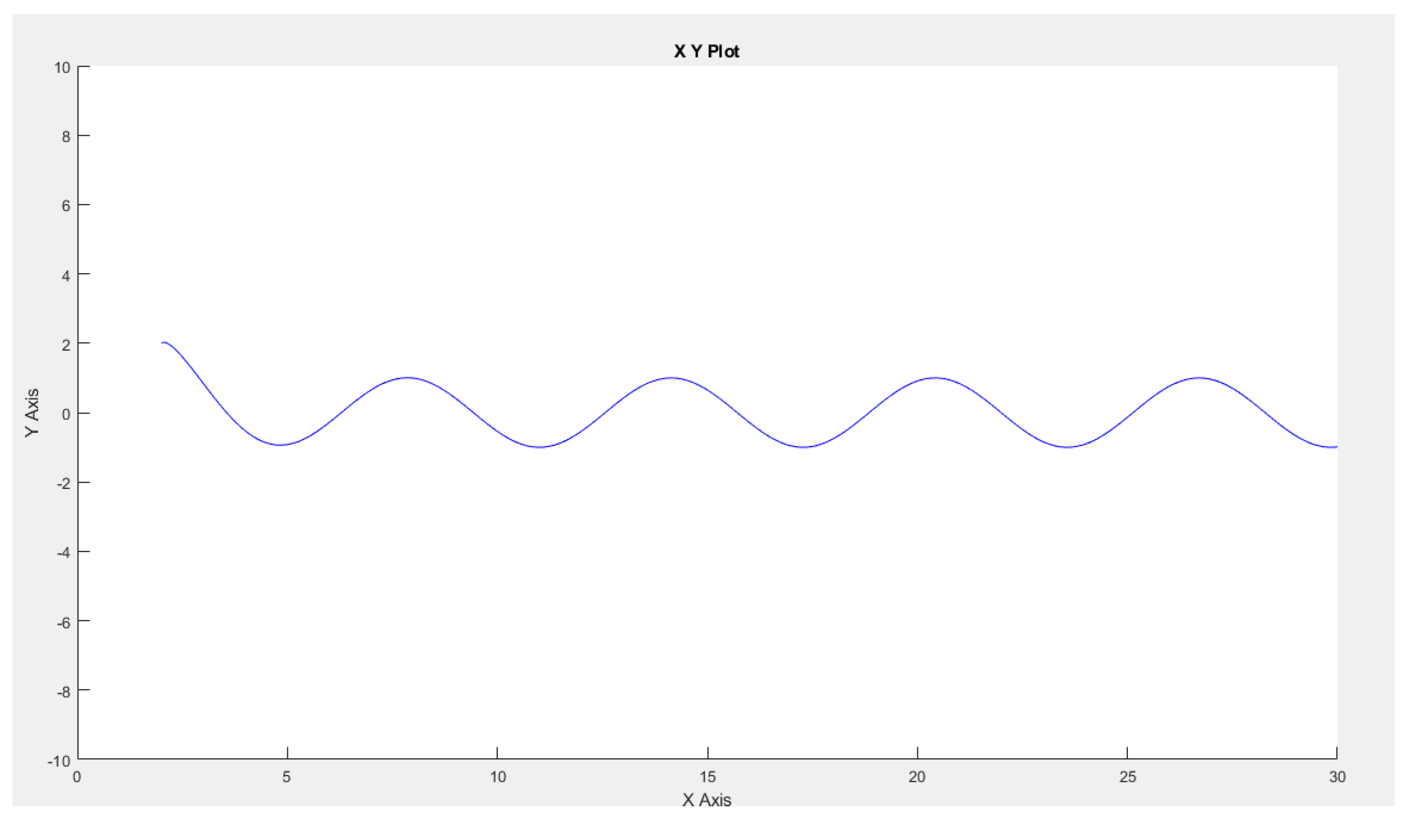
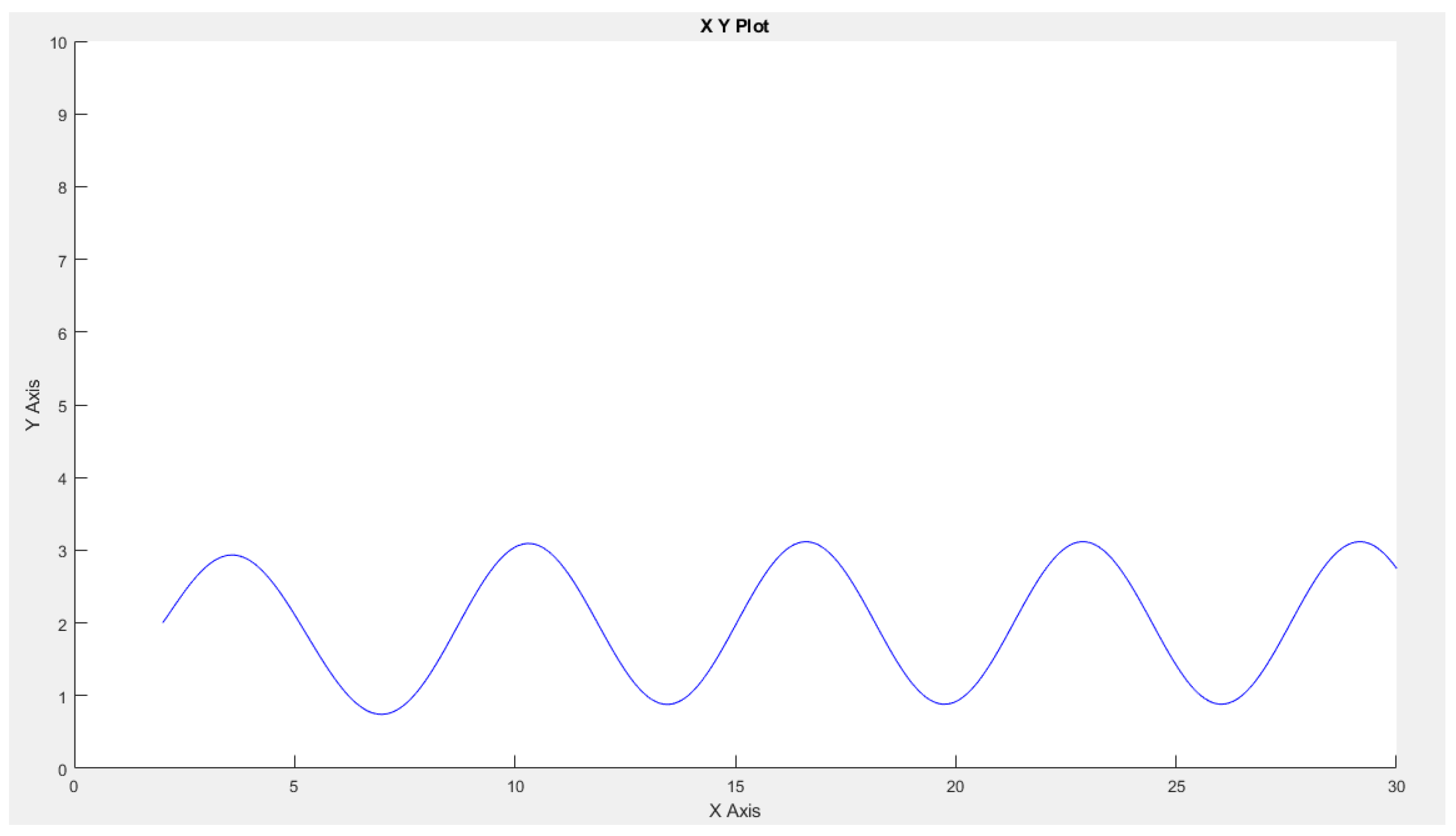
We observe that the robot master accurately follows this trajectory, which is also replicated by the two robot slaves, as depicted in Figure 4, Figure 5 and Figure 6.
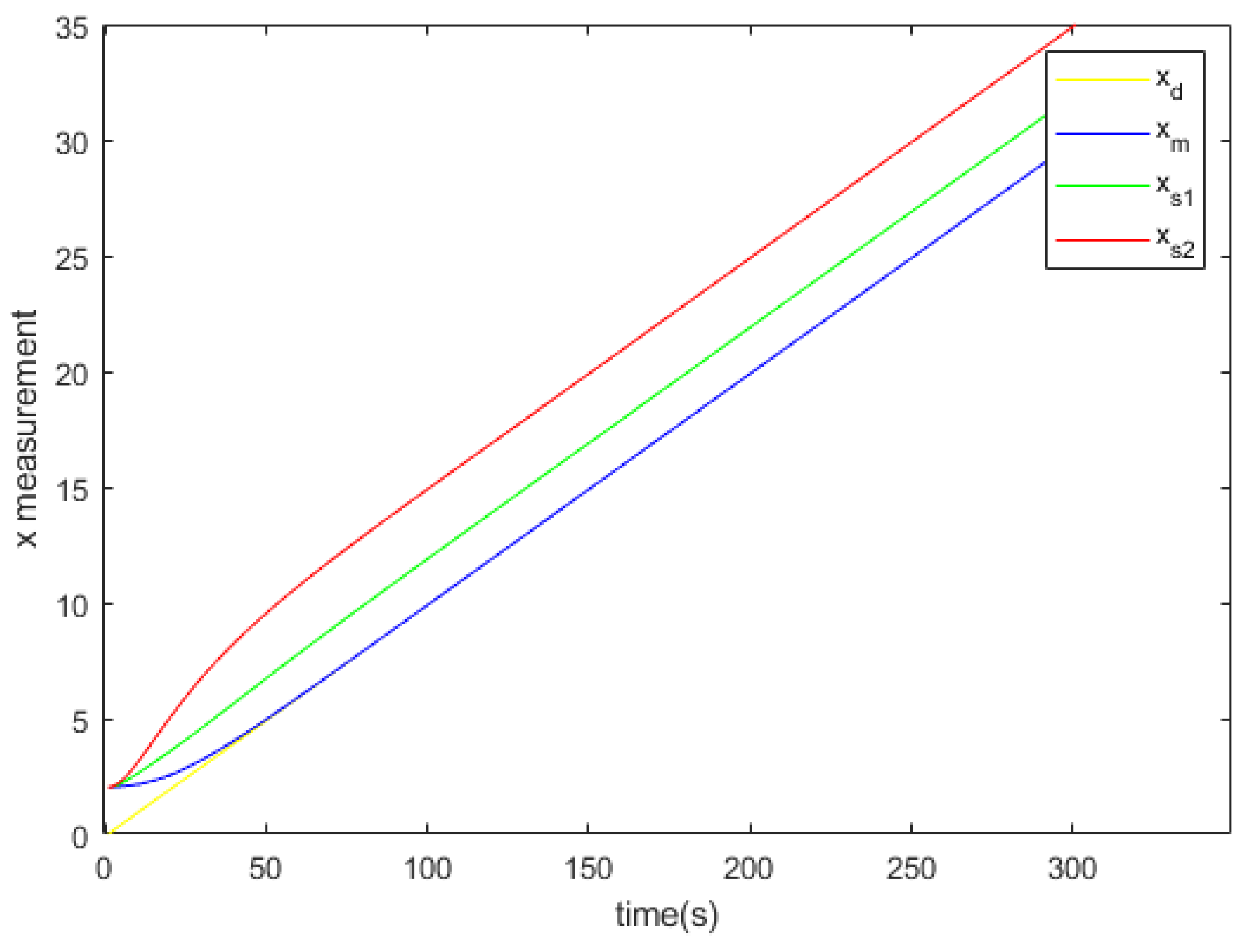
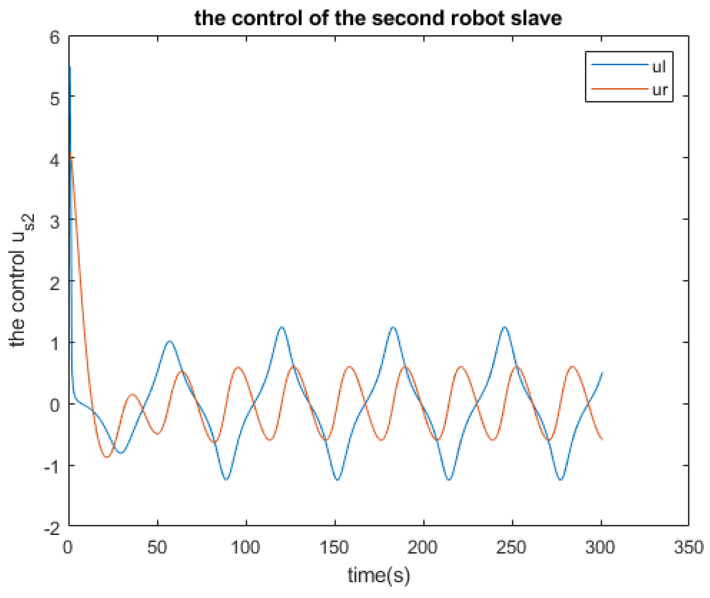
We get the responses of the master and the slaves shown in Figure 7 and Figure 8, also the control is shown in Figure 9, Figure 10 and Figure 11.

3. Fault Detection Based on the Extended Kalman Filter

3.1. Extended Kalman Filter and Fault Diagnosis

3.1.1. The Extended Kalman Filter (EKF)

In fact, fault detection means identifying and diagnosing malfunctions within a system. This involves recognizing deviations from the system’s normal or expected behavior, which could be indicative of faults such as sensor errors, actuator failures, process disturbances, or other issues affecting the system’s performance. Fault detection typically involves monitoring the system’s outputs and comparing them to the predicted values based on a model of the system’s normal operation. The extended Kalman filter (EKF) plays a crucial role in this process by providing a dynamic model that can estimate the system’s state variables and predict future outputs. Any significant discrepancies between the predicted and actual outputs can indicate the presence of a fault.
Within the extended Kalman filter framework, the nonlinearities inherent in the system dynamics are approximated using a linearized rendition of the nonlinear model based on the most recent state estimate. Let us consider the system characterized by the following state equations:
X ( k + 1 ) = f ( X , u , k ) + ρ ( k ) Y ( k + 1 ) = h ( X , u , k ) + γ ( k )
ρ ( k ) and γ ( k ) denote the process and observation noises, which are assumed to have a zero mean with covariances Ψ ρ k and Ψ γ k , respectively. Function f, defined as nonlinear according to Equation ( 7 ) , is employed to compute the predicted state from the previous estimate, as is function h for predicting the measurement from the predicted state. However, due to the nonlinearity of f and h, a Jacobian matrix of partial derivatives is computed, since these functions cannot be directly applied to the covariance.
  • Hypothesis:
As stated in [17], when the extended Kalman filter (EKF) is applied to a system and placed in a canonical observation form, it gains the following properties associated with global convergence:
  • The pair of matrices ( A , C ) is detectable, which means that there is no unstable mode or no observability in the system.
  • The signals ρ ( k ) and γ ( k ) are central Gaussian white noises. The Density Power Spectral (DSP) covariances Ψ ρ k and Ψ γ k mean
E [ γ ( i ) γ ( j ) T ] = Ψ ρ k , i f   i = j E [ ρ ( i ) ρ ( i ) T ] = Ψ γ k , i f   i = j E [ γ ( i ) ρ ( j ) T ] = 0 , i , j .
where E [ . . ] represents the mathematical expectation.
The latter equation illustrates the stochastic independence of the noises ρ and γ . This assumption is introduced to simplify the subsequent calculations but is not obligatory.
  • Correction:
  • Updated state estimate:
    x ^ k / k = x ^ k / k 1 + K k y ^ k
  • Updated covariance estimate:
    Ψ k / k = ( I K k C k ) Ψ k / k 1
  • Measurement residual:
    y ˜ k = y k C k x ^ k / k 1
  • Innovation covariance:
    Z k = C k Ψ k / k 1 C k T + Ψ γ k
  • Near-optimal Kalman gain:
    K k = Ψ k / k 1 C k T Z k 1
  • Prediction:
  • Predicted state estimate:
    x ^ k + 1 / k = A k x ^ k / k + u k
  • Predicted covariance:
    Ψ k + 1 / k = A k Ψ k / k A k T + Ψ ρ k
where A k is the linearized matrix of the function f, which is written as follows:
A k = δ f δ X | x ^ k / k
Remark 1.
Occasionally, numerical issues can cause the covariance of innovation Z k to lose its positive definite nature. In such instances, it is advisable to substitute the equation for covariance estimation with
Ψ k / k = ( I K k C k ) Ψ k / k 1 Ψ k / k 1 T ( I K k C k ) T
The replacement will always ensure a positive, definite outcome, even if the matrix Ψ k / k 1 is not. Consequently, the Kalman equations will exhibit greater stability, as any minor deviations in the positive definite nature of the covariance matrices will be corrected in the subsequent iteration. According to ( 14 ) ,
A k = 1 0 T e v sin ( θ ) cos ( θ ) 0 1 T e v cos ( θ ) sin ( θ ) 0 0 1 0 0 0 0 1
Suppose that the signals γ k and ρ k are Gaussian white noise with a unit covariance matrix; that is to say,
Ψ γ = 1 0 0 1 Ψ ρ = 1 0 0 0 0 1 0 0 0 0 1 0 0 0 0 1
Also, we take the sample time T e = 0.01 .

3.1.2. Fault Diagnosis Steps

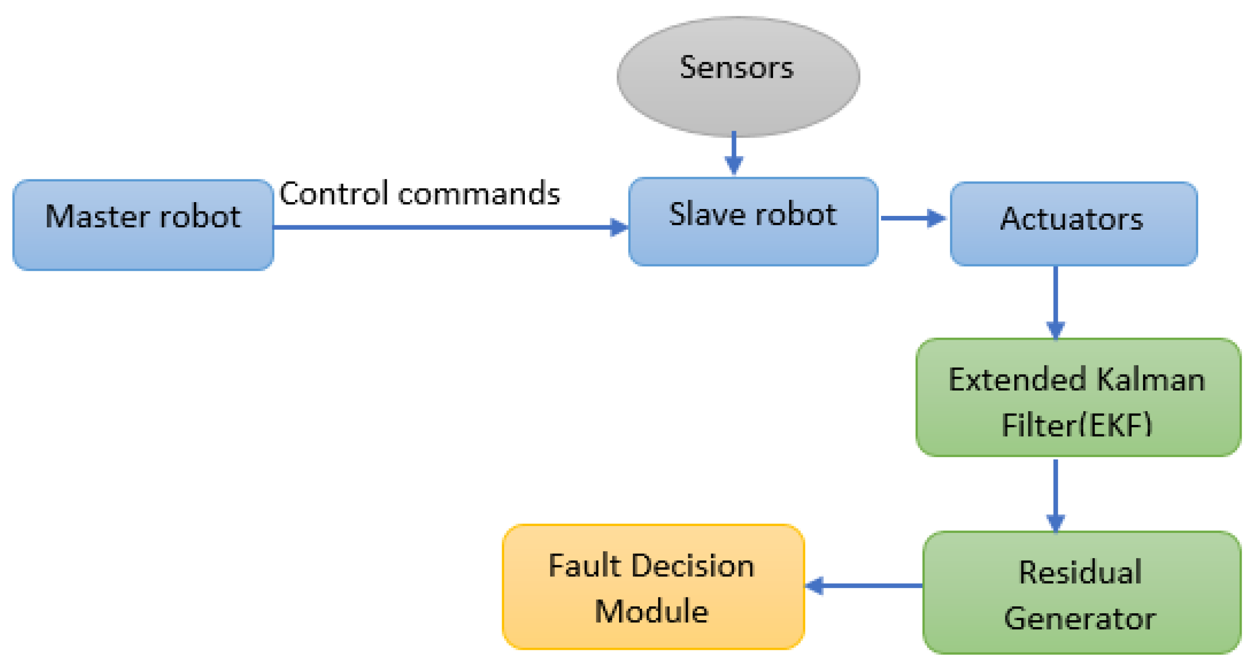
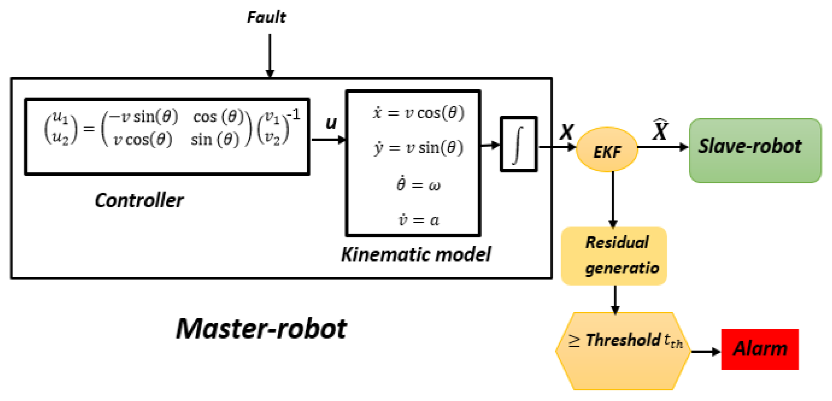
Figure 12 describes the fault detection procedure in the master–salve robot configuration.
This configuration has the following components:
  • Master Robot: Sends control commands to the Slave Robot.
  • Slave Robot: Execute actions based on the received commands.
  • Sensors: Collect data from the environment and the robots’ states, providing inputs for the EKF.
  • Actuators: Perform the necessary actions in response to control signals.
  • Extended Kalman Filter (EKF): Estimates the system’s states based on sensor data and predicted models.
  • Residual Generator: Calculates residuals by comparing the EKF’s state estimates with actual measurements.
  • Fault Decision Module: Analyzes the residuals to detect any discrepancies indicating potential faults, triggering appropriate responses if faults are detected.
Generally, a fault diagnosis system follows three steps: a residual generation, a residue evaluation, and a decision logic [18].
  • Step 1: Residual generation
The residual generator generates a fault indicator vector, or residual vector, denoted r, based on the measurements of the input and output variables of the system. The nominal value of the residue, excluding transient effects, is theoretically equal to zero under the normal operating conditions of the monitored system. When a fault appears, this residual moves away from zero depending on the fault.
  • Step 2: Residue evaluation
The residual evaluation module consists of measuring the residue and determining whether the system is functioning properly or not using specific algorithms and methods [18]. Detecting a fault typically involves comparing the residues with a predetermined detection threshold t t h . This threshold represents a crucial aspect of residual-based FDI methods, defined as the boundary value for the deviation of a residue from zero. Thus, the process of fault detection proceeds as follows:
r = 1 i f , r > | t t h | 0 i f , r < | t t h | .
Excessively high thresholds may result in failing to detect a fault (missed alarm), while overly low thresholds may lead to false alarms, detecting faults in healthy conditions [19]. There exist two categories of thresholds [8]: the first being a constant threshold, and the second, an adaptive one. The adaptive threshold is employed to accommodate the inevitable parameter uncertainty, disturbances, and noise encountered in practical applications.
  • Step 3: Decision
This step involves examining the outcome of evaluating a set of residues, and, based on the pattern of activated and non-activated tests, it generates a determination regarding the faulty component within the monitored system.

3.2. Closed-Loop System

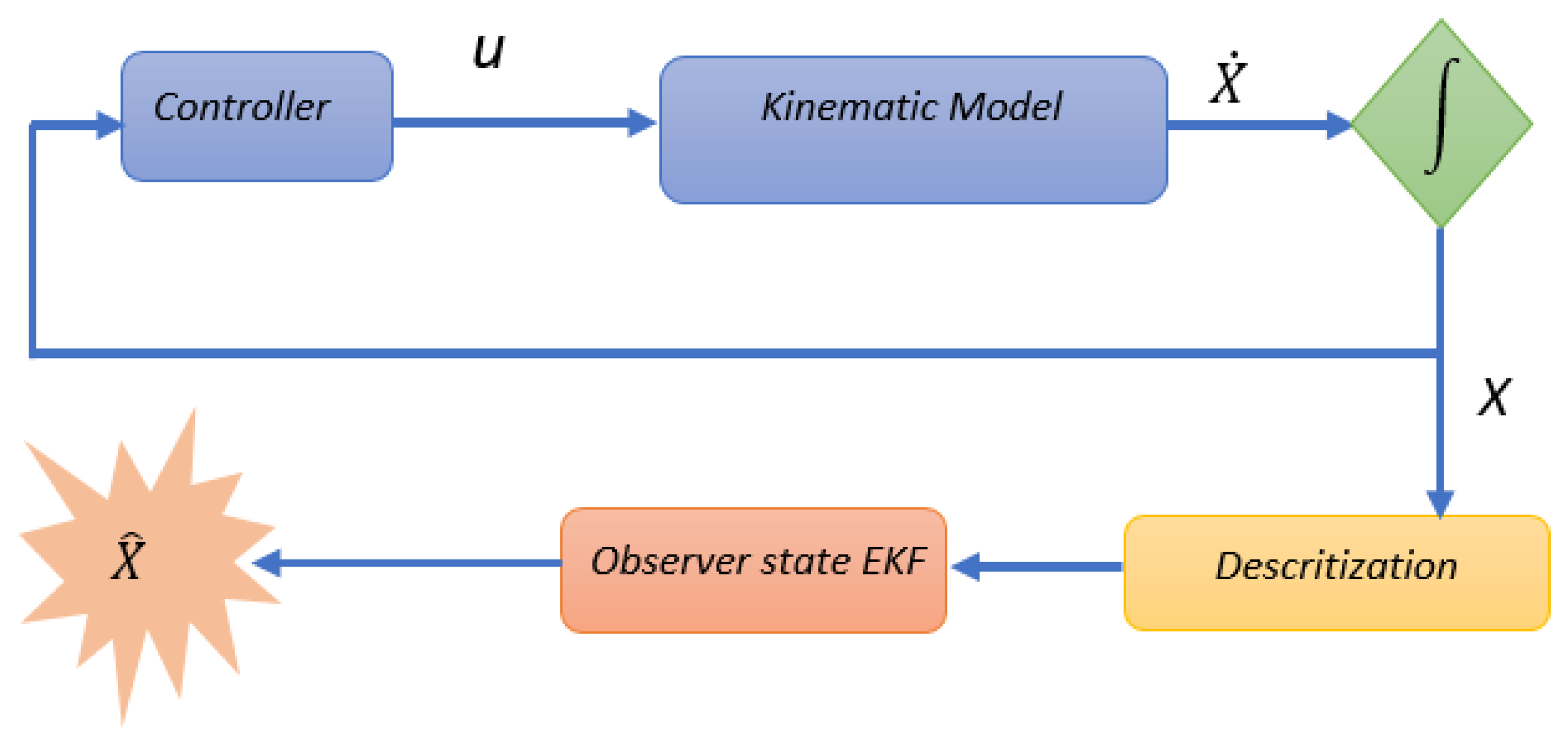
The closed-loop system was used in Simulink/Matlab and is shown in the functional diagram in Figure 13.
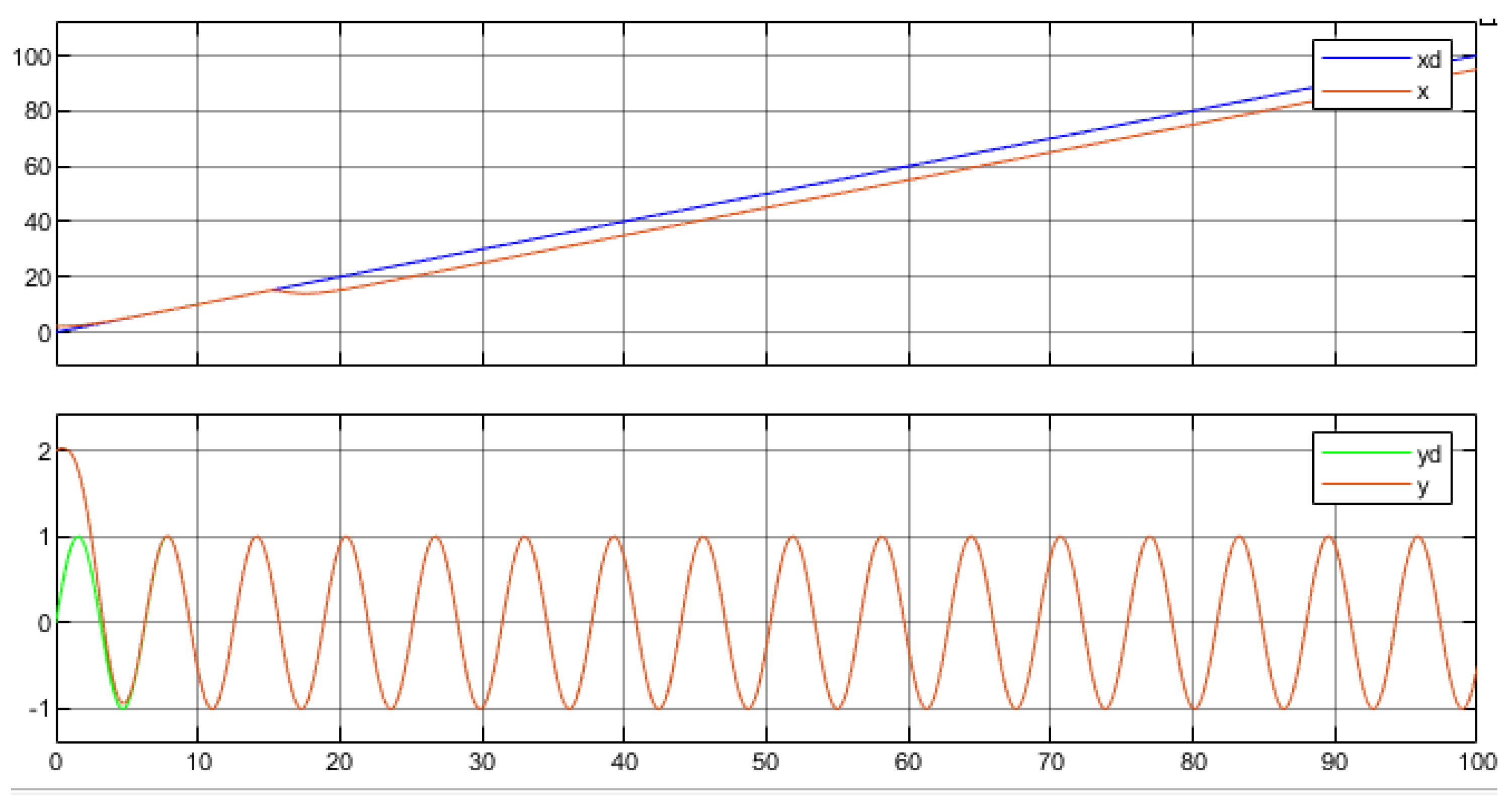
The robot was controlled in order to follow a desired trajectory given by P d = [ x d , y d ] T , as shown in Figure 14.

3.3. Simulation Results

We noticed that the robot master follows the desired trajectory (see Figure 15).
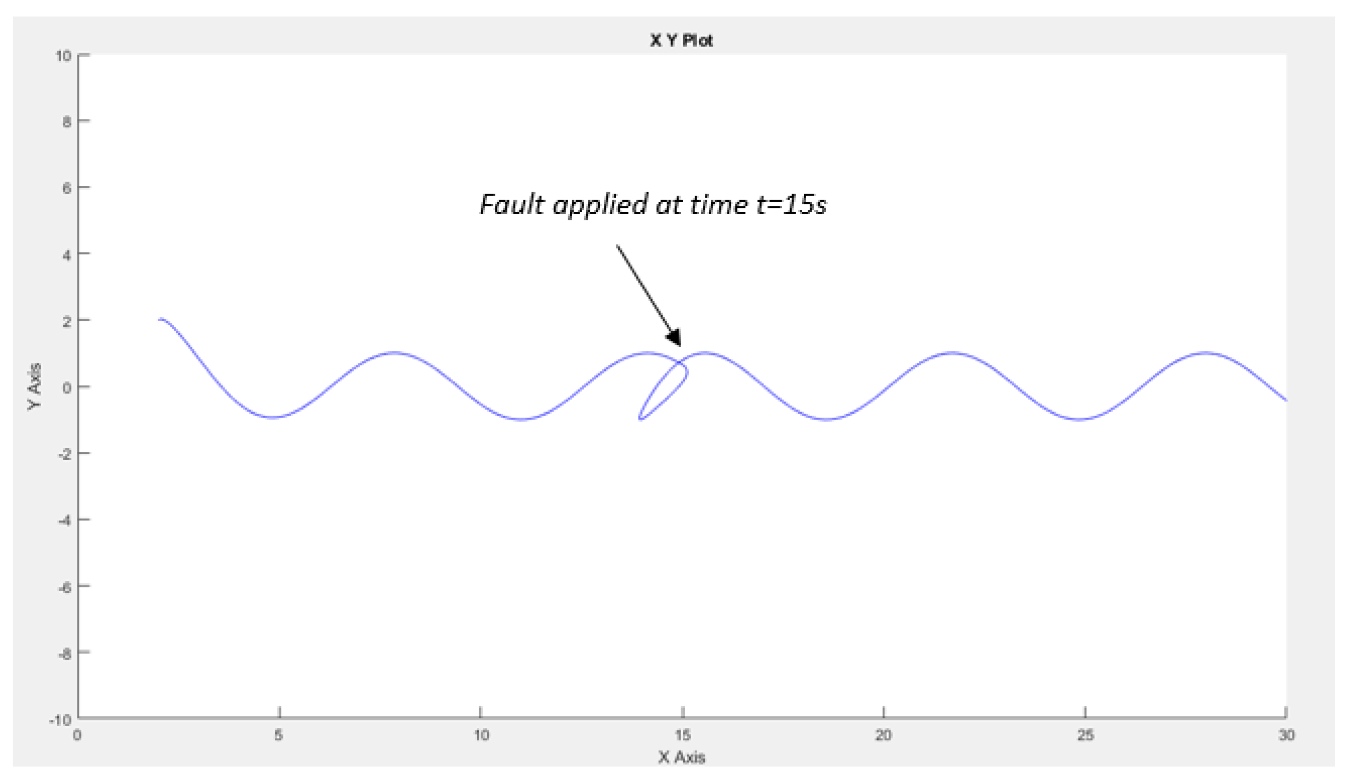
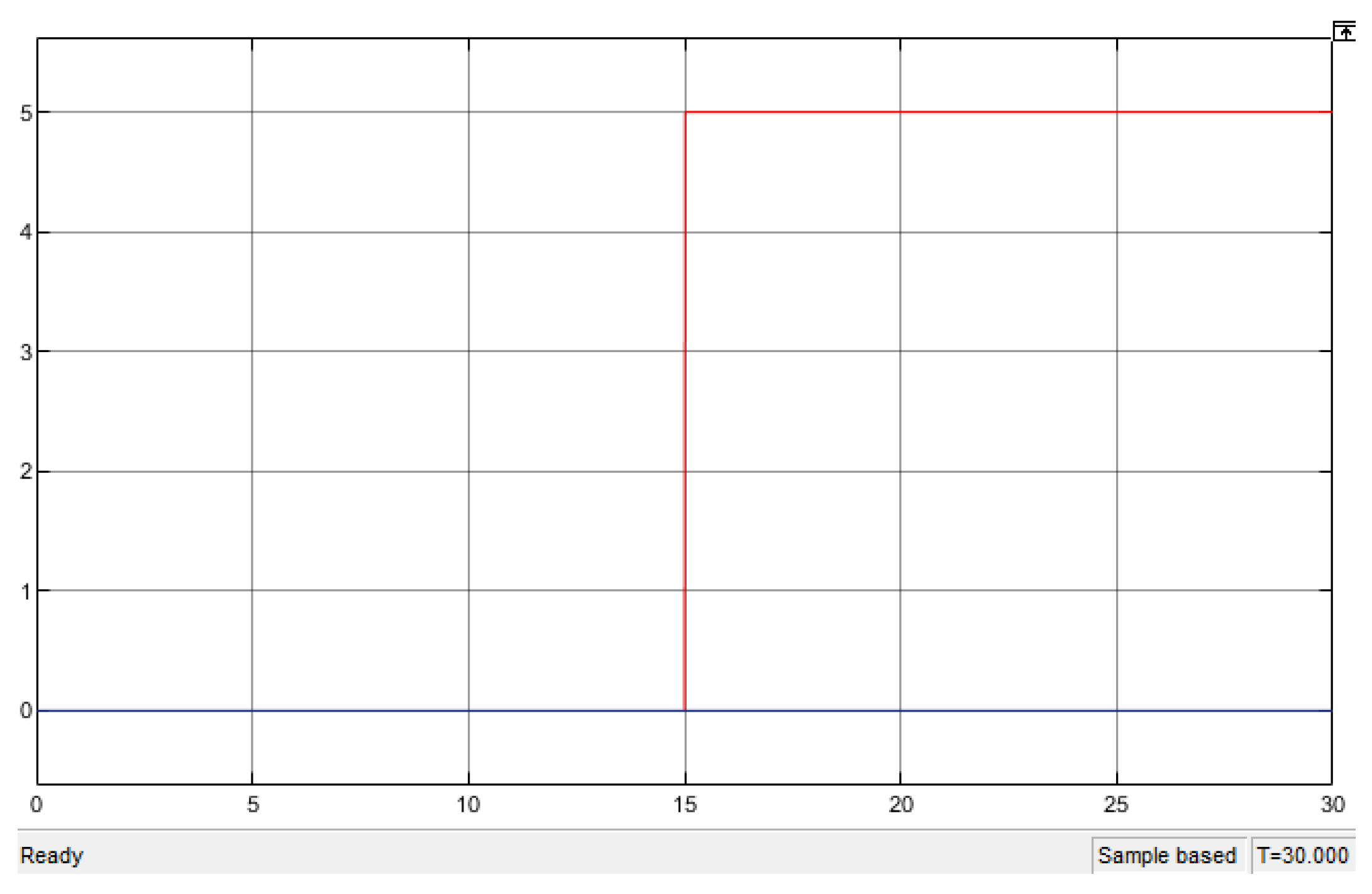
The fault scenario addressed involves an offset applied to the x measurement at the 15 s mark. Subsequently, we applied our Extended Kalman Filter (EKF), and the resulting robot trajectory is illustrated in Figure 16.
It is observed that there is a slight deviation attributable to the applied fault, yet the robot continues to track the same trajectory consistently.
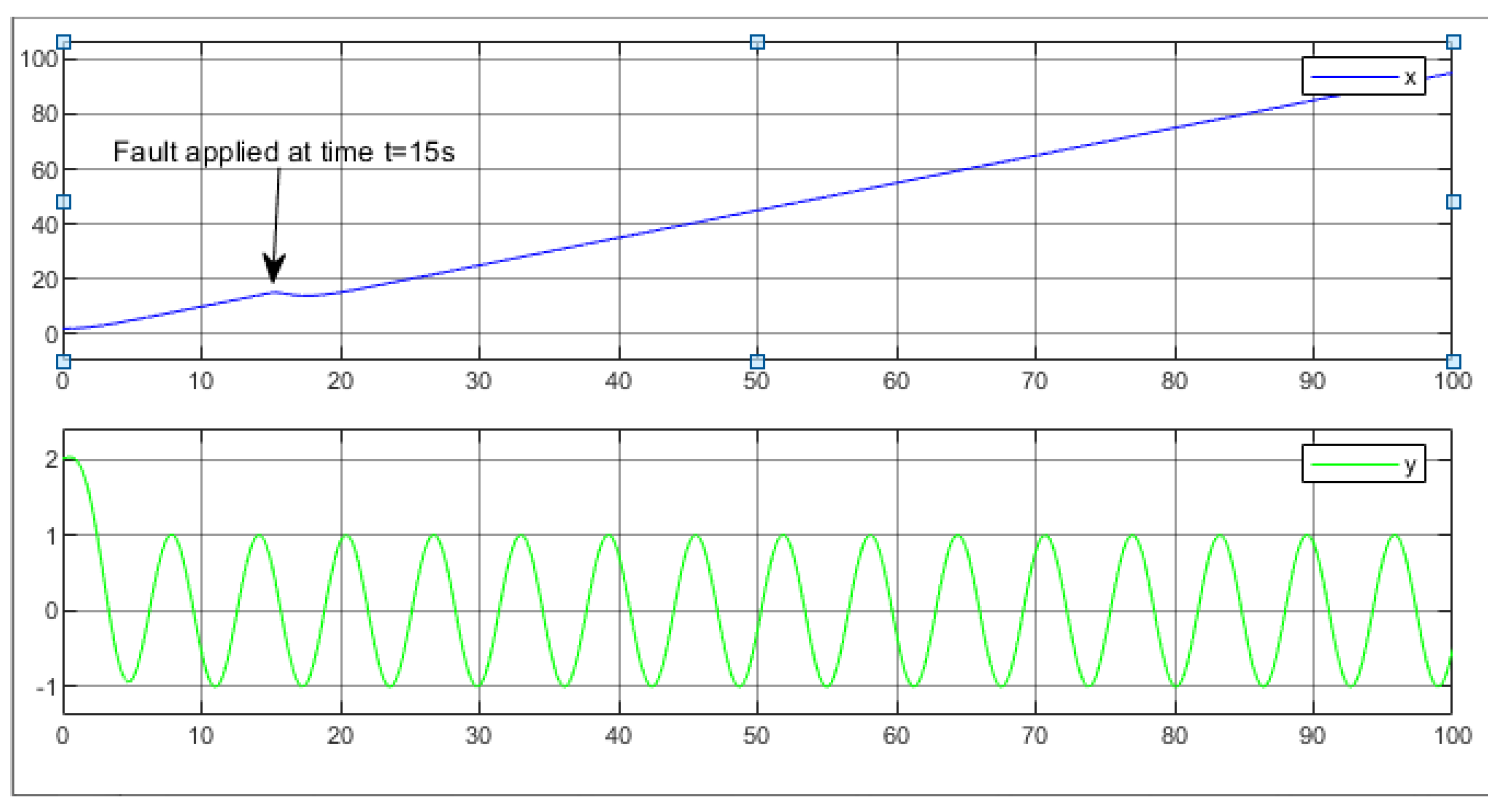
Furthermore, upon introducing a fault (considered an intermittent fault, such as a switch) to a parameter at time t = 15 s, a minor peak is observed (see Figure 17), after which the robot promptly returns to its intended trajectory. Hence, it can be concluded that the Extended Kalman Filter effectively identifies the fault introduced into the system.

4. Fault Detection in Multi-Robot System

In the preceding section, the system (consisting of a robot master and slaves) executes its trajectory within an ideal environment. However, real-world environments lack such ideal conditions. Thus, we aimed to introduce a fault and observe how the system responds to the challenge. Indeed, the multi-robot system under fault is described in the following figure (see Figure 18). It was observed that the robot master adheres to its trajectory, as depicted in Figure 3.
Subsequently, we induced an offset fault in the master robot’s x measurement at 15 s, as illustrated in Figure 19.
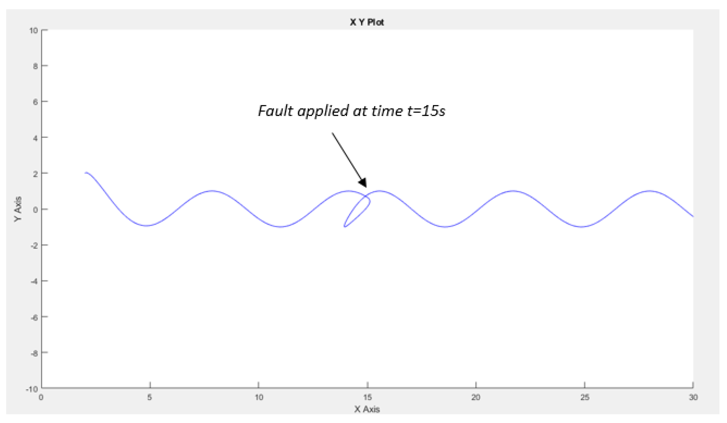
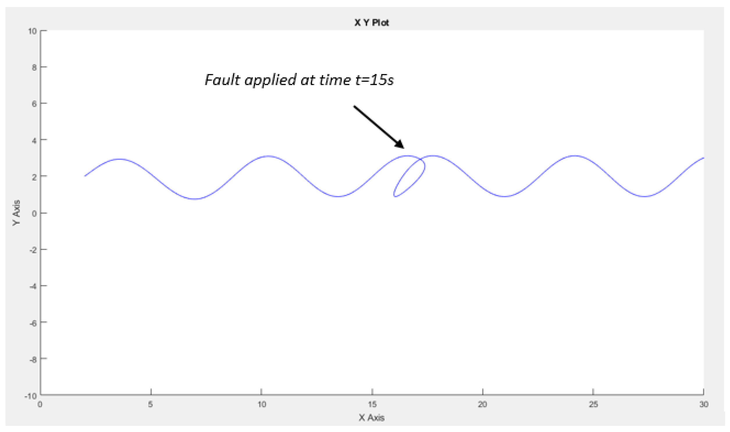
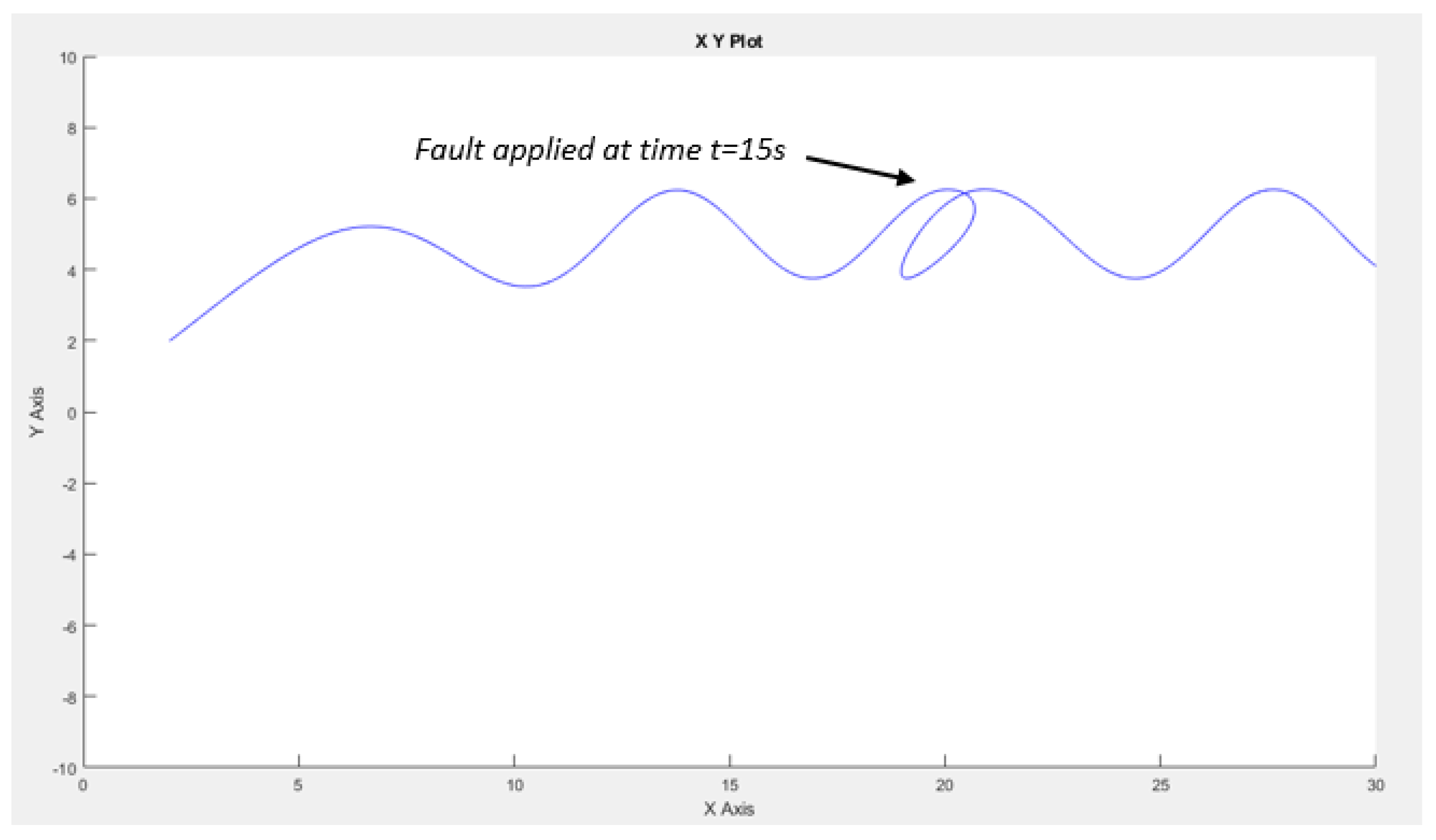
The responses of both the master and the slaves are depicted in the subsequent figures (Figure 20, Figure 21 and Figure 22). It is observed that the trajectory of the robots experiences a slight disturbance at a specific time, yet it promptly returns to its intended path without deviating from the desired trajectory.
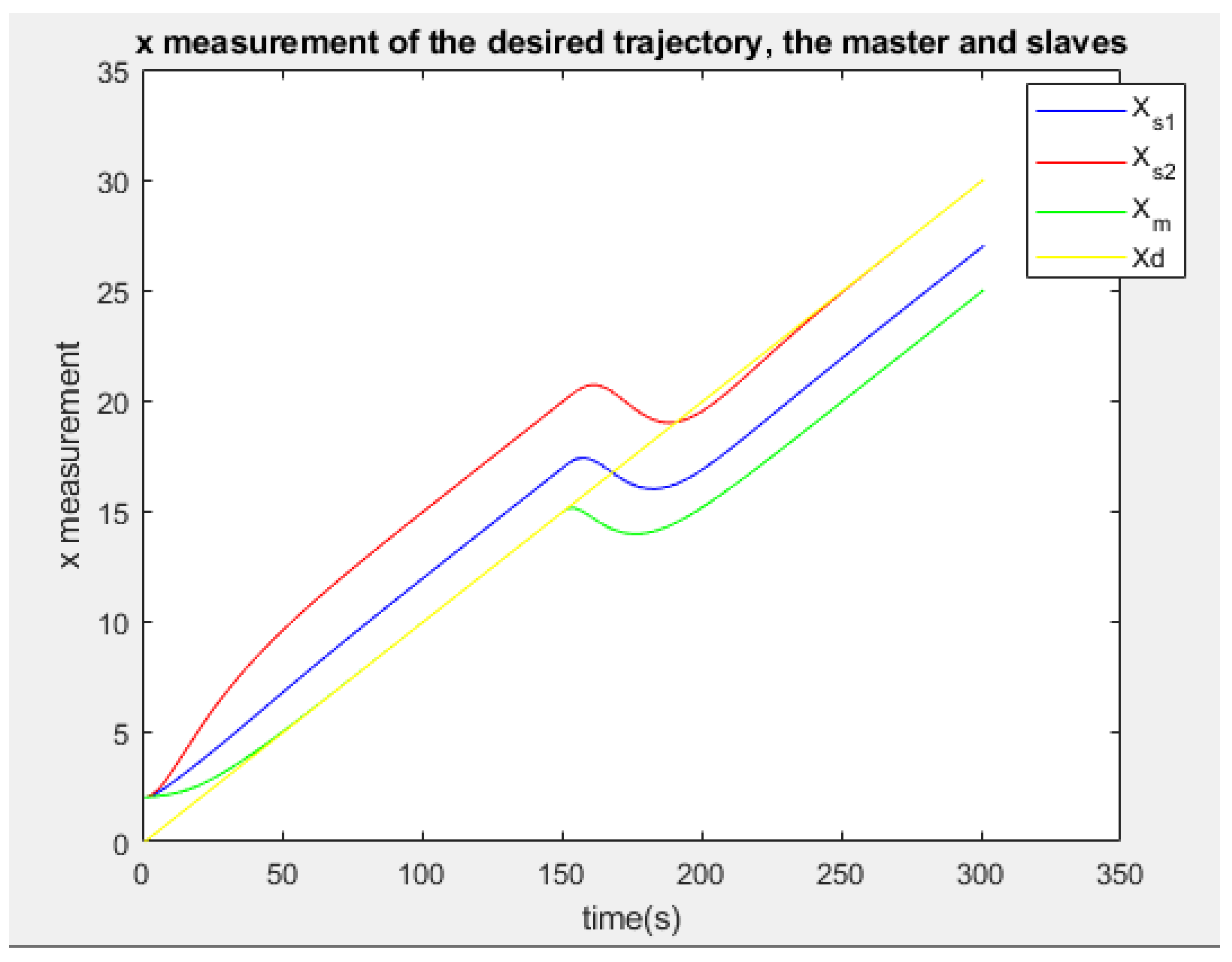
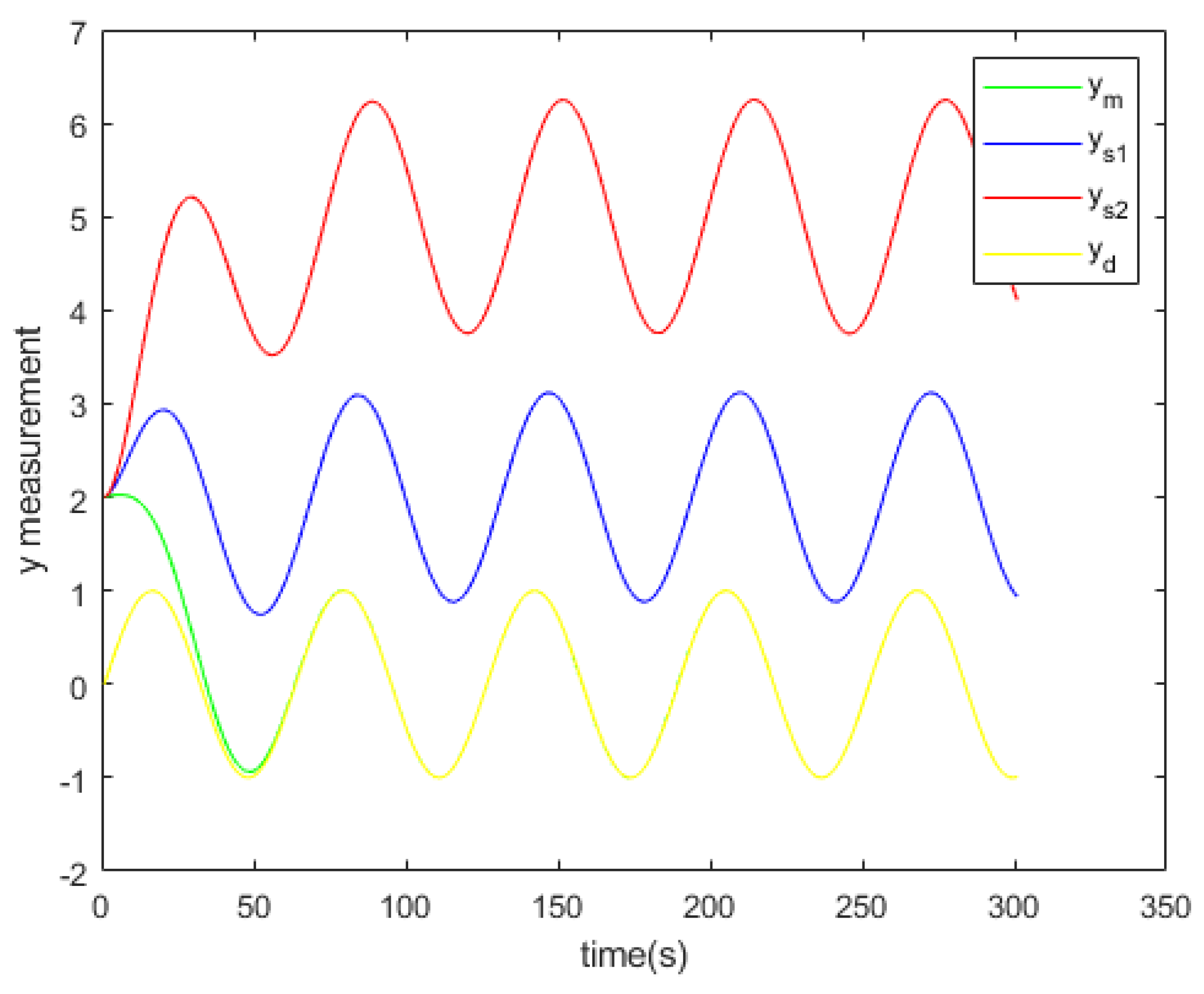
Figure 23 and Figure 24 show the x and y measurements of the desired trajectory, the master and the slaves, respectively.
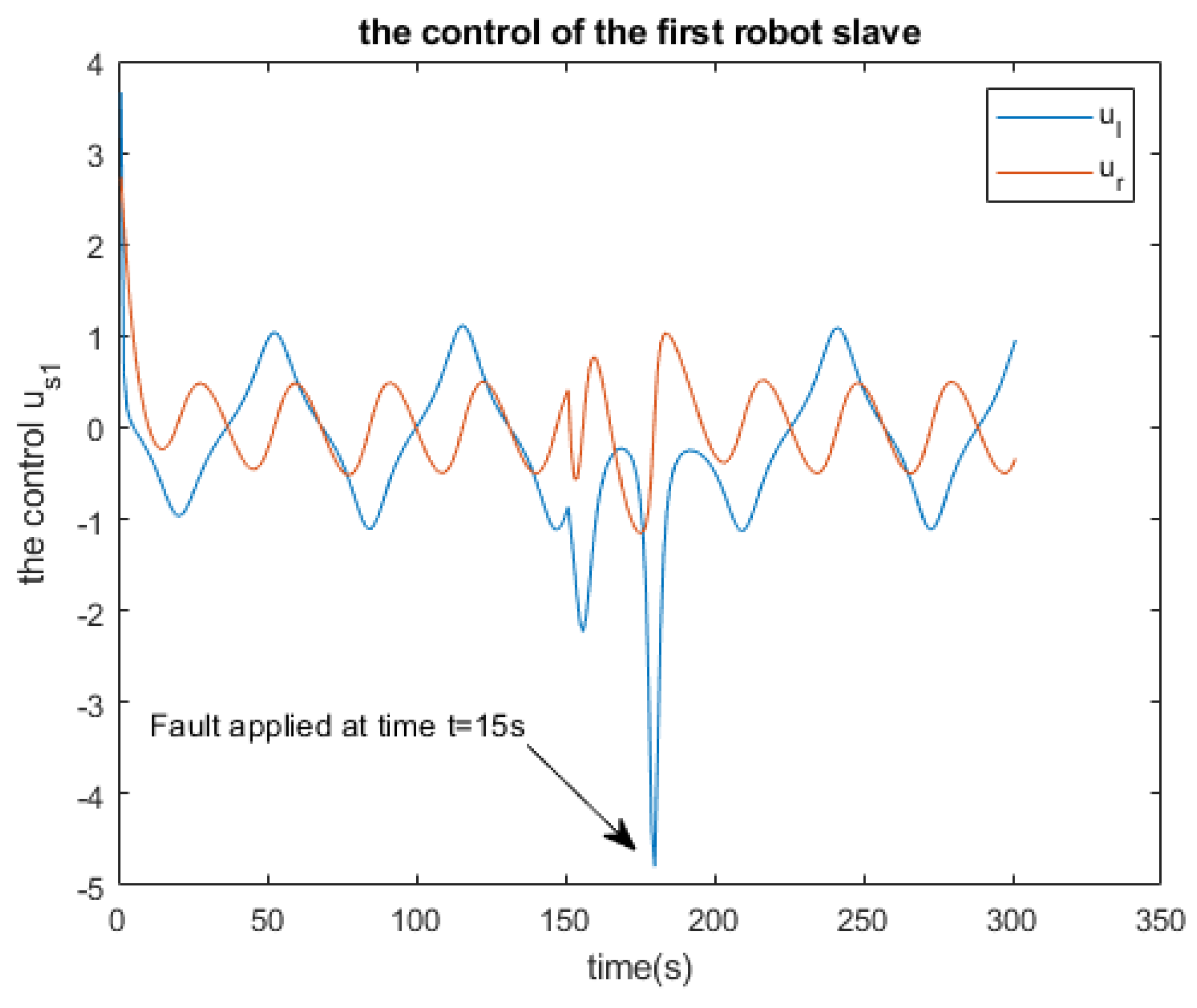
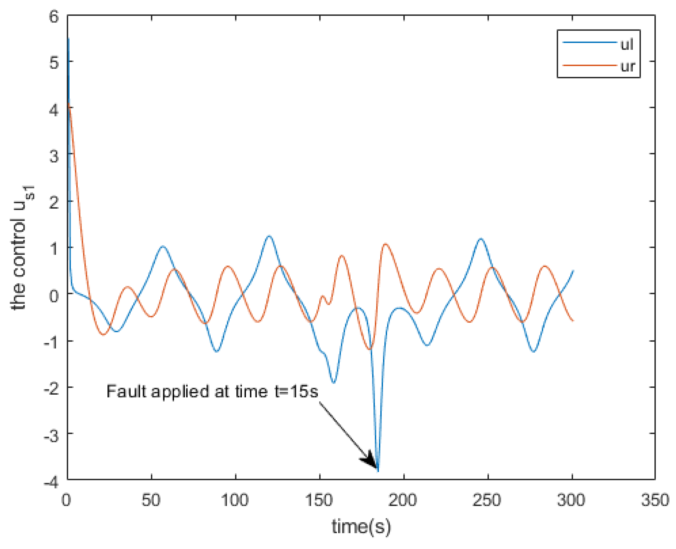
Furthermore, the simulations of the controllers for both the master and the slaves are illustrated in Figure 25, Figure 26 and Figure 27, respectively. It is observed that the robot master adheres to the desired trajectory until time t = 15 s, at which point it deviates slightly. However, after a few seconds, it resumes following the trajectory initially set.
Meanwhile, our attention is directed toward the behaviors of the robot slaves, which entail two cases for investigation: firstly, when a robot slave operates without fault, and secondly, when a robot slave is subjected to a fault injection. The simulations depicted in Figure 21 and Figure 22 revealed the impact on the functionality of the slave robot. Notably, a minor peak is observed in the slave responses (refer to Figure 23 and Figure 24), following which it swiftly resumes its trajectory.

Fault Diagnosis

To utilize the extended Kalman filter (EKF) for fault detection in a wheeled mobile robot, the following procedural steps are advised:
1- System Modeling: Develop a comprehensive model that characterizes the robot’s behavior under both normal operating conditions and various fault scenarios.
2- State Estimation: Implement the EKF to estimate the current state of the robot utilizing sensor measurements.
3- Fault Models: Define specific fault models detailing how each fault impacts the robot’s state and sensor measurements.
4- Residual Calculation: Calculate residuals by computing the disparity between actual measurements and estimated measurements, based on the fault models delineated in the preceding step.
5- Fault Detection: Employ statistical tests or threshold-based techniques on the residuals to identify the occurrence of faults.
6- Fault Diagnosis: Initiate the fault diagnosis phase subsequent to the detection of faults.
For establishing thresholds, the system should first undergo simulations under fault-free conditions, followed by simulations with faults. The fault-free simulations aid in determining thresholds t t h through the application of the three-sigma method:
t t h = 3 σ + t t h = + 3 σ
where σ denotes the standard deviation of residual r.
Note that σ reflects the EKF accuracy and is calculated based on the EKF error:
σ = 1 n i = 1 n ( e i 2 )
As mentioned in the previous section, the fault is said to be detected when the residual exceeds the threshold more than | t t h | .
Based on the EKF in our case, we calculated the difference between the values of the robot’s state vector and the values of the estimated state vector X e . So four residuals are generated for each robot:
r x = x x e r y = y y e r θ = θ θ e r v = v v e
where the index e means the estimated value. Each residual is compared to the threshold.
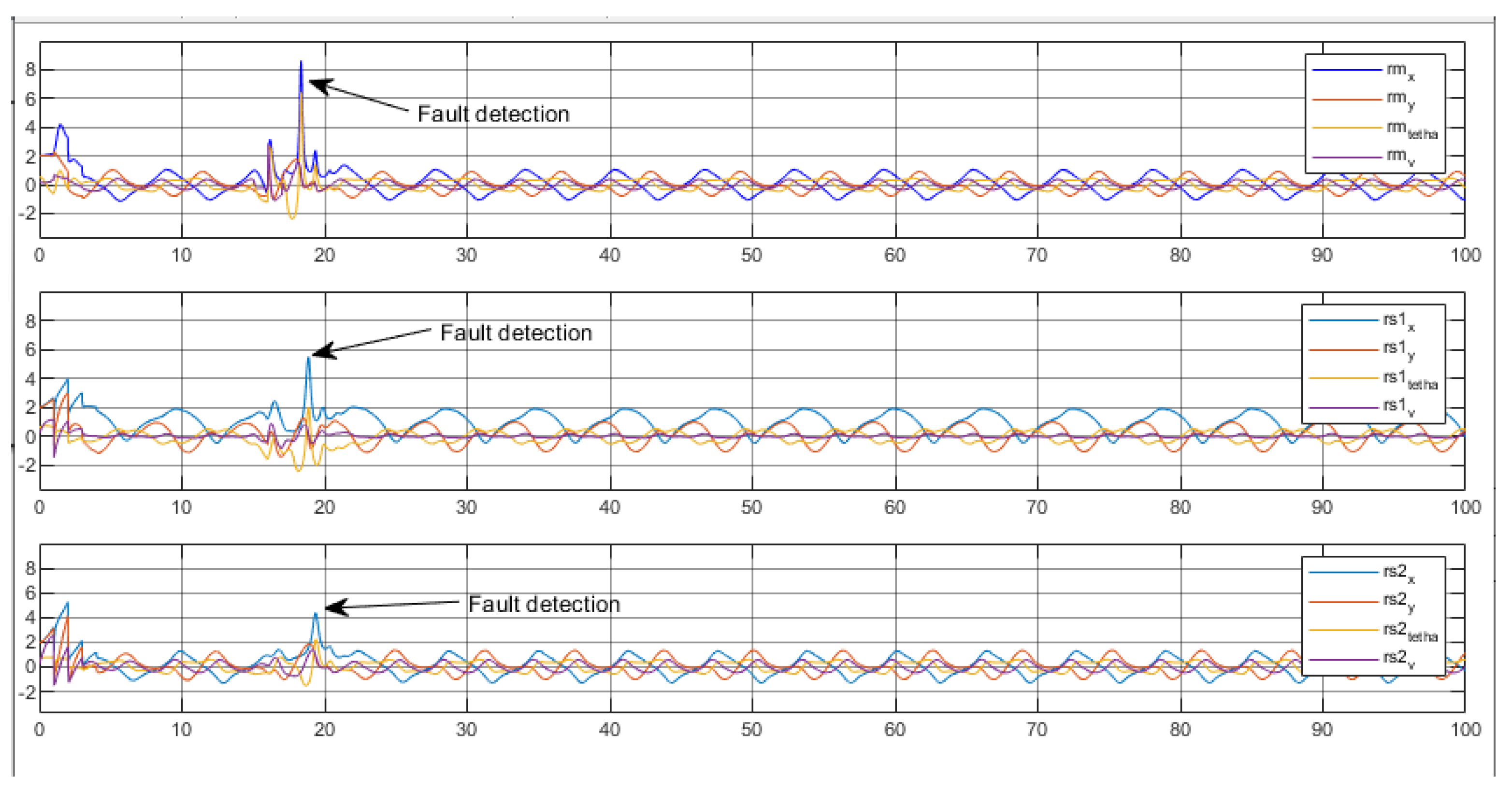
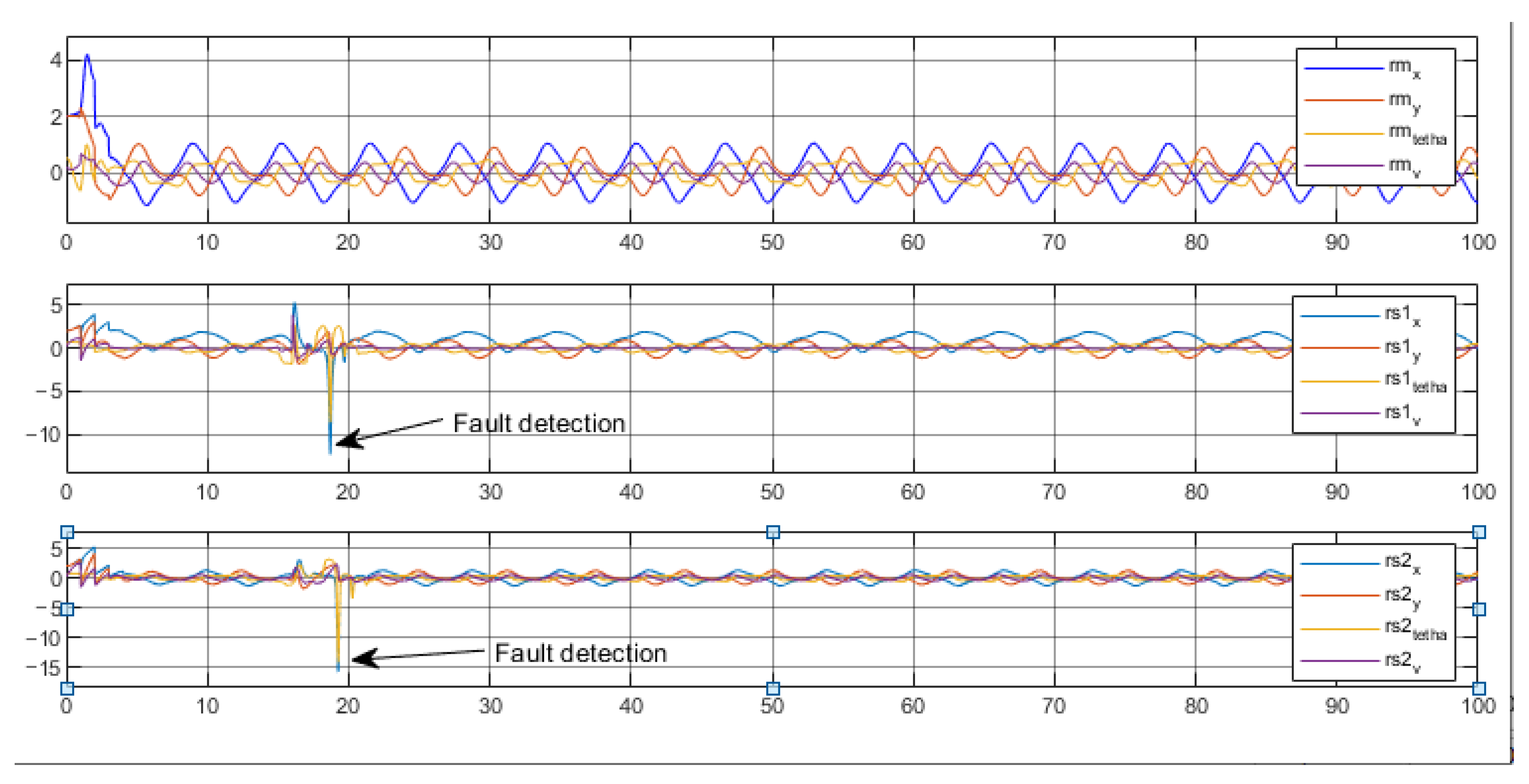
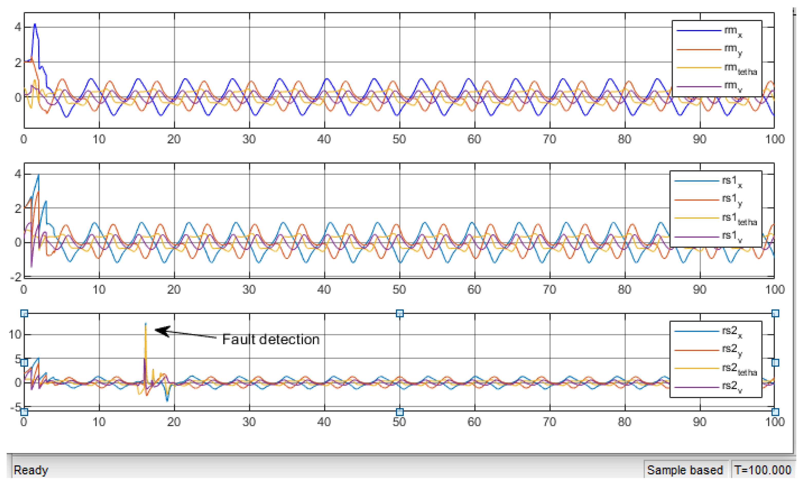
Table 1 summarizes the signatures of the residuals under a fault applied to the robot master and the slave robots. The different residual signatures allow for fault isolation. We notice that when the fault appears in the robot master, the other two robots (slaves) are affected. On the other side, if we insert the fault in the robot slaves, the master is not affected, so we conclude that the fault affects only the following robots. Hence, we can say that the fault propagates in one direction only. As shown in the figures (Figure 28, Figure 29 and Figure 30), a fault appears at time t = 15 s and is detected, and the detection delay does not affect the system performance.

5. Conclusions

In this paper, we consider the architecture of a network of three robots, with a master and two slaves working in consensus. The main task is assigned to the master, and the two slaves follow. Graph theory is used to model the whole system. Next, in order to continuously estimate the state of each robot, an extended Kalman filter is assigned to each robot. The residual generator compares the current state of the robot with its estimated state. It deduces whether a fault has occurred or not. We noticed that faults propagate from the master to the slaves according to the orientation of the arcs in the graph. In analyzing the fault signature table and the adjacency matrix (A), this observation allowed us to isolate faulty robots. The problem becomes more complex when the graph is not a directed graph. In this case, a temporal analysis of the moment of fault occurrence is mandatory. This is our perspective for future work.

Author Contributions

Conceptualization, A.J. and B.B.; methodology, A.J. and B.B.; software, A.Z.; validation, B.B., A.Z. and M.N.A.; formal analysis, A.J.; investigation, A.J. and B.B.; resources, A.J.; data curation, B.B.; writing—original draft preparation, A.J. and B.B.; writing—review and editing, A.J. and B.B.; visualization, B.B.; supervision, A.Z.; project administration, M.N.A.; funding acquisition A.J. All authors have read and agreed to the published version of the manuscript.

Funding

This research received no external funding.

Data Availability Statement

The data presented in this study are available on request from the corresponding author due to (specify the reason for the restriction).

Conflicts of Interest

The authors declare no conflicts of interest.

References

  1. Ribeiro, A.F.A.; Lopes, A.C.C.; Ribeiro, T.A.; Pereira, N.S.S.M.; Lopes, G.T.; Ribeiro, A.F.M. Probability-Based Strategy for a Football Multi-Agent Autonomous Robot System. Robotics 2024, 13, 5. [Google Scholar] [CrossRef]
  2. Guo, X.G.; Xu, W.D.; Wang, J.L.; Park, J.H. Distributed neuroadaptive fault-tolerant sliding-mode control for 2-D plane vehicular platoon systems with spacing constraints and unknown direction faults. Automatica 2021, 129, 109675. [Google Scholar] [CrossRef]
  3. Ruch, C.; Gachter, J.; Hakenberg, J.; Frazzoli, E. The +1 Method: Model-Free Adaptive Repositioning Policies for Robotic Multi-Agent Systems. IEEE Trans. Netw. Sci. Eng. 2020, 7, 3171–3184. [Google Scholar] [CrossRef]
  4. Engelmann, D.C.; Ferrando, A.; Panisson, A.R.; Ancona, D.; Bordini, R.H.; Mascardi, V. RV4JaCamdash;Towards Runtime Verification of Multi-Agent Systems and Robotic Applications. Robotics 2023, 12, 49. [Google Scholar] [CrossRef]
  5. Jouili, A.; Boussaid, B.; Zouinkhi, A.; Abdelkrim, M. Finite time consensus for multi-tricycle systems under graph theory. In Proceedings of the 2020 20th International Conference on Sciences and Techniques of Automatic Control and Computer Engineering (STA), Sfax, Tunisia, 20–22 December 2020; pp. 24–29. [Google Scholar] [CrossRef]
  6. Sayed-Mouchaweh, M.; Billaudel, P. Abrupt and Drift-Like Fault Diagnosis of Concurent Discrete Event Systems. In Proceedings of the 2012 11th International Conference on Machine Learning and Applications, Boca Raton, FL, USA, 12–15 December 2012; Volume 2, pp. 434–439. [Google Scholar] [CrossRef]
  7. Khan, A.Q. Observer-Based Fault Detection in Nonlinear Systems. Ph.D. Thesis, University of Duisburg Essen, Essen, Germany, 2010. [Google Scholar]
  8. Sallem, F. Détection et Isolation de Défauts Actionneurs Basées sur un Modèle de L’organe de Commande. Ph.D. Thesis, Université Paul Sabatier—Toulouse III, Toulouse, France, 2013. [Google Scholar]
  9. Mouzakitis, A. Classification of fault diagnosis methods for control systems. Meas. Control. 2013, 46, 303–308. [Google Scholar] [CrossRef]
  10. Fourlas, G.K.; Karras, G.C.; Kyriakopoulos, K.J. Sensors fault diagnosis in autonomous mobile robots using observer —Based technique. In Proceedings of the 2015 International Conference on Control, Automation and Robotics, Singapore, 20–22 May 2015; pp. 49–54. [Google Scholar] [CrossRef]
  11. Yutian, L.; Jungan, C. Integrated Fault Diagnosis Method of Mobile Robot. In Theoretical and Mathematical Foundations of Computer Science; Springer: Berlin/Heidelberg, Germany, 2011; pp. 372–379. [Google Scholar]
  12. Rhouma, T.; Keller, J.Y.; Abdelkrim, M.N. A Kalman filter with intermittent observations and reconstruction of data losses. Int. J. Appl. Math. Comput. Sci. 2022, 32, 241–253. [Google Scholar] [CrossRef]
  13. Ducard, G. Smac–Fdi: A Single Model Active Fault Detection and Isolation System for Unmanned Aircraft. Int. J. Appl. Math. Comput. Sci. 2015, 25, 189–201. [Google Scholar] [CrossRef]
  14. Jouili, A.; Boussaid, B.; Zouinkhi, A.; Abdelkrim, M. Fault detection in wheeled mobile robot based on extended kalman filter. In Proceedings of the 2022 IEEE 21st international Ccnference on Sciences and Techniques of Automatic Control and Computer Engineering (STA), Sousse, Tunisia, 19–21 December 2022; pp. 237–242. [Google Scholar]
  15. Jouili, A.; Boussaid, B.; Zouinkhi, A.; Abdelkrim, M.N. FDI based extended kalman filter for multi robot system. In Proceedings of the 2023 20th International Multi-Conference on Systems, Signals & Devices (SSD), Mahdia, Tunisia, 20–23 February 2023; pp. 675–680. [Google Scholar] [CrossRef]
  16. Kia, S.S.; Van Scoy, B.; Cortes, J.; Freeman, R.A.; Lynch, K.M.; Martinez, S. Tutorial on Dynamic Average Consensus: The Problem, Its Applications, and the Algorithms. IEEE Control Syst. Mag. 2019, 39, 40–72. [Google Scholar] [CrossRef]
  17. Boizot, N.; Busvelle, E.; Jean-Paul, G. An adaptive high-gain observer for nonlinear systems. Automatica 2010, 46, 1483–1488. [Google Scholar] [CrossRef]
  18. Bokor, J.; Szabo, Z. Fault detection and isolation in nonlinear systems. Annu. Rev. Control 2009, 33, 113–123. [Google Scholar] [CrossRef]
  19. Samia, M.; Graton, G.; El Mostafa, E.; Ouladsine, M.; Planchais, A. On fault detection and isolation applied on unicycle mobile robot sensors and actuators. In Proceedings of the 2018 7th International Conference on Systems and Control (ICSC), Valencia, Spain, 24–26 October 2018; pp. 148–153. [Google Scholar]
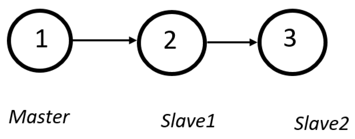
Figure 1. Directed graph.
Actuators 13 00253 g001
Figure 2. Geometry of a unicycle robot.
Actuators 13 00253 g002
Figure 3. The desired trajectory.
Actuators 13 00253 g003
Figure 4. The robot master’s trajectory.
Actuators 13 00253 g004
Figure 5. The first robot slave’s trajectory.
Actuators 13 00253 g005
Figure 6. The second robot slave’s trajectory.
Actuators 13 00253 g006
Figure 7. The x coordinate of the desired trajectory of the master and the slaves.
Actuators 13 00253 g007
Figure 8. The y coordinate of the desired trajectory of the master and the slaves.
Actuators 13 00253 g008
Figure 9. The control of the robot master.
Actuators 13 00253 g009
Figure 10. The control of the first robot slave.
Actuators 13 00253 g010
Figure 11. The control of the second robot slave.
Actuators 13 00253 g011
Figure 12. A block diagram illustrating fault detection in a master–slave robot system.
Actuators 13 00253 g012
Figure 13. Unicycle mobile robot closed loop.
Actuators 13 00253 g013
Figure 14. Desired trajectories x d and y d .
Actuators 13 00253 g014
Figure 15. Coordinates x and y of the desired trajectory and the mobile robot.
Actuators 13 00253 g015
Figure 16. Trajectory of the mobile robot when fault applied at t = 15 s.
Actuators 13 00253 g016
Figure 17. Coordinates x and y of the mobile robot when fault applied at t = 15 s.
Actuators 13 00253 g017
Figure 18. Multi-robot system closed loop.
Actuators 13 00253 g018
Figure 19. The fault applied at time t = 15 s.
Actuators 13 00253 g019
Figure 20. The trajectory of the robot master with fault applied at time t = 15 s.
Actuators 13 00253 g020
Figure 21. The trajectory of the first robot slave with fault applied at time t = 15 s.
Actuators 13 00253 g021
Figure 22. The trajectory of the second robot slave with fault applied at time t = 15 s.
Actuators 13 00253 g022
Figure 23. The coordinate x of the desired trajectory of the master and slaves.
Actuators 13 00253 g023
Figure 24. The coordinate y of the desired trajectory of the master and slaves.
Actuators 13 00253 g024
Figure 25. The control of the robot master.
Actuators 13 00253 g025
Figure 26. The control of the first robot slave.
Actuators 13 00253 g026
Figure 27. The control of the second robot slave.
Actuators 13 00253 g027
Figure 28. The residual of the three robots when a fault is applied on the master.
Actuators 13 00253 g028
Figure 29. The residual of the three robots when a fault is applied on the first slave.
Actuators 13 00253 g029
Figure 30. The residual of the three robots when the a fault is applied on the second slave.
Actuators 13 00253 g030
Table 1. Residual signatures under fault.
Residue ofResidue ofResidue of
Fault onMaster RobotFirst Slave RobotSecond Slave Robot
Master robot111
First slave robot011
Second slave robot001
Disclaimer/Publisher’s Note: The statements, opinions and data contained in all publications are solely those of the individual author(s) and contributor(s) and not of MDPI and/or the editor(s). MDPI and/or the editor(s) disclaim responsibility for any injury to people or property resulting from any ideas, methods, instructions or products referred to in the content.