Observer-Based Finite-Time Prescribed Performance Sliding Mode Control of Dual-Motor Joints-Driven Robotic Manipulators with Uncertainties and Disturbances

Abstract

Considering system uncertainties (e.g., gear backlash, unmodeled dynamics, nonlinear friction and parameters perturbation) coupling disturbances weaken the motion performance of robotic systems, an observer-based finite-time prescribed performance sliding mode control with faster reaching law is proposed for robotic manipulators equipped with dual-motor joints (DMJs). In the case where the backlash information is completely unknown, the backlash is maximally eliminated using a simple but efficient dual-motor adaptive anti-backlash strategy. Thus, the design of position tracking controllers for DMJs can be simplified. Then, to deal with the influence of disturbances and residual uncertainties (excluding backlash), a novel finite-time adaptive sliding mode disturbance observer (ASMDO) is proposed to practically estimate the lumped uncertainties where their upper bounds are assumed to be unknown. Finally, a finite-time composite fast non-singular terminal sliding mode (TSM) controller, integrated with the prescribed performance principle, is proposed in this paper. To enhance the convergence rate, a novel TSM-type reaching law has been developed. The controller ensures that the tracking error is not only stabilized within a finite-time convergence rate but also adheres to a predefined maximum transient-steady-state error. The proposed scheme is implemented through simulation and experimental results, demonstrating its superior performance.

1. Introduction

In the realm of modern industrial production and social activity, robotic manipulators have emerged as an indispensable equipment, characterized by their remarkable adaptability. This adaptability stems from their open kinematic chain structures. These systems are ubiquitous in a variety of tasks, including but not limited to machining and assembly processes [1,2,3]. As geared mechanical systems, robotic manipulators are perpetually engaged in dynamic states of acceleration and deceleration. It is an inherent characteristic of such systems to be subject to the influence of gear backlash [4]. Indeed, having the reasonable backlash is necessary because it has requirements to lubricate gear teeth surface well and prevent them from getting stuck together subject to inevitable machining and assembly errors [5]. However, the presence of backlash introduces a coupling internal disturbance that can significantly impair the precision of transmission and the performance of tracking. Moreover, this disturbance can exacerbate the wear and tear on the mechanical components over time. In addition to the backlash, other uncertainties such as nonlinear friction, unmodeled dynamics and parameters perturbation coupled with unpredictable external disturbance pose challenges to the high performance control of the robotic systems [6,7,8,9].

In general, anti-backlash controllers can be implemented in two ways, i.e., passive anti-backlash control (PABC) and active anti-backlash control (AABC) [10]. PABC methods are commonly used in single-motor drive systems, such as switched predictive control [11], shaft torque limitation control [5], and limited amplitude-disturbance observer Control [12]. While this solution has the advantage of mechanical simplicity, it can only be activated when the system sensors detect the presence of backlash. In other words, there is always a delay in the estimation and compensation of the backlash [7]. The choice of controller gain has to be a trade-off between stability and quickness, and is sensitive to changes in the size of the backlash. This may not satisfy the requirements of high accuracy and high dynamic response for the robotics system. In contrast to PABC, the AABC method is often applied to dual-motor drive systems. As a kind of over-actuated system, its inherent dual-motor cooperative drive mechanism ensures backlash-free operation of the drive train. Therefore, as a proven approach, dual-motor anti-backlash strategy has gained enough attention and application in both academia and industry such as machining tools [13], telescopes [14], and parallel robotic manipulators [15]. However, due to its relatively complex mechanical structure, it has been less researched in the field of serial-type robotic manipulators.

In recent years, to enhance the response performance of robotic manipulators, a kind of hybrid sliding mode control (HSMC) methods have been extensively explored such as time-delay estimation (TDE)-based control [16,17], Neural Networks (NN)-based control [8,18,19], extended state observer (ESO)-based control [20,21,22], and disturbance-observer (DOBC)-based control [23,24,25]. Among these, Li et al. [17] developed a trajectory tracking control strategy that integrates time-delay estimation (TDE) with adaptive fuzzy integral sliding mode control for space manipulators, addressing the challenges of an unfixed base and fuel constraints. The effectiveness of this approach was successfully validated through simulations. However, the TDE error remains an unresolved issue in the controller design process. Hu et al. [8] proposed a second-order non-singular fast terminal sliding mode controller augmented with a fuzzy wavelet neural network to counteract system uncertainties. Despite its theoretical merits, the practical implementation of this controller is hindered by a multitude of tunable parameters and significant computational demands. Guo et al. [24] investigated a nonlinear disturbance observer-based sliding mode control scheme for robotic systems, demonstrating robustness and rapid response in a 2-DoF (Degree of Freedom) robotic manipulator model. However, these findings to more complex systems remains to be established. It is noteworthy that most HSMC schemes focus primarily on stability and steady-state performance, while overlooking the importance of transient performance which is equally critical in control system design.

In the realm of prescribed performance control (PPC), significant advancements have been made over the past decades, yielding superior transient-steady-state performance across various applications, including hydraulic systems [26], quadrotor UAVs [27], and unmanned aerial vehicles [28]. For instance, Xu et al. [26,29] explored adaptive output feedback PPC for hydraulic systems and DC motor systems, respectively, addressing uncertainties and enhancing disturbance compensation and state estimation. Gong et al. [27] introduced a PPC scheme with a prescribed-time extended state observer for quadrotor UAVs to mitigate actuator faults. Similarly, Kong et al. [28] applied PPC to underactuated autonomous aerial vehicles for improving trajectory tracking, with both simulation and experimental results attesting to the enhanced transient and steady-state tracking response. Zhang et al. [30] proposed a robust tracking control scheme with prescribed performance guarantees for unknown time-delay nonlinear systems, addressing scenarios where both the time-delay and reference trajectories are not predetermined. Simulation results underscored the effectiveness of this approach and its ability to ensure transient performance.

This work is a continuation of our published work [10]. In that work, we focused on the design concept and prototype of a 7-DoF dual-motor joints-driven robotic manipulator, and proposed a simple but efficient adaptive preloading dual-motor anti-backlash (APDMAB) strategy while the convergence performance of the trajectory tracking is not further analyzed and guaranteed. However, our proposed APDMAB strategy can decouple the backlash elimination control from the trajectory tracking control. Inspired by the aforementioned studies, this paper delves into an observer-based finite-time prescribed performance sliding mode control strategy, which incorporates a faster reaching law, for dual-motor joints-driven robotic systems. This approach is designed to effectively tackle uncertainties and disturbances. The schematic representation of the proposed control strategy is depicted in Figure 1. The primary innovations presented in this work are as follows

• In contrast to existing control strategies [17,18,19,20,23] that overlook transient performance, this paper introduces a non-singular fast terminal sliding mode controller (NFTSMC) for robotic systems that incorporates the prescribed performance principle. An enhanced TSM-type reaching law is proposed to confine the trajectory tracking error within a predefined boundary in a finite-time convergence rate.
• To mitigate the demands on prior knowledge of system uncertainties and disturbances in traditional HSMC controllers, an adaptive sliding mode disturbance observer (ASMDO) is introduced. It is complemented by an adaptive update law designed to estimate the upper bound of the derivative of lumped uncertainties. The ASMDO’s estimation error is proven to achieve practical finite-time stability.
• To the best of our knowledge, this paper presents the preliminary validation of a finite-time PPC sliding-mode controller integrated with a dual-motor anti-backlash strategy on a real serial-type dual-motor joints-driven robotic manipulator. This validation underscores the practical applicability and robustness of the proposed control scheme.

The rest of this paper is organized as follows. Section 2 formulates the preliminaries and system description. In Section 3, observer-based finite-time prescribed performance sliding mode control for robot systems is developed. Section 4 shows the simulation and experiment results. Finally, conclusions are given in Section 5.

2. System Description and Preliminaries

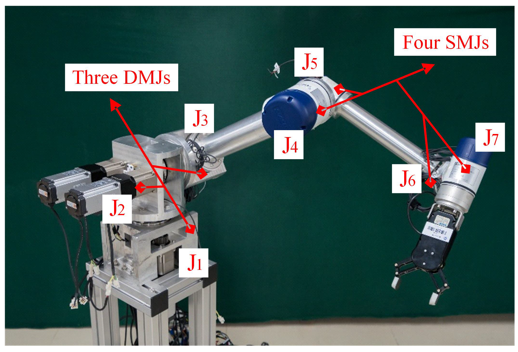
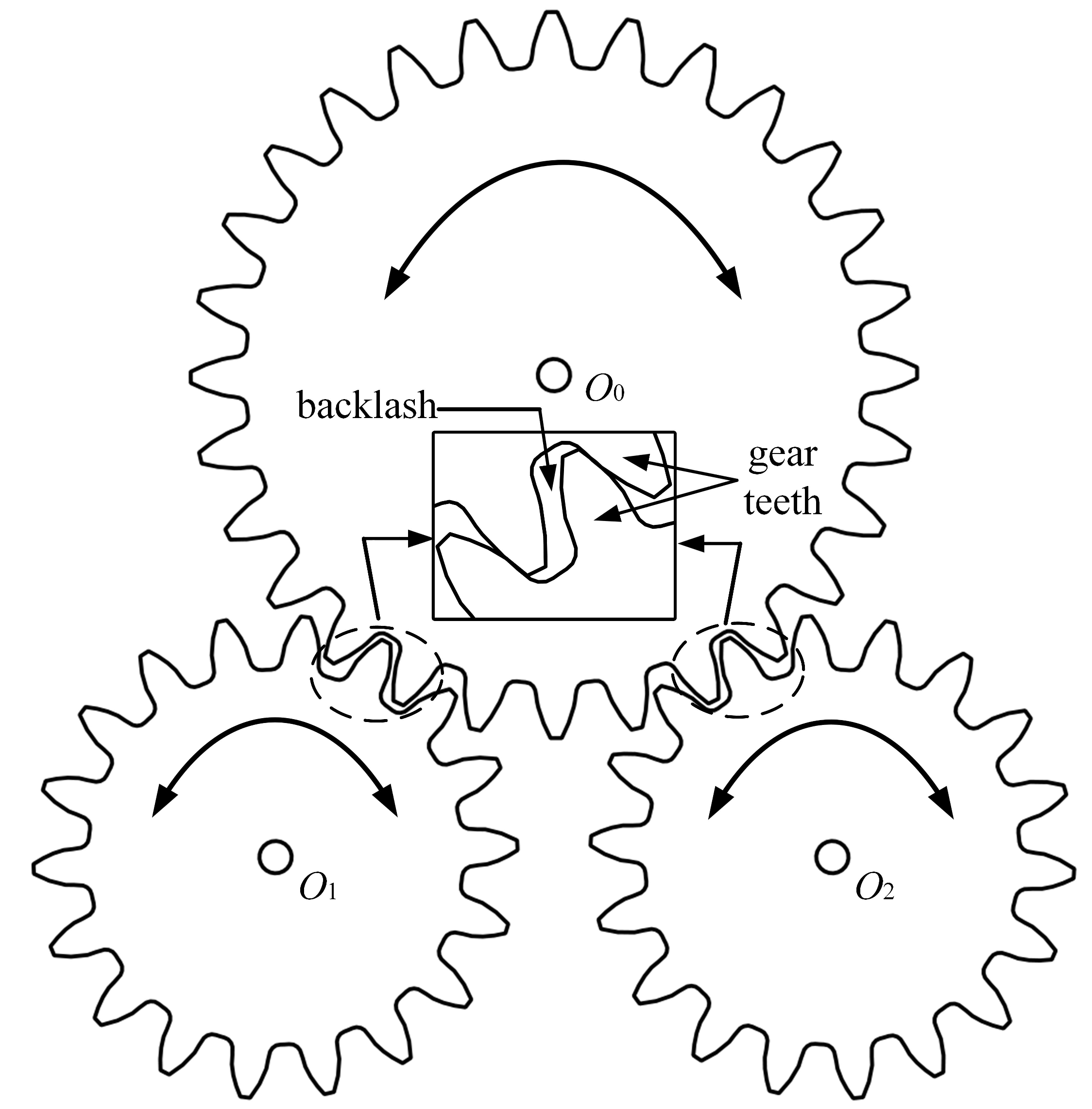
2.1. Dual-Motor Joints-Driven Robotic Manipulator and Anti-Backlash Strategy

The 7-DoF serial-type robot (named D-Arm) is depicted in Figure 2. This manipulator is composed of three dual-motor joints (DMJs, labeled as ${\mathrm{J}}_1$ to ${\mathrm{J}}_3$) and four single-motor joints (SMJs, labeled as ${\mathrm{J}}_4$ to ${\mathrm{J}}_7$). The DMJs, positioned near the base, are instrumental in enhancing the accuracy, payload capacity, and reliability of the robotic system. Conversely, the SMJs, characterized by a high torque-to-weight ratio, are strategically employed to address the challenges posed by gravitational and inertial forces near the end-effector. Further insights into the design and capabilities of this robotic system are elaborated in [10].

Remark 1.

Obviously, the D-Arm is a type of hybrid single/dual-motor joint-driven robotic manipulator. A single-motor joint can be considered a special case of a dual-motor joint, where one of the motors is always in a deactivated state. Therefore, the position tracking controller proposed in the next section of this paper are applicable to both single/motor joints. However, this work focuses on the position tracking control problem of a dual-motor joint-driven robotic manipulator. For the sake of illustration and understanding, it is assumed that the D-Arm consists of only dual-motor joints.

Figure 3 illustrates the schematic diagram of the dual-motor joint. In this configuration, $O_1$ and $O_2$ denote the two pinions that are coupled to the respective two driving motors, while $O_0$ indicates the load gear that is connected to the driven load. By applying an appropriate electrically preload to the dual-motor assembly, the joint is capable of operating without backlash. In [10], we introduced an innovative APDMAB strategy which is adept at effectively mitigating backlash, even in the presence of disturbances, without requiring prior knowledge of the backlash characteristics. In this strategy, both motors work in semi-closed-loop position control mode, and one motor is defined as primary motor while another is auxiliary motor. In order to be easily distinguished and understood, the superscript {•}* is defined as the variable related to the auxiliary motor. The essence of this strategy is that the auxiliary motor continuously adjusts the tracking trajectory to eliminate the backlash. To realize this strategy, we define the force control (FC) mode and position control (PC) mode according to the different operating states of the dual-motor as well as the desired velocity.

The FC mode ${\mathcal{S}}_{FC}\in {\mathbb{R}}^{n\times 1}$ is given by the following set

$${\mathcal{S}}_{F{C}_1}=\{(\tau ,{\tau }^{*},{\dot{q}}_d)\in {\mathbb{R}}^{n\times 3}\mid ({\dot{q}}_d\ge 0)\wedge ((\tau >{\tau }_u)\vee ({\tau }^{*}>-{\tau }_l))\}$$

(1)

$${\mathcal{S}}_{F{C}_2}=\{(\tau ,{\tau }^{*},{\dot{q}}_d)\in {\mathbb{R}}^{n\times 3}\mid ({\dot{q}}_d<0)\wedge ((\tau <{\tau }_l)\vee ({\tau }^{*}<-{\tau }_u))\}$$

(2)

$${\mathcal{S}}_{FC}={\mathcal{S}}_{F{C}_1}\cup {\mathcal{S}}_{F{C}_2}$$

(3)

where the superscript n represents the number of primary motors or the DoF of dual-motor joint-driven robotic manipulator; $\tau \in {\mathbb{R}}^{n\times 1}$, ${\tau }^{*}\in {\mathbb{R}}^{n\times 1}$, ${\dot{q}}_d\in {\mathbb{R}}^{n\times 1}$ are the control torque of primary motor, the output torque of auxiliary motor and the desired velocity of primary motor, respectively; ${\tau }_l\in {\mathbb{R}}_{+}^{n\times 1},{\tau }_u\in {\mathbb{R}}_{+}^{n\times 1}$ are lower and upper threshold torque, respectively, and ${\tau }_u>0.1{\tau }_{rat}>{\tau }_l$. Here, ${\tau }_{rat}\in {\mathbb{R}}^{n\times 1}$ represents the rated torque of motor. At $t_k$ sampling time, according to the admittance control strategy, the auxiliary motor adjusts its tracking trajectory and thus its output torque as follows

$$q_a\left(t_k\right)=q_d^{*}-q^{*}+T_s{L}^{-1}[{\tau }_h-{\tau }_c-H(q_d^{*}-q^{*})]$$

(4)

$${\tau }_h=\left\{\begin{array}{c}-0.1{\tau }_{rat}\begin{array}{cc}& \mathrm{if}{\dot{q}}_d⩾0\end{array}\hfill \\ 0.1{\tau }_{rat}\begin{array}{cc}& \mathrm{if}{\dot{q}}_d<0\end{array}\hfill \end{array}\right.{\tau }_c=\left\{\begin{array}{c}\tau \begin{array}{cc}& \mathrm{if}{\dot{q}}_d⩾0\end{array}\hfill \\ {\tau }^{*}\begin{array}{cc}& \mathrm{if}{\dot{q}}_d<0\end{array}\hfill \end{array}\right.$$

(5)

where $q_a\left(t_k\right)\in {\mathbb{R}}^{n\times 1}$ is the adjusted value at $t_k$ sampling time; $q_d^{*}\in {\mathbb{R}}^{n\times 1}$, $q^{*}\in {\mathbb{R}}^{n\times 1}$ are the desired trajectory and current position of the auxiliary motor, respectively; $T_s$ is the sampling interval; $L=diag\{l_1,l_2,\dots ,l_n\}$ and $H=diag\{h_1,h_2,\dots ,h_n\}$ are the desired damping and stiffness coefficient matrix, respectively.

In the PC mode, the compensation for the auxiliary motor is not updated to resist external disturbances. Since there are only two modes within the system, the PC mode ${\mathcal{S}}_{PC}$ is defined as the complement of the FC mode as follows

$${\mathcal{S}}_{PC}={\complement }_{{\mathbb{R}}^{n\times 3}}{\mathcal{S}}_{FC}$$

(6)

Ultimately, different compensations are applied to the reference position of the auxiliary motor depending on the different motion states of the system

$$q_a^{*}\left(t_{k+1}\right)=\left\{\begin{array}{cc}{q}_a^{*}\left(t_k\right)+q_a\left(t_k\right)\hfill & \mathrm{if}(\tau ,{\tau }^{*},{\dot{q}}_d)\in {\mathcal{S}}_{FC}\hfill \\ q_a^{*}\left(t_k\right)\hfill & \mathrm{if}(\tau ,{\tau }^{*},{\dot{q}}_d)\in {\mathcal{S}}_{PC}\hfill \end{array}\right.$$

(7)

$$q_d^{*}\left(t_{k+1}\right)=q_d\left(t_{k+1}\right)+q_a^{*}\left(t_{k+1}\right)$$

(8)

where $q_d^{*}\left(t_{k+1}\right)\in {\mathbb{R}}^{n\times 1}$ is reference position of the auxiliary motor at $t_{k+1}$.

Remark 2.

As shown in Figure 1, the output of the anti-backlash strategy only applies to the position tracking command of the auxiliary motor. The conclusion is drawn that the proposed dual-motor anti-backlash control strategy acts directly on the reference position trajectory and in such a way that only one motor provides the driving torque while the other motor provides the preloading torque. This ensures the complete decoupling of the anti-backlash control and the trajectory tracking control. Therefore, in the following robot modeling and trajectory tracking controller design, we simplify the dual-motor drive system to a single-motor drive system. In other words, the position controllers for each motor in the dual-motor joint have the same structure and parameters and all the subsequent derivations could be applied to each motor of dual-motor joint in the following content. For the sake of illustration and understanding, we will take the symbols of primary motor as an example to complete the design of the position tracking controller of the robotic manipulator.

2.2. System Model and Preliminaries

Once the non-differentiable nonlinearity in the drive train, i.e., the backlash, has been successfully eliminated, the dynamics model of backlash-free robotic systems considering uncertainties and disturbances can be given as follows [31]

$$(M_0\left(q\right)+\Delta M\left(q\right))\ddot{q}+C(q,\dot{q})\dot{q}+G\left(q\right)=\tau +{\tau }_d+{\tau }_f$$

(9)

where $q\in {\mathbb{R}}^{n\times 1}$, $\dot{q}\in {\mathbb{R}}^{n\times 1}$, $\ddot{q}\in {\mathbb{R}}^{n\times 1}$ denote the vectors of joint position, velocity, and acceleration, respectively; $M_0\left(q\right)\in {\mathbb{R}}^{n\times n}$ represents the nominal inertia matrix with $\Delta M\left(q\right)\in {\mathbb{R}}^{n\times n}$ being the uncertain section of inertia matrix; $C(q,\dot{q})\in {\mathbb{R}}^{n\times n}$ indicates the unknown centripetal Coriolis matrix; $G\left(q\right)\in {\mathbb{R}}^{n\times 1}$ represents the unknown gravity; $\tau$ is the vector of joint torque; ${\tau }_d\in {\mathbb{R}}^{n\times 1}$ is the vector associated with disturbances, and ${\tau }_f\in {\mathbb{R}}^{n\times 1}$ denotes the vector of the nonlinear joint friction.

From Equation (9), the dynamics model of backlash-free robotic systems can be simplified as

$$\ddot{q}=M_0^{-1}\left(q\right)\tau +\Phi (q,\dot{q},\ddot{q})$$

(10)

where the lumped uncertainty $\Phi (q,\dot{q},\ddot{q})$ is estimated by the proposed adaptive observer

$$\Phi (q,\dot{q},\ddot{q})=M_0^{-1}\left(q\right)(-\Delta M\left(q\right)\ddot{q}-C(q,\dot{q})\dot{q}-G\left(q\right)+{\tau }_d+{\tau }_f).$$

(11)

Assumption 1

([32]). The derivative of lumped uncertainties $\Phi (q,\dot{q},\ddot{q})$ are assumed to be unknown but bounded by the following condition

$$∥\dot{\Phi }(q,\dot{q},\ddot{q})∥\le \Pi {(q,\dot{q})}^{\mathrm{T}}b$$

(12)

where $\Pi (q,\dot{q})={\left[1,{∥\dot{q}∥}^2,cos∥\dot{q}∥\right]}^{\mathrm{T}}$ with unknown vector $b={\left[b_1,b_2,b_3\right]}^{\mathrm{T}}$.

Lemma 1

([9]). Suppose that there exists a Lyapunov function $V\left(x\right)$ with initial value of $V\left(0\right)$, and $V\left(x\right)$ satisfies the following differential inequality

$$\dot{V}\left(x\right)\le -{\rho }_{1}V\left(x\right)-{\rho }_2{V}^{\ell }\left(x\right){\rho }_1,{\rho }_2>0,0<\ell <1$$

(13)

Then the setting time T for Equation (13) is given by

$$T\le {\displaystyle \frac{1}{{\rho }_1(1-\ell )}}ln\left({\displaystyle \frac{{\rho }_1{V}^{1-\ell }\left(0\right)+{\rho }_2}{{\rho }_2}}\right)$$

(14)

Definition 1.

$si{g}^l\left(x\right)={\left|x\right|}^l\mathrm{sgn}\left(x\right)$, where $l>0$ and $\mathrm{sgn}\left(x\right)$ is the sign function.

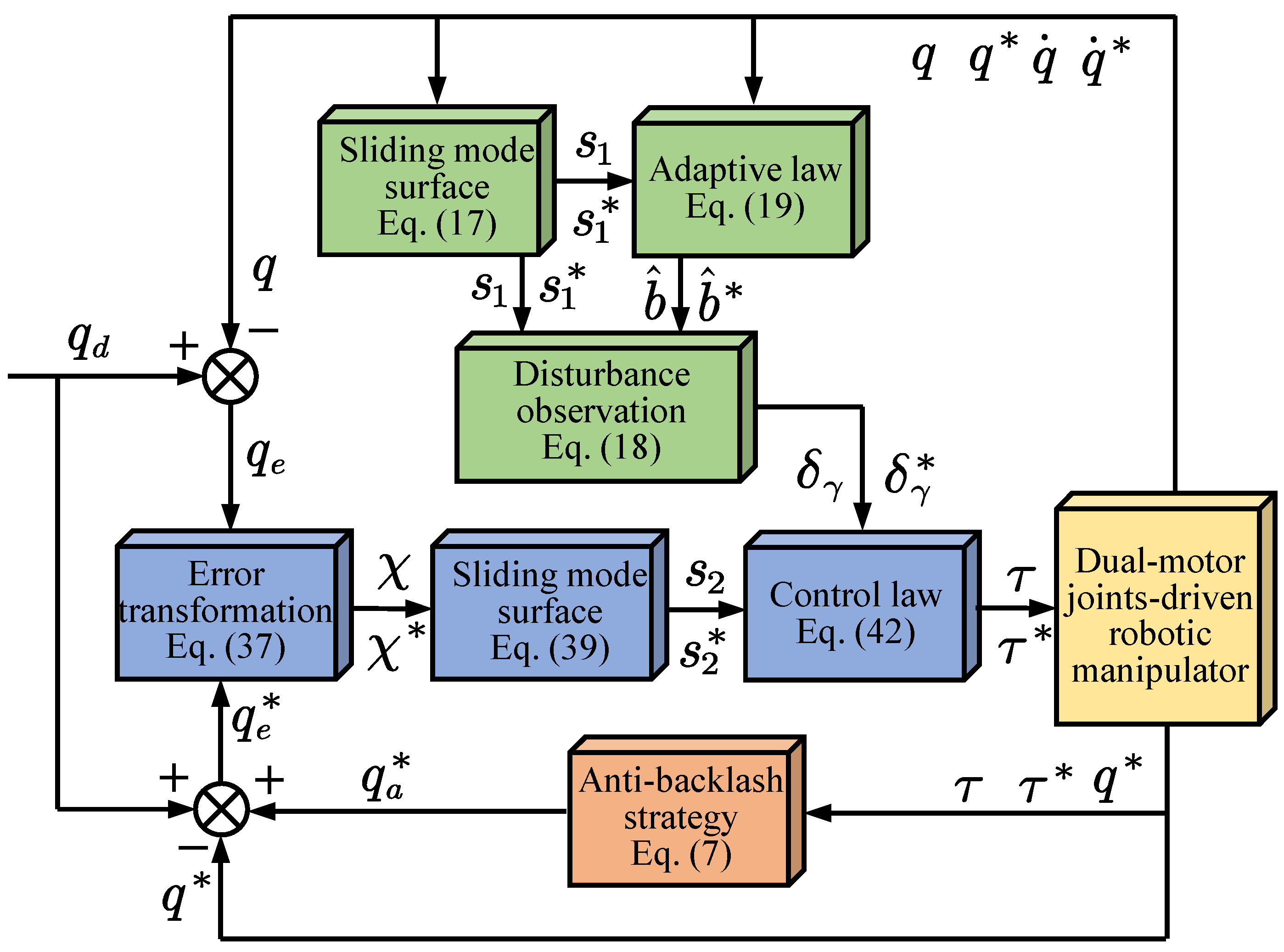
3. Observer-Based Finite-Time Tracking Control for Backlash-Free Robotic Systems

3.1. Design of Adaptive Sliding Mode Observer

Define the input discrepancy of the proposed observer as

$$z=\gamma -\dot{q}$$

(15)

where the variable $\gamma$ satisfies the following dynamic system

$$\dot{\gamma }=M_0^{-1}\left(q\right)\tau -{\eta }_{1}z-{\eta }_{2}si{g}^{\alpha }\left(z\right)+{\delta }_{\gamma }$$

(16)

where ${\eta }_1$ and ${\eta }_2$ are positive constants, $0<\alpha <1$, and the auxiliary variable ${\delta }_{\gamma }$ is designed to estimate the lumped uncertainties $\Phi (q,\dot{q},\ddot{q})$ of the closed system.

A finite time non-singular TSM surface is proposed as

$$s_1=\dot{z}+{\eta }_{1}z+{\eta }_{2}si{g}^{\alpha }\left(z\right)$$

(17)

Based on the Assumption 1, the dynamic equation of ${\delta }_{\gamma }$ can be designed as follows

$$\left\{\begin{array}{c}{\dot{\delta }}_{\gamma }=-(\Pi {(q,\dot{q})}^{\mathrm{T}}\widehat{b}+c)\mathrm{sgn}\left(s_1\right)\hfill \\ {\delta }_{\gamma }\left(0\right)=0\hfill \end{array}\right.$$

(18)

where c is a positive constant, $\widehat{b}={[{\widehat{b}}_1,{\widehat{b}}_2,{\widehat{b}}_3]}^{\mathrm{T}}$, and $\widehat{b}$ is the estimate of b in Assumption 1. An adaptive law for $\widehat{b}$ is designed as

$$\dot{\widehat{b}}=\left\{\begin{array}{cc}0,\hfill & ∥s_1∥\le \vartheta \hfill \\ -\lambda \widehat{b}+\Pi (q,\dot{q})∥s_1∥,\hfill & ∥s_1∥>\vartheta \hfill \end{array}\right.$$

(19)

where $\vartheta >0$ denotes the size of dead-zone and $\lambda >0$.

Theorem 1.

Considering the sliding mode surface Equation (17), if the auxiliary variable ${\delta }_{\gamma }$ satisfies the Equation (16), the adaptive sliding mode disturbance observer will achieve practical finite-time stability.

Proof of Theorem 1.

Considering Equations (15) and (16), the derivative of z is

$$\dot{z}=\dot{\gamma }-\ddot{q}=M_0^{-1}\left(q\right)\tau -{\eta }_{1}z-{\eta }_{2}si{g}^{\alpha }\left(z\right)+{\delta }_{\gamma }-\ddot{q}$$

(20)

Substituting Equation (10) into Equation (20), the following is obtained

$$\dot{z}=-{\eta }_{1}z-{\eta }_{2}si{g}^{\alpha }\left(z\right)+{\delta }_{\gamma }-\Phi (q,\dot{q},\ddot{q})$$

(21)

Combine Equations (17) and (21), we can obtain that

$$s_1={\delta }_{\gamma }-\Phi (q,\dot{q},\ddot{q})$$

(22)

According to Equation (18), ${\dot{s}}_1$ can be given as

$$\begin{array}{c}{\dot{s}}_1={\dot{\delta }}_{\gamma }-\dot{\Phi }(q,\dot{q},\ddot{q})\hfill \\ =-(\Pi {(q,\dot{q})}^{\mathrm{T}}\widehat{b}+c)\mathrm{sgn}\left(s_1\right)-\dot{\Phi }(q,\dot{q},\ddot{q})\hfill \end{array}$$

(23)

Define $\tilde{b}=b-\widehat{b}$. We choose the Lyapunov function as

$$V_1={\displaystyle \frac{1}{2}}{s}_1^{\mathrm{T}}{s}_1+{\displaystyle \frac{1}{2}}{\tilde{b}}^{\mathrm{T}}\tilde{b}$$

(24)

Insert the adaptive law Equation (19), ${\dot{V}}_1$ can be derived as

$$\begin{array}{c}{\dot{V}}_1={s_1}^{\mathrm{T}}\left[-\left(\Pi {(q,\dot{q})}^{\mathrm{T}}\widehat{b}+c\right)\mathrm{sgn}\left(s_1\right)-\dot{\Phi }(q,\dot{q},\ddot{q})\right]-\Pi {(q,\dot{q})}^{\mathrm{T}}∥s_1∥\tilde{b}+\lambda {\tilde{b}}^{\mathrm{T}}\widehat{b}\hfill \\ \le -c∥s_1∥-\left[\Pi {(q,\dot{q})}^{\mathrm{T}}b-∥\dot{\Phi }(q,\dot{q},\ddot{q})∥\right]∥s_1∥+\lambda {\tilde{b}}^{\mathrm{T}}\widehat{b}\hfill \end{array}$$

(25)

Denote ${\varpi }_1=c+\left(\Pi {(q,\dot{q})}^{\mathrm{T}}b-∥\dot{\Phi }(q,\dot{q},\ddot{q})∥\right)$, According to the proof in the existing work [33], it yields

$$\begin{array}{c}{\dot{V}}_1\le -min\left\{{\varpi }_1,1\right\}\left(∥s_1∥+∥\tilde{b}∥\right)+({∥\tilde{b}∥}^2{)}^{{\displaystyle \frac{1}{2}}}+\lambda {\tilde{b}}^{\mathrm{T}}\widehat{b}\hfill \\ \le -\sqrt{2}min\left\{{\varpi }_1,1\right\}{V}_1^{{\displaystyle \frac{1}{2}}}+({∥\tilde{b}∥}^2{)}^{{\displaystyle \frac{1}{2}}}+\lambda {\tilde{b}}^{\mathrm{T}}\widehat{b}\hfill \end{array}$$

(26)

Note that the following inequality holds

$$\begin{array}{c}({∥\tilde{b}∥}^2{)}^{{\displaystyle \frac{1}{2}}}+\lambda {\tilde{b}}^{\mathrm{T}}\widehat{b}=({∥\tilde{b}∥}^2{)}^{{\displaystyle \frac{1}{2}}}+\lambda {\tilde{b}}^{\mathrm{T}}(b-\tilde{b})\hfill \\ \le ({∥\tilde{b}∥}^2{)}^{{\displaystyle \frac{1}{2}}}+{\displaystyle \frac{\lambda }{2}}({∥b∥}^2-{∥\tilde{b}∥}^2)\hfill \\ \le {\displaystyle \frac{1}{2\lambda }}+{\displaystyle \frac{\lambda }{2}}{∥b∥}^2\hfill \end{array}$$

(27)

From inequality Equation (26), one can obtain

$${\dot{V}}_1\le -\sqrt{2}min\left\{{\varpi }_1,1\right\}{V_1}^{{\displaystyle \frac{1}{2}}}+{\varpi }_2$$

(28)

where ${\varpi }_2={\displaystyle \frac{1}{2\lambda }}+{\displaystyle \frac{\lambda }{2}}{∥b∥}^2$.

According to the analyses in the existing works [33,34], the variables $s_1$ and $\tilde{b}$ are bounded. In addition, we can obtain the bounded set ${\mathcal{S}}_{s_1}=\left\{s_1\in {\mathbb{R}}^{n\times 1}\left|∥s_1∥\le {\Delta }_{s_1}\right.\right\}$ with ${\Delta }_{s_1}={\displaystyle \frac{{\varpi }_2}{(1-{\theta }_0)min\left\{{\varpi }_1,1\right\}}}$ and $0<{\theta }_0<1$, and $s_1$ will be driven into the bounded set ${\mathcal{S}}_{s_1}$ in finite time. It can be noted that the variable z and $\dot{z}$ are also bounded, since $s_1$ is bounded.

Next, the convergence region of z and $\dot{z}$ will be discussed in the following content.

As the $s_1$ reach the bounded set ${\mathcal{S}}_{s_1}$, we can get

$$\Omega =\dot{z}+{\eta }_{1}z+{\eta }_{2}si{g}^{\alpha }\left(z\right),∥\Omega ∥\le {\Delta }_{s_1}$$

(29)

We choose the Lyapunov function as

$$V_2={\displaystyle \frac{1}{2}}{z}^{\mathrm{T}}z$$

(30)

The Lyapunov function Equation (30) is derived as

$$\begin{array}{c}{\dot{V}}_2=z^{\mathrm{T}}\dot{z}\hfill \\ =z^{\mathrm{T}}\left(\Omega -{\eta }_{1}z-{\eta }_{2}si{g}^{\alpha }\left(z\right)\right)\hfill \\ \le -{\eta }_1{∥z∥}^2-{\eta }_2{∥z∥}^{1+\alpha }+z^{\mathrm{T}}\Omega \hfill \\ \le -2{\eta }_1{V}_2-2{\eta }_2{V_2}^{{\displaystyle \frac{1+\alpha }{2}}}+∥z∥{\Delta }_{s_1}\hfill \end{array}$$

(31)

Equation (31) can be rearranged into the following two forms

$${\dot{V}}_2\le -2\left({\eta }_1-{\displaystyle \frac{{\Delta }_{s_1}}{2∥z∥}}\right)V_2-2{\eta }_2{V_2}^{{\displaystyle \frac{1+\alpha }{2}}}$$

(32)

$${\dot{V}}_2\le -2{\eta }_1{V}_2-2\left({\eta }_2-{\displaystyle \frac{{\Delta }_{s_1}}{2{∥z∥}^{\alpha }}}\right)V_2^{{\displaystyle \frac{1+\alpha }{2}}}$$

(33)

From Lemma 1, if ${\eta }_1-{\displaystyle \frac{{\Delta }_{s_1}}{2∥z∥}}>0$ in Equation (32), the error z will converge to the bound $∥z∥\le {\displaystyle \frac{{\Delta }_{s_1}}{2{\eta }_1}}$ in finite time. Similarly, if ${\eta }_2-{\displaystyle \frac{{\Delta }_{s_1}}{2{∥z∥}^{\alpha }}}>0$ in Equation (33), the error z will converge to the bound $∥z∥\le \sqrt[\alpha ]{{\displaystyle \frac{{\Delta }_{s_1}}{2{\eta }_2}}}$.

Thus, z will ultimately converge to the bound

$$∥z∥\le {\Delta }_z=min\left\{{\displaystyle \frac{{\Delta }_{s_1}}{2{\eta }_1}},\sqrt[\alpha ]{{\displaystyle \frac{{\Delta }_{s_1}}{2{\eta }_2}}}\right\}$$

(34)

From Equation (29), the bound of $\dot{z}$ is

$$∥\dot{z}∥\le {\Delta }_{\dot{z}}={\Delta }_{s_1}+{\eta }_1{\Delta }_z+{\eta }_2{\Delta }_z^{\alpha }$$

(35)

Then, based on the above analysis, we can conclude that the variable z and $\dot{z}$ are all bounded. The observer could achieve practical finite-time stability. The proof is completed.    □

Remark 3.

In practice, the lumped uncertainties $\Phi (q,\dot{q},\ddot{q})$ is subject to high variability and is dependent on the position q and velocity $\dot{q}$ and acceleration $\ddot{q}$. Consequently, obtaining precise prior knowledge of the upper bounds of $\Phi (q,\dot{q},\ddot{q})$ and its derivative $\dot{\Phi }(q,\dot{q},\ddot{q})$ is challenging. Existing sliding mode controllers, such as those works in [31,35], typically assume that the derivative of the lumped uncertainties is bounded by known positive constants. In contrast, the adaptive sliding mode disturbance observer (ASMDO) proposed here is designed to estimate these lumped uncertainties, thereby alleviating the need for such prior knowledge. The ASMDO ensures that the estimation error achieves finite-time convergence, characterized by $∥\Phi (q,\dot{q},\ddot{q})-{\delta }_{\gamma }∥={\delta }_e$. Hence, there must exist a positive constant ${\beta }_{\gamma }$ that satisfies ${\beta }_{\gamma }\ge ∥{\delta }_e∥$. It indicates a robust performance against the lumped uncertainties.

3.2. Design of Prescribed Performance Sliding Mode Controller

To enhance the control performance of the system, a prescribed performance function (PPF) is incorporated into the controller, ensuring that the tracking error remains strictly within a predefined domain. The PPF is mathematically described as follows

$$\rho \left(t\right)=({\mu }_0-{\mu }_{\infty })exp(-at)+{\mu }_{\infty }$$

(36)

where $a>0$ and ${\mu }_0>{\mu }_{\infty }>0$. Define $q_{ei}(i=1,2,\dots ,n)$ as the i-th element of tracking error and satisfy the inequality $-{\epsilon }_i\rho \left(t\right)<q_{ei}<{\epsilon }_i\rho \left(t\right),0<{\epsilon }_i\le 1$. Consider the following error transformation

$${\chi }_i={\displaystyle \frac{1}{2}}ln\left({\displaystyle \frac{\frac{q_{ei}}{\rho \left(t\right)}+{\epsilon }_i}{{\epsilon }_i-\frac{q_{ei}}{\rho \left(t\right)}}}\right)$$

(37)

where ${\chi }_i$ denotes the i-th element of transformed error, and $\chi ={[{\chi }_1,{\chi }_2,\dots ,{\chi }_n]}^{\mathrm{T}}$.

Define $\psi =diag\{{\psi }_1,{\psi }_2,\dots ,{\psi }_n\}$ with ${\psi }_i={\displaystyle \frac{{\epsilon }_i}{\left({\epsilon }_i\rho \left(t\right)+q_{e\mathrm{i}}\right)\left({\epsilon }_i\rho \left(t\right)-q_{ei}\right)}}$. Based on Equations (36) and (37), the dynamic equation of transformed error is

$$\begin{array}{c}\dot{\chi }=\psi (\Theta {\dot{q}}_e-\dot{\Theta }{q}_e)\hfill \\ \ddot{\chi }=\psi \Theta \left(M_0^{-1}\left(q\right)\tau +\Phi (q,\dot{q},\ddot{q})-{\ddot{q}}_d\right)+\Xi \hfill \end{array}$$

(38)

where $\Theta =diag\{{\rho }_1\left(t\right),{\rho }_2\left(t\right),\dots ,{\rho }_n\left(t\right)\}$ and $\Xi =\dot{\psi }(\Theta {\dot{q}}_e-\dot{\Theta }{q}_e)-\psi \ddot{\Theta }{q}_e$.

Considering the singularity-free fast convergence, a novel finite-time sliding mode surface based on the transformed error is designed as follows

$$s_2=\chi +{\zeta }_{1}si{g}^{1/\phantom{1\upsilon }\upsilon }(\dot{\chi }+{\zeta }_2\chi )$$

(39)

where ${\zeta }_1,{\zeta }_2>0$ and $0<\upsilon <1$.

Take the time derivative of $s_2$ as

$${\dot{s}}_2=\dot{\chi }+{\displaystyle \frac{{\zeta }_1}{\upsilon }}{\left|\dot{\chi }+{\zeta }_2\chi \right|}^{1/\phantom{1\upsilon }\upsilon -1}(\ddot{\chi }+{\zeta }_2\dot{\chi })$$

(40)

In order to guarantee fast convergence and good trajectory tracking performance for the closed-loop control system, inspired by [36], a faster TSM-type reaching law is proposed as

$${\dot{s}}_2=-{\displaystyle \frac{1}{R\left(s_2\right)}}\left({\gamma }_1{s}_2+{\gamma }_{2}si{g}^{\beta }\left(s_2\right)\right)$$

(41)

where $R\left(s_2\right)=x_1+(1-x_1)exp(-y_1{∥s_2∥}^{z_1})$, $0<x_1<1$, $y_1>0$, $z_1$ is an even integer. $0<\beta <1$, ${\gamma }_1$ and ${\gamma }_2$ are positive constants.

Remark 4.

It is evident that $R\left(s_2\right)$ is strictly positive, indicating that it does not influence the stabilization of the control system. Given that the initial state of $s_2$ is significantly distant from the equilibrium point, $1/R\left(s_2\right)$ tends to $1/x_1>1$, thereby potentially accelerating the convergence rate during the transient phase. In contrast, when the state of $s_2$ approaches to equilibrium point, $R\left(s_2\right)$ tends to 1. This means that $R\left(s_2\right)$ could be utilized to tune the convergence rate.

Based on the dynamics Equation (40), the NFTSMC control law can be defined as

$$\tau =M_0\left(q\right)\left(-{\delta }_{\gamma }+{\ddot{q}}_d\right)-M_0\left(q\right){\psi }^{-1}{\Theta }^{-1}\left(-{\beta }_{\gamma }\mathrm{sgn}\left(s_1\right)+\Xi +{\zeta }_2\dot{\chi }-f(\chi ,\dot{\chi })+{\displaystyle \frac{{\gamma }_1{s}_2+{\gamma }_{2}si{g}^{\beta }\left(s_2\right)}{R\left(s_2\right)}}\right)$$

(42)

where ${\beta }_{\gamma }\mathrm{sgn}\left(s_1\right)$ is the robustness term for the observer error. Moreover, in order to simplify the calculation, the auxiliary function is proposed by $f(\chi ,\dot{\chi })={\displaystyle \frac{\upsilon }{{\zeta }_1}}si{g}^{2-1/\phantom{1\upsilon }\upsilon }(\dot{\chi }+{\zeta }_2\chi )+{\zeta }_2(\dot{\chi }+{\zeta }_2\chi )$.

Theorem 2.

Considering the sliding mode surface defined by Equation (39) and the control law given by Equation (42), if the adaptive sliding mode disturbance observer satisfied with finite-time stability, the closed-loop control system is guaranteed to achieve stabilization within a finite-time $T_c$.

Proof of Theorem 2.

Choose the Lyapunov function as $V_2=0.5s_2^{\mathrm{T}}{s}_2$ and let $u=\dot{\chi }+{\zeta }_2\chi$, then take the time derivative of $V_2$ as

$${\dot{V}}_2=s_2^{\mathrm{T}}\left[\dot{\chi }+{\displaystyle \frac{{\zeta }_1}{\upsilon }}{\left|u\right|}^{1/\phantom{1\upsilon }\upsilon -1}\left(\psi \Theta \left(M_0^{-1}\left(q\right)\tau +\Phi (q,\dot{q},\ddot{q})-{\ddot{q}}_d\right)+\Xi +{\zeta }_2\dot{\chi }\right)\right]$$

(43)

Substituting Equation (42) into Equation (43), we have

$${\dot{V}}_2=s_2^{\mathrm{T}}\left[-{\zeta }_2{s}_2+{\displaystyle \frac{{\zeta }_1}{\upsilon }}{\left|u\right|}^{1/\phantom{1\upsilon }\upsilon -1}\left(\Phi (q,\dot{q},\ddot{q})-{\delta }_{\gamma }-{\beta }_{\gamma }\mathrm{sgn}\left(s_1\right)-{\displaystyle \frac{{\gamma }_1{s}_2+{\gamma }_{2}si{g}^{\beta }\left(s_2\right)}{R\left(s_2\right)}}\right)\right]$$

(44)

As the adaptive sliding mode disturbance observer achieve the finite-time stability, one has as follow

$$\begin{array}{c}{\dot{V}}_2\le s_2^{\mathrm{T}}\left[-{\zeta }_2{s}_2+{\displaystyle \frac{{\zeta }_1}{\upsilon }}{\left|u\right|}^{1/\phantom{1\upsilon }\upsilon -1}\left(-{\displaystyle \frac{1}{R\left(s_2\right)}}\left({\gamma }_1{s}_2+{\gamma }_{2}si{g}^{\beta }\left(s_2\right)\right)\right)\right]\hfill \\ \le -{\zeta }_2{s}_2^2-{\displaystyle \frac{{\gamma }_1{\zeta }_1}{R\left(s_2\right)\upsilon }}{\left|u\right|}^{1/\phantom{1\upsilon }\upsilon -1}{s}_2^2-{\displaystyle \frac{{\gamma }_2{\zeta }_1}{R\left(s_2\right)\upsilon }}{\left|u\right|}^{1/\phantom{1\upsilon }\upsilon -1}{\left|s_2\right|}^{\beta +1}\hfill \\ \le -{\omega }_1{V}_2-{\omega }_2{V}_2^{0.5(\beta +1)}\hfill \end{array}$$

(45)

where ${\omega }_1=2({\zeta }_2+{\displaystyle \frac{{\gamma }_1{\zeta }_1}{R\left(s_2\right)\upsilon }}{\left|u\right|}^{1/\phantom{1\upsilon }\upsilon -1})$, ${\omega }_2=2^{0.5(\beta +1)}{\displaystyle \frac{{\gamma }_2{\zeta }_1}{R\left(s_2\right)\upsilon }}{\left|u\right|}^{1/\phantom{1\upsilon }\upsilon -1}$.

Remark 5.

Based on the above analysis, the control law could guarantee the sliding mode surface reach $s_2=0$ in finite time $t_{c1}$ as $u\ne 0$. Then we will discuss the case of $u=0$. If $u=0$, the auxiliary function $f(\chi ,\dot{\chi })=0$ and the control law will be rewritten as $\tau =M_0\left(q\right)\left(\Pi (q,\dot{q})-{\delta }_{\gamma }+{\ddot{q}}_d\right)-M_0\left(q\right){\psi }^{-1}{\Theta }^{-1}\left(\Xi +{\zeta }_2\dot{\chi }+{\displaystyle \frac{1}{R\left(s_2\right)}}\left({\gamma }_1{s}_2+{\gamma }_{2}si{g}^{\beta }\left(s_2\right)\right)\right)$. The time derivative of u is $\dot{u}=\ddot{\chi }+{\zeta }_2\dot{\chi }$. Substituting the new form of control law into $\dot{u}$, one can get $\dot{u}=-{\displaystyle \frac{1}{R\left(s_2\right)}}\left({\gamma }_1{s}_2+{\gamma }_{2}si{g}^{\beta }\left(s_2\right)\right)$. Note that $\dot{u}<0$ for $s_2>0$ and $\dot{u}>0$ for $s_2<0$. We can conclude that u will leave the state $u=0$ quickly and get into the desired regions.

Remark 6.

To attenuate the harmful chattering problem caused by $\mathrm{sgn}\left(s\right)$, a boundary layer function $BLF\left(s\right)={\displaystyle \frac{s}{\left|s\right|+\eta }}$ can be utilized to replace $\mathrm{sgn}\left(s\right)$, where η is a sufficient small constant.

When $s_2=0$ has reached after $t_{c1}$, one has

$$\dot{\chi }=-{\displaystyle \frac{\upsilon }{{\zeta }_1}}si{g}^{\upsilon }\left(\chi \right)-{\zeta }_2\chi$$

(46)

Similarly, based on Lemma 1, the error $\chi$ could reach $\chi =0$ in finite time $t_{c2}$ which satisfied the setting time Equation (14). Consequently, the control system will stabilize in finite time, and the setting time is bounded by

$$T_c\le T_{cmax}\stackrel{\Delta }{=}{t}_{c1}+t_{c2}$$

(47)

The proof is completed.    □

Remark 7.

From a practical standpoint, the integration of NFTSMC control with PPC is highly beneficial. This approach can yield superior transient-steady-state performance for the closed-loop system. The trajectory tracking error is strictly confined within a preassigned boundary, ensuring that the maximum overshoot does not exceed ${\mu }_0$ and the steady-state error is maintained below ${\mu }_{\infty }$. Furthermore, the tracking error is capable of converging to zero within finite-time.

Figure 1 shows our control algorithm consisting of APDMAB, ASMDO, and PPC-based NFTSMC. Due to APDMAB completely decoupling the dual-motor anti-backlash control and trajectory tracking control, the dual-motor of each joint have identical position control structures and parameters. The practical implementation details of the designed control procedure are concisely outlined in Algorithm  1.

Algorithm 1 The algorithm of the proposed controller

1: Initialization: Set dual-motor anti-backlash control parameters ${\tau }_l,{\tau }_u,L,H$, and adaptive sliding mode observer parameters $\alpha ,{\eta }_1,{\eta }_2,\zeta$, and prescribed performance function parameters $a,{\mu }_0,{\mu }_{\infty },{\epsilon }_i$, and sliding mode control parameters ${\beta }_{\gamma },\beta ,{\zeta }_1,{\zeta }_2,\upsilon ,{\gamma }_1,{\gamma }_2,x_1,y_1,z_1$; 2: Run procedure: 2.1: Compute the desired position of auxiliary motor $q_d^{*}$ from Equation (8); 2.2: Compute the sliding mode surface $s_1,s_1^{*}$ from Equation (17); 2.3: Update the adaptive law $\dot{\widehat{b}},{\dot{\widehat{b}}}^{*}$ given in Equation (19); 2.4: Compute the lumped uncertainties ${\delta }_{\gamma },{\delta }_{\gamma }^{*}$ via Equation (18); 2.5: Calculate the transformed error $\chi ,{\chi }^{*}$ from Equation (37); 2.6: Calculate the sliding mode surface $s_2,s_2^{*}$ via Equation (39); 2.7: Calculate the control law $\tau ,{\tau }^{*}$ by Equation (42) at $t_k=k{T}_s$, $k\in {\mathbb{N}}_{+}$; 2.8: Continuation: $k=k+1$; 3: End procedure

4. Simulation and Experimental Results

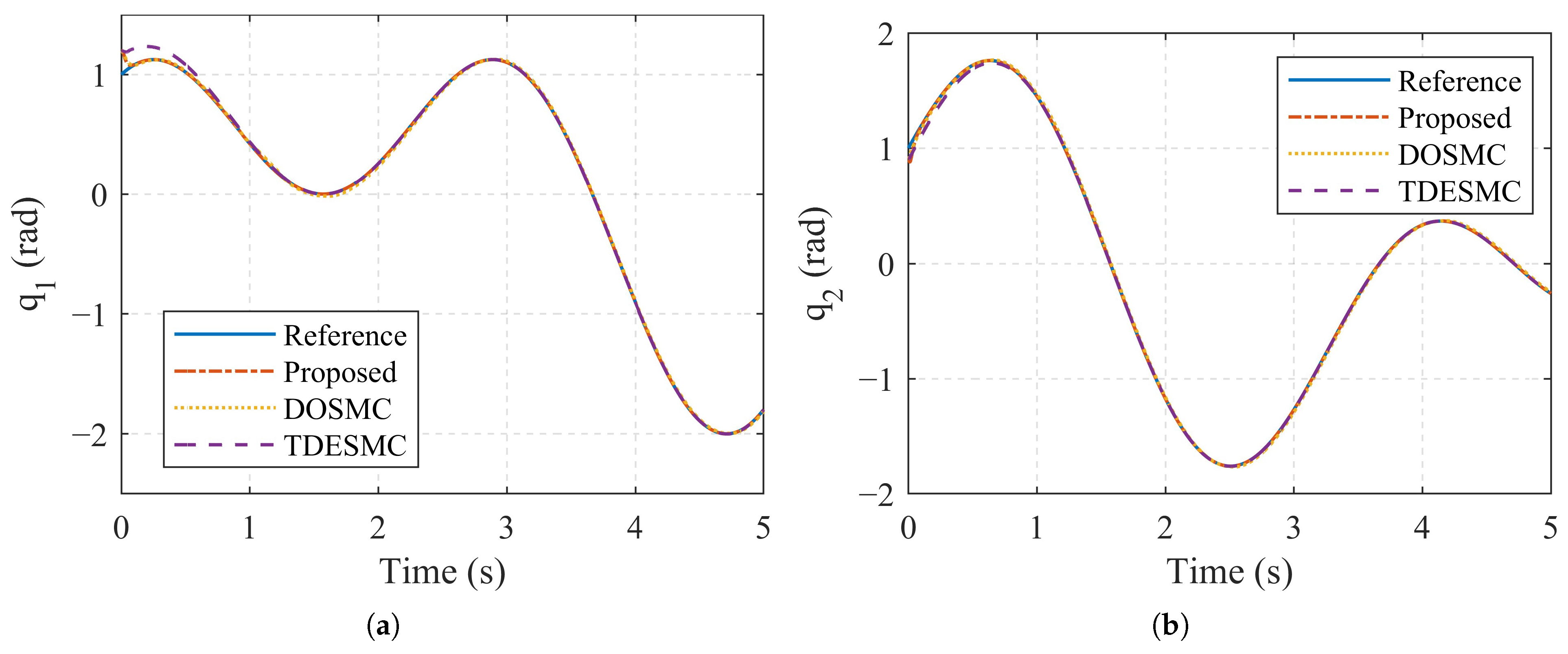
4.1. Numerical Simulation

In this section, numerical simulations for a 2-DoF robotic manipulator are presented to demonstrate the superiority and effectiveness of the proposed control scheme. The dynamics of the robotic manipulator, as characterized by Equation (9), can be articulated as follows [37]

$$\begin{array}{c}{M}_0\left(q\right)=\left[\begin{array}{cc}{p}_1+p_2+2p_{3}cos{q}_2& p_2+p_{3}cos{q}_2\\ p_2+p_{3}cos{q}_2& p_2\end{array}\right]\\ \Delta M=\left[\begin{array}{cc}{I}_{\Delta 1}+I_{\Delta 2}& I_{\Delta 2}\\ I_{\Delta 2}& I_{\Delta 2}\end{array}\right]\\ C(q,\dot{q})=\left[\begin{array}{cc}-p_3{\dot{q}}_{2}sin{q}_2& -p_3({\dot{q}}_1+{\dot{q}}_2)sin{q}_2\\ p_3{\dot{q}}_{1}sin{q}_2& 0\end{array}\right]\\ G\left(q\right)=\left[\begin{array}{c}{p}_{4}gcos{q}_1+p_{5}gcos(q_1+q_2)\\ p_{5}gcos(q_1+q_2)\end{array}\right]\end{array}$$

(48)

where $p_1=m_1{l}_{c1}^2+m_2{l}_1^2+I_{01}$, $p_2=m_2{l}_{c2}^2+I_{02}$, $p_3=m_2{l}_1{l}_{c1}$, $p_4=m_1{l}_{c2}+m_2{l}_1$, $p_5=m_2{l}_{c2}$, $l_{c1}=0.5l_1$ and $l_{c2}=0.5l_2$; A 15% model parameters perturbation in joint inertia is assumed, i.e., $I_{\Delta 1}=0.15I_{01},I_{\Delta 2}=0.15I_{02}$. The disturbances and Stribeck friction models are chosen as follows

$$\begin{array}{c}{\tau }_d\left(t\right)=\left\{\begin{array}{c}{\left[\begin{array}{c}sin\left(0.2\pi t\right)+0.15sin\left(2\pi t\right)+10,\hfill \\ 1.5sin\left(0.25\pi t\right)+4\hfill \end{array}\right]}^{\mathrm{T}},1.2\mathrm{s}>t\ge 1\mathrm{s}\hfill \\ {\left[\begin{array}{c}sin\left(0.2\pi t\right)+0.15sin\left(2\pi t\right),\hfill \\ 1.5sin\left(0.25\pi t\right)\hfill \end{array}\right]}^{\mathrm{T}},\mathrm{otherwise}\hfill \end{array}\right.\hfill \end{array}$$

(49)

$${\tau }_f\left(\dot{q}\right)=\mathrm{sgn}\left(\dot{q}\right)\left[F_c+(F_s-F_c)e^{-\left|{\displaystyle \frac{\dot{q}}{v_s}}\right|}\right]+F_v\dot{q}$$

(50)

As a result, the actual lumped uncertainties $\Phi (q,\dot{q},\ddot{q})$ can be computed by Equation (11) adopted in simulation. To ensure that the friction torque is reasonable during simulation, the Stribeck friction model parameters are referenced from [38]. The parameter values for the robot manipulator are detailed in

Table 1. Parameter values of the robotic manipulator for simulation.

Parameter	Description	Value
$l_1$	Length of first link	$0.35\mathrm{m}$
$l_2$	Length of second link	$0.32\mathrm{m}$
$m_1$	Mass of first link	$2.00\mathrm{kg}$
$m_2$	Mass of second link	$0.85\mathrm{kg}$
$I_{01}$	Inertia of first link	$61.25\times {10}^{-3}{\mathrm{kgm}}^2$
$I_{02}$	Inertia of second link	$20.42\times {10}^{-3}{\mathrm{kgm}}^2$
g	Gravitational constant	$9.8\mathrm{m}/{\mathrm{s}}^2$
$F_c$	Coulomb friction coefficient	$1.5\mathrm{Nm}$
$F_v$	viscous friction coefficient	$3.0\mathrm{Nm}$
$F_s$	Stribeck friction coefficient	$2.0\mathrm{Nm}$
$v_s$	Stribeck friction velocity	$25.0\mathrm{rad}/\mathrm{s}$

. Subsequently, the parameters pertinent to our controller design are enumerated in

Table 2. Parameter values of controller.

Section	Parameters
APDMAB	$\begin{array}{c}{\tau }_l=0.08{\tau }_{rat},{\tau }_u=0.2{\tau }_{rat},h_i=0.002,l_i=1.0\hfill \end{array}$
PPF	$\begin{array}{c}a=5,{\mu }_0=0.35,{\mu }_{\infty }=0.01,{\epsilon }_i=0.9\hfill \end{array}$
NFTSMC	$\begin{array}{c}{\beta }_{\gamma }=1.0,\beta =0.8,{\zeta }_1=1,{\zeta }_2=5,\upsilon =0.5\hfill \\ {\gamma }_1={\gamma }_2=1,x_1=0.9,y_1=5,z_1=2\hfill \end{array}$
ASMDO	$\begin{array}{c}\alpha =0.5,{\eta }_1=1,{\eta }_2=1,\lambda =0.1,c=0.05\hfill \end{array}$

.

The primary guidelines for tuning the design parameters are outlined as follows

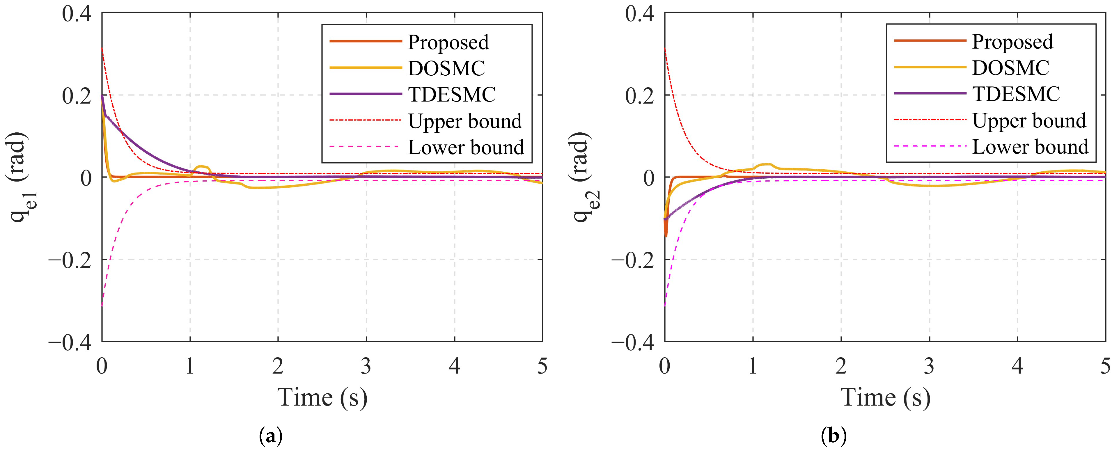
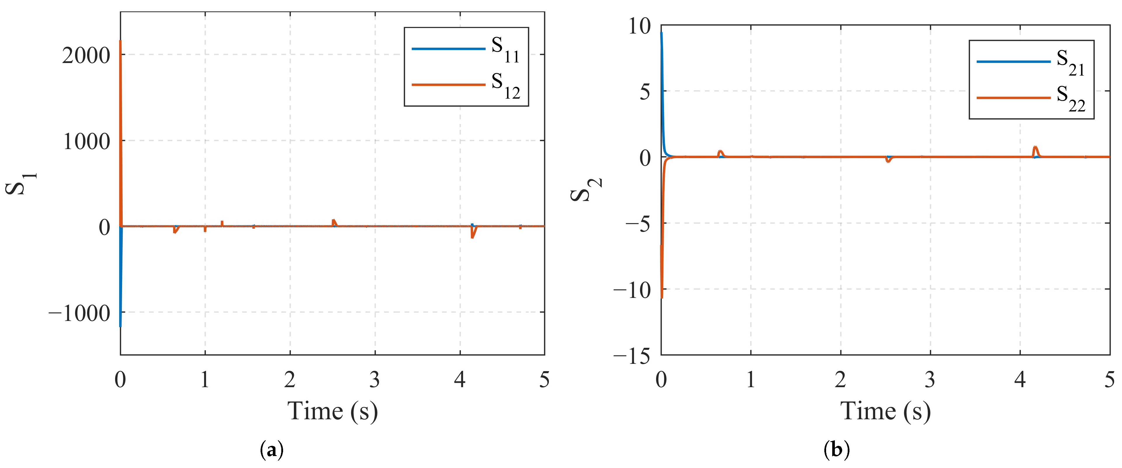
• For the sliding mode surface defined by Equation (39), the gain ${\zeta }_1$ and ${\zeta }_2$ are selected to facilitate the convergence of the sliding mode. In practical applications, an appropriately chosen ${\zeta }_2$ can enhance the convergence rate, especially when the sliding mode variable is significantly displaced from the equilibrium point. Subsequently, the designer should primarily focus on adjusting the value of ${\zeta }_1$ to optimize the system performance.
• Based on the prescribed performance function Equation (36), the initial tracking error condition $-{\epsilon }_i\rho \left(t\right)<q_{ei}<{\epsilon }_i\rho \left(t\right)$ should be fulfilled by suitable ${\mu }_0,{\mu }_{\infty }$ and a.
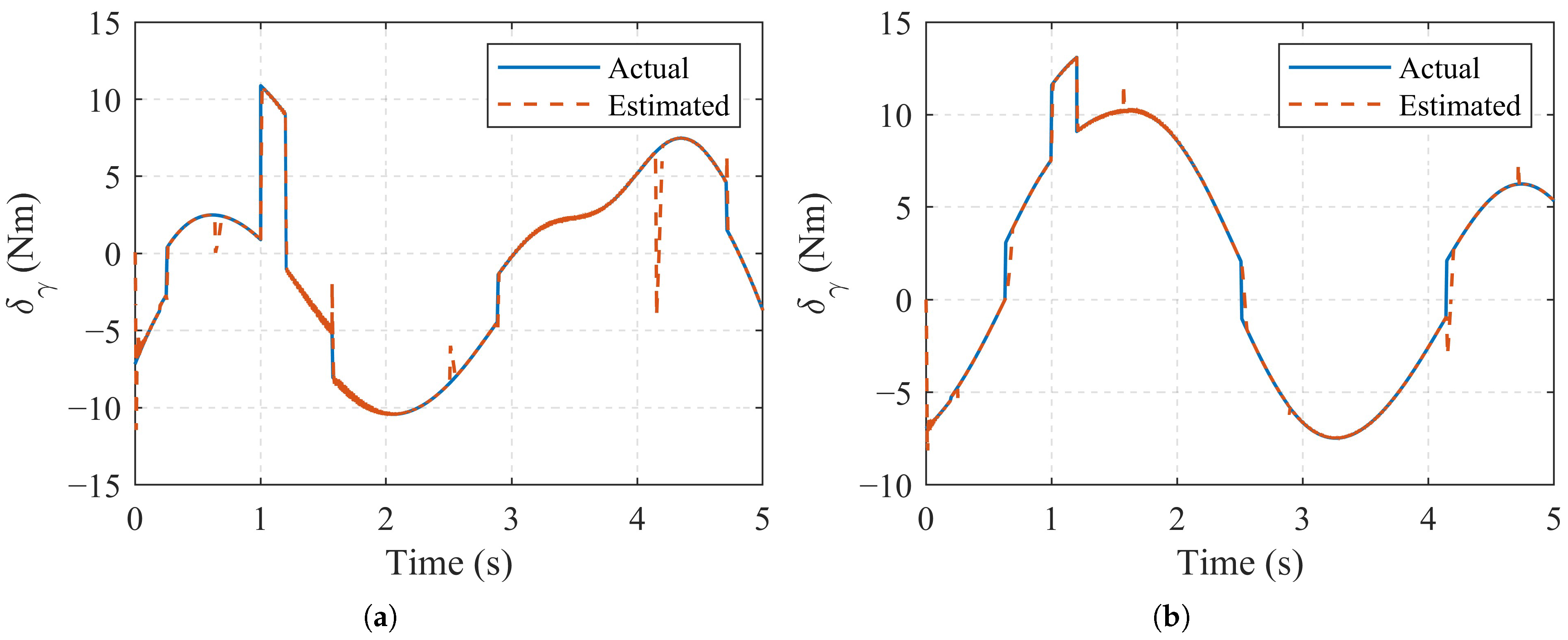
• The larger gain ${\eta }_1,{\eta }_2$ could improve the convergence rate of ASMDO. However, larger gain ${\eta }_1,{\eta }_2$ will cause large overshoot in the transient stage.
• The parameter $\upsilon ,\zeta ,{\eta }_1,{\eta }_2$ play an important roles in convergence time and accuracy for ASMDO.

The desired trajectories for the comparative study are defined as $q_{d1}\left(t\right)=sin\left(t\right)+cos\left(2t\right)$ and $q_{d2}\left(t\right)=sin\left(2t\right)+cos\left(t\right)$. The initial conditions for the robotic manipulator are specified with positions and velocities as $q_1\left(0\right)=1.2$, ${\dot{q}}_1\left(0\right)=0$, $q_2\left(0\right)=0.8$ and ${\dot{q}}_2\left(0\right)=0$. Furthermore, the joint torque limits are set to ±50 Nm.

To validate the superiority of our proposed method, a comparative simulation is conducted with two established sliding mode control (SMC) algorithms: time-delay estimation-based sliding mode control (TDESMC) [16] and disturbance observer-based sliding mode control (DOSMC) [23]. The comparative outcomes in terms of trajectory tracking profiles and tracking errors are depicted in Figure 4 and Figure 5, respectively. It is evident that the transient-state response of TDESMC is slower compared to both the proposed method and DOSMC.

As depicted in Figure 5, the initial response of the TDESMC algorithm is relatively slow, and the tracking error occasionally surpasses the predefined performance bounds. Furthermore, the DOSMC algorithm struggles to ensure the prescribed tracking performance metrics when subjected to disturbances, despite exhibiting a satisfactory transient-state response. In contrast, the proposed method consistently meets the prescribed performance criteria, even in the presence of uncertainties and disturbances. The sliding variables of two joints for the proposed method are shown in Figure 6. It is observable that the sliding mode surface variables fluctuate when the joint rotation direction changes (in the presence of nonlinear friction), whereas the stability of the system is still maintained. We can state that the proposed method has strong robustness.

To more effectively elucidate the comparative outcomes, the control performance of the three methodologies is quantitatively assessed using the root-mean-squared error (RMSE), defined as follows

$${∥e∥}_{\mathrm{RMSE}}=\sqrt{{\displaystyle \frac{1}{n}}\sum _{i=1}^n{∥e_i∥}^2}.$$

(51)

The comparative results, as depicted in Figure 7, demonstrate that our proposed control strategy yields RMSE values of 0.0137 for joint 1 and 0.0110 for joint 2. The proposed control scheme delivers superior tracking precision in comparison to the other two benchmark control methods.

The control torque responses of three control methods are shown in Figure 8. The control torque of TDESMC has large oscillation in the initial processing and the control torque of other two methods are relatively smooth in the control processing.

The estimation results of observer have shown in Figure 9. It can be seen that the observer can respond quickly and achieve accurate observation in the presence of different uncertainties. The proposed observer has good estimation results for slowly varying parts such as model parameters perturbation, unmodeled dynamics and external disturbances, but the observation of strongly nonlinear parts such as nonlinear friction due to changes in the direction of motion of the joints still suffers from a large amount of jitter but still converges quickly. The adaptive parameter response of the observer are shown in Figure 10. The sliding variables of $s_1$ can respond quickly and recover to zero in finite-time. Adaptive parameter of the observer could be rapid adjusted based on sliding variables. The advantages of adaptive sliding mode disturbance observer are fully proved in the above analysis.

4.2. Experimental Results

In this section, the effectiveness of our proposed control scheme is further validated through experimental trials conducted on a 7-DoF dual-motor joints-driven robotic manipulator, as depicted in Figure 2. The motors used in this work are PMSM servo motors purchased from Panasonic (A6 MHMF042). More detailed hardware description about the developed robotic manipulator can be found in [10]. As shown in Figure 1, all motors work at torque control mode and the command motor torques are $\tau$ and ${\tau }^{*}$ computed by Equation (42). Data acquisition and control commands transmission using the EtherCAT network. The cycle period $T_s$ for the implementation of control laws on the robot is 1 ms.

For the experiment, we select two dual-motor joints close to the base of robot (i.e., joints 1 and 2 with a reduction ratio of 66) to run the controllers. Subsequently, comparative experiments against the dual-motor linear active disturbance rejection control (DMLADRC) method, as introduced in [10], are executed. These experiments account for external disturbances and aim to verify the super properties of the proposed scheme. It is noteworthy that the proposed control method adheres to the same set of controller parameters utilized in the simulation studies, as outlined in Table 2.

The desired trajectories are selected as

$$\begin{array}{c}{q}_{d1}\left(t\right)=\left\{\begin{array}{c}{\displaystyle \frac{\pi }{3}}sin(\pi (t-0.5)+{\displaystyle \frac{3\pi }{2}})+{\displaystyle \frac{\pi }{3}},6.5\mathrm{s}>t\ge 0.5\mathrm{s}\hfill \\ 0,\mathrm{otherwise}\hfill \end{array}\right.\hfill \end{array}$$

(52)

$$\begin{array}{c}{q}_{d2}\left(t\right)=\left\{\begin{array}{c}{\displaystyle \frac{\pi }{6}}sin(\pi (t-0.5)+{\displaystyle \frac{3\pi }{2}})+{\displaystyle \frac{\pi }{6}},6.5\mathrm{s}>t\ge 0.5\mathrm{s}\hfill \\ 0,\mathrm{otherwise}\hfill \end{array}\right.\hfill \end{array}$$

(53)

The initial position and velocity of each joint are set as $q_1\left(0\right)=0$, ${\dot{q}}_1\left(0\right)=0$, $q_2\left(0\right)=0$ and ${\dot{q}}_2\left(0\right)=0$. The external disturbances are chosen as

$$\begin{array}{c}{\tau }_d\left(t\right)=\left\{\begin{array}{c}{\left[53\mathrm{Nm},20\mathrm{Nm}\right]}^{\mathrm{T}},t=2.7\mathrm{s}\hfill \\ {\left[0\mathrm{Nm},0\mathrm{Nm}\right]}^{\mathrm{T}},\mathrm{otherwise}\hfill \end{array}\right.\hfill \end{array}$$

(54)

Two method results of trajectory tracking responses, tracking errors and control torques are depicted in Figure 11, Figure 12 and Figure 13, respectively. Figure 11 shows that the two joints of robotic manipulator track the desired reference trajectories with satisfactory control performance of two methods. This is attributed to the existence of our proposed APDMAB strategy, which allows the elimination of the strongest non-differentiable nonlinearities in the system (a.k.a. gear backlash). From Figure 12, it can be observed that thanks to the PPC and finite-time NFTSMC principle, the proposed method has smaller transient-steady-state errors compared to DMLADRC. The RMSE of the proposed method for the two joints are 0.00048 and 0.00022, while those of DMLADRC are 0.0051 and 0.0027, respectively. In addition, the tracking error of the proposed method is still able to converge quickly when subjected to unknown external disturbances. This implies that the external disturbances can be effectively compensated by ASMDO. Figure 13 illustrates that the control torque profiles of two joints for each method with external disturbances. The control torque of both methods did not jitter with excessive frequency.

In summary, our method further improves the transient-steady-state trajectory tracking accuracy of the dual-motor joints. However, these results are obtained with a semi-closed-loop control strategy. Therefore, even if the backlash is successfully eliminated, there are still transmission errors in the system which in turn affect the joint-side transmission accuracy. In future work, we will investigate the fully-closed-loop dual-motor joint trajectory tracking controller.

5. Conclusions

This paper presents an observer-based finite-time prescribed performance sliding mode controller with an enhanced reaching law for robot manipulators equipped with dual-motor joints. This controller is adept at addressing uncertainties and disturbances. The adaptive sliding mode disturbance observer is capable of effectively estimating lumped uncertainties without the requirement for prior knowledge of their upper bounds, and its estimation error achieves practical finite-time stability. Additionally, the tracking error is guaranteed not only to converge to zero in finite time but also to maintain a preset maximum overshoot and steady-state error within specified limits. The simulation and experimental results have corroborated the superior performance of the proposed scheme.

However, although the backlash is eliminated successfully, transmission errors still exist. In the future works, to further improve the absolute accuracy of system, the advanced method will be modified and extended to use joint-side encoder to study full-closed-loop tracking control of this type of robotic manipulator.

References

- Tao, B.; Zhao, X.; Ding, H. Mobile-Robotic Machining for Large Complex Components: A Review Study. Sci. China Technol. Sci. 2019, 62, 1388–1400. [Google Scholar] [CrossRef]
- Wang, W.; Guo, Q.; Yang, Z.; Jiang, Y.; Xu, J. A State-of-the-Art Review on Robotic Milling of Complex Parts with High Efficiency and Precision. Robot. Comput.-Integr. Manuf. 2023, 79, 102436. [Google Scholar] [CrossRef]
- Li, D.; Zhao, H.; Ge, D.; Li, X.; Ding, H. A Novel Robotic Multiple Peg-in-Hole Assembly Pipeline: Modeling, Strategy, and Control. IEEE/ASME Trans. Mechatron. 2023, 29, 2602–2613. [Google Scholar] [CrossRef]
- Pham, A.D.; Ahn, H.J. Rigid Precision Reducers for Machining Industrial Robots. Int. J. Precis. Eng. Manuf. 2021, 22, 1469–1486. [Google Scholar] [CrossRef]
- Wang, C.; Yang, M.; Zheng, W.; Hu, K.; Xu, D. Analysis and Suppression of Limit Cycle Oscillation for Transmission System with Backlash Nonlinearity. IEEE Trans. Ind. Electron. 2017, 64, 9261–9270. [Google Scholar] [CrossRef]
- Zhang, L.; Wang, Y.; Hou, Y.; Li, H. Fixed-Time Sliding Mode Control for Uncertain Robot Manipulators. IEEE Access 2019, 7, 149750–149763. [Google Scholar] [CrossRef]
- Weigand, J.; Gafur, N.; Ruskowski, M. Flatness Based Control of an Industrial Robot Joint Using Secondary Encoders. Robot. Comput.-Integr. Manuf. 2021, 68, 102039. [Google Scholar] [CrossRef]
- Hu, J.; Zhang, D.; Wu, Z.G.; Li, H. Neural Network-Based Adaptive Second-Order Sliding Mode Control for Uncertain Manipulator Systems with Input Saturation. ISA Trans. 2023, 136, 126–138. [Google Scholar] [CrossRef]
- Wang, H.; Fang, L.; Hu, M.; Song, T.; Xu, J. Adaptive Funnel Fast Nonsingular Terminal Sliding Mode Control for Robotic Manipulators with Dynamic Uncertainties. Proc. Inst. Mech. Eng. Part C J. Mech. Eng. Sci. 2021, 235, 3678–3693. [Google Scholar] [CrossRef]
- Xu, J.; Wang, H.; Zhao, Q.; Gao, Y.; Wan, Y.; Fang, L. A Robotic Manipulator Using Dual-Motor Joints: Prototype Design and Anti-Backlash Control. IEEE Robot. Autom. Lett. 2023, 8, 8327–8334. [Google Scholar] [CrossRef]
- Formentini, A.; Oliveri, A.; Marchesoni, M.; Storace, M. A Switched Predictive Controller for an Electrical Powertrain System with Backlash. IEEE Trans. Power Electron. 2017, 32, 4036–4047. [Google Scholar] [CrossRef]
- Yu, Z.; Tang, T. Limited Amplitude-Disturbance Observer Control for Backlash-Containing Electromechanical System. IEEE Trans. Ind. Electron. 2024, 71, 5960–5971. [Google Scholar] [CrossRef]
- Verl, A.; Engelberth, T. Adaptive Preloading for Rack-and-Pinion Drive Systems. CIRP Ann. 2018, 67, 369–372. [Google Scholar] [CrossRef]
- Li, Y.; Li, Y.; Yang, S.; Chen, W. Dual-Motor Drive Image Stabilization System for Elevation-Azimuth Photoelectric Survey Telescope under Long Exposure. IEEE/ASME Trans. Mechatron. 2024, 29, 3065–3073. [Google Scholar] [CrossRef]
- Robertz, S.G.; Halt, L.; Kelkar, S.; Nilsson, K.; Robertsson, A.; Schär, D.; Schiffer, J. Precise Robot Motions Using Dual Motor Control. In Proceedings of the 2010 IEEE International Conference on Robotics and Automation, Anchorage, AK, USA, 3–7 May 2010; pp. 5613–5620. [Google Scholar] [CrossRef]
- Meng, D.; Xu, H.; Xu, H.; Sun, H.; Liang, B. Trajectory Tracking Control for a Cable-Driven Space Manipulator Using Time-Delay Estimation and Nonsingular Terminal Sliding Mode. Control. Eng. Pract. 2023, 139, 105649. [Google Scholar] [CrossRef]
- Li, Z.; Zhou, Y.; Zhu, M.; Wu, Q. Adaptive Fuzzy Integral Sliding Mode Cooperative Control Based on Time-Delay Estimation for Free-Floating Close-Chain Manipulators. Sensors 2024, 24, 3718. [Google Scholar] [CrossRef]
- Zeng, H.; Lyu, Y.; Qi, J.; Zou, S.; Qin, T.; Qin, W. Adaptive Finite-Time Model Estimation and Control for Manipulator Visual Servoing Using Sliding Mode Control and Neural Networks. Adv. Robot. 2023, 37, 576–590. [Google Scholar] [CrossRef]
- Xi, R.D.; Ma, T.N.; Xiao, X.; Yang, Z.X. Design and Implementation of an Adaptive Neural Network Observer–Based Backstepping Sliding Mode Controller for Robot Manipulators. Trans. Inst. Meas. Control 2024, 46, 1093–1104. [Google Scholar] [CrossRef]
- Hong, M.; Gu, X.; Liu, L.; Guo, Y. Finite Time Extended State Observer Based Nonsingular Fast Terminal Sliding Mode Control of Flexible-Joint Manipulators with Unknown Disturbance. J. Frankl. Inst. 2023, 360, 18–37. [Google Scholar] [CrossRef]
- Algrnaodi, M.; Saad, M.; Saad, M.; Fareh, R.; Kali, Y. Extended State Observer–Based Improved Non-Singular Fast Terminal Sliding Mode for Mobile Manipulators. Trans. Inst. Meas. Control 2024, 46, 785–798. [Google Scholar] [CrossRef]
- Yan, Z.; Lai, X.; Meng, Q.; She, J.; Wu, M. Time-Varying Disturbance-Observer-Based Tracking Control of Uncertain Flexible-Joint Manipulator. Control. Eng. Pract. 2023, 139, 105624. [Google Scholar] [CrossRef]
- Abbasi, S.J.; Lee, S. Enhanced Trajectory Tracking via Disturbance-Observer-Based Modified Sliding Mode Control. Appl. Sci. 2023, 13, 8027. [Google Scholar] [CrossRef]
- Guo, K.; Shi, P.; Wang, P.; He, C.; Zhang, H. Non-Singular Terminal Sliding Mode Controller with Nonlinear Disturbance Observer for Robotic Manipulator. Electronics 2023, 12, 849. [Google Scholar] [CrossRef]
- Naderian, S.; Farrokhi, M. Adaptive Back-Stepping Data-Driven Terminal Sliding-Mode Controller for Nonlinear MIMO Systems with Disturbance Observer. IEEE Access 2023, 11, 78059–78073. [Google Scholar] [CrossRef]
- Xu, Z.; Sun, C.; Hu, X.; Liu, Q.; Yao, J. Barrier Lyapunov Function-Based Adaptive Output Feedback Prescribed Performance Controller for Hydraulic Systems with Uncertainties Compensation. IEEE Trans. Ind. Electron. 2023, 70, 12500–12510. [Google Scholar] [CrossRef]
- Gong, W.; Li, B.; Ahn, C.K.; Yang, Y. Prescribed-Time Extended State Observer and Prescribed Performance Control of Quadrotor UAVs against Actuator Faults. Aerosp. Sci. Technol. 2023, 138, 108322. [Google Scholar] [CrossRef]
- Kong, L.; Reis, J.; He, W.; Silvestre, C. Experimental Validation of a Robust Prescribed Performance Nonlinear Controller for an Unmanned Aerial Vehicle with Unknown Mass. IEEE/ASME Trans. Mechatron. 2024, 29, 301–312. [Google Scholar] [CrossRef]
- Xu, Z.; Sun, C.; Liu, Q. Output-Feedback Prescribed Performance Control for the Full-State Constrained Nonlinear Systems and Its Application to DC Motor System. IEEE Trans. Syst. Man Cybern. Syst. 2023, 53, 3898–3907. [Google Scholar] [CrossRef]
- Zhang, J.X.; Xu, K.D.; Wang, Q.G. Prescribed Performance Tracking Control of Time-Delay Nonlinear Systems with Output Constraints. IEEE/CAA J. Autom. Sin. 2024, 11, 1557–1565. [Google Scholar] [CrossRef]
- Jia, X.; Yang, J.; Shi, T.; Wang, W.; Pan, Y.; Yu, H. Robust Precision Motion Control Based on Enhanced Unknown System Dynamics Estimator for High-DoF Robot Manipulators. IEEE/ASME Trans. Mechatron. 2024, 1–12. [Google Scholar] [CrossRef]
- Ahmed, S.; Wang, H.; Tian, Y. Adaptive High-Order Terminal Sliding Mode Control Based on Time Delay Estimation for the Robotic Manipulators with Backlash Hysteresis. IEEE Trans. Syst. Man Cybern. Syst. 2021, 51, 1128–1137. [Google Scholar] [CrossRef]
- Zhu, Y.; Qiao, J.; Guo, L. Adaptive Sliding Mode Disturbance Observer-Based Composite Control with Prescribed Performance of Space Manipulators for Target Capturing. IEEE Trans. Ind. Electron. 2019, 66, 1973–1983. [Google Scholar] [CrossRef]
- Zhu, Z.; Xia, Y.; Fu, M. Attitude Stabilization of Rigid Spacecraft with Finite-Time Convergence. Int. J. Robust Nonlinear Control 2011, 21, 686–702. [Google Scholar] [CrossRef]
- Li, G.; Wu, Y.; Xu, P. An Observer-Based Fixed-Time Position Tracking Strategy for DC Torque Motor Systems. Mech. Syst. Signal Process. 2020, 142, 106774. [Google Scholar] [CrossRef]
- Cao, L.; Xiao, B.; Golestani, M.; Ran, D. Faster Fixed-Time Control of Flexible Spacecraft Attitude Stabilization. IEEE Trans. Ind. Inform. 2020, 16, 1281–1290. [Google Scholar] [CrossRef]
- Wang, H.; Fang, L.; Song, T.; Xu, J.; Shen, H. Model-Free Adaptive Sliding Mode Control with Adjustable Funnel Boundary for Robot Manipulators with Uncertainties. Rev. Sci. Instrum. 2021, 92, 065101. [Google Scholar] [CrossRef]
- Huang, Y.; Ke, J.; Zhang, X.; Ota, J. Dynamic Parameter Identification of Serial Robots Using a Hybrid Approach. IEEE Trans. Robot. 2023, 39, 1607–1621. [Google Scholar] [CrossRef]