Abstract
Based on the adaptive control structure of neural networks, this paper proposes a novel output voltage control strategy for DC converters. The strategy regulates the inductor current to maintain a constant voltage by adjusting the duty cycle of four-switch buck—boost (FSBB) converters. A nonlinear average model for the FSBB converter, derived from its energy consumption, is introduced, and its effectiveness is demonstrated through simulations. The simulations confirm that the FSBB converter enables zero-voltage switching (ZVS) of the four switches across the entire operating voltage range. The comparative simulation results show that the proposed control strategy achieves faster voltage regulation while ensuring ZVS, leading to improved converter performance across the full power range.
1. Introduction
The DC—DC converter is a device that transforms an input direct current (DC) voltage source into a desired DC voltage output. DC—DC converters are employed in various industrial and residential applications, particularly in electric vehicles, computer numerical control (CNC) machine tools, intelligent medical devices, and robotics. While DC—DC converters can operate at elevated voltage and power levels, their performance can be enhanced by increasing the transformer turns ratio to achieve higher gain [1]. However, this approach results in reduced transformer coupling efficiency and increased voltage stress.
In contrast, non-isolated DC—DC converters, which incorporate modules to form a power supply system, offer advantages such as shorter design cycles, superior reliability, and ease of upgrades. Converters that can achieve both step-up and step-down voltage conversion include the buck—boost, Cuk, Zeta, and SEPIC varieties. However, the inverted output of buck—boost and Cuk converters makes them unsuitable for auxiliary power and drive applications. Additionally, the reverse polarity output of the Cuk, Zeta, and SEPIC converters presents further challenges. While these converters have a higher proportion of passive components, the inverse polarity of the buck—boost and Cuk outputs complicates the acquisition of auxiliary power and drive. Furthermore, the increased number of passive components in Cuk, Zeta, and SEPIC converters is not conducive to achieving high power density. The complexity of the control strategy also makes the composite full-bridge three-level converter unsuitable for a broad input voltage range [2,3]. The two-stage DC—DC converter topology, as proposed in the literature [4,5], is knotted to handle wide input voltages; however, it is challenging to attain high efficiency in Boost mode. Among many lift-voltage converter topologies, the FSBB converter has the advantage of low device electrical stress, which is a current research hotspot for lift-voltage DC—DC applications. To achieve the desired DC output voltage, FSBB converters necessitate an effective closed-loop feedback control system.
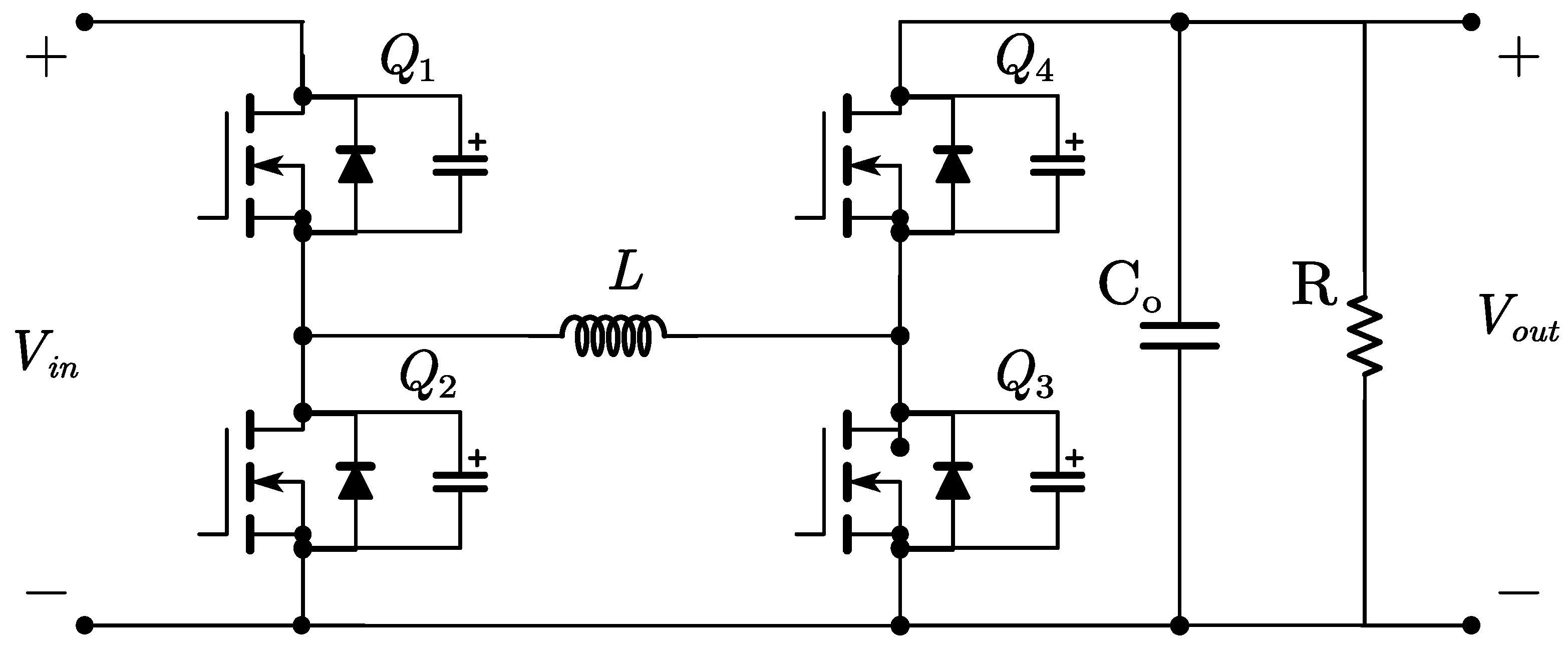
The FSBB converter circuit, shown in Figure 1, operates in either boost or buck mode, with the operating mode requiring only one branch to be modulated to achieve the target voltage. In buck—boost mode, Q1 and Q2 in Figure 1 are switched on and off simultaneously. Despite the simple structure of the FSBB circuit, few models account for both duty cycle and phase-shift angle transformations at the input/output. Literature [6,7,8] have proposed modeling approaches that ignore the duty cycle and phase-shift variations. The literature [9] considers duty cycle and phase-shift variations and implements zero-voltage switching operation, but the variables are interdependent, limiting the validity of the model. The modeling approach proposed in the literature [10] considers the effect between duty cycle and phase shift, but the mathematical model is more complex. In this paper, we consider the phase shift between the two branches while simplifying the mathematical model to develop a nonlinear average model for the FSBB converter.
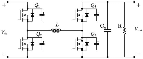
Figure 1.
The FSBB converter circuit.
One of the major challenges of FSBB converter systems is the complexity of the control methodology and its impact on overall system performance. The Proportional-Integral-Derivative (PID) control regulator is widely used in industrial control systems due to its strong adaptability and robustness. However, as industrial production systems become more complex, exhibiting characteristics such as hysteresis, time-variance, and nonlinearity, traditional PID controllers struggle to accurately regulate these systems. In recent years, neural network-based controllers have demonstrated their effectiveness in DC—DC converter systems. These controllers can function both offline and online, with dynamic responses optimized by adjusting the neural network weights, thereby improving overall system performance. Researchers have proposed several intelligent PID controllers, including expert PID, fuzzy PID, neural network PID, and backpropagation (BP) neural network PID. Each method has its own advantages and limitations. For instance, expert PID control relies on accumulated knowledge from its knowledge base, but if the experience value is inaccurate, the expected control effect will not be achieved [11]. Fuzzy control has a high tolerance for system faults but lacks precision in control accuracy [12]. Neural network-based PID controllers, on the other hand, offer online estimation and self-learning capabilities, and can approximate any nonlinear function. Moreover, their regulation process does not depend on the system model, making them well-suited for controlling FSBB converters [13,14]. The high robustness and fault tolerance of neural network algorithms make them ideal for complex nonlinear control systems [15,16]. Additionally, neural networks have a wide range of potential applications and significant development prospects.
In this paper, modeling and simulation are conducted using MATLAB 2020a to verify the effectiveness, speed, stability, and accuracy of the proposed control strategy and modeling method. Moreover, the zero-voltage switching (ZVS) operation of all the switching tubes is achieved. The rest of this paper is organized as follows. In Section 2, a review of the converter modes of operation is presented. In Section 3, the proposed modeling approach and the derivation process are presented, and the modeling approach is validated using MATLAB 2020a. In Section 4, a neuro-adaptive controller is proposed. Section 5 reports the experimental validation of the simulation. In Section 6, the content of this paper is summarized.
2. FSBB Converter Operating Mode Review
2.1. Review of FSBB Converter Operation Modes
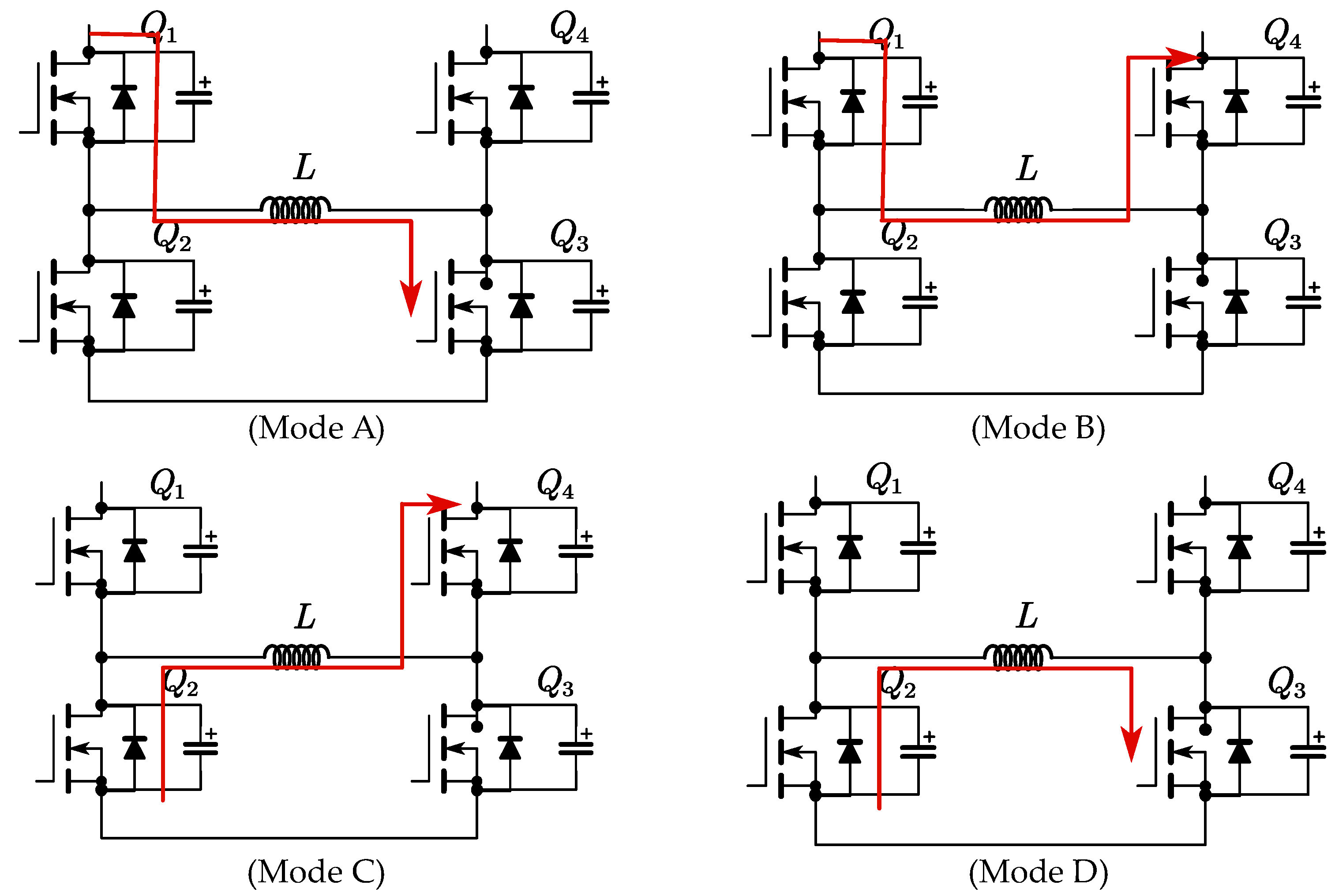
The FSBB converter is designed to achieve power conversion through the periodic switching of four switches. The output voltage is controlled by varying the switching states and cycles. The FSBB controller operates in four distinct switching modes, as illustrated in Figure 2. Operating Mode A: switching tubes Q1 and Q3 conduct, forming a Vin-Q1-L-Q3-Vin path, with an inductor voltage stress of Vin. Operating mode B: switching tubes Q1 and Q4 conduct, forming a Vin-Q1-L-Q4-Vout path, with an inductor voltage stress of Vin-Vout. Operating mode C: switching tubes Q2 and Q4 conduct, forming a Q2-L-Q4-Vout path, with an inductor voltage stress of Vout. Operating mode D: switching tubes Q2 and Q3 conduct, forming a Q2-L-Q3 path, with an inductor voltage stress of 0.

Figure 2.
Four Modes of Operation for the FSBB Converter. (Mode A), (Mode B), (Mode C) and (Mode D) are schematic diagrams of the operation of the four modes respectively.
In buck mode, Q3 is always active, while Q4 remains deactivated. Q1 and Q2 are alternately switched on, and the operating states combine Modes B and C, as illustrated in Figure 2. In boost mode, Q1 is always on, and Q2 is always off. Q3 and Q4 are alternately switched, and the operating states combine Modes A and B. In buck-boost mode, all four switching tubes are controlled to operate simultaneously. The operating states combine Modes A and C.
2.2. ZVS Conditions
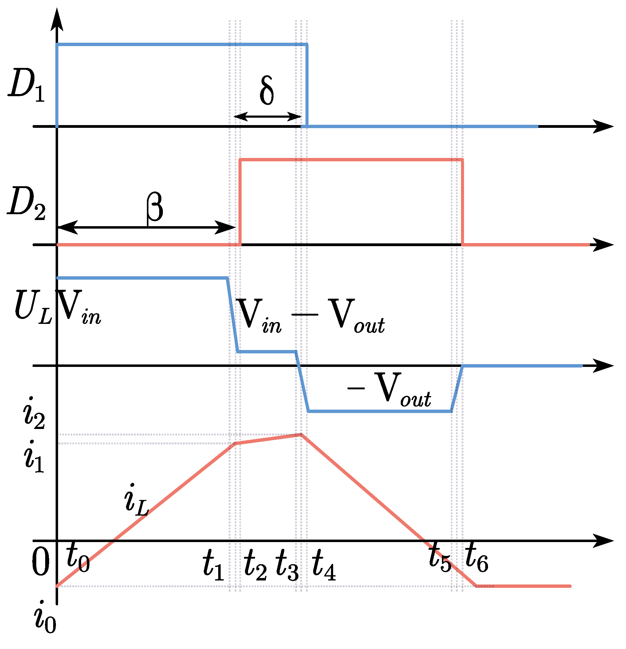
The principal waveform of the FSBB converter is illustrated in Figure 3. Here, D1 represents the input duty cycle, while D2 denotes the output duty cycle. The phase shift β denotes the time interval between the two duty cycles, while δ refers to the time when the two duty cycles coexist, which can be expressed as:

Figure 3.
The main waveforms of the FSBB converter.
At the point at which D1 overtakes D2 (β > 0),
When D2 overtakes D1 (β < 0),
The literature [17,18,19] discusses the quadrilateral inductor current mode ZVS modulation and proposes a control method based on this discussion. The ZVS condition can be rewritten as follows:
where Cr is the capacitance in parallel with the switch, and is the switch’s dead time. After simplifying the ZVS condition, it can be expressed as:
where satisfies Equation (5)
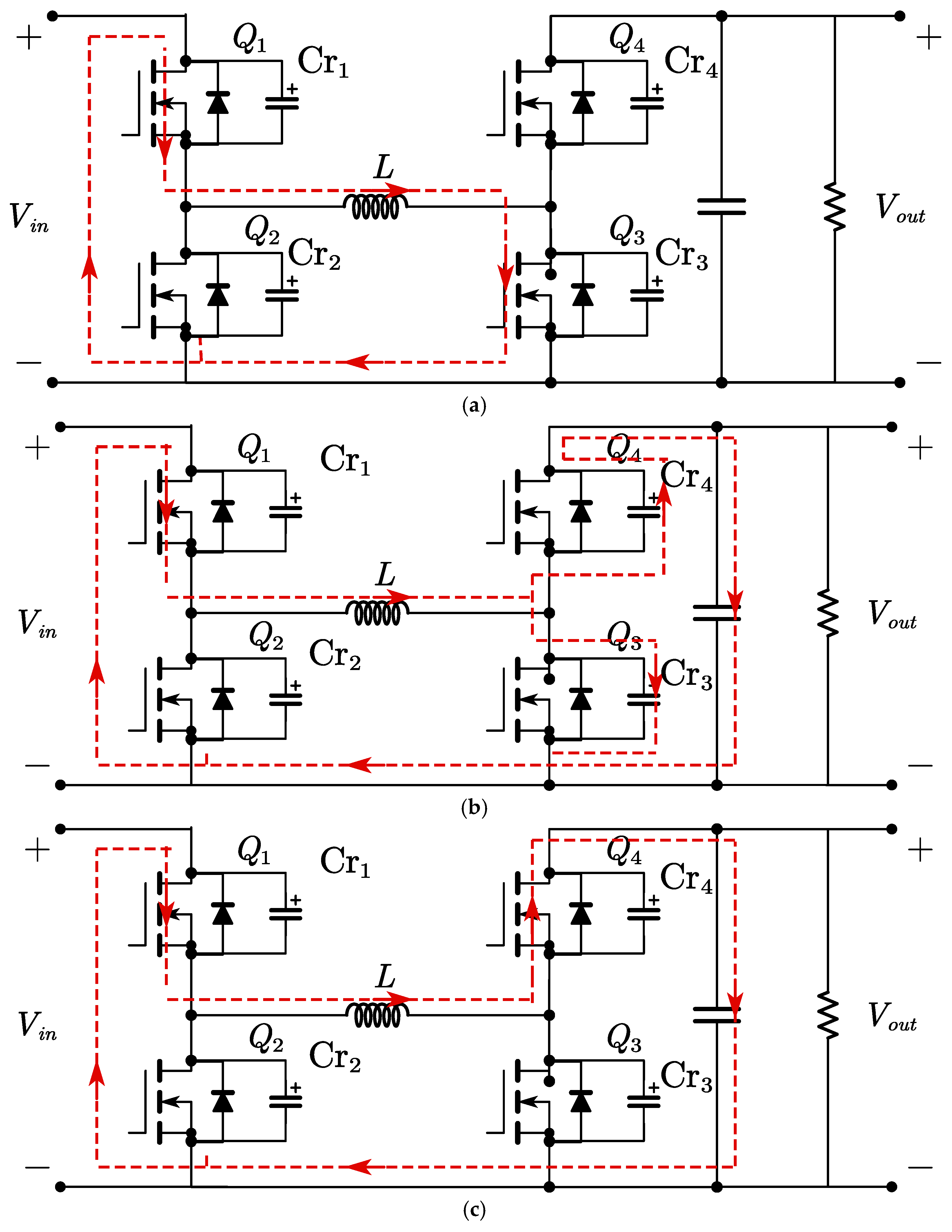
The ZVS process is as follows. From t0 to t1, the circuit operates in A mode, with the current rising to Vin/L and the output current (Io) reaching zero. Between t1 and t2, the forward current of the inductor is employed to discharge the parasitic capacitance of the Q4 switching. This causes Vcr4 to decrease to 0. At this point, the anti-parallel diode of Q4 begins to conduct, thereby clamping the voltage of Q4 at zero. This allows Q4 to be turned on, thereby achieving the zero-voltage turn-on of the switching tube Q4. Activation of tube Q3 results in a voltage of 0 on the parasitic capacitor at the t2 instant. Subsequent deactivation of Q3 leads to a transfer of input current from Q3 to the parasitic capacitor, which begins to charge. The voltage rises linearly from 0 due to the gradual increase in parasitic capacitance, causing Q3 to enter a zero-voltage shutdown state. This process is illustrated in Figure 4.
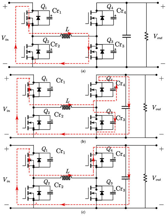
Figure 4.
Soft-switching implementation process diagram. (a–c) Composition of a duty cycle.
3. Mathematical Modeling of FSBB Converter
3.1. Modeling Analysis Based on Energy Transformation
In accordance with the law of conservation of energy, the discrepancy between the input and output ports of the FSBB controller represents the energy consumed by the inductor. This implies that the energy entering the controller during a cycle () is equal to the integral of the product of the input voltage and input current over the cycle duration. This is expressed as:
where Ts is the duration of one cycle. The energy flux exiting the output port is given by the following expression:
The energy stored in the inductor, represented by the variable , is the difference between the energy at the input and output ports. This can be expressed as:
The energy at the input can be decomposed into two distinct components: the first is related to the initial current () and the other is associated with the inductor current when the switch is on. Similarly, the energy at the output can be decomposed into a component related to the current at the final moment and the inductor current when the switch is on. The relationship between and can be expressed as:
where fs is the switching frequency, D1 is the duty cycle of input, and D2 is the duty cycle of output. The inductor current () undergoes periodic variation during the converter operation. Combining Equations (2) and (3), the energy difference () can be expressed as a function of the input and output voltages ( and ), the duty cycles ( and ), and the current values ( and ):
The mean voltage ()and mean current () of the inductor over one cycle can be derived from Equation (12) and expressed as:
3.2. Deriving the Transfer Function
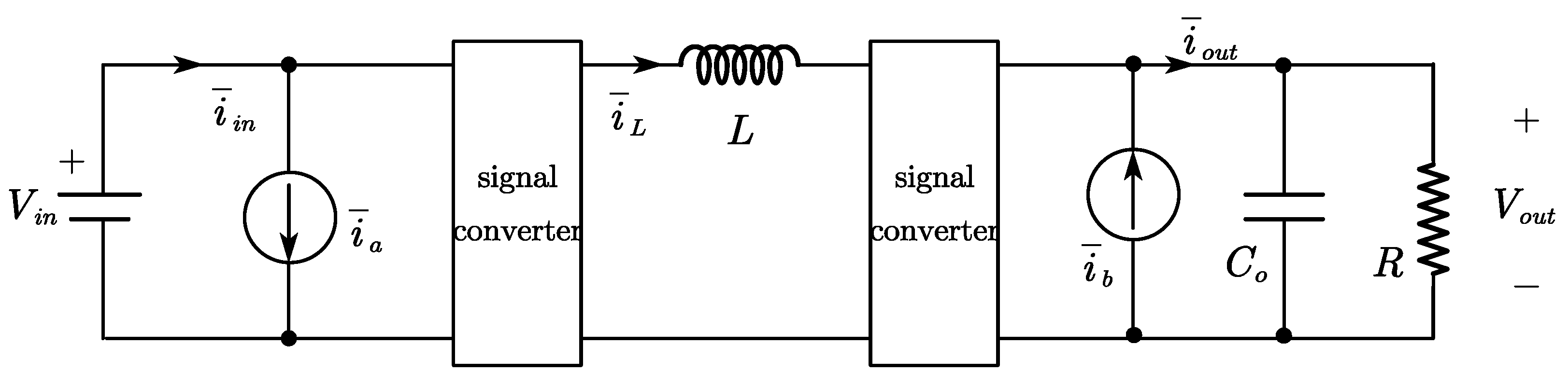
The equivalent nonlinear average model of the converter is illustrated in Figure 5. The input and output currents can be expressed as the inductor current , multiplied by and respectively, plus the additional currents and :
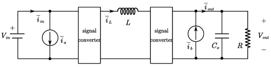
Figure 5.
Nonlinear average model of the FSBB.
The average input and output currents can be obtained by calculating the mean of the input and output currents during the switching cycle, based on the energy exchange at the ports:
The current values , and , as defined in Equations (12) and (14), can be combined to yield the following expressions:
A small-signal model can be obtained by linearizing the signal through decomposition into two parts: the steady-state component and the small signal (e.g., ). This approach retains only the first-order terms, resulting in the model shown in Figure 6. The functions represented by x and y in the figure are given by:
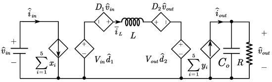
Figure 6.
Linear small-signal model of the FSBB.
3.3. Signal Model Validation
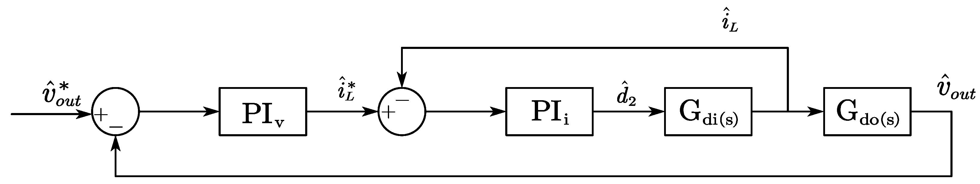
The control system described in this paper comprises an outer voltage control loop and an inner current control loop. The control block diagram is presented in Figure 7. The transfer functions of the system are given by and .

Figure 7.
Considered FSBB control structure.
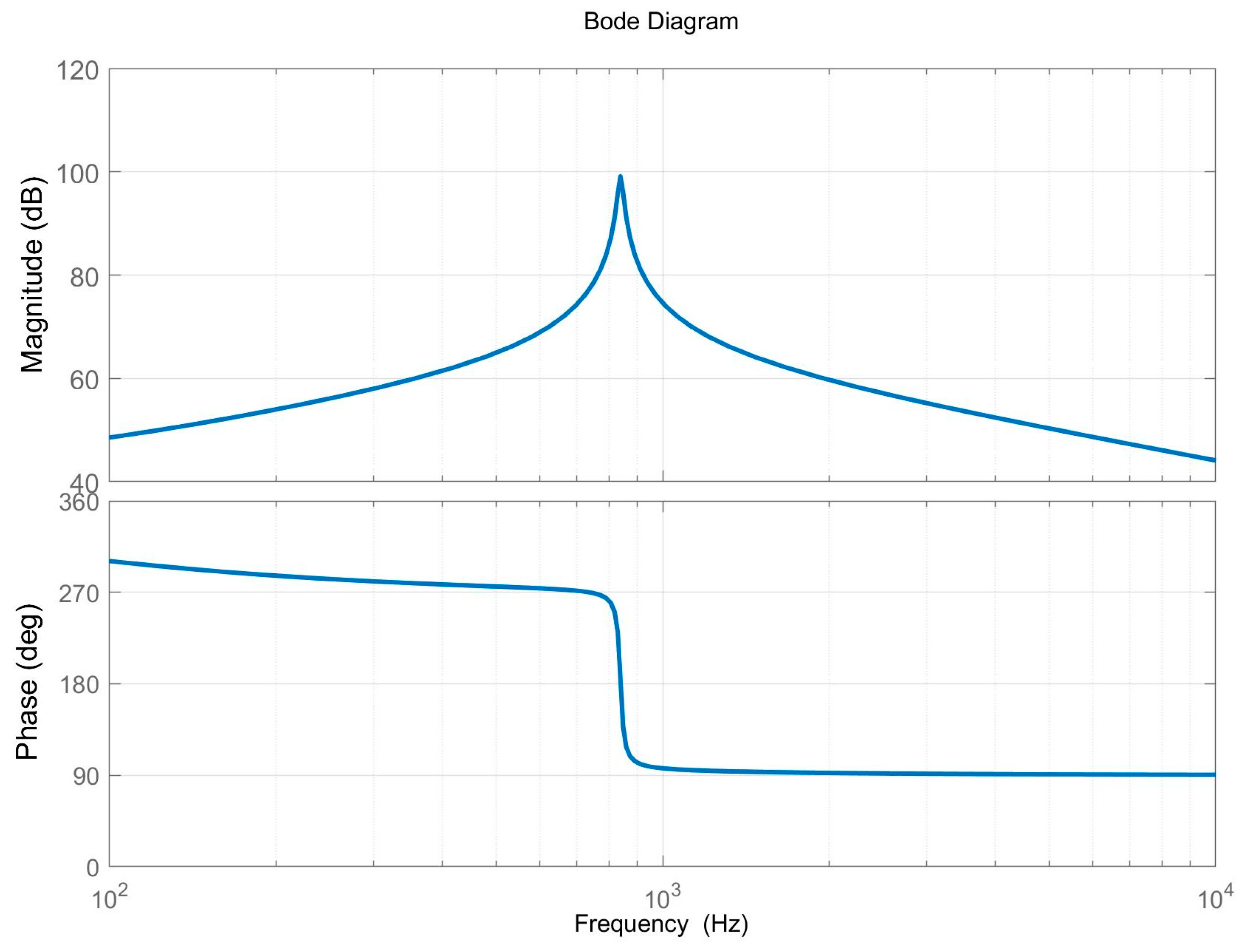
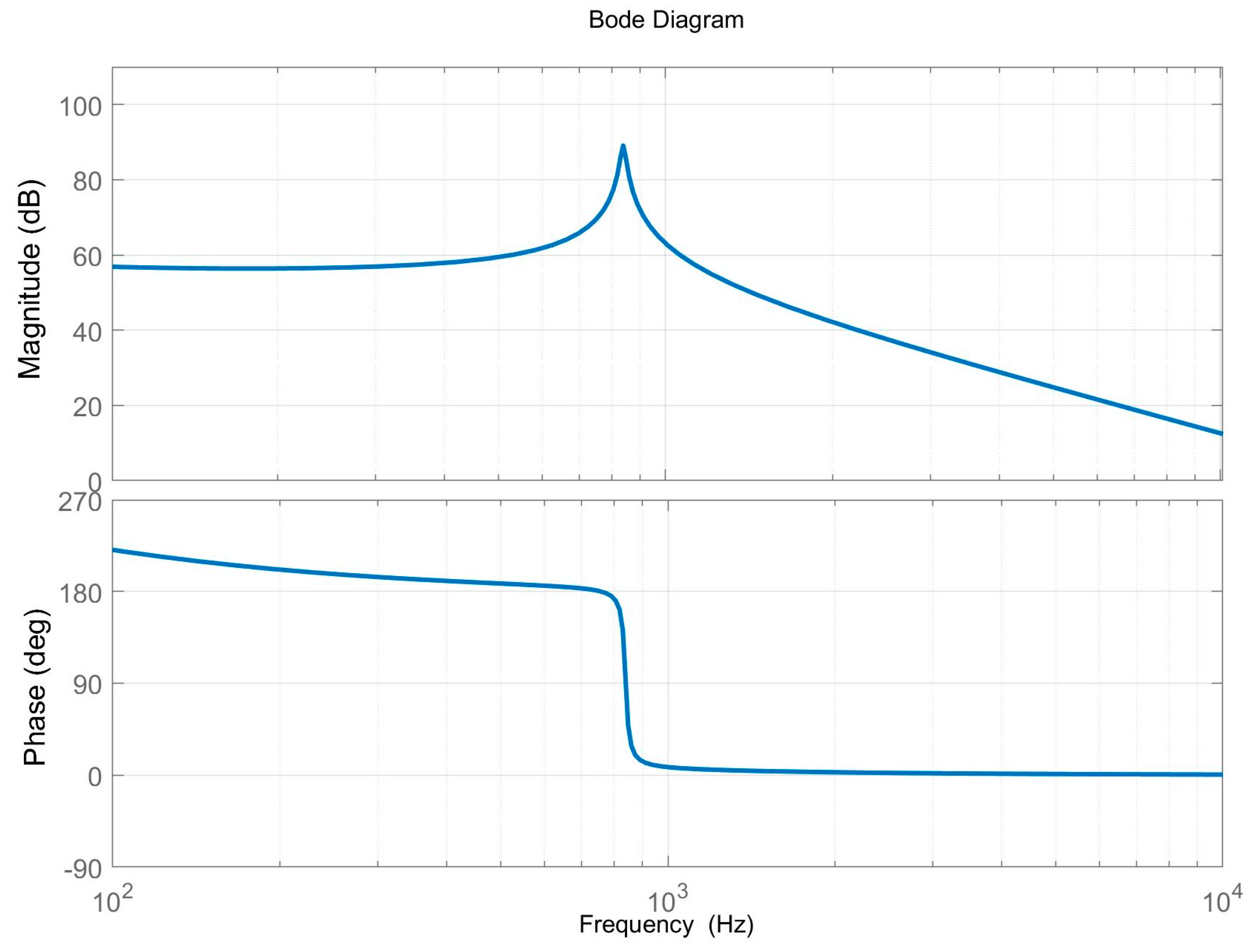
Figure 8 and Figure 9 are Bode diagrams for the transfer functions of Equations (23) and (24), respectively. As can be seen from the figures, the model correctly predicts the response over the entire frequency range under consideration. The response curve in the frequency domain shown in the figure is consistent with the theory and previous studies, which can prove the accuracy of the modeling method used.
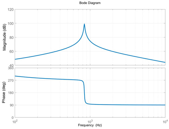
Figure 8.
Bode diagrams for the transfer functions of Equation (23).
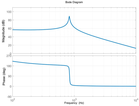
Figure 9.
Bode diagrams for the transfer functions of Equation (24).
4. Adaptive Neural Network Controller
4.1. Control Structure Design
The traditional incremental digital PID control algorithm is based on the following formula:
where kP means proportional coefficient, kI means integral coefficient, and kD means differential coefficient.
Traditional PID control tends to exhibit a degree of hysteresis, where the system output has a lagging effect on the results [20]. Additionally, in practical engineering control, many PID systems operate over extended periods, during which the system’s physical properties may change due to factors such as component replacement or corrosion. As a result, the original factory-set PID parameters may no longer be optimal for the system. Implementing an adaptive PID algorithm enables real-time adjustment of PID parameters, ensuring optimal system performance.
Compared to traditional PID control, the neural network-based PID (NN-PID) controller offers significant improvements in efficiency and adaptability. Traditional PID controllers rely on fixed parameters, which often become suboptimal over time due to changes in the system conditions, such as component aging or environmental variations. In contrast, NN-PID controllers can adaptively adjust PID parameters in real time, ensuring optimal performance across different operating scenarios. NN-PID controllers also provide faster response times and reduced overshoot. While traditional PID systems might exhibit slower convergence and significant overshoot, especially in complex or nonlinear systems, NN-PID controllers can predict system behavior and adjust control actions proactively. This results in quicker stabilization and more stable output with minimal overshoot, improving overall system reliability.
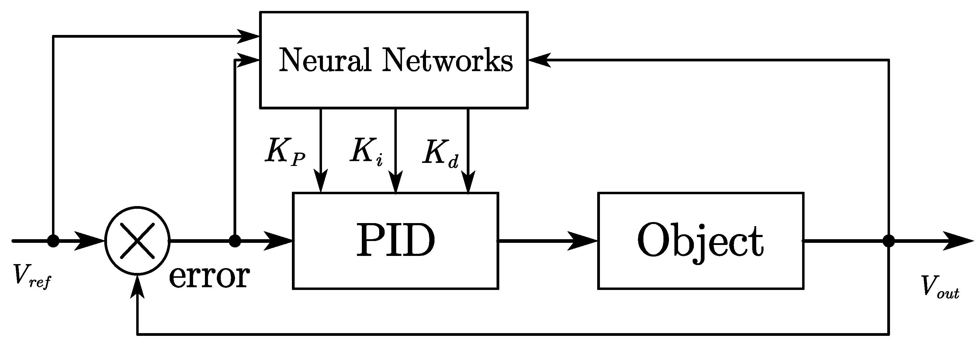
This paper proposes a method for achieving self-adaptive control of the PID parameters using a neural network system, with the objective of enhancing controller performance. The structure of this system is illustrated in Figure 10.
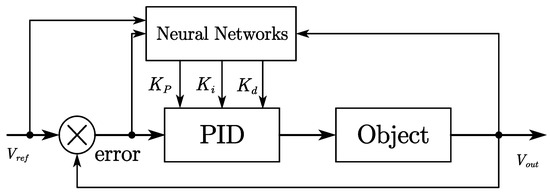
Figure 10.
Improved neural network controller structure.
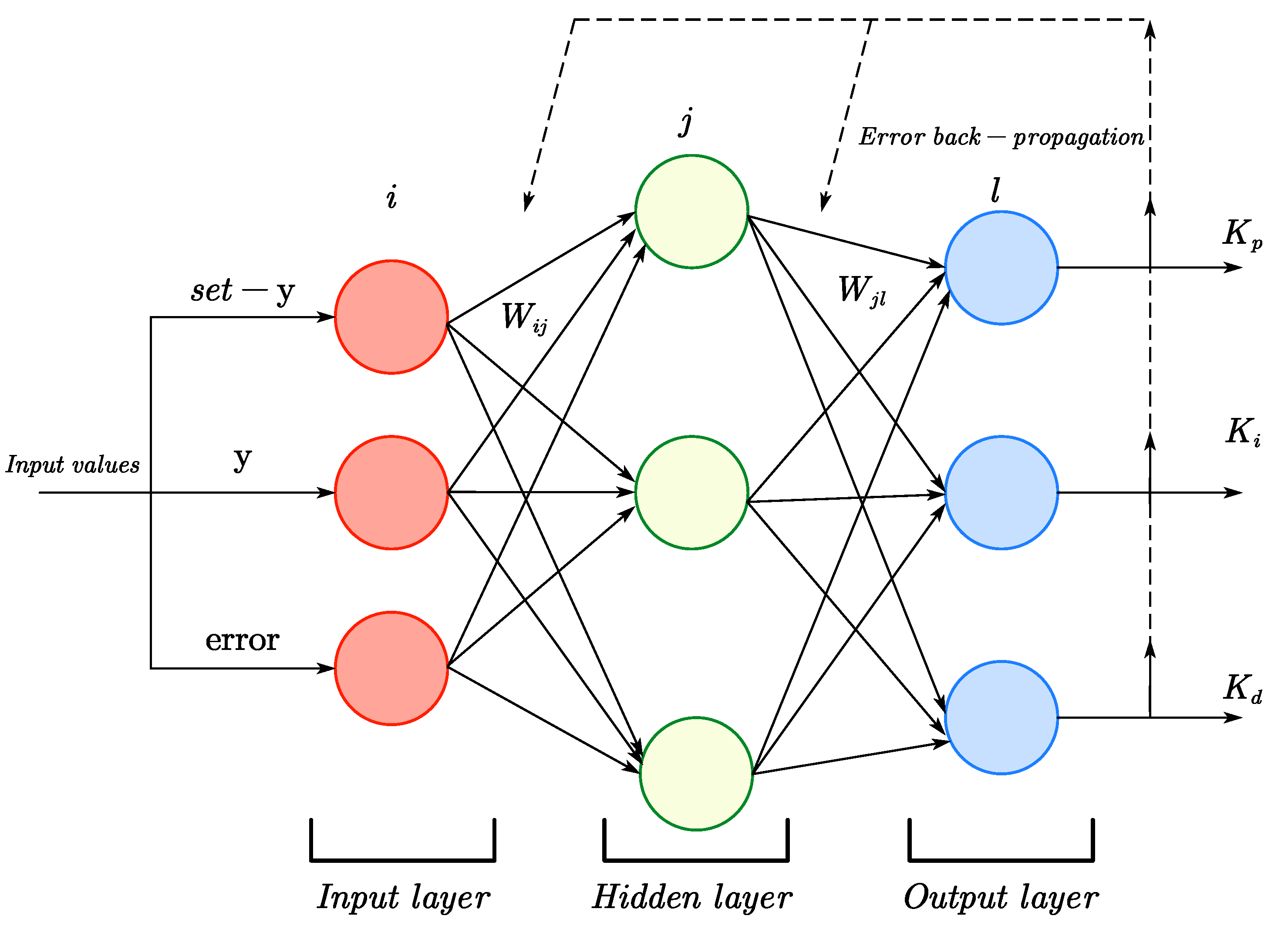
4.2. BP Neural Network Control Algorithm
The gradient steepest descent method, a fundamental principle of BP neural networks, is used to minimize the mean-square deviation between the actual output of the controller and the desired output. This is achieved through a self-learning process that adjusts the weights of the network to move towards the desired value.
Figure 11 illustrates the training structure of the BP neural network, which consists of an input layer, a hidden layer, and an output layer. In this paper, the number of neurons in the input, hidden, and output layers is three. The hidden layer is responsible for forward propagation and calculating the output, which is then adjusted, and the error is propagated back to the input layer. Continuous adjustment of the BP neural network weights reduces the error over time, improving the accuracy of the training samples and achieving the desired output.

Figure 11.
Training structure of BP neural network.
Since the output layer nodes represent kP, kI and kD, which must be non-negative, a non-negative hyperbolic tangent function is chosen as the activation function for this layer:
Its derivative is:
where the input layer inputs are:
The implicit layer inputs are:
The implicit layer output is:
The output layer inputs are:
The output layer output is:
Selection of the performance indicator function E(k) is made according to the specifications set forth in Equation (25).
In accordance with the gradient descent rule, when the learning rate is set to η, the adjustment of the connection weights of the output layer at the current moment (k time) is as follows:
where
Once the connection weights of the output layer have been simplified and approximated, the resulting change in these weights after the learning process is as follows:
where
The connection weights of the output layer at time k are updated to:
The degree of alteration in the implicit layer connection weights subsequent to the learning process is as follows:
In accordance with the solution step for the output layer, the degree of alteration in the connection weights of the implicit layer subsequent to the learning process can be determined as follows:
where
4.3. Adaptive Optimization of the Output
The absolute value of the discrepancy between the predicted value of samples of the PID control and the anticipated value as the individual fitness function is expressed as follows:
where i = 1, 2, 3, …, n; n is the number of training samples.
- is the expected value.
- is the predicted value.
A lower fitness value indicates a smaller sum of absolute errors, which in turn signifies enhanced network performance. Accordingly, the enhanced BP neural network model presented in this paper employs the sum of the absolute values of the discrepancies between the predicted and anticipated values of the PID control as the global fitness function, which is expressed as follows:
In order to enhance the control performance of the controller and make it meet the demand of the actual converter, the adaptive control rate is added to the output layer of the neural network. The exponential function of the limiting is selected as the generating function of the adaptive control signal, and the absolute value of the voltage error of equal scale reduction is selected as the input of x. The formula is shown as Equation (44), where KA, KB, and KC are the compensation parameters of the proportional integral and differential, respectively. According to practical engineering experience, the compensation parameters of proportional integral and differential need to be designed separately, and their values follow 1:2.5:0.0000025. The device may be designated the EA-BP PID controller.
4.4. Analysis of Control System
In this section, a simulation was carried out using the energy model and the double closed-loop control system proposed above. The data in Table 1 were used in Equations (23) and (24) to obtain the transfer functions. The conventional PID controller and the EA-BP PID controller proposed in this paper were then compared.

Table 1.
List of parameters used in the simulation.
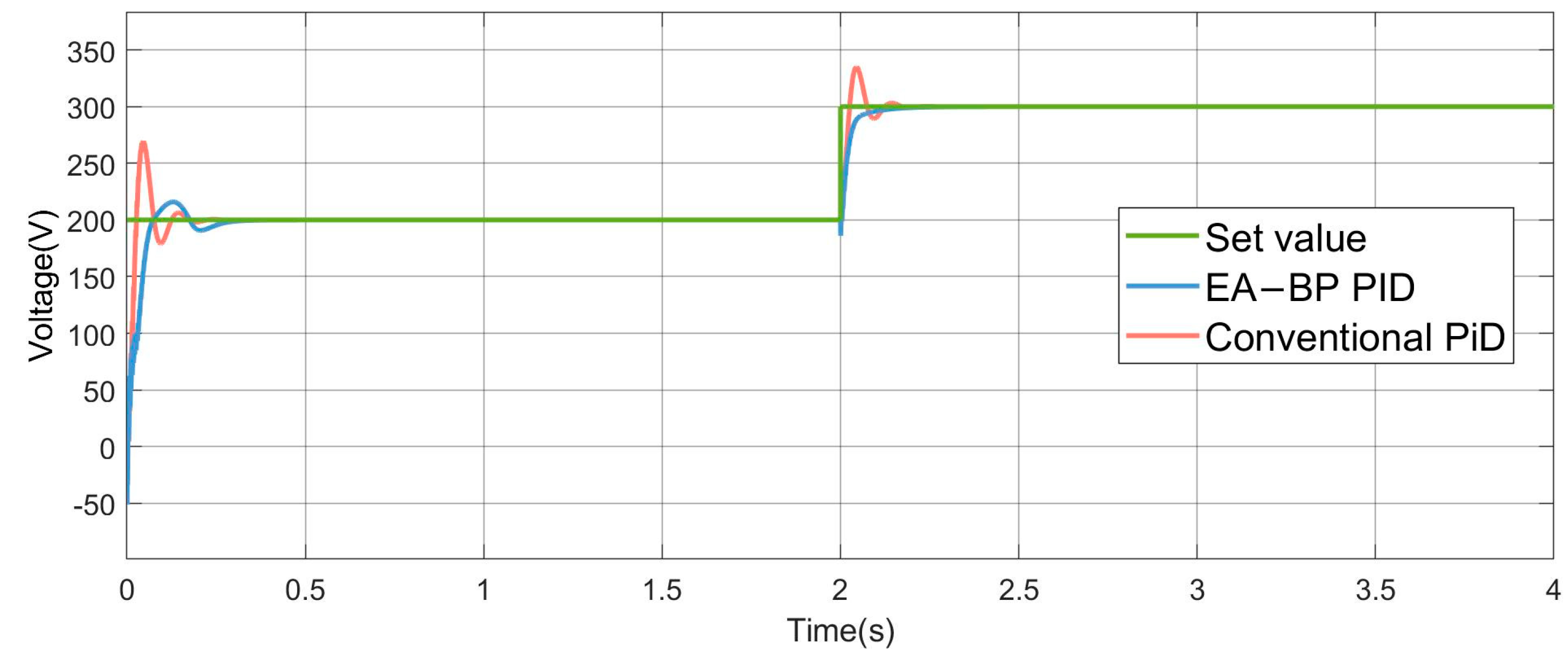
Figure 12 shows the output performance of the traditional PID controller and the adaptive PID controller. Comparing the results, the traditional PID controller exhibited a voltage overshoot of 33% and 11.3% before reaching a steady state, while the adaptive controller showed no significant overshoot and responded more quickly.
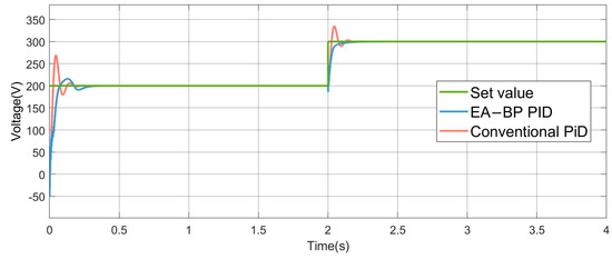
Figure 12.
The resulting graph from the output.
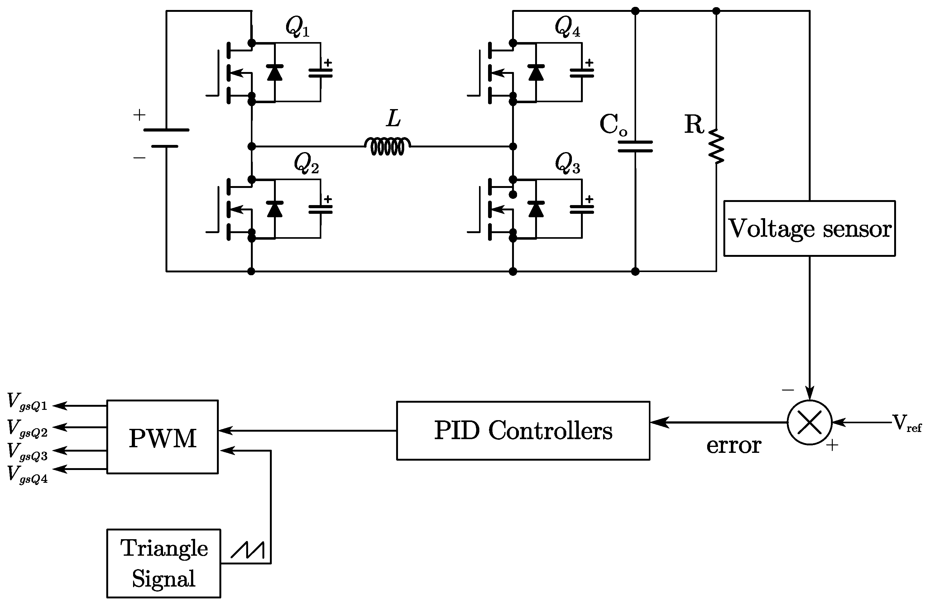
5. Analysis of Simulation Results
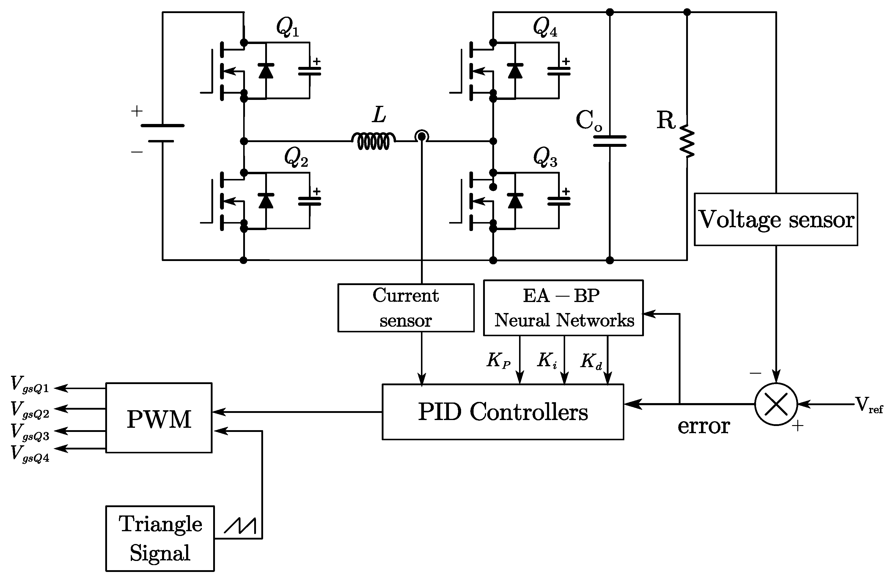
The block diagram of the proposed closed-loop control system is shown in Figure 13, while the classical PID controller block diagram is depicted in Figure 14. The output voltage is sampled by a voltage sensor at the output side, and the error signal is transmitted to the neural network-based PID controller, which has been designed in accordance with the specifications outlined in this paper, to generate the control waveform. The control signal for the switch is then transmitted to the FSBB controller using the pulse width modulation (PWM) method, thereby completing the closed-loop control.

Figure 13.
Block diagram representing a proposed controller.

Figure 14.
Classical PID controller block diagram.
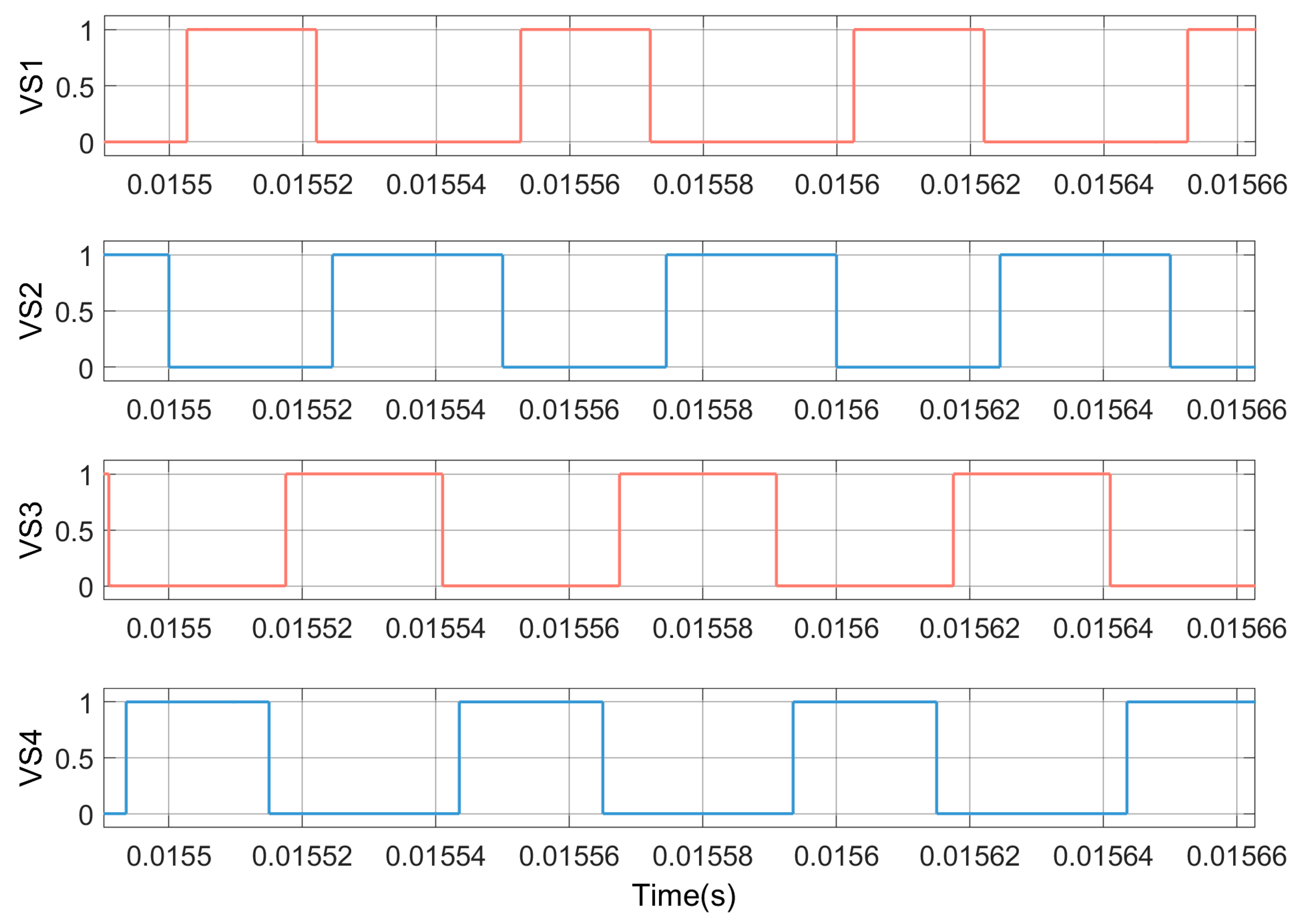
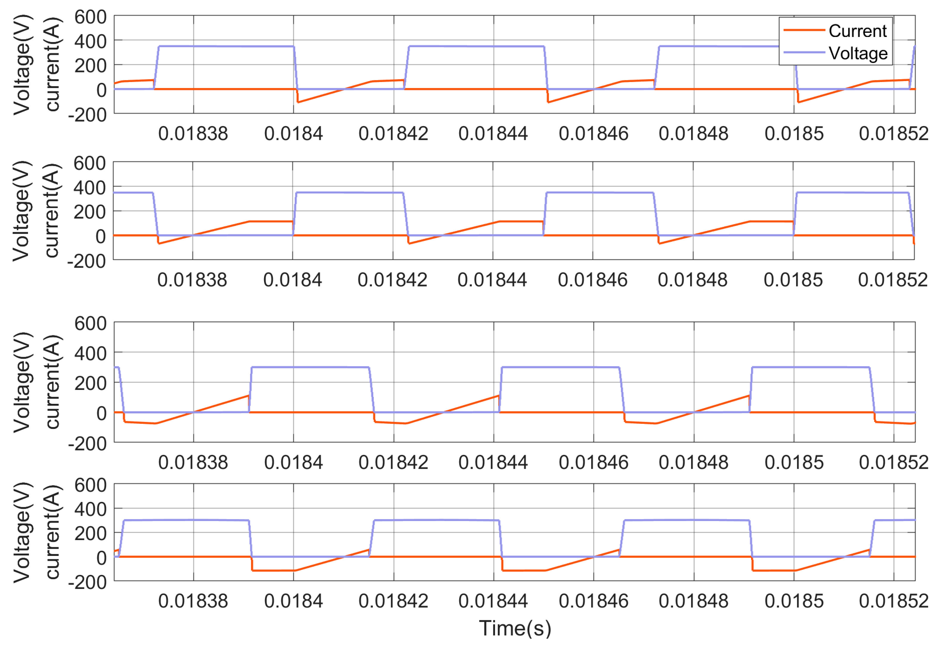
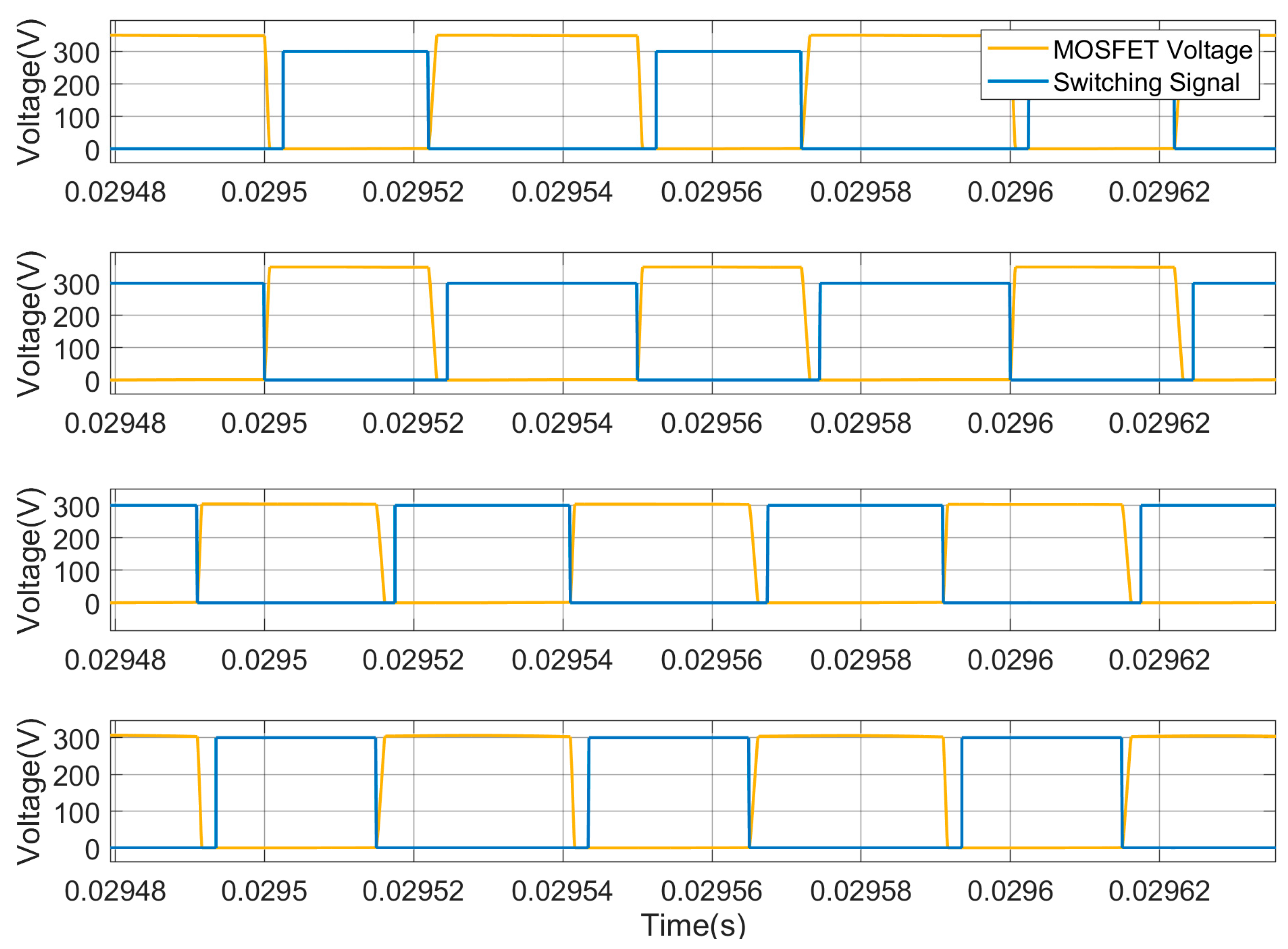
In this section, the FSBB converter is modeled and validated using the parameters listed in Table 1. Figure 15 illustrates the switching states of Q1, Q2, Q3, and Q4, respectively. The driving signals for these switching transistors are VS1, VS2, VS3, and VS4, respectively. The voltage and current curves for the switching transistors are shown in Figure 16, where it can be observed that there is no overlap between the two curves. Figure 17 illustrates the switching transistor drive signals and voltage signals, demonstrating that the transistors undergo a transition at a voltage of 0, thus achieving zero-voltage switching (ZVS).
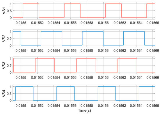
Figure 15.
The switching states.
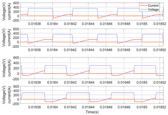
Figure 16.
The voltage and current curves for the switching tubes.
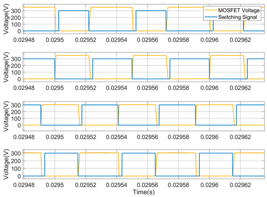
Figure 17.
The switching tube drive signals and voltage signals.
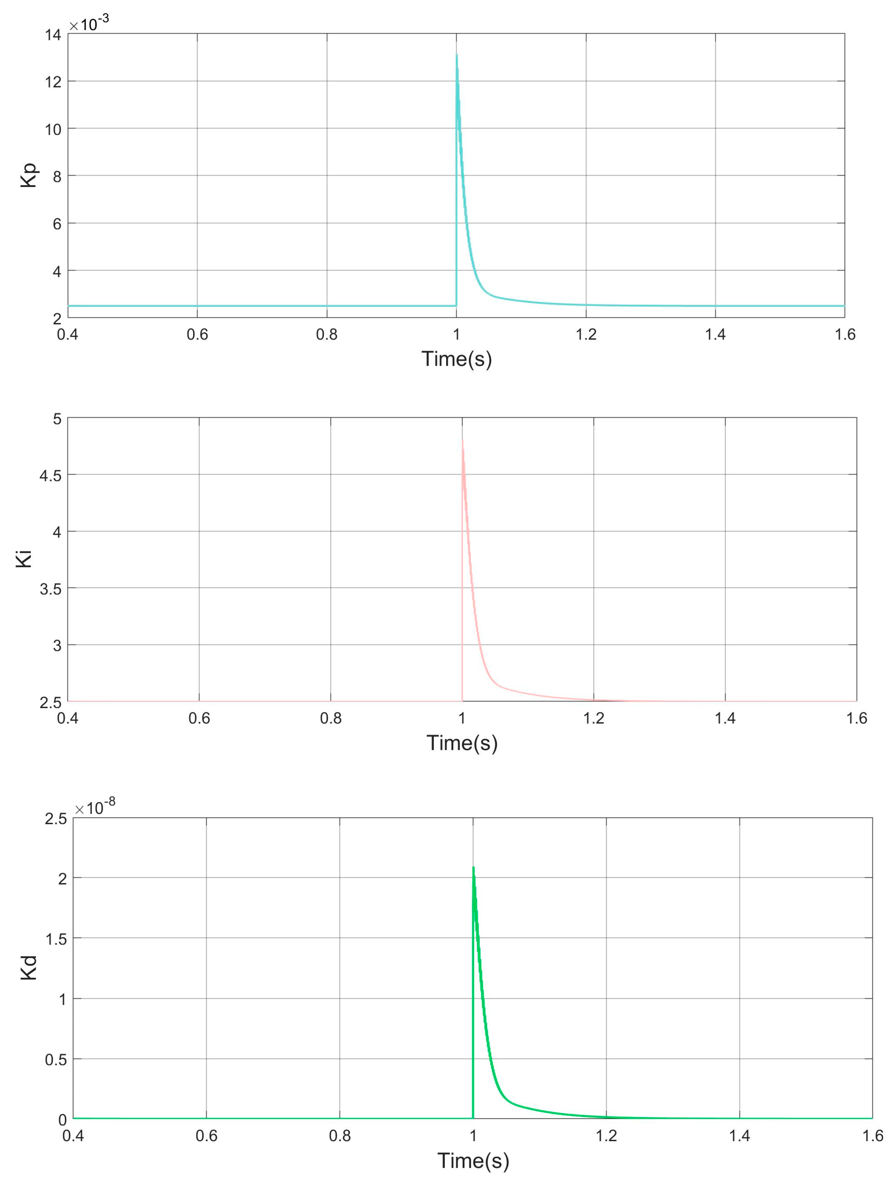
In order to verify the adaptivity of the controller, an experiment was designed. The set voltage was changed at 1 s to observe the changes in the controller parameter outputs, and the experimental results are shown in Figure 18. From the experimental results, it can be concluded that all three parameters automatically return to the smooth working state within 0.2 s.

Figure 18.
Controller parameter diagram.
Figure 19 presents the output voltage and current plots of the PID controller and the neural network-based PID controller proposed in this paper under identical conditions. The converter is considered to be in steady state when the voltage variation is less than 1% of the output voltage. Before reaching a steady state, the conventional PID converter exhibited a 10% voltage overshoot. The voltage overshoot of the conventional PID controller is significantly higher than that of the EA-BP PID controller proposed in this study. Moreover, the traditional PID controller took 0.3 s to reach a steady state, whereas the EA-BP PID controller reached a steady state in just 0.02 s, indicating a much faster response time. Additionally, after prolonged operation, the output waveform of the traditional PID controller exhibited considerable disturbance, while the new PID controller demonstrated superior stability and maintained a consistent operating state.
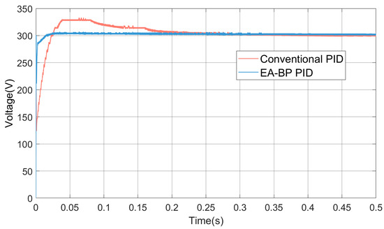
Figure 19.
Output voltage comparison diagram under rated working conditions.
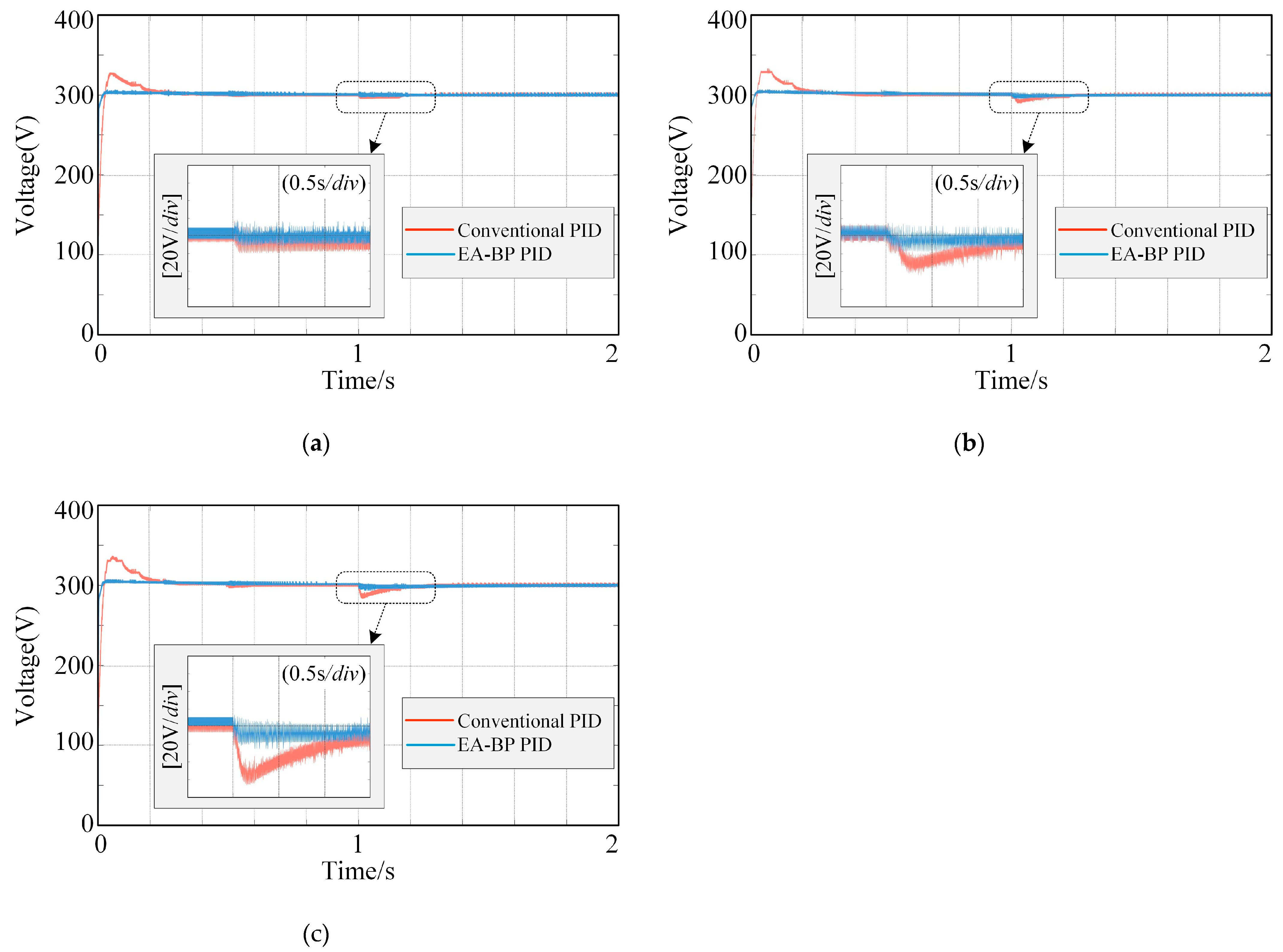
In this study, the FSBB converter is rated at 3 kW, and different resistor values corresponding to various power levels were set according to Table 2 to verify the wide load range of this controller. The results are shown in Figure 20. To further explore the regulation capabilities of the converter, the load was altered at 1 s. To evaluate the dynamic performance of the rectifier converter (specifically its load range), the converter’s load was increased from light load conditions to full load at 1 s. The light load power levels were set at 20%, 50%, and 80%, respectively. It was observed that the EA-BP PID controller quickly reached a steady state after the load was altered.
Table 2.
List of parameters.

Figure 20.
Load voltage at different power variations. (a) 20% power variation. (b) 50% power variation. (c) 80% power variation.
6. Discussion
This paper proposes a novel adaptive PID control scheme based on an improved BP neural network for a four-switch buck—boost (FSBB) converter, with the goal of achieving zero-voltage switching (ZVS) for all four switches. In the construction of the nonlinear average model and the corresponding small-signal model, a novel modeling approach based on energy variation was employed to avoid the need for redundant processing calculations or additional hardware modifications at a later stage.
The enhanced BP neural network improves the PID control performance of the FSBB converter by enabling parameter self-adaptation, thereby addressing the limitations of traditional PID controllers. This approach offers a valuable reference for the development and design of high-efficiency intelligent FSBB DC—DC converters. To further improve the PID control performance of the FSBB DC converter, future studies should investigate more advanced optimization algorithms.
Author Contributions
Conceptualization, L.R. and Y.Z.; methodology, L.R.; software, Y.Z.; validation, L.R., D.W. and Y.Z.; formal analysis, L.R.; investigation, Y.Z.; resources, D.W.; data curation, Y.Z.; writing—original draft preparation, L.R.; writing—review and editing, L.R.; visualization, Y.Z.; project administration, D.W.; funding acquisition, D.W. All authors have read and agreed to the published version of the manuscript.
Funding
This study received no external funding.
Data Availability Statement
The data are contained within the article.
Conflicts of Interest
The authors declare no conflicts of interest.
References
- Wang, Y.-F.; Xue, L.-K.; Wang, C.-S.; Wang, P.; Li, W. Interleaved High-Conversion-Ratio Bidirectional DC–DC Converter for Distributed Energy-Storage Systems—Circuit Generation, Analysis, and Design. IEEE Trans. Power Electron. 2016, 31, 5547–5561. [Google Scholar] [CrossRef]
- Zhu, J.-Y.; Lehman, B. Control Loop Design for Two-Stage DC-DC Converters with Low Voltage/High Current Output. IEEE Trans. Power Electron. 2005, 20, 44–55. [Google Scholar] [CrossRef]
- Ruan, X.; Li, B. Zero-Voltage and Zero-Current-Switching PWM Hybrid Full-Bridge Three-Level Converter. IEEE Trans. Ind. Electron. 2005, 52, 213–220. [Google Scholar] [CrossRef]
- Ruan, X.; Chen, Z.; Chen, W. Zero-Voltage-Switching PWM Hybrid Full-Bridge Three-Level Converter. IEEE Trans. Power Electron. 2005, 20, 395–404. [Google Scholar] [CrossRef]
- Pesce, C.; Blasco, R.; Riedemann, J.; Andrade, I.; Pena, R. A DC-DC Converter Based On Modified Flyback Converter Topology. IEEE Latin Am. Trans. 2016, 14, 3949–3956. [Google Scholar] [CrossRef]
- Kwon, H.-J.; Kim, K.-Y.; Kim, J.-H. A Novel Control Scheme of Four Switch Buck-Boost Converter for Super Capacitor Pre-Charger. IEEE Access 2024, 12, 47210–47218. [Google Scholar] [CrossRef]
- Chen, Z.; Tang, X.; Zheng, Z.; Wu, Y.; Luo, Z. An Adaptive Dual-controller On-line Efficiency Optimization Method of Four-switch Buck-boost Converter for Wide Range Application. Int. J. Circuit Theory Appl. 2024, 52, 2686–2703. [Google Scholar] [CrossRef]
- González-Castaño, C.; Restrepo, C.; Flores-Bahamonde, F.; Rodriguez, J. A Composite DC–DC Converter Based on the Versatile Buck–Boost Topology for Electric Vehicle Applications. Sensors 2022, 22, 5409. [Google Scholar] [CrossRef] [PubMed]
- Bai, Y.; Cao, Y.; Mitrovic, V.; Fan, B.; Burgos, R.; Boroyevich, D. A Simplified Quadrangle Current Modulation for Four-Switched Buck-Boost Converter (FSBB) with a Novel Small Signal Model. In Proceedings of the 2023 IEEE Applied Power Electronics Conference and Exposition (APEC), Orlando, FL, USA, 19 March 2023; IEEE: New York, NY, USA, 2023; pp. 736–743. [Google Scholar]
- Gallo, E.; Biadene, D.; Cvejić, F.; Spiazzi, G.; Caldognetto, T. An Energy-Based Model of Four-Switch Buck–Boost Converters. IEEE Trans. Power Electron. 2024, 39, 4139–4148. [Google Scholar] [CrossRef]
- Xu, X.; Li, D. Torque Control of DC Torque Motor Based on Expert PID. J. Phys. Conf. Ser. 2020, 1626, 012073. [Google Scholar] [CrossRef]
- Bello, A.; Olfe, K.S.; Rodríguez, J.; Ezquerro, J.M.; Lapuerta, V. Experimental Verification and Comparison of Fuzzy and PID Controllers for Attitude Control of Nanosatellites. Adv. Space Res. 2023, 71, 3613–3630. [Google Scholar] [CrossRef]
- Zhang, M.-L.; Zhang, Y.-J.; He, X.-L.; Gao, Z.-J. Adaptive PID Control and Its Application Based on a Double-Layer BP Neural Network. Processes 2021, 9, 1475. [Google Scholar] [CrossRef]
- Zhang, H.; Yuan, X. An Improved Ppaper Swarm Algorithm to Optimize PID Neural Network for Pressure Control Strategy of Managed Pressure Drilling. Neural Comput. Appl. 2020, 32, 1581–1592. [Google Scholar] [CrossRef]
- Ma, C.; Tian, S.; Xiao, X.; Jiang, Y. Fuzzy Neural Network PID–Based Constant Deceleration Compensation Device for the Brakes of Mining Hoists. Adv. Mech. Eng. 2020, 12, 168781402093756. [Google Scholar] [CrossRef]
- Cheng, Y.-M.; Liu, C.; Wu, J.; Liu, H.-M.; Lee, I.-K.; Niu, J.; Cho, J.-P.; Koo, K.-W.; Lee, M.-W.; Woo, D.-G. A Back Propagation Neural Network with Double Learning Rate for PID Controller in Phase-Shifted Full-Bridge Soft-Switching Power Supply. J. Electr. Eng. Technol. 2020, 15, 2811–2822. [Google Scholar] [CrossRef]
- Shen, Y.; Jiang, Y.; Zhao, H.; Shillaber, L.; Jiang, C.; Long, T. Quadrilateral Current Mode Paralleling of Power MOSFETs for Zero-Voltage Switching. IEEE Trans. Power Electron. 2021, 36, 5997–6014. [Google Scholar] [CrossRef]
- Liu, F.; Xu, J.; Chen, Z.; Huang, R.; Chen, X. A Constant Frequency ZVS Modulation Scheme for Four-Switch Buck–Boost Converter With Wide Input and Output Voltage Ranges and Reduced Inductor Current. IEEE Trans. Ind. Electron. 2023, 70, 4931–4941. [Google Scholar] [CrossRef]
- Zhou, Z.; Li, H.; Wu, X. A Constant Frequency ZVS Control System for the Four-Switch Buck–Boost DC–DC Converter With Reduced Inductor Current. IEEE Trans. Power Electron. 2019, 34, 5996–6003. [Google Scholar] [CrossRef]
- Li, H.; Tong, Y.; Li, C. Modeling and Control of a Linear Piezoelectric Actuator. Actuators 2024, 13, 55. [Google Scholar] [CrossRef]


Disclaimer/Publisher’s Note: The statements, opinions and data contained in all publications are solely those of the individual author(s) and contributor(s) and not of MDPI and/or the editor(s). MDPI and/or the editor(s) disclaim responsibility for any injury to people or property resulting from any ideas, methods, instructions or products referred to in the content. |
© 2024 by the authors. Licensee MDPI, Basel, Switzerland. This article is an open access article distributed under the terms and conditions of the Creative Commons Attribution (CC BY) license (https://creativecommons.org/licenses/by/4.0/).