Abstract
The control of the injection speed in hydraulic injection molding machines is critical to product quality and production efficiency. This paper analyzes servomotor-driven constant pump hydraulic systems in injection molding machines to achieve optimal tracking control of the injection speed. We propose an efficient reinforcement learning (RL)-based approach to achieve fast tracking control of the injection speed within predefined time constraints. First, we construct a precise Markov decision process model that defines the state space, action space, and reward function. Then, we establish a tracking strategy using the Deep Deterministic Policy Gradient RL method, which allows the controller to learn optimal policies by interacting with the environment. Careful attention is also paid to the network architecture and the definition of states/actions to ensure the effectiveness of the proposed method. Extensive numerical results validate the proposed approach and demonstrate accurate and efficient tracking of the injection velocity. The controller’s ability to learn and adapt in real time provides a significant advantage over the traditional Proportion Integration Differentiation controller. The proposed method provides a practical solution to the challenge of maintaining accurate control of the injection speed in the manufacturing process.
1. Introduction
Injection molding is a process that involves injecting molten plastic or metal through the injection device of an injection molding machine (IMM) into a mold. After cooling and solidification, the process results in the formation of the final product. The basic principles encompass four stages: melting, injection, cooling, and demolding [1,2,3]. In an IMM, as illustrated in Figure 1, plastic raw material undergoes heating and melting processes, transforming into a molten state. Subsequently, through a precise injection mechanism, the molten material is injected into the mold cavity, forming the specific shape of the desired part or product. Throughout this process, controlling key parameters such as the injection speed, temperature, pressure, and cooling time is crucial to ensure that the dimensional accuracy, surface quality, and mechanical performance of the final product meet the design requirements.
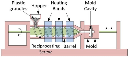
Figure 1.
Typical injection molding machine equipment.
Regulating the injection speed stands as a critical element in the injection molding process, directly influencing the quality and productivity of molded items. The primary objective of injection speed control is to uphold a consistent flow rate of molten material throughout the injection phase, thereby avoiding the occurrence of defects, such as flow marks, shrinkage, and stress. During high-speed filling, molten material experiences substantial frictional heating as it flows into the cavity via the nozzle and runner system, causing a rise in its temperature. However, an insufficient injection speed prolongs the filling time. Conversely, filling the mold cavity at a high injection speed may lead to unsatisfactory welds at the rear of the insert, consequently diminishing the strength of the product. Therefore, achieving optimal tracking control of the IMM speed is a crucial means of improving production efficiency and reducing production costs in the injection molding process. Controlling the injection speed presents a challenge due to the dynamic nature of the molten material’s physical properties, including the viscosity and specific volume, as well as quality parameters, like the temperature and pressure. These properties fluctuate over time, location, and process conditions, contributing to the nonlinearity and uncertainty inherent in molten material flow.
In the developmental trajectory of the IMM control field, scholars both domestically and internationally have conducted extensive research on speed optimization and control methods for various injection molding systems over the past few decades [4,5,6,7,8,9,10,11,12,13,14,15,16,17,18,19,20]. Currently, in the practical field of the injection molding industry, the widely applied and mature methods are still predominantly focused on traditional control methods. For example, in [21], Tan et al. proposed a learning-enhanced PI control method for the periodic control of the ram speed in IMMs. In [12], Yang et al. introduced an enhanced PID method to improve injection speed control. Yang et al. introduced an improved PID method utilizing unsaturated integration and differential elimination for enhanced injection speed control. In [22], Tian et al. employed a dual-controller scheme for injection speed control, allowing for setpoint tracking and load suppression, demonstrating excellent system robustness. Special techniques such as profile transformation and shifting were also introduced to improve speed response. In [7], Huang et al. proposed neural network-based predictive learning control for injection molding ram speed control. Wu et al. [19] tackled the speed servo system in an IMM by employing a first-order Taylor series to enhance and approximate the dynamic model. Subsequently, leveraging the linear–quadratic regulator (LQR) method, they designed a robust feedback controller. In recent years, several comparatively intelligent control methods have been suggested. For instance, Xu et al. [17] presented a method combining deep neural networks with traditional optimal control methods to achieve velocity control of the leading edge position of the molten material flow inside the IMM, thereby improving the efficiency of plastic production. Ren et al. [18] explored the issue of speed tracking control for a hydraulic cylinder within a standard servomotor-driven IMM. They proposed an effective two-stage optimization framework, leveraging the combination of control parameterization and particle swarm optimization to generate optimal signal inputs, achieving the desired injection speed tracking within a given time frame. Although these control methods have demonstrated good dynamic performance and made certain achievements in improving system stability, when faced with IMM systems possessing highly nonlinear and complex system dynamics, traditional speed control methods such as conventional PID control and empirical model control may exhibit suboptimal performance. This is especially true when control parameters need to be predetermined, leading to degradation in control performance. Additionally, high-performance injection speed control requires strong real-time capability and robustness, which may pose a challenge for certain control methods. Therefore, the current trend is moving toward more advanced control methods, particularly those based on deep learning and RL, to enhance the performance of IMM injection speed control.
In recent years, deep reinforcement learning (DRL) has emerged as a thriving control method [23,24,25,26,27]. The Deep Deterministic Policy Gradient (DDPG) algorithm [23], as a representative of DRL, combines the powerful approximation capabilities of deep learning with the advantages of policy gradient methods. This capability enables it to more effectively adapt to highly nonlinear and intricate systems, presenting a fresh approach to tackling the control hurdles faced by IMMs characterized by high-dimensional and continuous action spaces. The uniqueness of the DDPG algorithm lies in its adaptability to continuous action spaces, its ability to learn the dynamics of nonlinear systems, and the practicality of real-time policy adjustments. In comparison to traditional methods, the DDPG can learn the dynamic characteristics of a system from data without the need for an explicit system model. This flexibility provides a versatile solution for dealing with nonlinearity and uncertainty in real-world production scenarios, opening up new possibilities for more complex injection molding industrial processes. Currently, the DDPG has demonstrated successful applications in various domains, including robot control [28,29,30], autonomous driving [31,32,33,34,35], and industrial processes [36,37,38,39,40]. For tasks like optimal tracking control of IMM speed that require highly precise control and real-time responsiveness, the introduction of the DDPG brings new possibilities for improving production efficiency and reducing energy consumption.
This paper focuses on a nonlinear hydraulic servo control system within a standard IMM, aiming to examine the optimal tracking control of the injection speed throughout the filling phase of the molding process. We propose and design an effective optimal controller based on the DDPG method, achieving rapid tracking control of the injection speed within a given time frame. In practical applications, ensuring consistency between the actual injection speed and the desired trajectory poses a challenge due to the multifaceted influences of various factors on speed dynamics. Thus, attaining precise and robust control of the injection speed is pivotal for enhancing product quality. In this study, our primary aim is to devise an effective learning control approach for swiftly and reliably tracking the injection speed in a standard IMM, leveraging advanced DRL techniques. To address this problem, specifically, we first establish a Markov decision process (MDP) model oriented toward injection molding speed control within the framework of DRL algorithms. This includes the concrete definition and design of the state space, action space, and reward function. By using key parameters of the injection molding process as state inputs, the controller is able to perceive and adapt to continuously changing production conditions. Injection speed adjustment is defined as the output action of the controller. Based on this foundation, we design an injection speed tracking control strategy using the DDPG algorithm, enabling the controller to learn the optimal control policy through interaction with the environment. In the controller design process, we carefully select the network structure and define states and actions to ensure that the DDPG algorithm can learn effective control strategies in the complex injection molding environment. Finally, the viability and efficacy of the proposed approach are comprehensively verified through extensive experimental simulations. The results demonstrate that the proposed algorithm adeptly achieves rapid and effective tracking of the desired injection speed, surpassing the performance of the traditional PID control method commonly employed in injection machines. To our knowledge, this study represents the first application of RL algorithms to speed control within the injection molding process. The proposed algorithm framework also holds significant promise for various applications in the field.
In summary, this paper presents innovative contributions in the following three aspects:
- A nonlinear hydraulic servo control system in a typical IMM is formulated and the optimal tracking control of the injection speed throughout the filling phase of the molding process is studied.
- An efficient MDP model is established for injection molding speed control, encompassing the definition and design of the state space, action space, and the specific formulation of the reward function. Subsequently, an efficient optimal controller based on the DDPG is devised to achieve swift and precise tracking control of the injection speed within a predefined time frame.
- Extensive numerical experiments are performed to comprehensively confirm the feasible and efficient properties of the proposed method. Furthermore, a comparative analysis with the traditional PID algorithm is carried out, offering additional evidence to underscore the superiority of the proposed algorithm.
The structure of this paper is outlined as follows: Section 2 presents a dynamic mathematical model for a typical hydraulic servo speed system in injection molding equipment, facilitating subsequent training of RL algorithms. The optimal tracking control problem of the injection speed in the hydraulic servo system is established within this section. In Section 3, an MDP model tailored for injection molding speed control is developed, incorporating specific definitions and designs for the state space, action space, and reward function. Section 4 introduces the design of the corresponding control algorithm based on the DDPG. Section 5 further validates the proposed controller through simulations, with an additional investigation into the robustness of the proposed controller in the presence of disturbances. Finally, the paper concludes with a summary and prospects for future work.
2. Problem Formulation
2.1. Dynamic Model of the Hydraulic Servo Speed System
In the hydraulic servo speed system of the injection molding equipment, the variation in the stamping displacement is primarily determined by the stamping velocity:
where represents the stamping displacement, and represents the stamping velocity.
During the actual filling process, the stamping velocity is related to the hydraulic injection pressure, nozzle pressure, and stamping displacement. The relationship among them can be expressed as follows:
where represents the hydraulic injection pressure, represents the nozzle pressure, is the cross-sectional area of the cylinder, is the cross-sectional area of the barrel, is the ratio of the machine radius to the nozzle radius, L is the initial length of the screw, n is the power-law index of the polymer melt, R is the nozzle radius, M is the mass of the actuator-screw assembly, s is the reciprocal of the power-law index of the polymer melt, and is the viscosity of the polymer.
During the filling process, the hydraulic injection pressure is related to the hydraulic oil flow rate entering the hydraulic cylinder, stamping displacement, and stamping velocity, as expressed by the following:
where represents the hydraulic fluid bulk modulus, represents the oil volume on the injection side, is the control input representing the hydraulic oil flow rate entering the injection cylinder, and represents the cross-sectional area of the cylinder.
Additionally, the nozzle pressure is related to the stamping injection velocity and the polymer flow rate. The nozzle pressure can be determined by the following equation:
where represents the nozzle volume modulus, represents the volume of polymer in the barrel, represents the cross-sectional area of the barrel, and represents the polymer flow rate.
2.2. Initialization of Initial Conditions in Process Control Systems
At the start of the filling process, we define the initial (or startup) state of the dynamic system as follows:
In the above expressions, , and are predetermined values, and their numerical ranges are determined by the initial state values of the actual IMM.
2.3. Control Objective
The quality of injection-molded products is heavily influenced by the IMM’s capacity to precisely track the desired injection speed within a designated time frame T. The central aim of this paper is to devise an optimal control signal to swiftly track the desired injection speed while minimizing energy consumption. To this end, we introduce the following performance cost function:
Here, represents the desired injection speed during the filling process, serving as a time-varying trajectory variable that can be predetermined based on the operational requirements of the system.
3. Construction of the Markov Decision Process (MDP) Model
In DRL, the intelligent agent engages in real-time interaction with the environment, aiming to select optimal actions based on reward feedback in the current state. Typically, this task is referred to as an MDP. The MDP comprises the fundamental elements , where represents all the possible states the system can be in, denotes all the possible actions the agent can take, signifies the probability of transitioning from the current state to the next state given a specific action, indicates the immediate reward at each state–action pair, and represents the discount factor for future rewards. At each time step, the agent observes a state and takes an action , the environment responds to this action, and the agent receives a reward , transitioning to the next state . The overall objective of the MDP is to find a policy that maximizes the cumulative reward when decisions are made based on this policy.
In the context of the injection speed tracking control problem of IMMs studied in this paper, the term “agent” refers to the designed control algorithm responsible for decision-making and learning. The “environment” encompasses external factors, such as the IMM and IMM operation commands. The term “Action” represents the adjustment strategy for the optimal input control signal . In this subsection, we adopt an RL framework, describing the trajectory tracking problem of the injection speed as a typical MDP. This involves constructing the state space, action space, reward function, etc., within the system. Building upon this foundation, we design a DRL algorithm to effectively control the injection speed of the IMM.
3.1. Definition of the State Space
Within the framework of the Markovian property, the construction of the state space aims to encompass all the information about the environment. The current state is determined solely by the preceding state and executed actions. In the context of our IMM study, the machine’s state primarily comprises essential parameters such as the current speed, temperature, and pressure, which are pivotal for comprehending the system’s dynamic behavior.
For the injection speed tracking control problem, the observable system output states are represented as , where denotes the position, denotes the velocity, and and are two key pressure parameters. Therefore, we define the state space as follows:
3.2. Definition of the Action Space
The action space is defined as a set of various actions that influence the injection speed, including acceleration, deceleration, and maintaining the current speed. The selection of actions plays a crucial role in the performance and stability of the system. Specifically, the action space can be represented as the set of control inputs , which is multidimensional and varies according to practical needs.
Thus, the action space is defined as follows:
This definition of the action space allows us to adjust the injection speed by manipulating the control input . This strategy enables the direct mapping of observed results to the platen speed command, and using a direct command permits the IMM to have a high-speed response and an extremely rapid correction speed.
3.3. Definition of the Reward Function
The reward function reflects the immediate rewards obtained by the agent at each state–action pair. In the context of this work, our optimization objective is based on a cost function that incorporates the velocity error and input energy, as shown in Equation (6). To enhance the agent’s sensitivity and agility in tracking error, we first define the error reward function as follows:
where represents the desired velocity, and represents the velocity at the current position.
Simultaneously, to further ensure energy efficiency, we define the input reward function as follows:
where is a positive definite weight matrix.
Therefore, at each time step j, we define the overall reward function as follows:
where and are predefined weight coefficients.
4. Optimal Velocity Tracking Strategy Based on the DDPG Algorithm
4.1. Deep Deterministic Policy Gradient (DDPG) Algorithm
In the field of RL, the classical Q-learning algorithm [41] has demonstrated remarkable performance in handling discrete action spaces. However, as the demand for continuous action spaces has increased, Q-learning has exhibited certain limitations. In response to this challenge, the DDPG algorithm has emerged as a robust solution for addressing continuous action spaces. The DDPG is an RL algorithm that combines deep learning with deterministic policy gradient methods, primarily employed to tackle issues related to continuous action spaces. The DDPG algorithm achieves a comprehensive and effective solution for RL problems in continuous high-dimensional action spaces through the incorporation of experience replay, the collaborative training of actor and critic networks, and the introduction of target networks. In recent years, the DDPG has found widespread applications across various domains [28,29,30,31,32,34,36,37,38,39,40], yielding significant results.
The objective of the DDPG algorithm is to maximize the sum of the discounted future rewards J, defined as follows:
where represents the discount factor.
The core principles of the DDPG algorithm include the actor network and the critic network, as illustrated in Figure 2. Fundamentally, this approach is a hybrid that merges policy gradient and value function techniques. The policy function, termed the actor, and the value function Q, referred to as the critic, are integral components. The actor network generates continuous actions, while the critic network assesses the value function of state–action pairs. The actor network optimizes the policy by maximizing the expected action-value function, while the critic network evaluates the value of actions by minimizing the mean squared error between estimated values and actual returns. This combination demonstrates excellent performance in handling continuous action spaces. Both networks are represented by deep neural networks, described by parameter sets and , respectively. The objective of the actor network is to learn a deterministic policy , where s is the state and is the parameter of the actor network. The actor network updates its parameters by maximizing the expected return:
Here, represents the objective function of the actor network, indicating the expected action value. represents the current state, denotes the state distribution, and represents the deterministic policy generated by the actor network. is the value function of the state–action pair evaluated by the critic network.
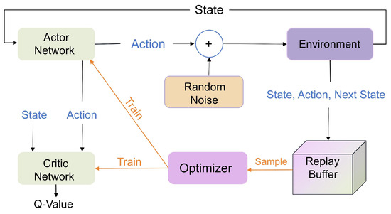
Figure 2.
The structure diagram of the DDPG algorithm.
The critic network is employed in RL to assess the value function of a given state–action pair, denoted as . Throughout the training process, the objective of the critic network is to minimize the mean squared error of the Bellman equation. The aim of the critic network is to assess the value function for state–action pairs, denoted as , where represents the parameters of the critic network. The critic network adjusts its parameters by minimizing the following Bellman equation:
Here, represents the objective function of the critic network, indicating the mean squared error between the estimated value and the actual return. D denotes the experience replay buffer, signifies the immediate reward, and denotes the output of the critic network, representing the estimated action value. Additionally, represents the deterministic policy generated by the target network for the next state, and denotes the parameters of the target network.
In the DDPG, the value function for state–action pairs, denoted as , is represented by the critic network. This is defined according to the Bellman equation as follows:
Moreover, represents the experience replay buffer. The DDPG introduces an experience replay mechanism to decouple correlations in continuous trajectories, thereby enhancing the algorithm’s stability and sample efficiency.
To improve stability, the DDPG also incorporates target networks, including the target policy network and the target value function network . The parameters of these target networks are periodically updated through a soft update mechanism, defined as follows:
Here, is a small constant, where , used to control the magnitude of the updates. This soft update strategy contributes to the gradual adjustment of the target network parameters, promoting algorithmic stability.
4.2. Training Procedure of DDPG
The training process of the DDPG primarily consists of two steps: a policy update and value function update. The DDPG updates its policy network by maximizing the action-value function . The actor network undergoes updates by applying the chain rule to the expected return of the initial distribution J. The optimization objective is structured as follows:
The DDPG updates the value function network by minimizing the mean squared error between the value function network and the target value function network. The optimization objective is expressed as follows:
Following the definition of the action value, the current action value can be represented as follows:
It is important to highlight that in both the estimated and actual reward elements, the current action value proves to be more precise compared to the evaluation derived from the Q network. The modification of network parameters can be depicted as follows:
In the DDPG, the network is divided into two parts: the current time-step network () and the previous time-step network (). The current network is used for action execution and network updates, while the previous network is used to compute the action for the next time step. The update of the network depends on the action value, with the objective of maximizing the action value. Therefore, the corresponding update equation is as follows:
Furthermore, Gaussian noise is incorporated into the network output to regulate the exploration rate of the network. Thus, the network output can be described as follows:
where represents the variance of the Gaussian noise.
4.3. Velocity Tracking Control Strategy Based on DDPG
In this section, a velocity tracking optimization control strategy is proposed based on the DDPG algorithm. The overall algorithmic structure is illustrated in Figure 3. In this framework, the network is tasked with receiving the current system state s and generating the action a. The action controller, after passing through a Gaussian distribution and action constraints, exerts control over the injection speed of the IMM. The network Q is responsible for representing the action value, evaluating the quality of action selection. Figure 4 provides a detailed depiction of the structures of the and Q networks.
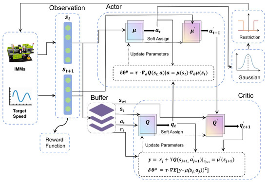
Figure 3.
The overall algorithmic structure proposed in this paper.
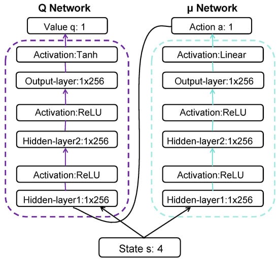
Figure 4.
Architecture of networks and Q.
The neural network framework adopts an end-to-end policy, mapping the observation space to the action space, akin to mapping desired output values to given parameters for the controller input. In the diagram, the forward propagation process of the actor neural network can be observed, transforming input states through a series of linear transformations and nonlinear activation functions to produce the output action. Specifically, in the experiments conducted in this paper, the network has two hidden layers, each with 256 nodes. The activation function for the hidden layers is ReLU, and the output layer is linear. In the architecture of the Q network, two hidden layers comprising 256 nodes each are established. ReLU serves as the activation function for these hidden layers, while the output layer employs a Tanh activation function. The DDPG involves both the actor and the critic neural networks collaborating. The actor network generates actions, while the critic evaluates the value associated with these actions. The training of this deep learning model typically involves using gradient descent methods to minimize a certain loss function, optimizing network parameters to generate better action policies and Q value estimates. The training process of the velocity tracking control strategy based on the DDPG is outlined in Algorithm 1.
| Algorithm 1 Training process of injection speed tracking control strategy via DDPG. |
|
5. Experimental Results
This section presents a series of simulation experiments conducted to confirm the feasibility and effectiveness of the proposed algorithm. The primary focus was on assessing the tracking control performance of the injection speed in the IMM using the DDPG optimal feedback controller developed. Initially, the RL model was trained based on the provided target state trajectory to acquire and produce optimal control policies. This enabled the achievement of tracking control for the desired injection speed trajectory within the specified time frame. Secondly, in the experimental section, we extensively discussed and analyzed the impact of hyperparameter tuning on the experimental results during the algorithm training process. Finally, we compared the experimental results of the proposed control strategy algorithm with the traditional PID control algorithm, further confirming the superiority of our proposed method. Throughout the entire experimental process, all the simulations were conducted in the Matlab R2023b simulation environment. Table 1 presents the pertinent characteristic parameters of the IMM filling model examined in this paper.

Table 1.
Main parameter settings.
5.1. Validation of DDPG-Based Controller
In this subsection, we conducted tracking control experiments for different injection speed targets in the IMM. The primary objective was to thoroughly validate the feasibility and effectiveness of the controller based on the DDPG algorithm proposed in this paper.
Initially, we focused on tracking control simulation experiments for the first set of desired IMM injection speed targets . We defined a two-stage injection speed trajectory to implement the optimal tracking controller design based on the DDPG algorithm. The final numerical results are illustrated in Figure 5. From the simulation results in Figure 5, it is evident that as the DDPG algorithm training progresses, the learning and decision networks gradually learn the optimal control strategy. This ultimately leads to the rapid and accurate convergence of the injection speed output of the dynamic injection molding system to the target speed curve. During the optimal controller design process, the DDPG algorithm determines the control gains in each control policy iteration by iteratively reinforcing the action-value function in the RL framework. In Figure 6, we provide a scatter plot of the control action values. Figure 7 illustrates the convergence progression of the average reward curve throughout the training of the algorithm. From the result figures, it can be observed that in the initial training stage of the algorithm, the action values and rewards fluctuate significantly, possibly reflecting the initial uncertainty of the system to the environment and the continuous trial-and-error process of learning. However, as the training progresses, we observe that the action values and rewards gradually stabilize. After a period of learning, the system can adjust its action strategy to better adapt to the specific requirements of the IMM. This indicates that the evolution process of training is not only the result of reducing action value fluctuations but also reflects a better understanding of the task goals by the system.
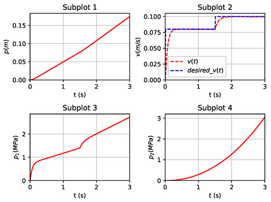
Figure 5.
State variables at tracking desired speed .
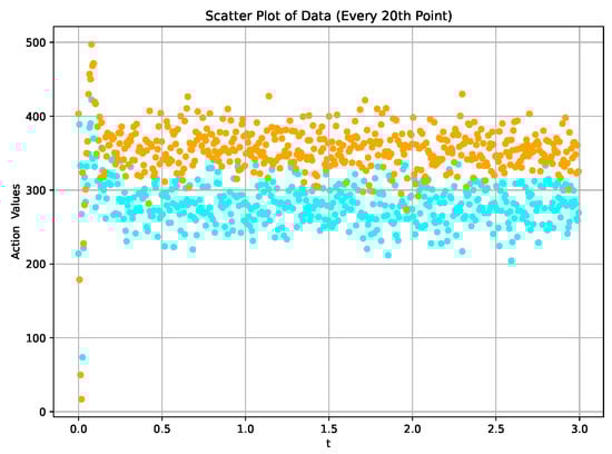
Figure 6.
The action values corresponding to the required speed .
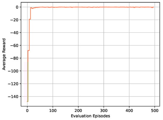
Figure 7.
The average reward curve corresponding to the required speed .
To further validate the effectiveness of the proposed controller based on the DDPG algorithm, we also conducted optimal tracking control simulation experiments for the given three-stage injection speed curves. The corresponding numerical results are shown in Figure 8, Figure 9 and Figure 10. Similar to the results of the two-stage injection speed trajectory tracking, as the DDPG algorithm training progresses, the learning and decision networks gradually learn the optimal control strategy. This ultimately leads to the rapid and accurate convergence of the injection speed output of the system to the target speed curve. The simulation results also affirm the effectiveness of the controller designed through the DDPG algorithm. Furthermore, we conducted optimal tracking control simulation experiments for four-stage injection speed curves, and the corresponding numerical results are presented in Figure 11, Figure 12 and Figure 13. Similar to the results of the two-stage and three-stage injection speed trajectory tracking, the simulation results also confirm the effectiveness of the controller designed through the DDPG algorithm.
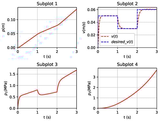
Figure 8.
State variables at tracking desired speed .
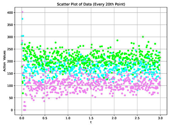
Figure 9.
The action values corresponding to the required speed .
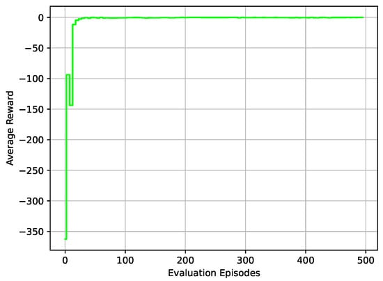
Figure 10.
The average reward corresponding to the required speed .
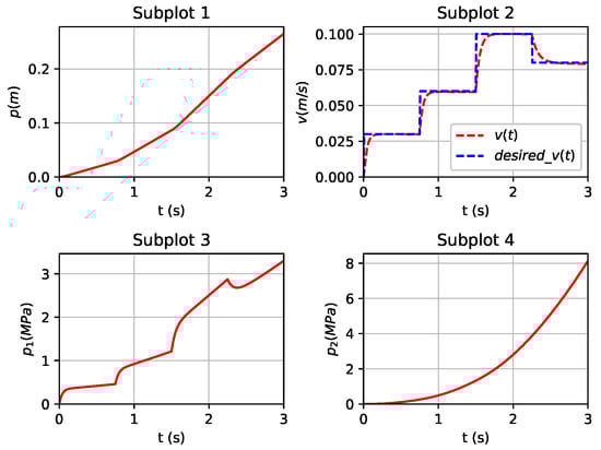
Figure 11.
State variables at tracking desired speed .
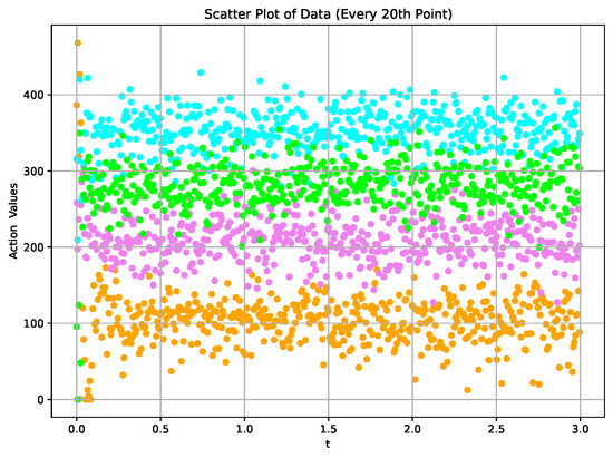
Figure 12.
The action values corresponding to the required speed .
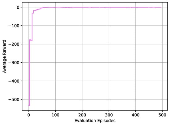
Figure 13.
The average reward corresponding to the required speed .
Additionally, during the experimental process, it was demonstrated that with the extension of the training time of the reinforcement learning algorithm, the system’s error in reaching the target speed gradually decreased. Through longer training times, the model or system could more effectively adapt to the environment, learn more accurate control strategies, and exhibit more stable and accurate performance when achieving the target speed.
5.2. Hyperparameter Tuning
During the experimental process, we conducted a study on the hyperparameters of the algorithm, testing and analyzing the impact of different hyperparameter settings on the experimental results. The specific analysis of the experimental results is presented below.
5.2.1. Gaussian Noise in Action Space
During training, Gaussian noise is incorporated into the output actions of the network. This assists in introducing a degree of randomness into the training procedure. This comprehensive learning of the environment model encourages the agent to explore the environment more effectively, enhancing the algorithm’s robustness and generalization. The variance plays a pivotal role in defining the extent of the exploration space. Altering the values of different variances results in varying convergence speeds during training. When exceeds 0.3, the network fails to converge within the training period, leading to training instability. As shown in Figure 14, when is within the range of 0.02–0.30, the network exhibits good stability. Larger values of lead to slower convergence.
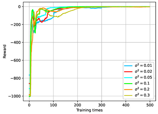
Figure 14.
Convergence curve of reward under different variances of Gaussian noise .
5.2.2. Discount Factor in the Reward Function
The discount factor in the reward function has a significant impact on DRL algorithms. When approaches 1, the diminishing effect of future rewards is reduced, and the agent pays more attention to long-term rewards. This inclination encourages the agent to make decisions that lead to higher cumulative rewards in the long run. Conversely, when approaches 0, the diminishing effect of future rewards is enhanced, and the agent focuses more on immediate rewards. This tendency leads the agent to make decisions that result in immediately higher rewards, without much consideration for long-term consequences. In the context of the speed tracking task, the impact of different discount factors on reward convergence is investigated. As shown in Figure 15, the convergence curves of rewards under different discount factors indicate that the average reward does not vary significantly as increases from 0.1 to 0.999. The findings indicate that the network demonstrates a strong tolerance for a wide range of values.
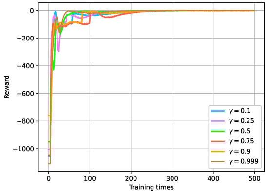
Figure 15.
Convergence curve of reward under different discount factors of reward function.
5.2.3. Soft Update Parameter for Updating Target Network
The parameter is responsible for controlling the proportion of new weights introduced during updates. When is small, the introduction of new weights to the main network is gradual, resulting in smoother updates. On the other hand, when is large, updates occur more rapidly. Selecting an appropriate value often requires experimentation and adjustment during the training process. As depicted in Figure 16, when increases from 0.005 to 0.5, the convergence of the reward curve becomes slower with the increasing . However, the algorithm still effectively tracks the expected speed curve. This observation suggests that a careful choice of is crucial for achieving a balance between stability and convergence speed.
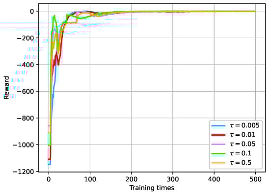
Figure 16.
Convergence curve of rewards under different soft update parameters for updating target networks.
5.2.4. Batch Size for Training
The batch size, representing the number of samples randomly drawn from the experience replay buffer during each model parameter update, is another crucial hyperparameter in this experiment. To optimize the replay buffer, experiments were conducted using five different batch sizes within the range of [10–500]. As shown in Figure 17, the experimental results indicate that as the batch size for training increases, the convergence becomes faster, leading to improved controller performance.
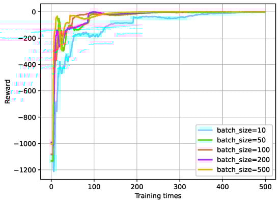
Figure 17.
Convergence curve of rewards under different sample batch sizes used in training.
5.2.5. Learning Rate
For the DDPG, a deep reinforcement learning algorithm suitable for continuous action spaces, a small learning rate is commonly chosen. As illustrated in Figure 18, the comparison of the experimental results reveals that a smaller learning rate results in smaller update magnitudes and a potentially slower convergence of rewards. However, a smaller learning rate leads to a more stable model that can better adapt to noise and variations, resulting in a more effective tracking of the expected speed curve.
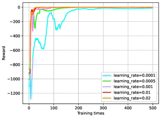
Figure 18.
Convergence curve of rewards under different learning rates.
5.3. Compared with PID Method
To further validate the performance of the proposed DDPG-based RL controller for the speed tracking task in the system, more experiments were conducted for comparing our proposed control algorithm with the widely used PID control method, as well as the Ziegler–Nichols and Cohen–Coon tuning methods. In the field of speed tracking control for IMMs, PID control is widely applied due to its simplicity and intuitive design. Ziegler–Nichols (ZN) and Cohen–Coon (C-C) are two common methods for PID parameter tuning, designed to optimize control performance. However, these traditional control methods demonstrate significant limitations when applied to complex, high-dimensional dynamic systems.
In the comparative experiments, the control performance of the PID (including the ZN and C-C methods) is compared with that of the proposed DDPG-based controller in tracking the injection speed profile. The results, as shown in Figure 19, reveal that in the three-stage injection speed profile tracking task, the PID-based control schemes exhibited noticeable oscillations at certain points. This issue was especially evident with the ZN and C-C methods, which struggled to prevent significant overshoot and response instability. In contrast, the DDPG-based controller demonstrated superior stability and adaptability to dynamic changes. The DDPG controller was capable of adjusting its strategy in real time, resulting in smoother speed profile tracking with minimal oscillation and overshoot. Therefore, the experimental results highlight the clear advantages of the DDPG controller in addressing the high-dimensional, nonlinear dynamic task of IMM speed tracking. Compared to the Ziegler–Nichols and Cohen–Coon methods, the DDPG not only improved control accuracy but also enhanced system robustness and stability. Particularly when handling complex nonlinear systems, the DDPG provides a more forward-looking and efficient control solution, surpassing the limitations of traditional PID methods.
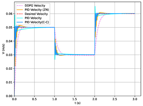
Figure 19.
Under the PID method, the state variable tracks the trajectory of the required speed .
6. Conclusions
This paper focuses on the nonlinear hydraulic servo control system within a standard IMM, presenting the design of an efficient optimal controller based on the DDPG algorithm. The primary objective of the controller is to achieve rapid tracking control of the injection speed within a predefined time frame. Employing the framework of deep reinforcement learning algorithms, we constructed a customized MDP model for the control of the injection molding speed. This model meticulously defines the state space, action space, and reward function. Expanding upon this model, we established an injection speed tracking control strategy based on the DDPG. This approach enables the controller to learn the optimal control policy through interaction with the environment. To validate the feasibility and effectiveness of the proposed method, we conducted extensive experimental simulations. The results demonstrate that the suggested algorithm can adeptly and efficiently track the desired injection speed. In contrast to the traditional PID method, the DDPG-based approach requires no expert tuning, resulting in smoother speed profiles and smaller speed errors. The methodology proposed in this paper exhibits promising applications and can be extended to address optimal control challenges in other intricate injection molding industrial processes. Furthermore, its applicability extends to analogous nonlinear optimal control issues in discrete manufacturing processes. Although the method proposed in this work is very effective, it should be also noted that there is still much room for improvement in the future. For example, the exploration of more offline DRL algorithms can be also pursued in future work. Moreover, more injection molding process production factors need to be taken into account. For example, in the injection molding process, the projected area and the mass of the part to be injected significantly affect the injection pressure, injection speed, cooling time, cycle time, and mold design complexity. Larger projected areas and heavier parts typically require higher injection pressure and speed, extended cooling times, increased material usage, and more complex mold designs. These factors also impact production efficiency and costs. Therefore, during design and production, these aspects should also be carefully considered to optimize the molding process and ensure the final product quality. In addition, the size of the clamping force also impacts equipment selection and energy consumption. Properly determining the clamping force is essential not only for ensuring part quality but also for optimizing production efficiency and cost-effectiveness.
Author Contributions
Conceptualization, W.Z.; Methodology, Z.R., P.T. and W.Z.; Validation, P.T.; Formal analysis, Z.R., P.T. and W.Z.; Resources, B.Z.; Data curation, B.Z.; Writing—original draft, Z.R.; Writing—review & editing, Z.R.; Visualization, P.T.; Supervision, B.Z.; Project administration, Z.R. All authors have read and agreed to the published version of the manuscript.
Funding
Guang-dong Basic and Applied Basic Research Foundation (2024A1515011768), National Natural Science Foundation of China (62073088).
Data Availability Statement
Data available on request from the authors.
Acknowledgments
This work was supported in part by the Guang-dong Basic and Applied Basic Research Foundation (2024A1515011768) and the National Natural Science Foundation of China (62073088).
Conflicts of Interest
The authors declare no conflicts of interest.
References
- Fernandes, C.; Pontes, A.J.; Viana, J.C.; Gaspar-Cunha, A. Modeling and Optimization of the Injection-Molding Process: A Review. Adv. Polym. Technol. 2018, 37, 429–449. [Google Scholar] [CrossRef]
- Gao, H.; Zhang, Y.; Zhou, X.; Li, D. Intelligent methods for the process parameter determination of plastic injection molding. Front. Mech. Eng. 2018, 13, 85–95. [Google Scholar] [CrossRef]
- Fu, H.; Xu, H.; Liu, Y.; Yang, Z.; Kormakov, S.; Wu, D.; Sun, J. Overview of injection molding technology for processing polymers and their composites. ES Mater. Manuf. 2020, 8, 3–23. [Google Scholar] [CrossRef]
- Cho, Y.; Cho, H.; Lee, C.O. Optimal open-loop control of the mould filling process for injection moulding machines. Optim. Control Appl. Methods 1983, 4, 1–12. [Google Scholar] [CrossRef]
- Havlicsek, H.; Alleyne, A. Nonlinear control of an electrohydraulic injection molding machine via iterative adaptive learning. IEEE/ASME Trans. Mechatron. 1999, 4, 312–323. [Google Scholar] [CrossRef]
- Dubay, R. Self-optimizing MPC of melt temperature in injection moulding. ISA Trans. 2002, 41, 81–94. [Google Scholar] [CrossRef]
- Huang, S.; Tan, K.K.; Lee, T.H. Neural-network-based predictive learning control of ram velocity in injection molding. IEEE Trans. Syst. Man Cybern. Part C (Appl. Rev.) 2004, 34, 363–368. [Google Scholar] [CrossRef]
- Yao, K.; Gao, F. Optimal start-up control of injection molding barrel temperature. Polym. Eng. Sci. 2007, 47, 254–261. [Google Scholar] [CrossRef]
- Chen, W.C.; Tai, P.H.; Wang, M.W.; Deng, W.J.; Chen, C.T. A neural network-based approach for dynamic quality prediction in a plastic injection molding process. Expert Syst. Appl. 2008, 35, 843–849. [Google Scholar] [CrossRef]
- Xia, W.; Luo, B.; Liao, X. An enhanced optimization approach based on Gaussian process surrogate model for process control in injection molding. Int. J. Adv. Manuf. Technol. 2011, 56, 929–942. [Google Scholar] [CrossRef]
- Wang, Y.; Jin, Q.; Zhang, R. Improved fuzzy PID controller design using predictive functional control structure. ISA Trans. 2017, 71, 354–363. [Google Scholar] [CrossRef] [PubMed]
- Yang, A.; Guo, W.; Han, T.; Zhao, C.; Zhou, H.; Cai, J. Feedback Control of Injection Rate of the Injection Molding Machine Based on PID Improved by Unsaturated Integral. Shock Vib. 2021, 2021, 9960021. [Google Scholar] [CrossRef]
- Farahani, S.; Khade, V.; Basu, S.; Pilla, S. A data-driven predictive maintenance framework for injection molding process. J. Manuf. Process. 2022, 80, 887–897. [Google Scholar] [CrossRef]
- Xiao, H.; Meng, Q.X.; Lai, X.Z.; Yan, Z.; Zhao, S.Y.; Wu, M. Design and trajectory tracking control of a novel pneumatic bellows actuator. Nonlinear Dyn. 2023, 111, 3173–3190. [Google Scholar] [CrossRef]
- Ruan, Y.; Gao, H.; Li, D. Improving the Consistency of Injection Molding Products by Intelligent Temperature Compensation Control. Adv. Polym. Technol. 2019, 2019, 1591204. [Google Scholar] [CrossRef]
- Stemmler, S.; Vukovic, M.; Ay, M.; Heinisch, J.; Lockner, Y.; Abel, D.; Hopmann, C. Quality Control in Injection Molding based on Norm-optimal Iterative Learning Cavity Pressure Control. IFAC-PapersOnLine 2020, 53, 10380–10387. [Google Scholar] [CrossRef]
- Xu, J.; Ren, Z.; Xie, S.; Wang, Y.; Wang, J. Deep learning-based optimal tracking control of flow front position in an injection molding machine. Optim. Control Appl. Methods 2023, 44, 1376–1393. [Google Scholar] [CrossRef]
- Ren, Z.; Wu, G.; Wu, Z.; Xie, S. Hybrid dynamic optimal tracking control of hydraulic cylinder speed in injection molding industry process. J. Ind. Manag. Optim. 2023, 19, 5209–5229. [Google Scholar] [CrossRef]
- Wu, G.; Ren, Z.; Li, J.; Wu, Z. Optimal Robust Tracking Control of Injection Velocity in an Injection Molding Machine. Mathematics 2023, 11, 2619. [Google Scholar] [CrossRef]
- Ren, Z.; Lin, J.; Wu, Z.; Xie, S. Dynamic optimal control of flow front position in injection molding process: A control parameterization-based method. J. Process Control 2023, 132, 103125. [Google Scholar] [CrossRef]
- Tan, K.; Tang, J. Learning-enhanced PI control of ram velocity in injection molding machines. Eng. Appl. Artif. Intell. 2002, 15, 65–72. [Google Scholar] [CrossRef]
- Tian, Y.C.; Gao, F. Injection velocity control of thermoplastic injection molding via a double controller scheme. Ind. Eng. Chem. Res. 1999, 38, 3396–3406. [Google Scholar] [CrossRef][Green Version]
- Lillicrap, T.P.; Hunt, J.J.; Pritzel, A.; Heess, N.; Erez, T.; Tassa, Y.; Silver, D.; Wierstra, D. Continuous control with deep reinforcement learning. arXiv 2015, arXiv:1509.02971. [Google Scholar]
- Zamfirache, I.A.; Precup, R.E.; Roman, R.C.; Petriu, E.M. Reinforcement Learning-based control using Q-learning and gravitational search algorithm with experimental validation on a nonlinear servo system. Inf. Sci. 2022, 583, 99–120. [Google Scholar] [CrossRef]
- Zamfirache, I.A.; Precup, R.E.; Roman, R.C.; Petriu, E.M. Policy iteration reinforcement learning-based control using a grey wolf optimizer algorithm. Inf. Sci. 2022, 585, 162–175. [Google Scholar] [CrossRef]
- Wang, N.; Gao, Y.; Zhao, H.; Ahn, C.K. Reinforcement learning-based optimal tracking control of an unknown unmanned surface vehicle. IEEE Trans. Neural Netw. Learn. Syst. 2020, 32, 3034–3045. [Google Scholar] [CrossRef]
- Shuprajhaa, T.; Sujit, S.K.; Srinivasan, K. Reinforcement learning based adaptive PID controller design for control of linear/nonlinear unstable processes. Appl. Soft Comput. 2022, 128, 109450. [Google Scholar] [CrossRef]
- Sun, Y.; Ran, X.; Zhang, G.; Wang, X.; Xu, H. AUV path following controlled by modified Deep Deterministic Policy Gradient. Ocean Eng. 2020, 210, 107360. [Google Scholar] [CrossRef]
- Bilal, H.; Yin, B.; Aslam, M.S.; Anjum, Z.; Rohra, A.; Wang, Y. A practical study of active disturbance rejection control for rotary flexible joint robot manipulator. Soft Comput. 2023, 27, 4987–5001. [Google Scholar] [CrossRef]
- Xu, L.; Yuehui, J.; Yu, S.; Junjie, L.; Qiang, G. Modified deep deterministic policy gradient based on active disturbance rejection control for hypersonic vehicles. Neural Comput. Appl. 2024, 36, 4071–4081. [Google Scholar] [CrossRef]
- Ning, L.; Zhou, M.; Hou, Z.; Goverde, R.M.; Wang, F.Y.; Dong, H. Deep deterministic policy gradient for high-speed train trajectory optimization. IEEE Trans. Intell. Transp. Syst. 2021, 23, 11562–11574. [Google Scholar] [CrossRef]
- Yan, R.; Jiang, R.; Jia, B.; Huang, J.; Yang, D. Hybrid car-following strategy based on deep deterministic policy gradient and cooperative adaptive cruise control. IEEE Trans. Autom. Sci. Eng. 2021, 19, 2816–2824. [Google Scholar] [CrossRef]
- Wang, N.; Gao, Y.; Yang, C.; Zhang, X. Reinforcement learning-based finite-time tracking control of an unknown unmanned surface vehicle with input constraints. Neurocomputing 2022, 484, 26–37. [Google Scholar] [CrossRef]
- Hao, G.; Fu, Z.; Feng, X.; Gong, Z.; Chen, P.; Wang, D.; Wang, W.; Si, Y. A deep deterministic policy gradient approach for vehicle speed tracking control with a robotic driver. IEEE Trans. Autom. Sci. Eng. 2021, 19, 2514–2525. [Google Scholar] [CrossRef]
- Guo, H.; Ren, Z.; Lai, J.; Wu, Z.; Xie, S. Optimal navigation forAGVs: A soft actor–critic-based reinforcement learning approach with composite auxiliary rewards. Eng. Appl. Artif. Intell. 2023, 124, 106613. [Google Scholar] [CrossRef]
- Ma, Y.; Zhu, W.; Benton, M.G.; Romagnoli, J. Continuous control of a polymerization system with deep reinforcement learning. J. Process Control 2019, 75, 40–47. [Google Scholar] [CrossRef]
- Qiu, C.; Hu, Y.; Chen, Y.; Zeng, B. Deep deterministic policy gradient (DDPG)-based energy harvesting wireless communications. IEEE Internet Things J. 2019, 6, 8577–8588. [Google Scholar] [CrossRef]
- Joshi, T.; Makker, S.; Kodamana, H.; Kandath, H. Twin actor twin delayed deep deterministic policy gradient (TATD3) learning for batch process control. Comput. Chem. Eng. 2021, 155, 107527. [Google Scholar] [CrossRef]
- Wei, Z.; Quan, Z.; Wu, J.; Li, Y.; Pou, J.; Zhong, H. Deep deterministic policy gradient-DRL enabled multiphysics-constrained fast charging of lithium-ion battery. IEEE Trans. Ind. Electron. 2021, 69, 2588–2598. [Google Scholar] [CrossRef]
- Yoo, H.; Kim, B.; Kim, J.W.; Lee, J.H. Reinforcement learning based optimal control of batch processes using Monte-Carlo deep deterministic policy gradient with phase segmentation. Comput. Chem. Eng. 2021, 144, 107133. [Google Scholar] [CrossRef]
- Watkins, C.J.; Dayan, P. Q-learning. Mach. Learn. 1992, 8, 279–292. [Google Scholar] [CrossRef]


Disclaimer/Publisher’s Note: The statements, opinions and data contained in all publications are solely those of the individual author(s) and contributor(s) and not of MDPI and/or the editor(s). MDPI and/or the editor(s) disclaim responsibility for any injury to people or property resulting from any ideas, methods, instructions or products referred to in the content. |
© 2024 by the authors. Licensee MDPI, Basel, Switzerland. This article is an open access article distributed under the terms and conditions of the Creative Commons Attribution (CC BY) license (https://creativecommons.org/licenses/by/4.0/).