Abstract
Currently, key factors hindering application of steer-by-wire systems are their inadequate safety and reliability, which are significant criteria for evaluating automotive active safety. Based on the steer-by-wire platform, a dual-redundant steering motor control system is proposed, featuring dual three-phase permanent magnet synchronous motors as execution motors, achieving redundancy from hardware. A torque vector-space-decoupling control method is introduced for these motors to ensure balanced and stable torque output. Upon a fault, fault-tolerant measures are taken by disconnecting power supply to the affected motor, which, despite reducing system functionality, allows for normal steering control. This research starts with modeling the dual three-phase motors to construct a simulation model. It then proceeds with hardware-in-the-loop testing integrated with the dual-redundancy steer-by-wire control system, conducting tests under dual-lane-change trajectory conditions. Finally, a steering system fault is simulated to assess fault handling and functional degradation. These experiments confirmed that the proposed method enabled balanced torque output from the dual three-phase motors in the redundant steering control and facilitated fault-tolerant processing post fault, ensuring the vehicle’s steering functions were maintained.
1. Introduction
Steer-by-Wire (SBW) is a key technology enabling vehicles to achieve autonomous driving, complete automatic obstacle avoidance, and path tracking. The performance of SBW systems directly influences automotive active safety and the driver’s experience, positioning it as one of the research hotspots in the automotive active safety domain. However, theoretical and key technological research on SBW systems is still immature, particularly concerning adaptability and robustness of the steering system under complex conditions and how to handle failures within the steering system, which severely hinders their large-scale application. As an integral component of the vehicle chassis, the SBW system is central to automotive active safety; its safety and reliability are particularly important, determining the vehicle’s ability to drive safely.
Currently, there are two main research directions for SBW systems: dual-motor control strategies and dual three-phase motor control strategies. Both implement redundancy fault tolerance for the steering system essentially through hardware redundancy, thereby enhancing the system’s safety and reliability. The dual-motor control strategy is mainstream due to its simpler implementation. Huang and Zheng proposed a redundant mechanism with dual motors and dual controllers for the steering gear to improve system safety [1,2]. Yao suggested using a synchronous controller for motor torque compensation and closed-loop control for each motor separately [3]. Lin Hui, Zhou Yuanjun, and Ma Ruiqing presented a method where target current output, based on a velocity closed loop, is equally divided among current closed loops [4,5,6]. Sohel and Mohammad integrated vehicle safety into steering design, advocating for fault detection, isolation, and angle detection in dual-motor steering systems to enhance safety [7,8,9]. Mi Junnan introduced a current-balancing redundancy control strategy to equally distribute torque current of two motors and presented a control method with reduced complexity [10]. In the field of dual three-phase motor control, development has been relatively slow due to factors such as magnetic coupling and harmonic currents. Wang Xueqing developed a model of a six-phase stationary coordinate system of dual three-phase motors for direct torque control using space vector decoupling [11]. Bojoi transformed dual three-phase motors into two three-phase motors and then applied sinusoidal pulse-width modulation, enhancing bus voltage utilization by injecting zero-sequence components [12]. A dual decoupling modulation strategy was proposed for dual three-phase motors. Bhattacharya designed a configuration where two sets of three-phase windings are split in the stator slots to avoid magnetic field coupling between the windings [13]. Dordevic recommended a comprehensive solution strategy that combines design of cascaded H-bridge multilevel converters with dual three-phase motors and applies sinusoidal pulse-width modulation to multiphase multilevel drive systems [14,15]. Harmonic injection into multiphase motors was used to improve torque output capacity, and a hysteresis controller was employed in the coordinate system plane of the dual three-phase motors to address suppression of harmonic currents [16]. In recent years, model predictive control has been increasingly applied to the control of multiphase motors due to its dynamic and rapid response capabilities [17,18,19,20].
This paper introduces a torque vector-space-decoupling control method for dual three-phase motors in SBW systems, adopting these motors as the steering executive. By decoupling in the torque vector space, the method ensures balanced and stable torque output from steering motors, and fault-tolerant processing is executed after a fault occurs to ensure normal execution of the steering functions. Finally, the control method is validated through hardware-in-the-loop testing.
2. SBW System Design
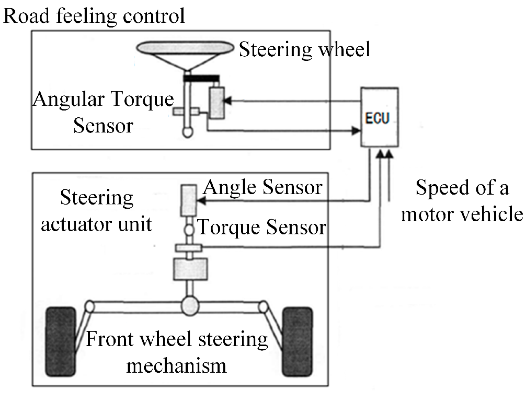
The SBW system, as outlined in Figure 1, integrates a steering execution unit, a road sense simulation unit, and an engine control unit (ECU). Unlike traditional electric power steering systems, SBW employs a road-sense motor and a steering executive motor to replace the mechanical linkage between the steering gear and the execution unit, enhancing the steering system’s adaptability and breaking free from the fixed transmission ratio of conventional steering systems. However, this innovation comes at the cost of reduced safety and reliability due to the absence of a mechanical linkage.

Figure 1.
Schematic diagram of the SBW system components.
2.1. Mathematical Model of the Steering Executive Unit
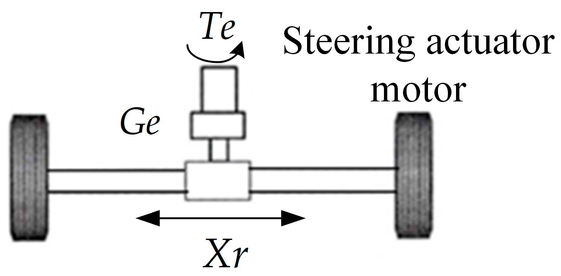
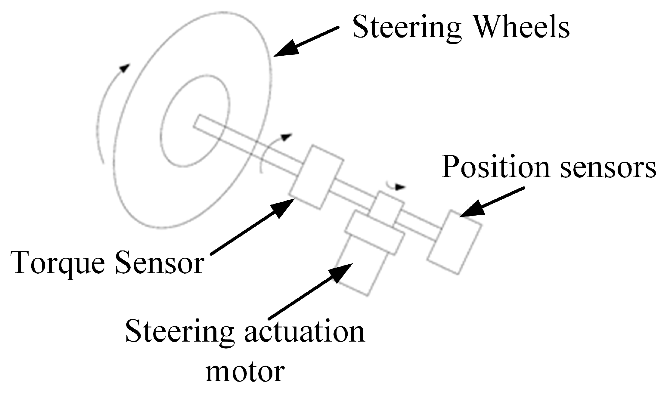
Figure 2 shows the vehicle steer-by-wire executive structure. The steering executive motor generates steering torque through differential drive to the wheels to realize vehicle steering functions. The dynamic balance equation of the steering actuator motor is:
where is electromagnetic torque of the steering executive motor; is motor moment of inertia; is torsional stiffness of the motor; is resistance of the motor; is angular displacement of the motor; is the pinion radius; is the motor reduction ratio; and is the rack displacement.
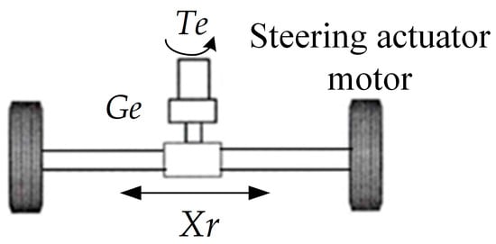
Figure 2.
Schematic diagram of the steering execution assembly structure. : Electromagnetic torque of the steering executive motor; : Motor reduction ratio; and : Rack displacement.
The rack and pinion module can be represented as:
In Equation (2), is quality of rack and pinion; , are torsional stiffness of the main pin of the left and right front wheels; is stiffness of the rack and pinion; is the damping coefficient of the rack and pinion; is positive efficiency of the rack and pinion; , are ratios of the rack and the left and right front wheels; and , are steering angles of the left and right front wheels of the car.
Motion analysis of steering for the left front wheel can be articulated by the equation:
where is steering torque acting on the left front wheel, is inertia of the left front wheel around the main pin, and is the damping coefficient of the left front wheel around the main pin.
Similarly, a description of the movement of steering for the right front wheel around the kingpin can be obtained.
2.2. Mathematical Model of Steering Wheel
As shown in Figure 3, when a driver manipulates the steering wheel, the steering wheel will overcome damping of the steering column and cause the steering column to twist. According to Newton’s Second Law, the steering wheel and steering column are simplified; regarded as a whole, friction torque of the steering wheel assembly is ignored; and finally, the dynamic balance equation of the vehicle steering wheel is obtained:
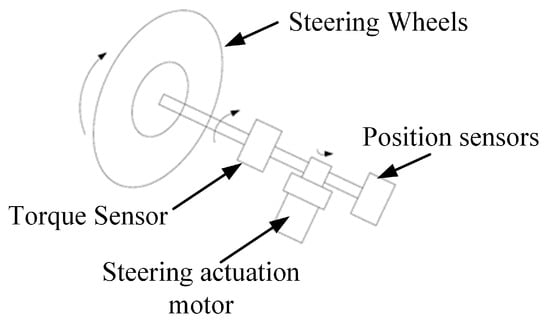
Figure 3.
Structural diagram of steering wheel assembly.
In Equation (4), is steering wheel angle, is motor angle, is steering wheel moment of inertia, is the damping coefficient of the steering column, is input torque from the driver, is torsional stiffness of the steering column, is the damping coefficient of the motor, and is transmission ratio from the motor to the steering column.
The road-sense simulation unit includes a road induction machine and a reducer. It mainly simulates positive-return torque according to signal output by the ECU and feeds it back to the driver’s road sense, that is, to the steering wheel feedback torque. Its kinematics balance equation is as follows:
In Equation (5), is rotational inertia of the road-sense motor, is motor angle, and is electromagnetic torque of the road-sense motor.
In order to facilitate simulation analysis, a model of the road induction machine can be simplified into a DC motor. The electrical balance equation of Kirchhoff’s Law is as follows:
where is the coefficient of reverse electromotive force, U is motor terminal voltage, R is motor armature resistance, L is motor armature inductance, and I is motor armature current.
3. Dual Three-Phase Motor Torque Vector Space Decoupling
In order to solve the problem of the safety and reliability of a steering system being reduced due to cancellation of the mechanical connecting rod in SBW, a dual three-phase permanent magnet synchronous motor as shown in Figure 4 is used as the steering execution motor. When one set of windings fails, the other set of windings continues to work to complete the steering execution. In the figure, A~C are the first set of motor windings, and D~F are the second set of motor windings.
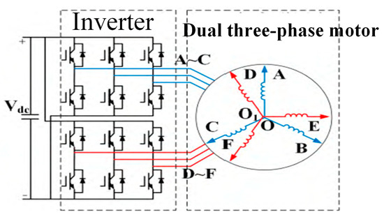
Figure 4.
Structural diagram of dual three-phase permanent magnet synchronous motor, A~C and D~F are motor windings, is the power supply and , are the two sets of motor winding neutral point.
3.1. Design of Dual-Redundancy SBW System
The dual-redundancy SBW system with higher safety, stability and reliability is obtained by applying redundancy theory to the SBW system, as shown in Figure 5.
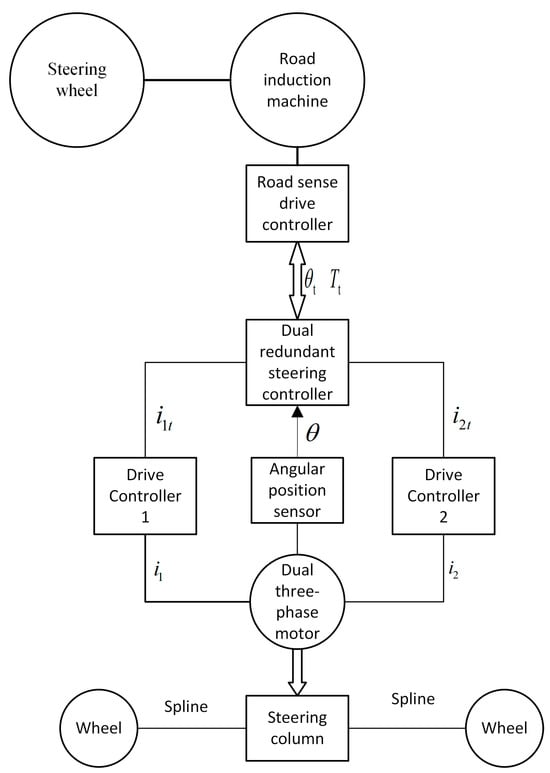
Figure 5.
Dual-redundancy SBW system. : Signal from road-sense drive controller. , : Torque current-control signals. , : Torque current signals.
In Figure 5, the dual-redundancy steer-by-wire controller, drive controllers 1 and 2 and the road sense drive controller (which has two sets of control loops identical to the drive controllers) together form the controller group of the dual-redundancy steer-by-wire control system. The dual-redundancy steering controller receives a road-sensing motor angle from the road-sense drive controller, calculates a target angle for the dual three-phase motors with the rotation ratio coefficient, and sends torque current-control signals and to drive controllers 1 and 2; when the drive controllers receive these signals, they generate torque currents and to jointly drive the dual three-phase motors to rotate to a target position; and in response the dual three-phase motors rotate to the target position. Meanwhile, angle and feedback currents of the dual three-phase motors’ torque currents and are fed to the dual redundant steering controller for calculating angle currents of the road-sensing driver and a target angle to control the road-sensing motors, generating a road-sensing torque for the steering wheel of the vehicle and a real-time angle for the steering wheel.
When the dual redundant SBW system works normally, the steering controller simultaneously sends control signals to drive controller 1 and drive controller 2, and the drive controllers generate torque currents to drive two sets of windings in the dual three-phase motors, to generate torque and jointly perform the steering function. Therefore, this paper proposes a torque vector-space-decoupling control method for dual three-phase motors. After a set of motor windings in one of the dual three-phase motors fails within the steering execution system, the function-reduction steering system performs fault-tolerant processing, the control signal and power supply of the control loop where failed windings are located are cut off, and the loop with fault-free motor winding continues to work, so that the steering control system can continue to perform normal steering functions.
The above SBW system has working characteristics of redundant functions with two sets of circuit-sensing feedback execution loops and steering-execution control loops that are independent of each other. After any set of circuits fails, the corresponding devices of the other set of circuits continue normal steering functions and send fault codes to inform both driver and engineers of the causes of the failure and remind them to repair the faults as soon as possible, so as to restore the reliability and safety of the system.
The torque vector-space-decoupling control mainly includes redundant control of the dual three-phase SBW system, torque-balanced output of the dual three-phase motors, and fault-tolerant control of the dual three-phase motors reduced-order system.
3.2. Dual Three-Phase SBW System Redundant Control
Redundant control of the dual-redundancy three-phase steer-by-wire system is shown in Figure 6.

Figure 6.
Dual three-phase SBW system redundant control. A: Dual three-phase SBW acceleration module. P: Regulators for speed loop and current loop. V: Torque-balancing output module for dual three-phase motors. f1, f2: Space–vector pulse-width modulation (SVPWM) modules. M: Dual three-phase permanent magnet synchronous motors. R: Steering executive mechanism. C1, C2, C3: System downgrade signals. : Target steering angle. : Actual steering angle. : Target rotational speed of the steering executive motor. : Actual rotational speed. : Actual motor current. : Target torque output current. , : Current signals. , : Drive modules.
In Figure 6, the dual-redundancy steer-by-wire control system transmits a target steering angle and the actual current steering angle of the steering executive motor to the dual three-phase SBW acceleration module A. This module calculates a target rotational speed for the steering executive motor. The actual rotational speed and the actual motor current are then input into the regulators (P) for both the speed loop and the current loop, which compute a target torque output current . The torque-balancing module V receives this data and balances the torque output, generating current signals and for the two sets of windings in the dual three-phase motors. These current signals are then processed by drive modules and , which respectively output torque currents for each set of windings in the dual three-phase motors. Torque is subsequently applied to the motors, controlling operations of the steering executive mechanism R.
The algorithm for the dual three-phase steer-by-wire acceleration module A is:
In Equations (7) and (8), is the difference between a target angle and the actual angle of the dual three-phase steering executive motor, is the maximum-permissible angular difference of the operating mode, is the speed of the constant-speed mode (its value is a constant), and is the S-shaped acceleration mode speed. The algorithm dictates that the output speed is zero when the difference between the target and actual angles of the steering executive motor is zero. If this difference is greater than zero but less than the maximum-allowable angle, the system transitions to constant-speed mode. Beyond the maximum-allowable angle, the system switches to an S-shaped acceleration mode.
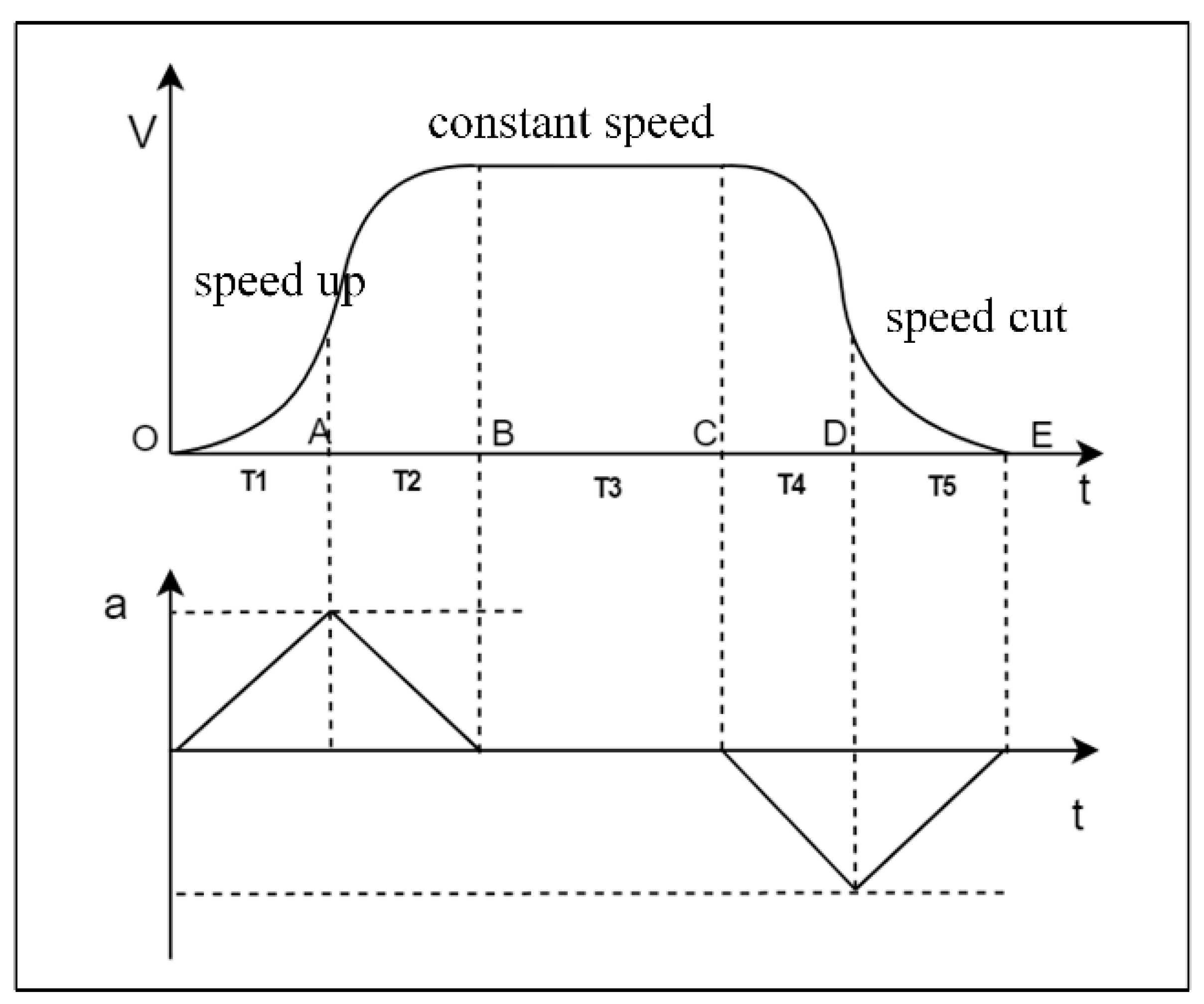
In Figure 7, signifies the initial acceleration phase, the deceleration phase, the constant velocity phase, and and the acceleration and deceleration phases, respectively. The acceleration curves start and end at zero, with equal slopes, and , indicating that the rates of change in acceleration (J) are equivalent but directed oppositely.
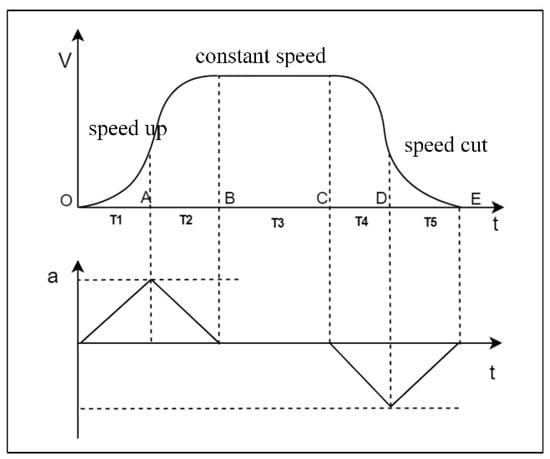
Figure 7.
S-shaped acceleration curve. T1: Initial acceleration phase. T2: Deceleration phase. T3: Constant-velocity phase. T4: Acceleration phase. T5: Deceleration phase. : Motor speed. : Time. : Starting point. , , , , : Motor operating mode switching time point. : Max. acceleration.
Acceleration phase:
Deceleration phase:
The total displacement of the acceleration phase:
where is initial speed, is acceleration curve running time, is real-time speed of the motor, and and denote displacement of the motor during acceleration and deceleration phases, respectively.
Similarly, the algorithm for the deceleration phase can be obtained.
Eventually, the following formula can be obtained:
For these calculations, .
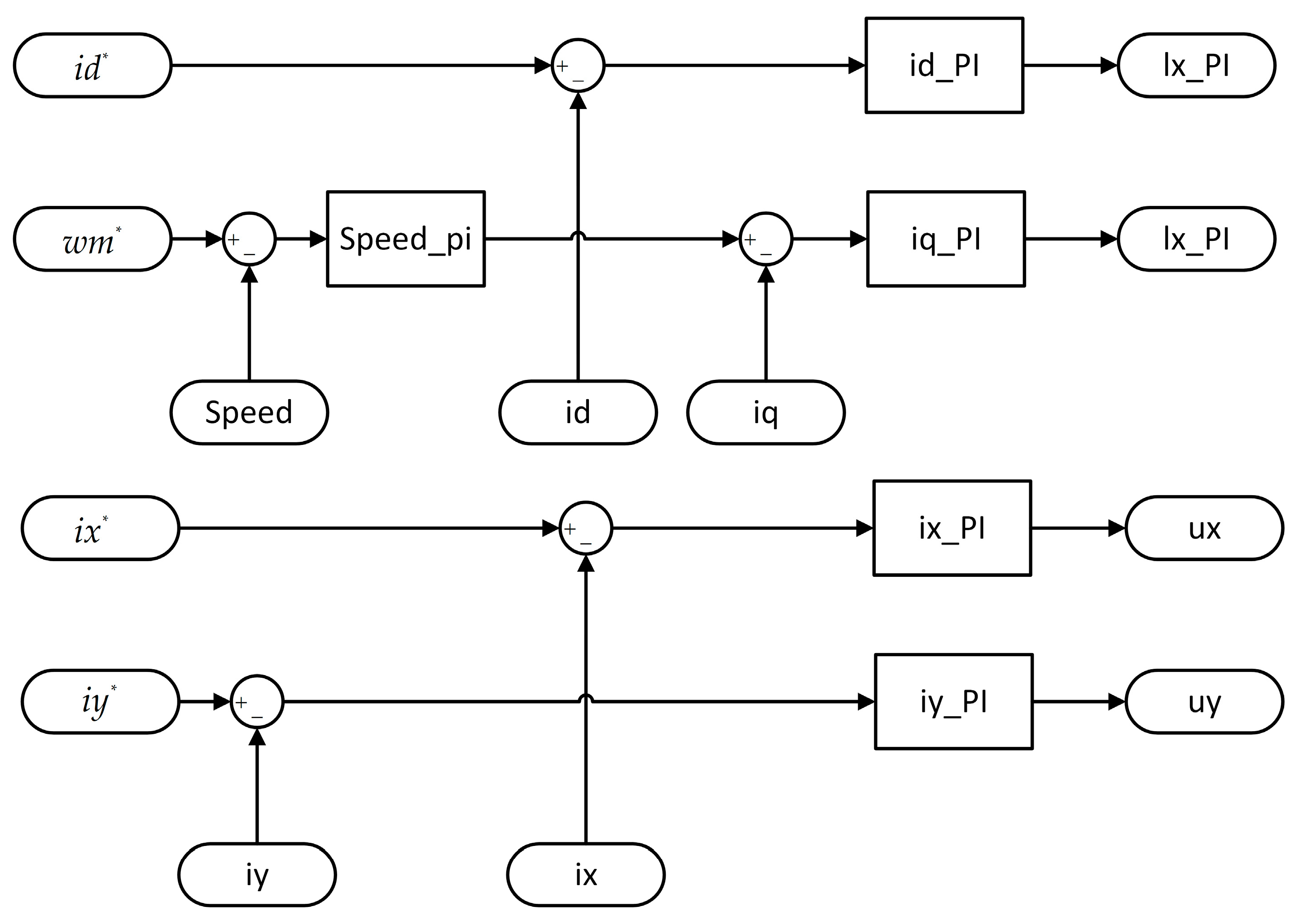
In Figure 8, speed_pi represents the PI regulator for the speed loop, while ld, lq, lx, and ly denote the PI regulators for the D-axis, Q-axis, X-axis, and Y-axis of the dual three-phase permanent magnet synchronous motor. The target values for these regulators are represented by ld*, wm*, lx*, and ly*, with ud, uq, ux, and uy indicating the output values.
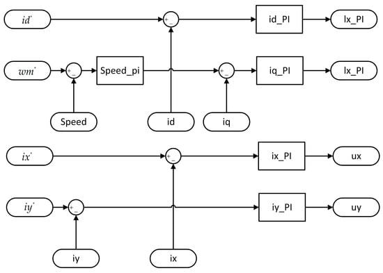
Figure 8.
P model of the regulators for speed and current loops. speed_pi: PI regulator for the speed loop. ld, la, lx, and ly: PI regulators for D-axis, Q-axis, X-axis, and Y-axis of dual three-phase permanent magnet synchronous motor. ld*, wm*, lx*, and ly*: Target values for regulators. ud, uq, ux, and uy: Output values.
3.3. Torque-Balancing Output Method for Dual Three-Phase Motors
The VSD coordinate transformation approach is employed to map the variables of a dual three-phase permanent magnet synchronous motor onto three distinct, mutually orthogonal subspaces: the subspace, the subspace (harmonic components), and the zero-sequence subspace. For analytical simplicity, a dual three-phase permanent magnet synchronous motor is modeled as an ideal motor under the following assumptions: (1) Stator currents and air-gap flux produced by the rotor’s permanent magnets are sinusoidally distributed; (2) Mutual inductance coefficients associated with leakage flux are neglected; (3) Eddy current losses are disregarded; (4) Hysteresis losses of the permanent magnets are omitted; (5) Magnetic saturation effect in the rotor core is ignored; (6) No damping windings are installed on the motor rotor.
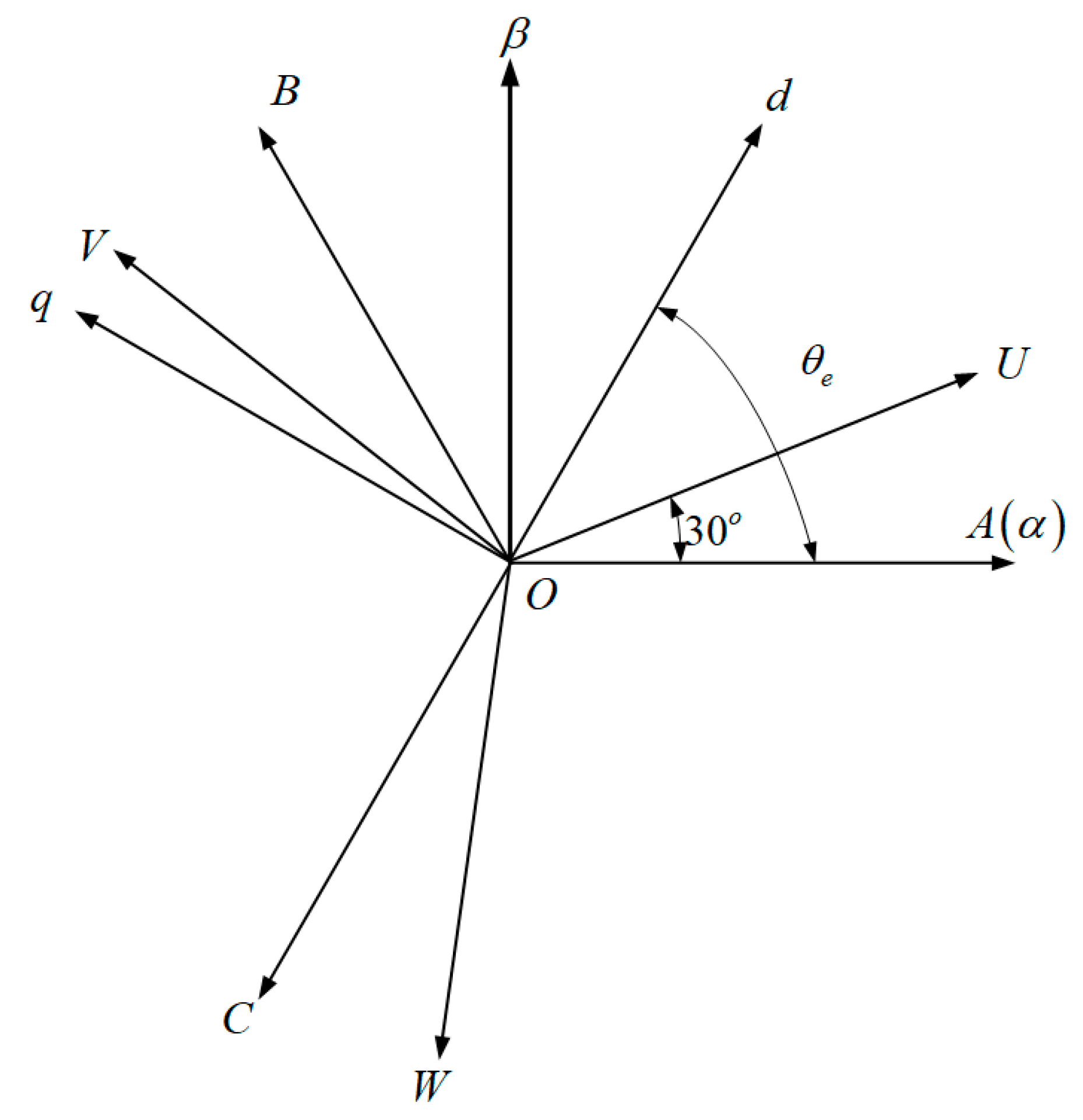
In Figure 9, transformation of the dual three-phase motors variables from natural ABC and UVW coordinate systems to a stationary coordinate system under the axis introduces harmonic and zero-sequence components.
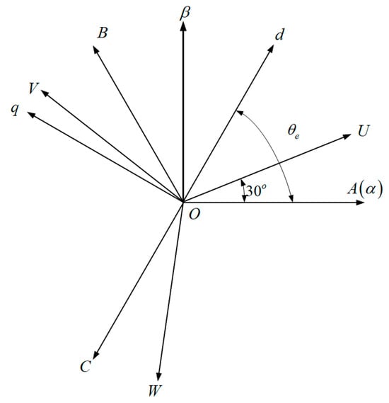
Figure 9.
VSD coordinate system for dual three-phase permanent magnet synchronous motor.
The stationary coordinate system under the axis is then transformed to achieve a synchronous rotating coordinate system under the axis.
Based on Equations (15) and (16), the following is derived:
Equation (17) is utilized to decouple torque components of the two winding sets of the dual three-phase permanent magnet synchronous motor, introducing the subspace (harmonic components) to enhance motor performance. Input quantities for vector control of the dual three-phase permanent magnet synchronous motor are calculated using the speed loop and current loop regulators P, as detailed in Section 3.2.
Contrasting with traditional permanent magnet synchronous motor drive systems, the dual three-phase permanent magnet synchronous motor drive system offers a larger array of voltage vectors and higher modulation complexity. Integrating spatial distribution of the six-phase drive bridge arms of the dual three-phase permanent magnet synchronous motor with the coordinate transformation matrix from Equation (17), the spatial voltage vectors generated by the two-level six-phase inverter in the and planes are represented as follows:
In Equation (18), to denote specific switch states of phases A through F of the six-phase inverter, designed to approximate an output voltage waveform to an ideal sinusoid, where 1 indicates the upper bridge arm conducting at a high level, and 0 signifies the lower bridge arm conducting at a low level.
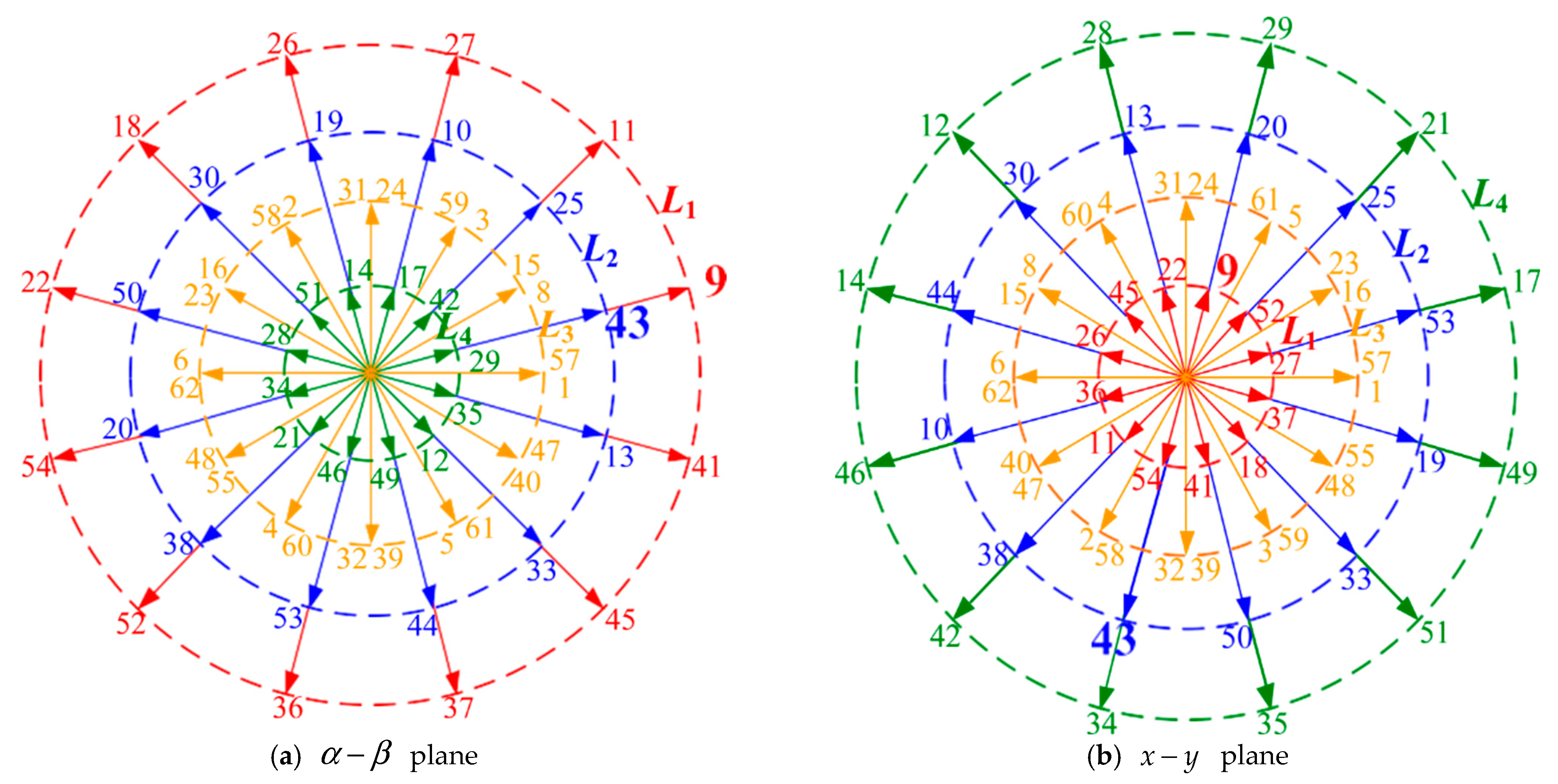
The six-phase two-level voltage source inverter can produce a total of 64 (26) switch states. These 64 vectors, as illustrated in Figure 10 and according to Equation (18), are mapped onto the and planes. The voltage space–vector numbers in the figure correspond to decimal equivalents of the binary switch state . For example, vector 9 corresponds to the switch state 001001 for . In Figure 10, voltage space vectors are categorized into , , , and , and these four groups are color coded based on their magnitudes with red, blue, orange, and green, respectively. Amplitudes of the vectors in each group are presented in Table 1.
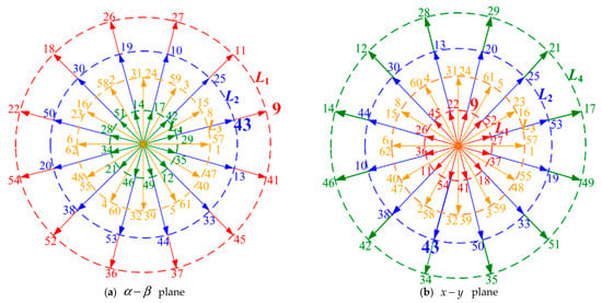
Figure 10.
Voltage space–vector diagrams of the six-phase two-level inverter. L1 (red), L2 (blue), L3 (orange), and L4 (green) are voltage space vectors.

Table 1.
Amplitudes of six-phase two-level voltage space vectors.
Observations from Figure 10 and Table 1 reveal correlations in mapping of the voltage space vectors across the and planes. Initially, vectors from Group L1 occupy the outermost layer of the plane; however, they are positioned at the innermost layer on the plane. Additionally, vectors with identical directions within Group L1 and Group L2 on the plane exhibit inverse directions on the plane. For instance, Vector 9 of Group L1 and Vector 43 of Group L2 share the same direction on the plane but display opposite directions on the plane. Given that substantial harmonic currents on the plane of dual three-phase motors are predominantly triggered by non-zero voltages on the plane, harmonization of these harmonic currents can be effectively managed by ensuring the composite voltage vector on the plane is nullified. Previous studies have adopted the constraint of zero synthesized voltage on the plane, utilizing four proximate original-voltage vectors to directly synthesize a reference voltage on the plane. However, these modulation strategies typically involve complex matrix transformations and vector synthesis processes. To simplify the vector synthesis process, this paper proposes a two-step vector synthesis approach for the two-level dual three-phase drive system, based on characteristics of the original voltage vectors on the and planes. Initially, the method utilizes a condition of zero volt-second equivalent voltage on the plane as a constraint, synthesizing harmonic-free vectors from the two original voltage vectors, followed by synthesis of a reference voltage vector from the two newly synthesized vectors.
In the first step of the two-step vector synthesis method, to maximize utilization rate of the bus voltage, vectors from Groups L1 and L2 with the same direction on the plane are selected to synthesize a harmonic-free vector. With the constraint of zero volt-second equivalent voltage on the plane, 12 non-zero harmonic-free vectors are synthesized on the plane, as shown in Figure 11. These 12 harmonic-free vectors divide the plane into 12 sectors, S1–S12. For example, Vector 9 of Group L1 and Vector 43 of Group L2 combine to form a harmonic-free vector V1. According to Table 1, during synthesis of a harmonic-free vector, the duty-cycle ratio coefficients PL1 and PL2 for the vectors from Groups L1 and L2 have specific constraint relationships:
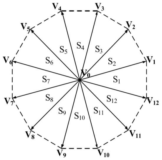
Figure 11.
Harmonic-free vectors in the plane. V1 through V12, which divide the plane into sectors S1–S12, are synthesized from vectors in Groups L1 and L2 that are oriented in the same direction on the plane.
Based on these constraint relationships, the duty-cycle ratio coefficients and can be resolved as and , respectively. Amplitude of the harmonic-free vector can be expressed as:
Using the amplitude of the harmonic-free vector from Equation (20), DC bus voltage-utilization rate for the proposed two-step vector synthesis method is calculated to be 0.577.
In the second step of the two-step vector synthesis method, the 12 newly synthesized harmonic-free vectors are used to synthesize a reference voltage vector on the plane. Figure 12 uses Sector S1 as an example to illustrate the basic principle of synthesizing a reference voltage vector Vref. It is evident that the method for synthesizing the reference voltage vector in this step aligns with the vector synthesis principles of three-phase motor drive systems. According to the volt-second balance principle, action time ratios TV1 and TV12 for the harmonic-free vectors V1 and V12, used to synthesize the reference voltage vector Vref in Sector S1, can be determined.
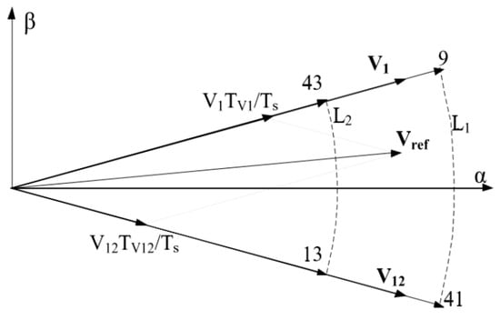
Figure 12.
Synthesis principle of reference voltage vectors for Sector S1 from Figure 11. V1 and V12 are harmonic-free vectors defining Sector S1 on the plane. TV1 and TV12 are action time ratios for V1 and V12, respectively. Vref is the reference voltage vector for Sector S1.
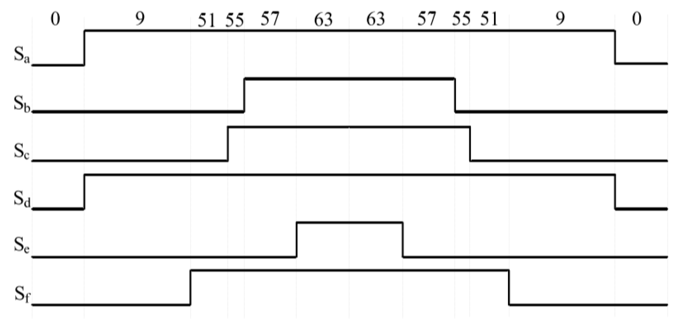
In the two-step vector synthesis method, reference voltage vector synthesis requires participation of four original vectors. To reduce unnecessary switching actions, this paper, based on the volt-second balance principle, centers high-level states of each phase as shown in Figure 13.

Figure 13.
Switching sequence of the six-phase two-level inverter in Sector S1.
In Equation (18), : Comparison of six-phase inverter on-time.
The aforementioned method enables the dual-redundancy SBW system to evenly distribute torque output in redundancy control mode, thereby enhancing the system’s safety and reliability.
3.4. Degraded System Fault-Tolerant Control for Dual Three-Phase Motors
Since the dual-redundancy SBW system is designed with redundancy theory, it is equipped with fault-tolerance capabilities. This allows the steering system to continue operating even when a fault occurs, necessitating monitoring of the system’s operational status. When a fault affects one set of windings or its associated circuit within the dual three-phase motors, the system can degrade the faulty winding and perform fault-tolerant processing. The steering system continues to control the normal winding, which continues outputting torque and completing steering functions, as depicted in Figure 14.
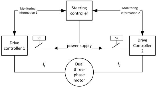
Figure 14.
System monitoring and degraded fault-tolerant control structure. S1 and S2 represent disconnection signals to their associated drive controllers.
In Figure 14, the steering controller provides real-time monitoring of drive controllers 1 and 2, monitoring the windings of the dual three-phase motors and exchanging status information. In this structure, any fault in the drive controllers or their circuitry can be detected by the steering controller. Should the SBW execution system degrade, for example, should drive controller 1 or its associated control circuit fail, the steering controller can identify the fault, send a disconnection signal S1, and cease sending control signals to drive controller 1, achieving fault-tolerant processing for the SBW system.
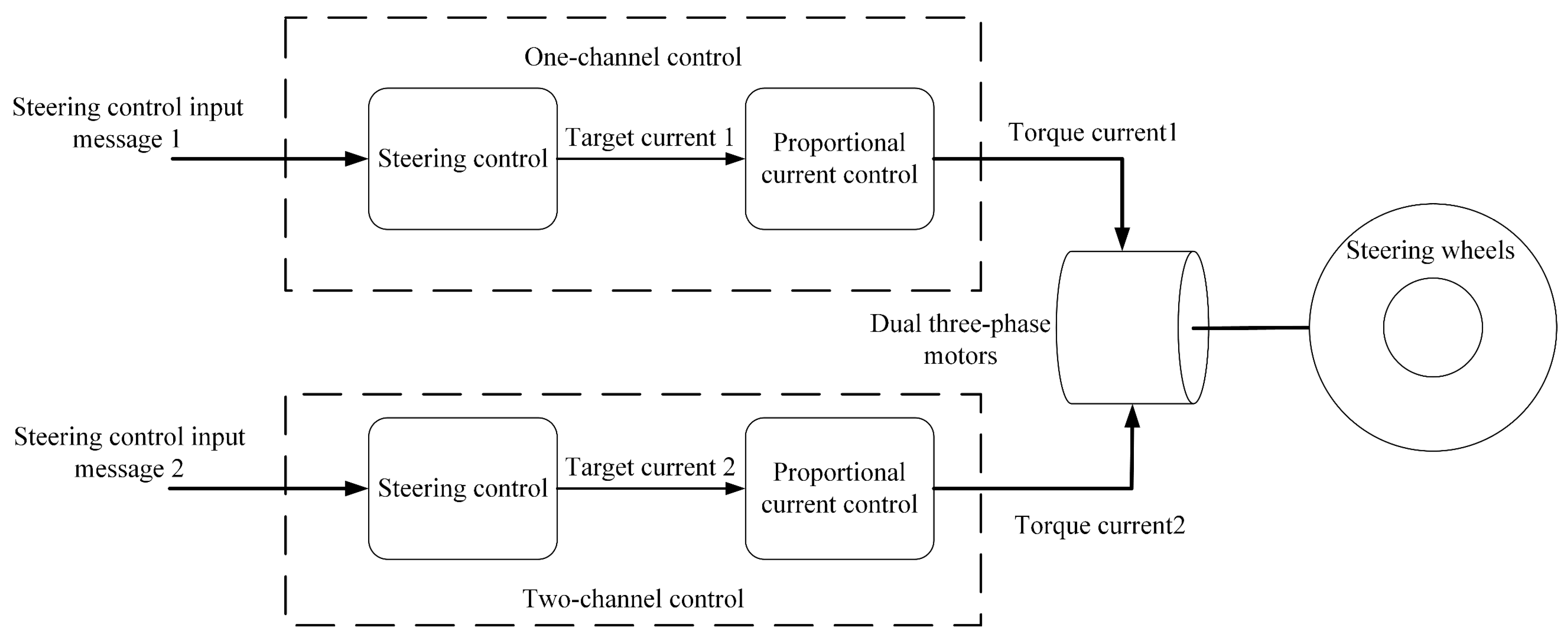
Figure 15 illustrates the system control architecture during normal operation of the SBW system, where both channels work in tandem to control coordinated operation of the dual three-phase motors, with the SBW system handling redundancy processing.
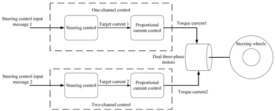
Figure 15.
Normal control architecture of the dual-redundancy system.
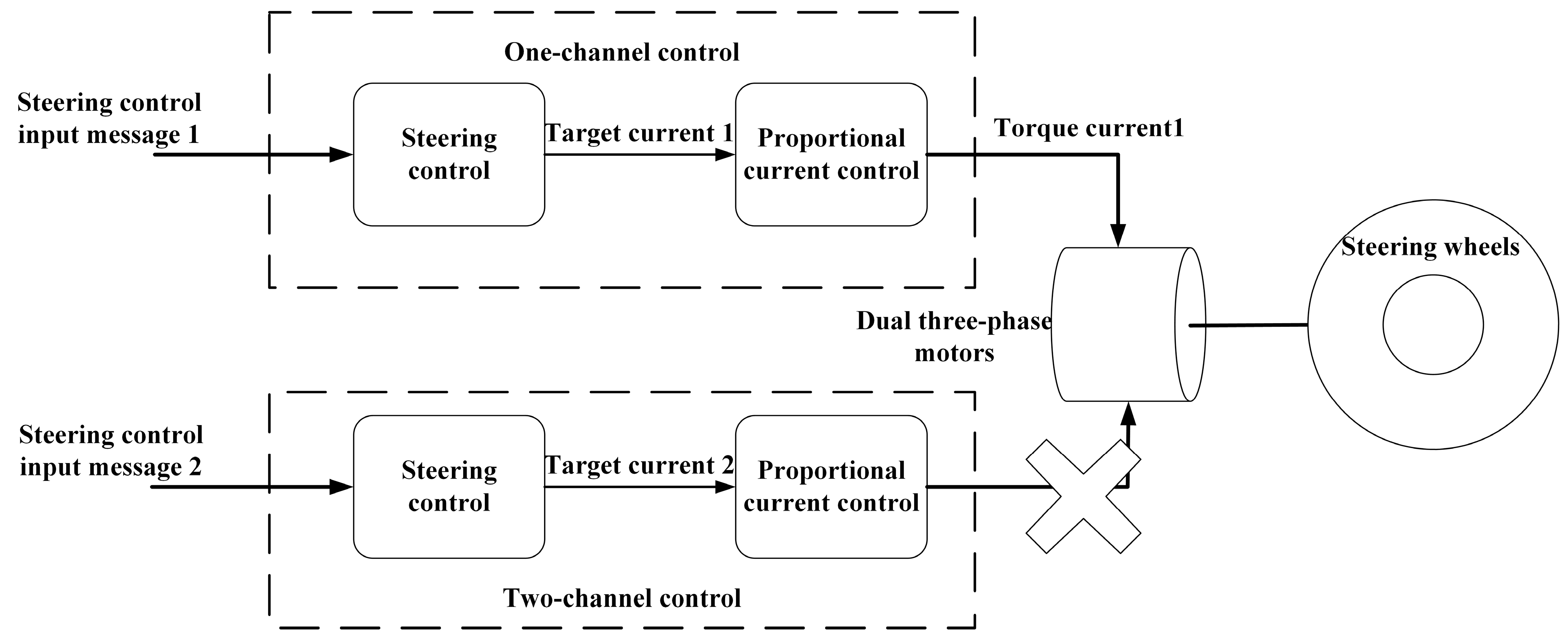
Figure 16 displays system control architecture following a fault in one channel of the redundant SBW system. Due to failure of channel 2, the SBW system is degraded, and as shown in Figure 14, the power supply to channel 2 is disconnected, leaving channel 1 operational.

Figure 16.
Degraded control architecture of the dual-redundancy system, showing disconnection of channel 2 from the dual three-phase motors.
During fault degradation and fault-tolerant processing of the SBW system, it is necessary to reorganize control of the dual three-phase motors in order to continue executing steering functions. The subsequent analysis examines the control processes of the dual three-phase motors before and after a fault in the dual-redundancy SBW system.
When the dual-redundancy SBW system is free of faults, the mechanical system’s dynamic model is as follows:
where and are torques of the two sets of windings of the dual three-phase permanent magnet synchronous motors, is rotational inertia of the dual three-phase motors, is angle of rotation of the dual three-phase motors, is signal function, is frictional resistance of the system, and is the return torque from the ground.
The torque characteristic equation for dual three-phase motors with two sets of windings is:
In Equations (22) and (23), is the torque coefficient of the steering motor and is mechanical efficiency. Since each dual three-phase motor’s sets of windings are the same, it can be assumed that motor parameters are the same for both sets of motor windings.
Given that the mechanical dynamic process is significantly slower than the current loop response of the dual three-phase motors, and to focus on the upper control process analysis, the current loop response is simplified to a proportional link.
For closed-loop position and closed-loop speed control of the two sets of windings, their output target currents are equal. After Laplace transformation, it is:
In Equation (26), is the closed-loop position output, is the velocity feedback, and is the closed-loop speed output.
To facilitate analysis of system characteristics during steering, Equation (21) simplifies the steering system’s dynamic equation. Since the steering system does not rotate during steady-state turns, the system friction is minimal and can be neglected. Thus, magnitude of self-aligning torque from the ground is related to the steering system’s angle and the vehicle speed. Assuming a direct proportionality between the ground self-aligning torque and the steering wheel angle, taking the Laplace transform of the simplified steering system dynamic equation yields:
In Equation (27), is the coefficient of proportionality between the ground return moment and the steering wheel angle.
From Equations (22)–(27), the system’s transfer function is derived:
It is evident from Equation (29) that after the system stabilizes, it can achieve indistinguishable following. All parameters in the transfer function are positive, and according to the Routh criterion, the condition for system stability is:
Substituting Equations (28)–(32) into Equation (33) results in:
As per Equation (34), the prerequisite for the steering system’s stability is that parameters of the position controller and the speed loop meet the aforementioned conditions. When a fault occurs in one winding of the dual three-phase motors in the SBW execution system, and only one set of windings operates normally, the original system balance is disrupted. With only one set of windings controlling, the system requires degradation and reorganization. The system’s transfer function is reorganized as:
From Equations (35)–(40), it is known that when , the SBW system, after degradation and reorganization, still maintains indistinguishable steady-state following. According to the Routh criterion, the condition for the system to remain stable is:
During a switch to fault-tolerant control of degraded dual three-phase motors in the dual-redundancy SBW system, an angular deviation occurs due to disruption of the mechanical force balance of the steering system. Frictional resistance from the road and mechanical structure that opposes the steering direction can suppress the occurrence of steering system oscillations.
In the process of driving, a fault-tolerant steering system, especially for SBW systems, can ensure that after a series of degradation and fault-tolerant treatments, the vehicle maintains its steering execution ability, preventing traffic accidents and ensuring the safety of drivers and passengers.
3.5. Fault Diagnosis
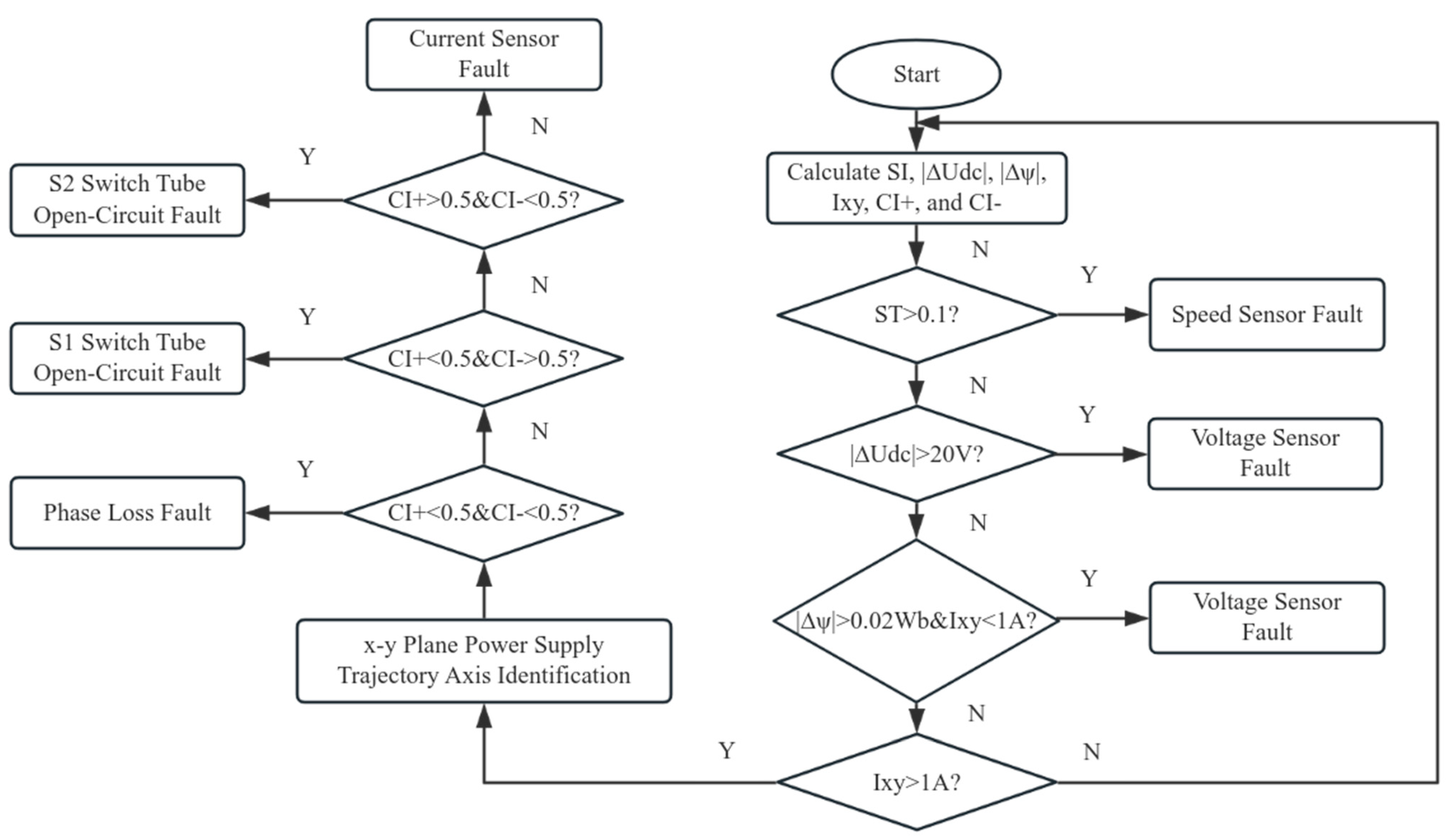
The dual three-phase permanent magnet synchronous motor drive system powered by a two-level inverter, as proposed in this paper, adopts a comprehensive diagnostic method for various fault types. This method primarily targets diagnoses of speed sensor faults, voltage sensor faults, current sensor faults, phase loss faults, and switch tube open-circuit faults. In this study, diagnosis of speed sensor faults is achieved by continuously monitoring the difference between measured and estimated rotational speeds. Given the high requirement for diagnosing rapid changes in DC bus voltage sensor errors, this type of fault diagnosis is realized by monitoring variation in the DC bus voltage-feedback value within a single sampling period. Diagnosis of gradual changes in DC bus voltage sensor errors is achieved by monitoring the difference between magnetic flux estimated by the current model-based flux observer and the voltage model-based flux observer. To simplify the diagnostic process, current sensor faults, phase loss faults, and switch tube open-circuit faults are diagnosed synchronously using the same method based on analyses of the x − y plane current trajectories. Figure 17 illustrates the comprehensive fault diagnosis flowchart, with diagnostic frequency being the same as the sampling frequency. The proposed comprehensive diagnostic method utilizes six indicative variables (SI, |∆Udc|, |∆ψ|, Ixy, CI+, and CI−) along with corresponding thresholds to comprehensively diagnose the five types of faults. In the diagnostic flowchart shown in Figure 18, the six indicative variables are first updated in real time according to sampling signals newly acquired from various sensors in the drive system during each sampling period. Considering coupling factors between different fault diagnoses and varying requirements for diagnostic speed, the diagnostic sequence is as follows: speed sensor fault diagnosis, sudden error in the DC bus voltage sensor fault diagnosis, gradual error in the DC bus voltage sensor fault diagnosis, and synchronous diagnosis of other faults.
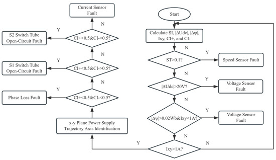
Figure 17.
Comprehensive fault diagnosis flowchart for multiple faults in two-level system. SI: Speed sensor fault indicator variable, fault threshold SI > 0.1. |∆Udc|: Sudden error voltage sensor fault indicator variable, fault threshold |∆Udc| > 20 V. |∆ψ|: Gradual error voltage sensor fault variable, fault threshold |∆ψ| > 0.02 Wb. Ixy: Amplitude of feedback current in the plane, fault threshold Ixy > 1 A. CI+ and CI− Switch tube open-circuit variables. Y: yes. N: no.
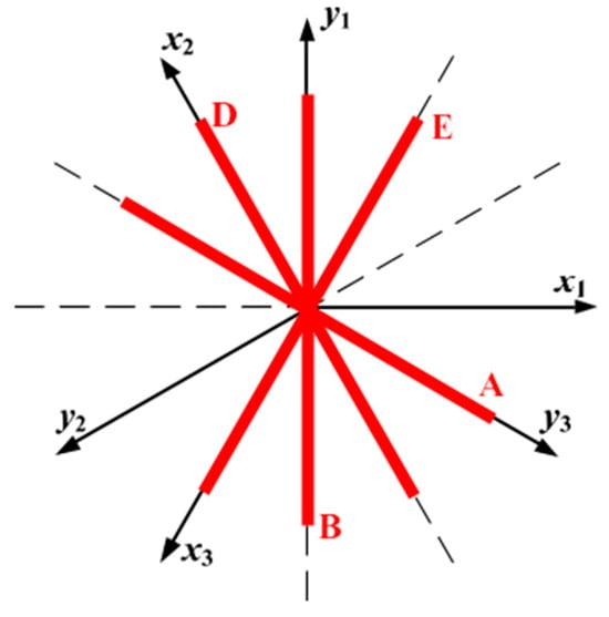
Figure 18.
Feedback current trajectories on the plane under various current sensor faults. Orthogonal coordinate systems , , and . A, B, D, and E represent current sensor faults in phases A, B, D, and E.
3.5.1. Speed Sensor Fault Diagnosis
The most common method for speed sensor fault diagnosis is to continuously monitor the difference between the measured and estimated rotational speeds [21,22]. To reduce complexity of the diagnosis, the estimated rotational speed in this paper is indirectly obtained by estimating rotational speed of the magnetic flux [23]. In this way, the estimated rotor angular velocity can be expressed as:
where is rotor position angle, is stator chain angle, is torque angle, is rotating speed of the stator chain, and is the differential value of the torque angle. Since is much smaller than in actual operation, an estimated rotor angular speed can be approximated as the stator chain rotation speed . When the speed sensor fails, the speed measured by the speed sensor will deviate from the actual speed, but the estimated speed in Equation (42) still reflects the actual speed of the motor relatively accurately. Therefore, the difference between the motor speed feedback value and the speed estimation value is close to 0 when the speed sensor is normal and deviates from 0 when the speed sensor is faulty. Based on this characteristic, the speed sensor fault indicator variable SI is defined as:
In Equation (43), represents rated speed of the motor, which is set at 1000 rpm for this study. To ensure swift diagnosis of speed sensor faults and to prevent misdiagnosis, and after considering actual measurements and incorporating a certain margin, the threshold for the speed sensor fault indicative variable is set to 0.1. A value of indicates a fault in the speed sensor. Although coupling factors between different diagnostic methods may cause a slight increase in the speed sensor fault indicative variable SI when other faults occur, this minor increase is acceptable compared to the set threshold of 0.1. Therefore, the proposed method for diagnosing speed sensor faults effectively avoids misdiagnoses.
3.5.2. DC Bus Voltage Sensor Detection
Considering the timeliness of diagnosis, fault diagnosis of the DC bus voltage sensor is divided into two categories: sudden error fault diagnosis and gradual error fault diagnosis. Sudden error faults in voltage sensors can lead to rapid collapse of the motor drive system, necessitating faster diagnostic speed. In contrast, gradual error faults in voltage sensors have a less significant impact on the drive system, allowing for a more relaxed diagnostic speed requirement. Following the diagnosis of speed sensor faults, sudden and gradual error faults in the voltage sensor are diagnosed sequentially, as shown in Figure 18.
For a sudden error fault in the voltage sensor, this paper achieves fault diagnosis by continuously monitoring for sudden change in the DC bus voltage-feedback value. Based on characteristics of a sudden voltage jump in the voltage sensor, this paper defines the sudden error fault indicative variable of the DC bus voltage sensor as:
In Equation (44), is the DC bus voltage-feedback value in the current sampling period, and is the DC bus voltage-feedback value in the previous sampling period. Since the fault indicative variable is only related to the feedback value of the voltage sensor, it is not affected by any other faults. During normal dynamic operation, the DC bus voltage-feedback value will slightly fluctuate due to charging and discharging of the capacitor, but there will be no voltage jump. To ensure rapid diagnosis of a sudden error fault in the DC bus voltage sensor while avoiding false diagnoses, and after considering the change in the DC bus voltage during a single sampling period and leaving a certain margin, the threshold for the fault indicative variable is set to 20 V. When the fault indicative variable is greater than 20 V, a sudden error fault in the voltage sensor will be diagnosed before the voltage feedback value is introduced into the control system. Rapid diagnosis of the sudden error fault in the voltage sensor, combined with fault-tolerant control, can effectively prevent collapse of the drive system. Since this diagnostic method is specifically designed for voltage sensor sudden error faults with large changes in feedback voltage between adjacent two sampling periods, it is not suitable for diagnosing voltage sensor gradual error faults with small changes in feedback voltage between adjacent two sampling periods.
For voltage sensor error asymptotic faults, this paper realizes fault diagnosis by real-time monitoring of the difference between the output magnetic chain of the current model-based magnetic chain observer and the output magnetic chain of the voltage model-based magnetic chain observer . Voltage and magnetic chain equations of the dual three-phase permanent magnet synchronous motors are expressed as:
In Equations (45) and (46), , , and denote motor stator voltage vector, stator current vector, and stator chain vector, respectively. is the stator resistance, is the stator inductance matrix, is the permanent magnet chain amplitude, and is the rotor electrical angle.
The stator magnetic flux observer based on the voltage model, derived from Equation (45), can be expressed as:
The magnetic flux equation in the rotating coordinate system of the dual three-phase motors is:
The stator magnetic flux observer based on the current model, derived from Equation (49), can be expressed as:
This diagnostic principle relies on the fact that the magnetic flux observer based on the voltage model strictly depends on the DC bus voltage-feedback value when estimating stator magnetic flux, whereas the magnetic flux observer based on the current model does not require the DC bus voltage information. Under normal operation, both magnetic flux observers can accurately observe the stator magnetic flux. When a gradual error fault occurs in the DC bus voltage sensor, the stator magnetic flux estimated by the voltage model-based magnetic flux observer becomes erroneous, while the stator magnetic flux estimated by the current model-based magnetic flux observer continues to accurately reflect real-time stator magnetic flux. If the DC bus voltage-feedback sensor value is lower than the actual stator magnetic flux value, the stator magnetic flux estimated by the voltage model-based magnetic flux observer will also be lower than the actual stator magnetic flux, and vice versa. Consequently, a gradual error fault in the DC bus voltage sensor leads to a discrepancy in the stator magnetic flux estimate outputs from the two magnetic flux observers.
Based on the distinct responses of the two types of magnetic flux observers to a gradual error fault in the voltage sensor, this paper defines the gradual error fault indicative variable for the DC bus voltage sensor as:
To ensure rapid diagnosis of a gradual error fault in the DC bus voltage sensor and to prevent misdiagnosis, and after considering impacts of DC bus voltage fluctuations on the magnetic flux observations during dynamic operation and allowing for a certain margin, the threshold for the fault indicative variable is set to 0.02 Wb. When the fault indicative variable exceeds 0.02 Wb, and the current in the plane does not surpass the threshold, a gradual error fault has occurred in the DC bus voltage sensor, as depicted in Figure 18. Consideration of the current in the plane is to avoid misdiagnosing other faults as voltage sensor faults. In reality, due to coupling factors in fault diagnosis, current sensor faults, phase loss faults, and switch tube open-circuit faults can all result in incorrect magnetic flux calculations. These three types of faults can cause abnormal feedback current in the plane, whereas the feedback current in the plane will remain close to zero with voltage sensor faults. Therefore, real-time monitoring of the current in the plane during diagnosis of gradual error faults in the voltage sensor can prevent false diagnoses. It should be noted that a magnetic flux observer based on a current model requires rotor position angle to obtain the current in a synchronous rotating coordinate system, and a fault in the speed sensor can also lead to incorrect magnetic flux calculations. However, since diagnosis of speed sensor faults is faster than diagnosis of gradual error faults in the voltage sensor, speed sensor faults will not be misdiagnosed as voltage sensor faults.
3.5.3. Synchronous Diagnosis of Other Faults
Current sensor faults, phase loss faults, and open-circuit faults in switch tubes all lead to changes in the linear characteristics in the plane current trajectories. At the same time, there are differences in slope and symmetry of the plane current trajectories under these three types of faults. Commonality in the plane current trajectories under these conditions serves as the premise for synchronous diagnosis, while differences in the current trajectories create opportunities for identifying specific faults. To optimize the diagnostic process, this paper proposes a three-step diagnostic method based on analysis of the plane current trajectories for simultaneous diagnosis of these three types of faults, as shown in Figure 18.
The first step in comprehensive diagnosis is to monitor abnormal currents on the plane. Amplitude of the feedback current on the plane can be expressed as:
Under normal operating conditions, the amplitude of the plane current, , consistently remains near zero. Since current sensor faults, phase loss, and open-circuit faults in switch tubes all result in an abnormal increase in the current amplitude , this current amplitude can be utilized as an indicator for occurrence of any of these three types of faults. To ensure rapid fault diagnosis while avoiding false positives, threshold for the fault indication variable in this study is set at 1 A. If the fault indication variable exceeds 1 A, the drive system is experiencing a fault related to the current sensor, to phase loss, or to an open-circuit fault in a switch tube.
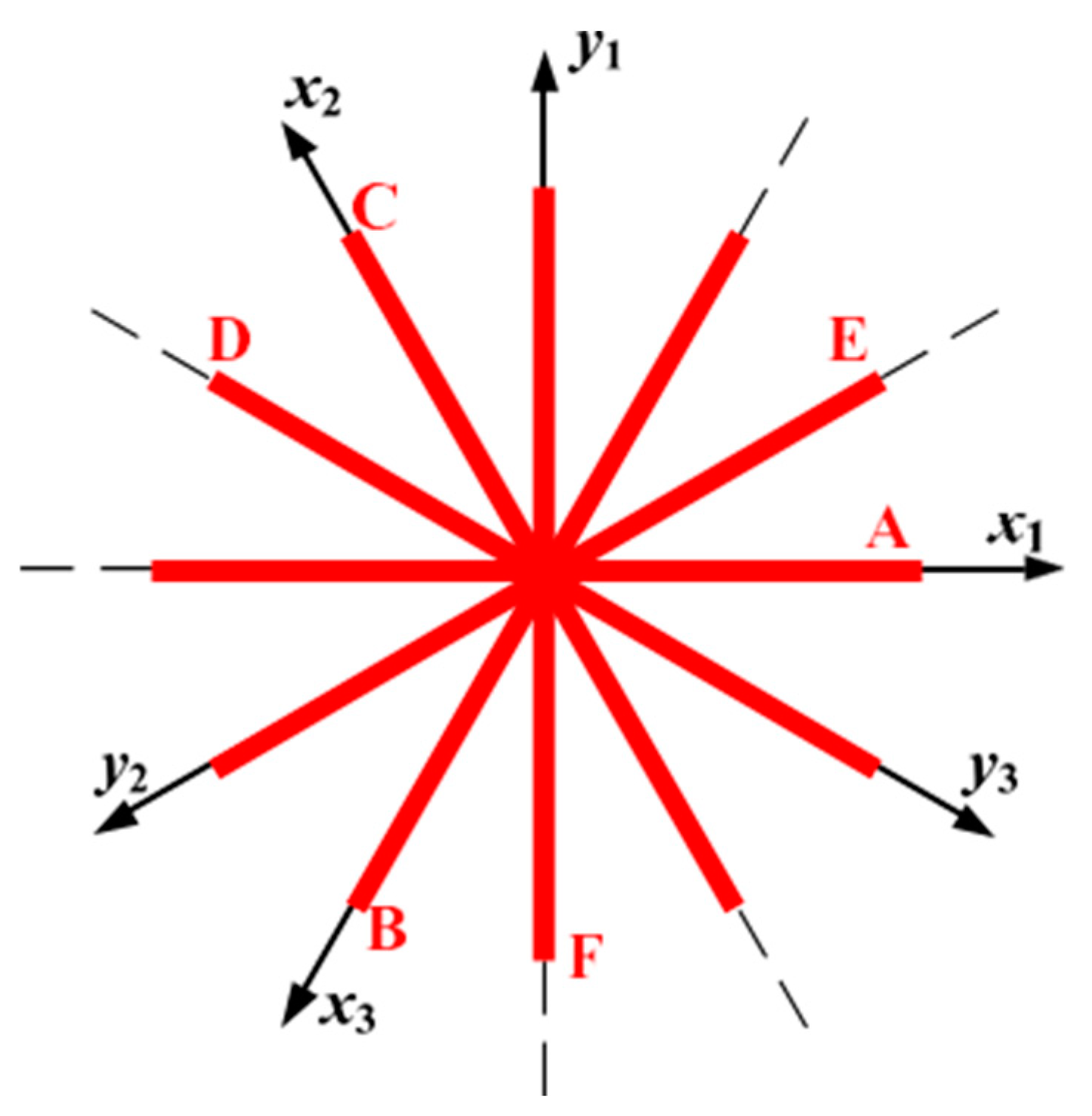
The second step in comprehensive diagnosis is to identify the axis on which the plane current trajectories reside during a fault. This is achieved by comparing the currents projected onto the coordinate axes of the plane. To facilitate fault analysis and diagnosis, three sets of orthogonal coordinate systems, each separated by 120°, have been established on the plane: , , and , as illustrated in Figure 19, Figure 20 and Figure 21. By coordinate transformation, the current components projected onto the six coordinate axes of the plane can be derived and expressed as:
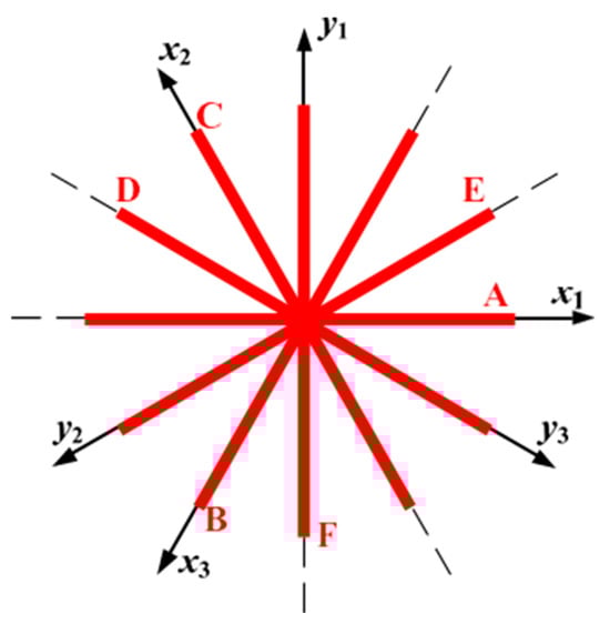
Figure 19.
Current trajectories on the plane under various phase-loss conditions. Orthogonal coordinate systems , , and . A–F represent phase loss faults in phases A–F.
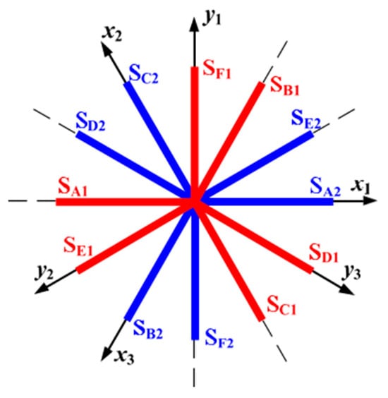
Figure 20.
Current trajectories on the plane under different switch tube open-circuit faults in a two-level inverter. Orthogonal coordinate systems , , and . − represent open circuit faults in phases A–F.
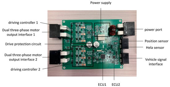
Figure 21.
Dual-redundancy SBW executive driver.
From analysis of current sensor faults, phase loss faults, and open-circuit faults in switch tubes, it is evident that all possible plane current trajectories under these conditions lie along one of the six coordinate axes. Consequently, the current component projected onto the coordinate axis perpendicular to the trajectory’s axis is approximately zero. Leveraging this trajectory characteristic, this study identifies the axis on which the plane current trajectory resides by obtaining and comparing average absolute values of the current components projected onto the six coordinate axes of the plane over one fundamental period following fault occurrence. Summarizing all the fault types presented in Figure 18, Figure 19 and Figure 20, each axis corresponds to three or four potential fault scenarios, as detailed in Table 2. For example, when the planar current trace is located in the axis, the system is experiencing one of four faults, namely, an open-circuit fault in phase D, an open-circuit fault in the switching tube at , an open-circuit fault in the switching tube at , or an open-circuit fault in the A-phase current sensor. Therefore, in the third step of the comprehensive diagnostics it is necessary to target a specific fault from the fault possibilities identified in the second step of the comprehensive diagnostics.
Table 2.
Fault possibilities corresponding to different coordinate axis directions.
The third step in comprehensive diagnosis is to pinpoint the type and location of the fault through phase current analysis. The synchronous diagnostic method proposed in this paper begins to calculate the average of positive half-cycle current absolute values and negative half-cycle current absolute values of the six-phase current over one fundamental period once the fault indication variable surpasses its threshold. These are denoted as , , , , , , , , , , , and . The average values of these twelve variables are represented as:
Ultimately, the ratio of these twelve variables to is utilized as a fault indication variable. Considering the plane current trajectory residing on the axis as an example, Table 2 indicates that the four fault possibilities corresponding to the axis are primarily centered on Phase D. Therefore, the specific fault can be identified by analyzing the current in Phase D. The fault indication variable for Phase D can be expressed as:
In conclusion, the multi-fault synchronous diagnostic method proposed in this paper, which includes monitoring the plane current, determining axis direction of the plane current trajectories, and locking down a specific fault, achieves synchronous diagnosis of current sensor faults, phase loss faults, and open-circuit faults in switch tubes.
4. Experimental Verification
To verify safety and reliability of the dual-redundancy SBW control system’s steering execution, initial comprehensive laboratory performance tests of the automotive steering gear were conducted to ascertain feasibility. Subsequently, a SBW test rig was assembled to simulate the dual-redundancy SBW system under real road conditions, performing redundancy control hardware-in-the-loop tests during dual-lane-change maneuvers and simulating motor winding circuit faults during steering execution processes to assess system degradation and fault-tolerance control. The constructed drive controller is depicted in Figure 17.
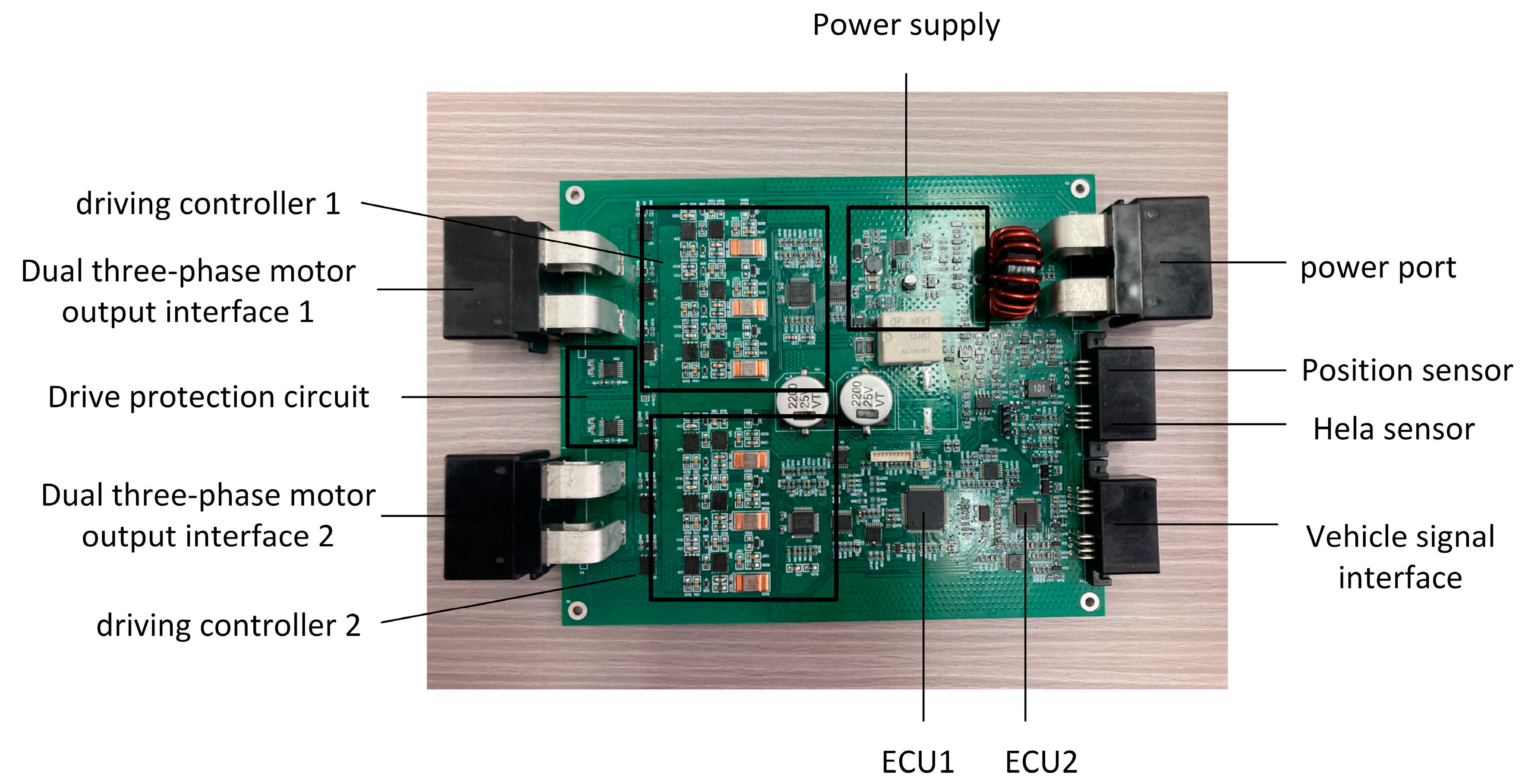
Figure 21 shows the SBW system driver, which incorporates two sets of motor drive circuits on a hardware redundancy basis to power the dual three-phase motors. Should one drive circuit fail, the other can continue to perform steering functions, ensuring the safety of drivers and passengers and meeting the safety and reliability requirements of SBW control.
4.1. Laboratory Comprehensive Performance Test of the Automotive Steering Gear
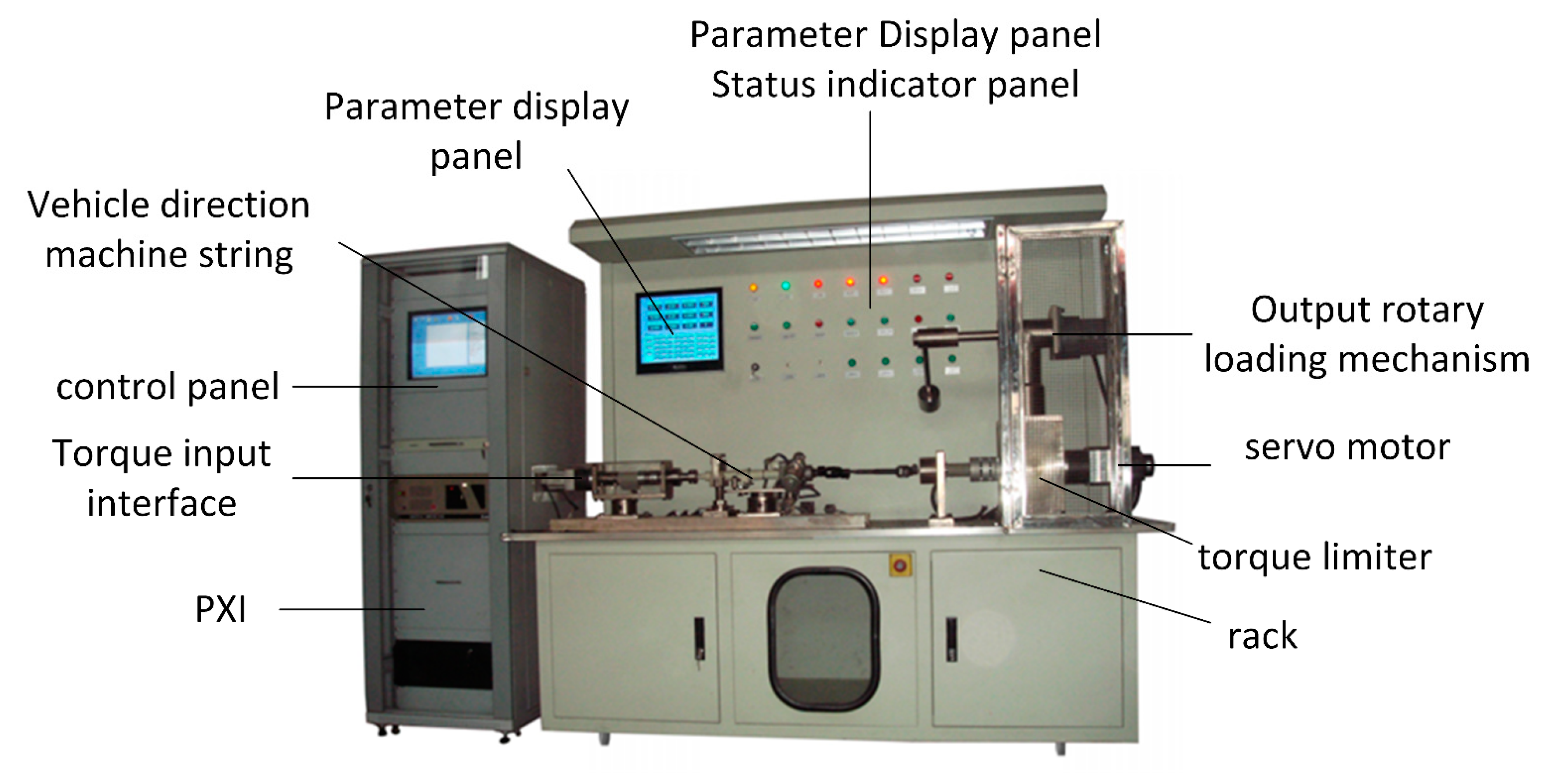
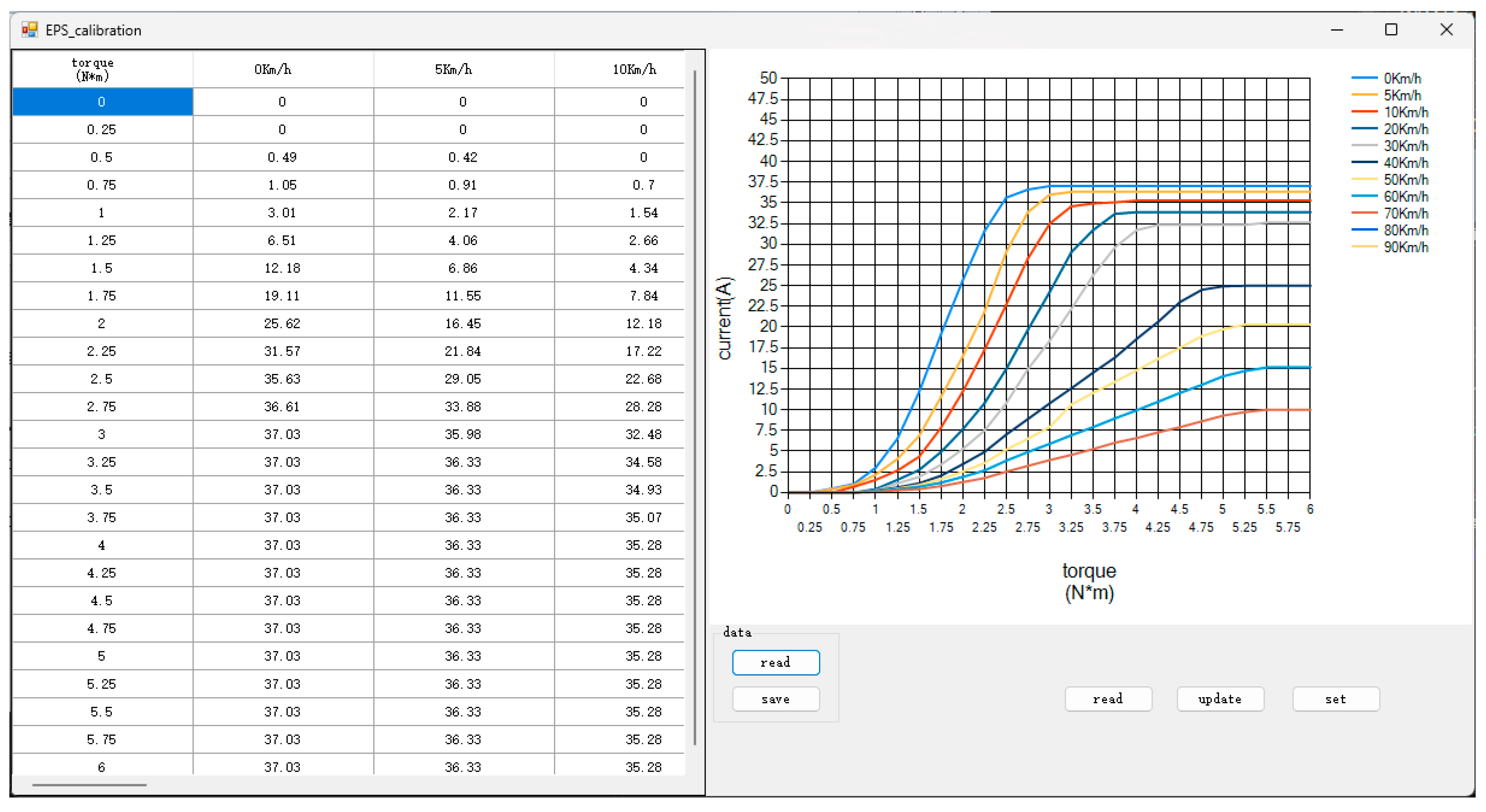
Utilizing the comprehensive automotive steering laboratory performance test rig in Figure 22, input torque/motor current characteristics tests were conducted on the dual-redundancy SBW system. Tests were performed at vehicle speeds of 0 Km, 5 Km/h, 10 Km/h, 20 Km/h, and 30 Km/h~90 Km/h, applying steering wheel torque inputs of 0 to 6 N*m to assess the current outputs of the dual three-phase steering actuator motor, thereby validating the SBW system’s redundancy function. The test results are presented in Figure 23.
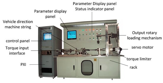
Figure 22.
Laboratory comprehensive performance test rig for automotive steering gear.
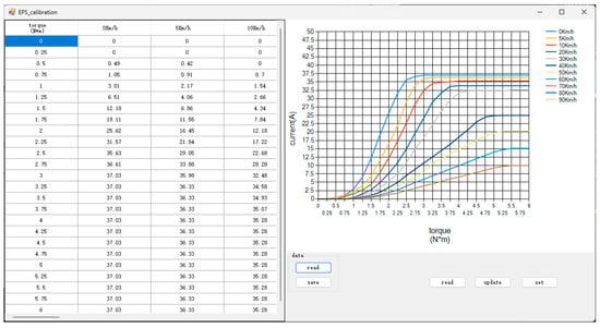
Figure 23.
Output torque–current curves of dual three-phase motors under various vehicle speeds and steering wheel torque inputs.
In Figure 23, the horizontal axis represents the torque input from the steering wheel, and the vertical axis represents the torque current output from the steering actuator motor. The test data indicate that the SBW system’s output torque followed the same curve as electric power steering assist, divided into a no-assistance zone, a main force zone, and an assistance saturation zone. The steering output torque was smooth and free from any abrupt torque changes, thereby confirming the effectiveness of the dual-redundancy SBW control system’s redundant function in terms of output torque.
4.2. Experimental Verification of Redundant Control of Steering System
The hardware-in-the-loop test of the dual-redundancy SBW system was carried out using the driving platform shown in Figure 24, simulating various conditions encountered by a vehicle during normal driving. The experimental parameters are shown in Table 3 and Table 4.
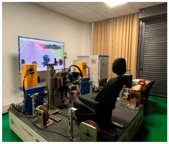
Figure 24.
Hardware-in-the-loop test rig.
Table 3.
Hardware-in-the-loop test parameters of the dual-redundancy SBW system.
Table 4.
Motor simulation parameters.
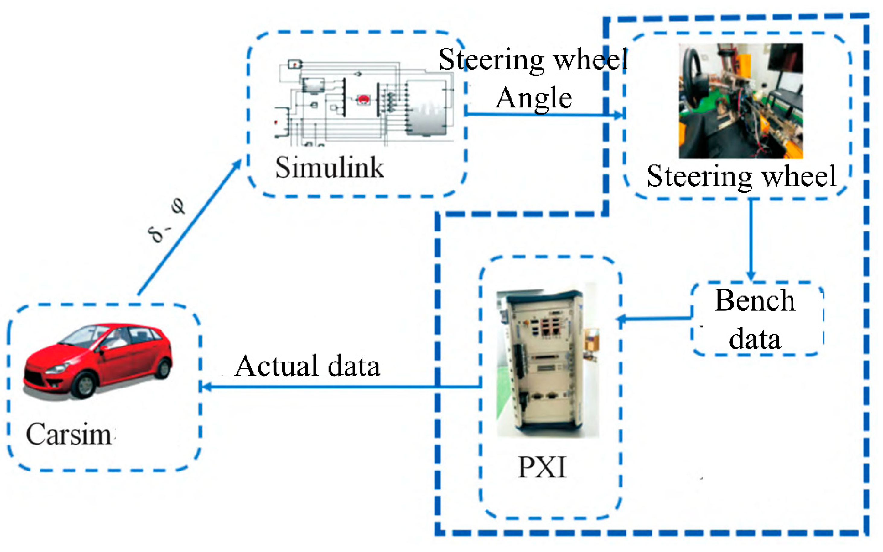
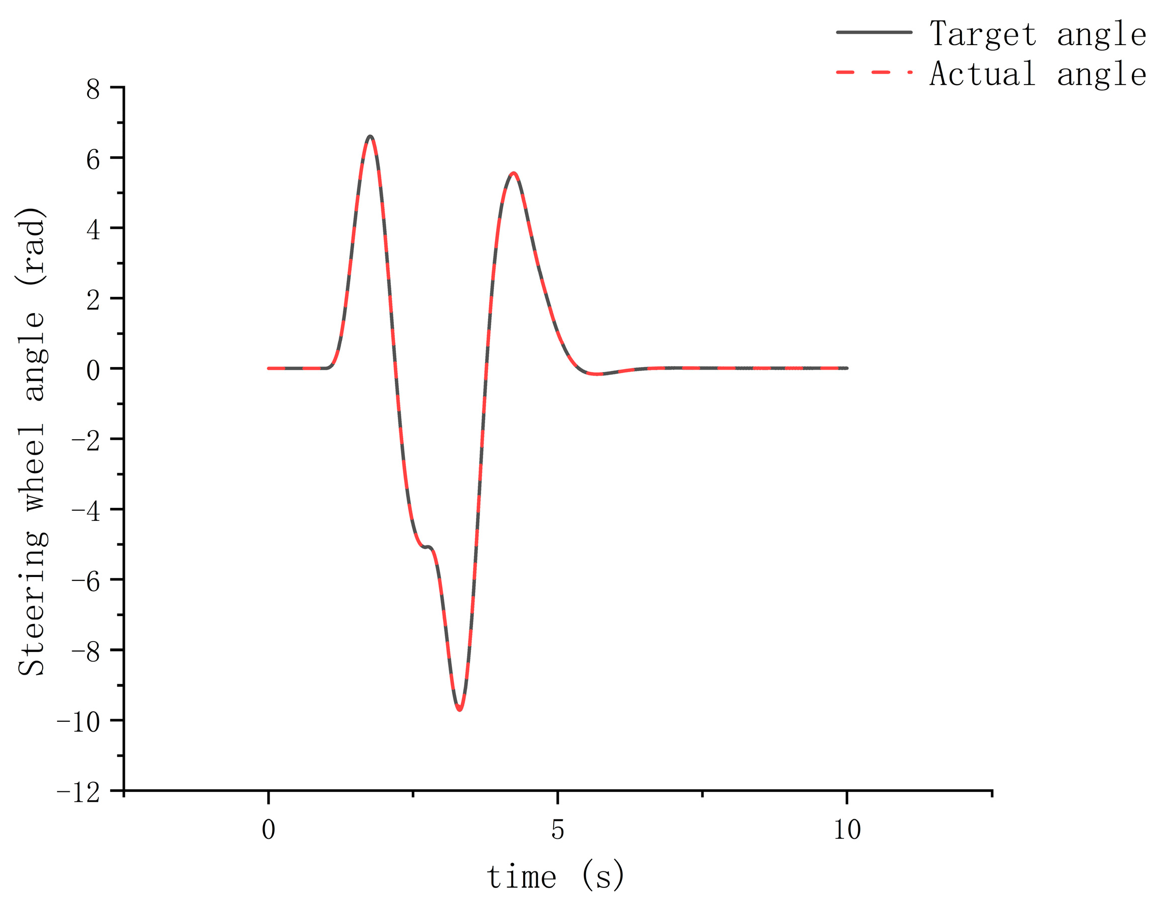
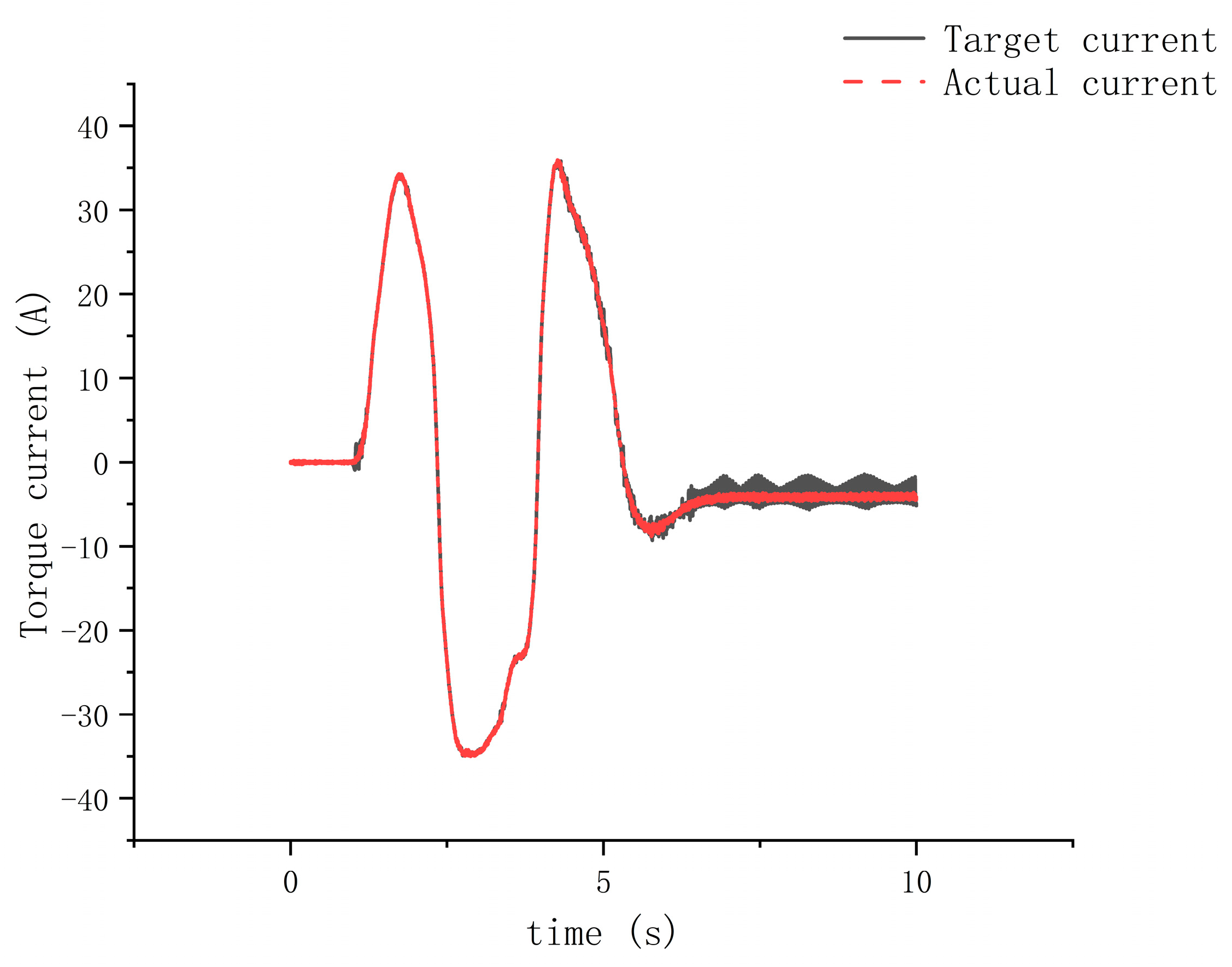
The experiment was conducted on the test rig according to the experimental principle shown in Figure 25, using a combined simulation with Simulink and Carsim. The vehicle was driven at a constant speed of 80 km/h, following the dual-lane-change trajectory depicted in Figure 26. The results are shown in Figure 27 and Figure 28, which display the vehicle’s steering wheel angle over time and the torque current output of the dual three-phase motors over time, respectively. Figure 27 indicates that the torque vector-space-decoupling control method for the dual three-phase motors balanced the output torque of the two winding sets, which were identical, resulting in equal torque outputs from both sets. When torque output of the dual three-phase motors’ winding sets becomes unbalanced to the point of being opposite, torque interference occurs. The torque vector-space-decoupling control method proposed in this paper spatially decouples the two winding sets to prevent occurrence of torque interference between dual winding sets. Additionally, the torque current output curve of the dual three-phase motors shown in Figure 28 fit well with the target current curve, and the curve was smooth, indicating that the dual-redundancy SBW system had good follow-up performance, and the redundancy function was executed without lag.

Figure 25.
Experimental principle of hardware-in-the-loop experiment using the test rig shown in Figure 24.
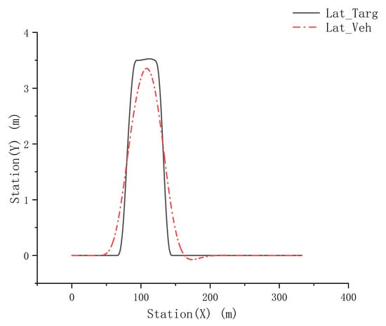
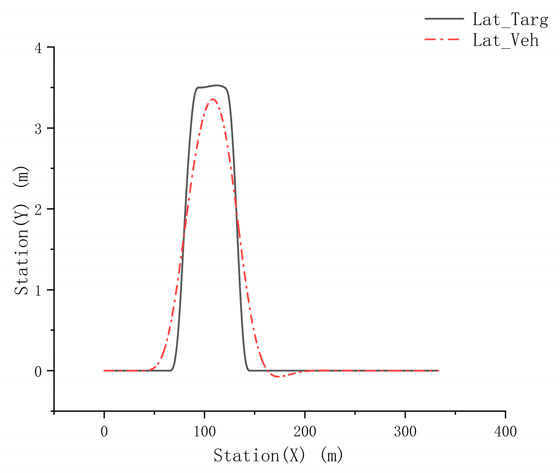
Figure 26.
Vehicle dual-lane-change trajectory during hardware-in-the-loop experiment using test rig shown in Figure 24.
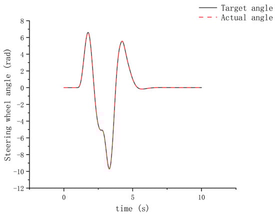
Figure 27.
Vehicle steering wheel angle during hardware-in-the-loop experiment using test rig shown in Figure 24.
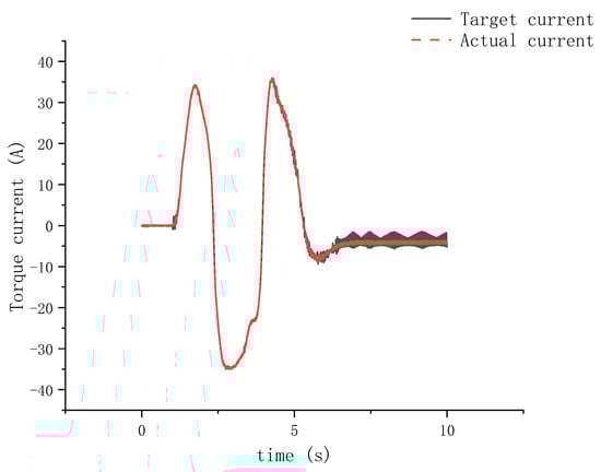
Figure 28.
Torque current output of dual three-phase motors during hardware-in-the-loop experiment using test rig shown in Figure 24.
Thus, the torque vector-space-decoupling control method for the dual three-phase motors is validated.
4.3. Experimental Verification of Fault-Tolerant Control of Steering System
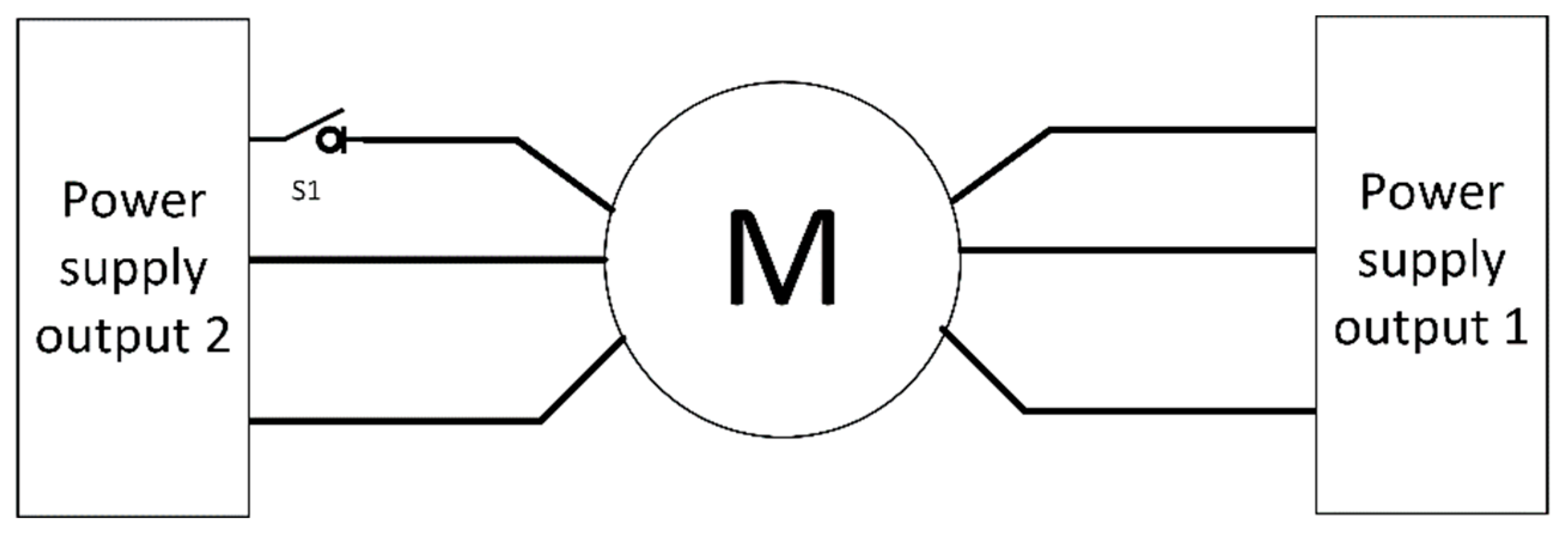
In the fault-tolerance experiment of the dual-redundancy SBW system, relays were installed on the power lines between the controller and the dual three-phase motors to simulate open-circuit faults in the motor windings, as shown in Figure 29. The steering wheel angle and torque current of the dual three-phase motors during the fault-tolerant control experiment are shown in Figure 30 and Figure 31, respectively.
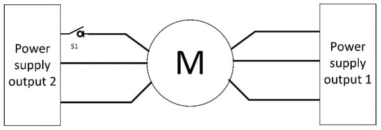
Figure 29.
Schematic diagram of motor open-circuit fault simulation. M is the controller.
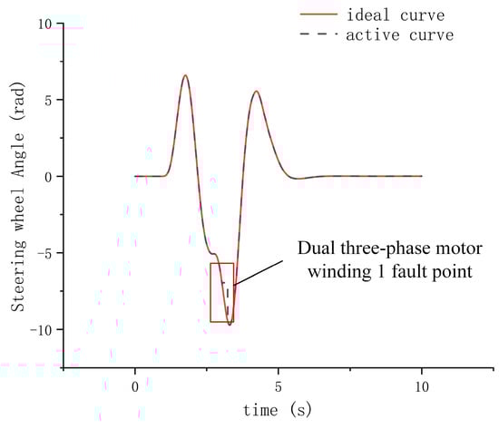
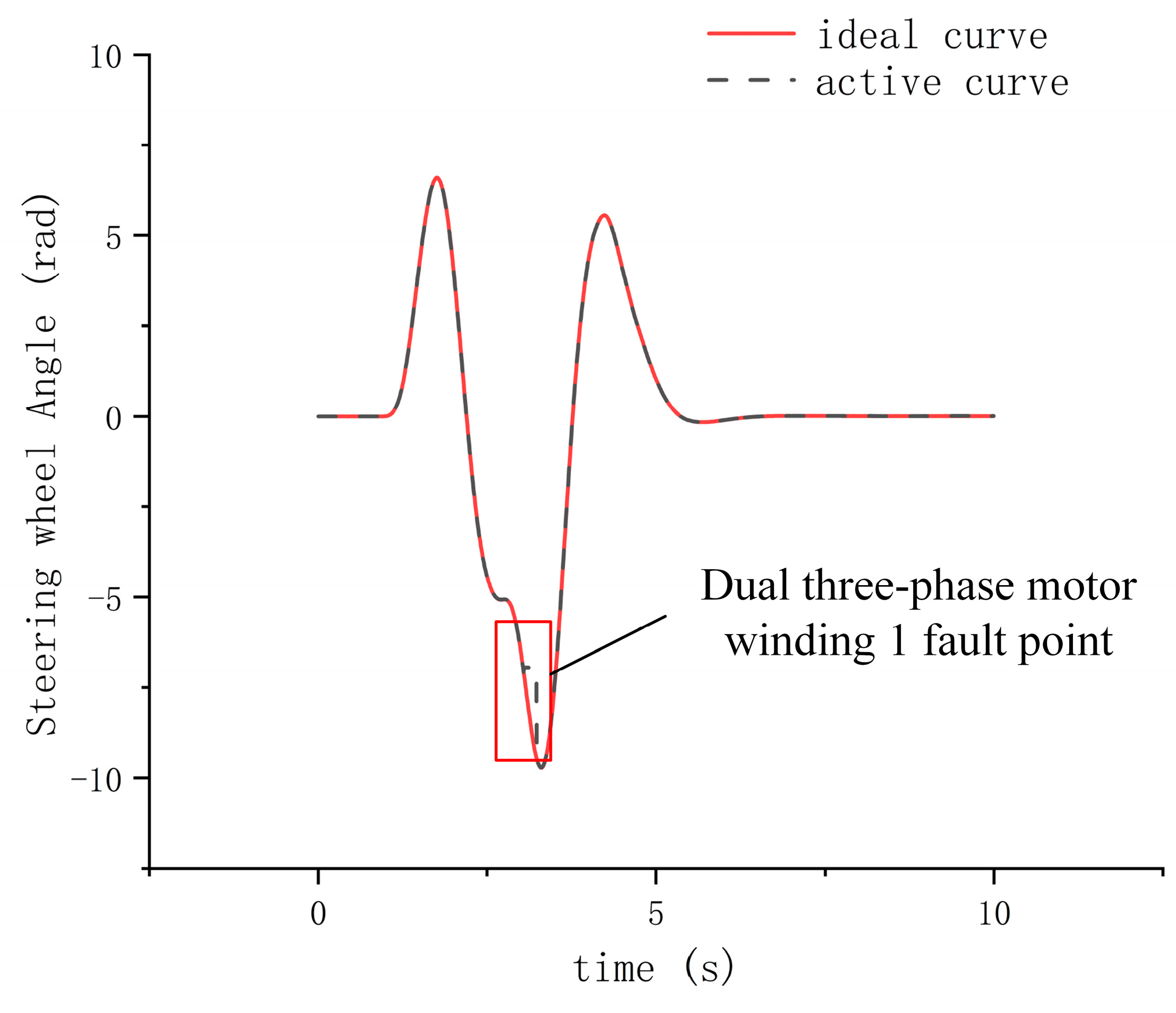
Figure 30.
Steering wheel angle under fault-tolerant control during fault-tolerance experiment.
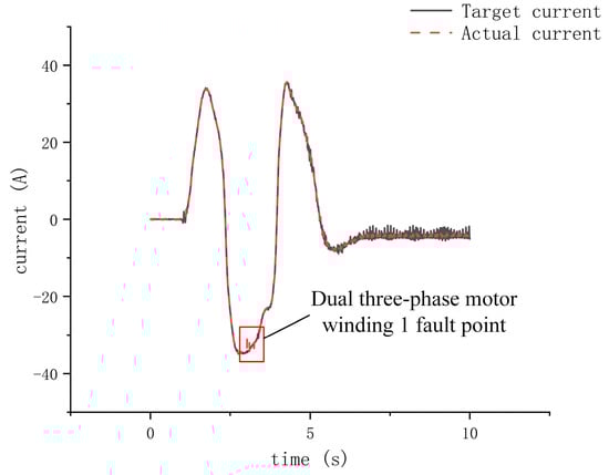
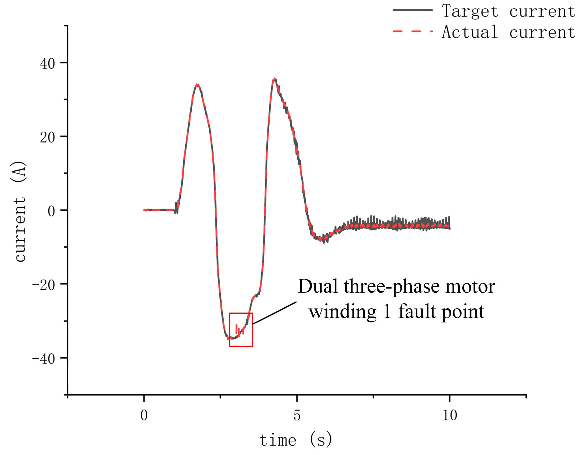
Figure 31.
Torque current output of dual three-phase motors under fault-tolerant control during fault-tolerance experiment.
In Figure 30 and Figure 31, a fault in winding 1 occurred around the 3-s mark, initiating function degradation and fault-tolerant processing. However, due to loss of the torque output capability in winding 1 of the dual three-phase motors, the steer-by-wire execution system became unbalanced, and the steering wheel slightly reversed under the action of the ground’s self-aligning torque. At that time, the torque output current of the dual three-phase motors was also disturbed. After the fault-tolerant processing was completed, the system regained a balanced state. Since winding 1 had failed and been degraded, winding 2 took over control of the entire steering system, and the torque current gradually increased to compensate for the steering torque lost due to absence of the output from winding 1, allowing the steering system to continue its steering function. The fault-tolerant steering control algorithm is thus validated.
5. Conclusions
Through this study and hardware-in-the-loop experimental validation of the dual-redundant SBW system, the following conclusions can be drawn:
- Mathematical models of the dual three-phase permanent magnet synchronous motor in the six-phase natural stationary coordinate system and a decoupled mathematical model of the synchronous rotating coordinate system were established. Analysis of the motor model concluded that the dual three-phase permanent magnet synchronous motors model in the α–β plane is identical to the three-phase permanent magnet synchronous motor model, and its control methods can be borrowed from those of the three-phase permanent magnet synchronous motor. Additionally, the impedance in the x–y plane is very small, necessitating specialized control methods to suppress harmonic currents in the x–y plane. This research on the dual three-phase permanent magnet synchronous motors model provides an important theoretical foundation for the motor theoretical analysis and control method design in this paper.
- The torque vector-space-decoupling control of the dual three-phase motors can achieve balanced torque output without torque interference in the dual-redundancy SBW system during redundancy operation; after a system fault occurs, the steering system properly executes fault-tolerant functions, maintaining normal operation.
- Rapid and smooth degradation–reconfiguration control can suppress increase in tracking errors after a system fault occurs and quickly and smoothly eliminate errors after a steering gear degradation, restoring steering function to the pre-fault tracking state.
- Rapid torque compensation and degradation–reconfiguration control can quickly compensate for loss of torque after a degradation in steering gear, restoring control and allowing the driver’s sense of force to return to the pre-fault state, ensuring the ability to steer normally after a fault.
Author Contributions
Conceptualization, M.G.; methodology, B.Q. and K.W.; software, K.W.; validation, M.G., B.Q. and K.W.; resources, K.W.; data curation, K.W.; writing—origin draft preparation, K.W.; writing—review and editing, M.G.; visualization, K.W. All authors have read and agreed to the published version of the manuscript.
Funding
Industrialization Project of Automotive Intelligent Suspension System of Shandong Province (2023CXGC010211).
Data Availability Statement
The original contributions presented in the study are included in the article; further inquiries can be directed to the corresponding author/s.
Conflicts of Interest
The authors declare no conflicts of interest.
References
- Huang, C.; Li, L. Architectural Design and Analysis of a Steer-by-Wire System in View of Functional Safety Concept. Reliab. Eng. Syst. Saf. 2020, 198, 106822. [Google Scholar] [CrossRef]
- Zheng, B.; Altemare, C.; Anwar, C. Fault Tolerant Steer-by-Wire Road Wheel Control System. Proc. Am. Control Conf. 2005, 3, 1619–1624. [Google Scholar] [CrossRef]
- Yao, Y.; Daugherty, B. Control Method of Dual Motor-Based Steer-by-Wire System. SAE Trans. 2007, 116, 354–361. [Google Scholar]
- Lin, H.; Dai, Z.; Ma, D. Research on Winding Current Balance Control Strategy for Dual—Redundancy Rudder System. Small Spec. Electr. Mach. 2012, 40, 10–13. [Google Scholar]
- Zhou, C.; Su, J.; Yang, G.; Yang, J. Vector Control of Dual Three-Phase PMSM Based on Double Zero-Sequence Voltage Injection PWM Strategy. Proc. CSEE 2015, 35, 2522–2533. [Google Scholar] [CrossRef]
- Ma, R.; Liu, W.; Yang, Y. Modeling and redundancy control of dual-redundancy brushless DC motor. Small Spec. Electr. Mach. 2008, 1, 32–35. [Google Scholar]
- Sohel, A.; Chen, L. An Analytical Redundancy-Based Fault Detection and Isolation Algorithm for a Road-Wheel Control Subsystem in a Steer-By-Wire System. IEEE Trans. Veh. Technol. 2007, 56, 2859–2869. [Google Scholar] [CrossRef]
- Sohel, A.; Niu, W. A Nonlinear Observer Based Analytical Redundancy for Predictive Fault Tolerant Control of a Steer-by-Wire System. Asian J. Control 2014, 16, 321–334. [Google Scholar] [CrossRef]
- Hasan, M.; Anwar, S. Sliding Mode Observer and Long Range Prediction Based Fault Tolerant Control of a Steer-by-Wire Equipped Vehicle; SAE Technical Paper; SAE International: Warrendale, PA, USA, 2008; p. 16. [Google Scholar] [CrossRef]
- Mi, J.; Wang, T.; Cai, Z.; Lian, X. Current balance duaFredundancy control of duaFredundant steering gears in a steer-by-wire system. J. Tsinghua Univ. Sci. Technol. 2021, 61, 898–905. [Google Scholar] [CrossRef]
- Wang, X. Research on Fault Diagnosis and Fault-Tolerant Control of Dual Three-Phase Pmsm Drive System. Doctoral Dissertation, SEU Southeast University, Nanjing, China, 2022. [Google Scholar]
- Bojoi, R.; Lazzari, M.; Profumo, F.; Tenconi, A. Digital Field-Oriented Control for Dual Three-Phase Induction Motor Drives. IEEE Trans. Ind. Appl. 2003, 39, 752–760. [Google Scholar] [CrossRef]
- Bhattacharya, S.; Mascarella, D.; Joos, G.; Cyr, J.-M.; Xu, J. A Dual Three-Level T-NPC Inverter for High-Power Traction Applications. IEEE J. Emerg. Sel. Top. Power Electron. 2016, 4, 668–678. [Google Scholar] [CrossRef]
- Dordevic, O.; Jones, M.; Levi, E. A Comparison of Carrier-Based and Space Vector PWM Techniques for Three-Level Five-Phase Voltage Source Inverters. IEEE Trans Ind. Inform. 2013, 9, 609–619. [Google Scholar] [CrossRef]
- Bodo, N.; Levi, E.; Jones, M. Investigation of Carrier-Based PWM Techniques for a Five-Phase Open-End Winding Drive Topology. IEEE Trans. Ind. Electron. 2013, 60, 2054–2065. [Google Scholar] [CrossRef]
- Abdel-Khalik, A.S.; Mostafa Gadoue, S.; Masoud, M.I.; Wiliams, B.W. Optimum Flux Distribution With Harmonic Injection for a Multiphase Induction Machine Using Genetic Algorithms. IEEE Trans. Energy Convers. 2011, 26, 501–512. [Google Scholar] [CrossRef]
- Hoang, K.D.; Ren, Y.; Zhu, Z.-Q.; Foster, M. Modified Switching-Table Strategy for Reduction of Current Harmonics in Direct Torque Controlled Dual-Three-Phase Permanent Magnet Synchronous Machine Drives. IET Electr. Power Appl. 2015, 9, 10–19. [Google Scholar] [CrossRef]
- Rodriguez, J.; Kazmierkowski, M.P.; Espinoza, J.R.; Zanchetta, P.; Abu-Rub, H.; Young, H.A.; Rojas, C.A. State of the Art of Finite Control Set Model Predictive Control in Power Electronics. IEEE Trans. Ind. Inform. 2013, 9, 1003–1016. [Google Scholar] [CrossRef]
- Kouro, S.; Cortes, P.; Vargas, R.; Ammann, U.; Rodriguez, J. Model Predictive Control—A Simple and Powerful Method to Control Power Converters. IEEE Trans. Ind. Electron. 2009, 56, 1826–1838. [Google Scholar] [CrossRef]
- Hua, W.; Chen, F.; Huang, W.; Zhang, G.; Wang, W.; Xia, W. Multivector-Based Model Predictive Control With Geometric Solution of a Five-Phase Flux-Switching Permanent Magnet Motor. IEEE Trans. Ind. Electron. 2020, 67, 10035–10045. [Google Scholar] [CrossRef]
- Najafabadi, T.A.; Salmasi, F.R.; Jabehdar-Maralani, P. Detection and Isolation of Speed-, DC-Link Voltage-, and Current-Sensor Faults Based on an Adaptive Observer in Induction-Motor Drives. IEEE Trans. Ind. Electron. 2011, 58, 1662–1672. [Google Scholar] [CrossRef]
- Foo, G.H.B.; Zhang, X.; Vilathgamuwa, D.M. A Sensor Fault Detection and Isolation Method in Interior Permanent-Magnet Synchronous Motor Drives Based on an Extended Kalman Filter. IEEE Trans. Ind. Electron. 2013, 60, 3485–3495. [Google Scholar] [CrossRef]
- Parsa, L.; Toliyat, H.A. Sensorless Direct Torque Control of Five-Phase Interior Permanent-Magnet Motor Drives. IEEE Trans. Ind. Appl. 2007, 43, 952–959. [Google Scholar] [CrossRef]


Disclaimer/Publisher’s Note: The statements, opinions and data contained in all publications are solely those of the individual author(s) and contributor(s) and not of MDPI and/or the editor(s). MDPI and/or the editor(s) disclaim responsibility for any injury to people or property resulting from any ideas, methods, instructions or products referred to in the content. |
© 2024 by the authors. Licensee MDPI, Basel, Switzerland. This article is an open access article distributed under the terms and conditions of the Creative Commons Attribution (CC BY) license (https://creativecommons.org/licenses/by/4.0/).