Active Disturbance Rejection for Linear Induction Motors: A High-Order Sliding-Mode-Observer-Based Twisting Controller

Abstract

This paper presents a twisting controller (TC) based on a high-order sliding mode observer (HOSMO) for linear induction motors (LIMs), accounting for dynamic end effects. Based on the LIM model in the field-oriented frame, two extended subsystems are developed: a velocity extended model and a flux extended model. Using these models, two HOSMOs are designed to estimate the disturbances in each subsystem. The HOSMO outputs are then used for disturbance rejection, resulting in two second-order systems with small bounded disturbances. Two TCs are subsequently implemented to achieve finite-time velocity and flux tracking of the LIM. The primary advantage of this strategy lies in its ability to reduce chattering through active disturbance rejection. Hardware-in-the-loop (HIL) experiments validate the effectiveness of the proposed TC-HOSMO scheme.

1. Introduction

With increasing competition in science and technology, the advancement level of electric drive systems directly reflects a country’s technological development [1]. As industrial control fields develop rapidly, the requirements for controlling electric drive systems have become increasingly demanding. As the core component of electric drive systems, the importance of motors is self-evident. In recent years, electric motor design and performance have been developing toward simpler and more efficient solutions [2]. Among various types, linear induction motors have gained widespread attention both domestically and internationally due to their simple mechanical structure and elimination of intermediate conversion units [3]. Compared to rotary induction motors, linear induction motors offer longer lifespans, enhanced climbing capabilities, greater flexibility in circuit design, and eliminate the need for intermediate conversion units [4,5].

However, compared to rotary induction motors, linear induction motors have inherent structural asymmetry. The dynamic end effect arises when the primary (analogous to the stator in rotary induction motors) and the secondary (analogous to the rotor) move relative to each other, and this effect becomes more pronounced as the motor speed increases [6,7]. This dynamic end effect significantly increases the model’s non-linearity and complexity, making high-precision control of linear induction motors more challenging [8,9].

Considering the influence of dynamic end effects, various control methods have been applied to LIMs, including field-oriented control techniques [10,11] and combined vector and direct thrust control methods [12]. However, these controllers exhibit relatively slow dynamic response. To address this limitation, Pucci proposed an input-output feedback linearization (FL) control strategy to enhance dynamic response performance [13]. This FL method extends control strategies from rotary to linear induction motors; however, the implementation of the final controller needs multiple transformations, leading to a significant increase in computational complexity. In practical applications, LIM parameters are affected by physical factors such as temperature and humidity [14]. The aforementioned controllers rely on accurate motor parameter information to ensure optimal control performance but struggle to maintain robustness in the presence of parameter variations or system uncertainties.

When significant uncertainties exist in industrial applications, sliding mode control theory serves as an effective solution [15,16,17]. These controllers can accurately compensate for matched uncertainties by maintaining appropriately chosen sliding variables at zero, though this theoretically requires infinite switching frequency. Among the sliding mode techniques, twisting algorithms ensure that both the expected output and its first derivative converge to zero in finite time, despite bounded perturbations [18,19]. Unlike traditional sliding mode controllers, twisting algorithms eliminate the need for sliding plane design in systems with a relative order of two [20,21].

However, the direct application of the TC technique in LIM systems leads to severe chattering phenomena. To address this issue and reduce chattering, total disturbance can be compensated through observer implementation. Among state observer techniques, the extended state observer stands as one of the most effective tools. Two linear extended state observers (LESOs) have been implemented in extended models to estimate redefined state variables and their first-time derivatives [22]. LESOs ensure asymptotic convergence of estimation errors to zero [23]. However, this method fails to guarantee adequate estimation performance under parameter uncertainty. To overcome this limitation, the super twisting observer (STO) was developed and has found wide application in various industrial settings [24]. Meanwhile, HOSMO was proposed for high-order derivative estimation. This observer shares characteristics with STO and has been widely adopted across various fields [25,26,27,28,29].

As a key power conversion device, LIM plays an important role in high-speed rail transit, industrial automation and other fields. However, its control performance is easily affected by external disturbances and internal parameter changes. To overcome this challenge, researchers introduced the auto-disturbance rejection control (ADRC) strategy, in which the twisting controller based on the high order sliding mode observer (TC-HOSMO) attracted much attention due to its high robustness and fast response ability to the disturbance. This research aims to design an efficient disturbance suppression scheme by combining the advantages of ADRC and TC to improve the control accuracy and stability of LIMs, thus meeting the requirements of high-performance applications.

This paper applies a TC-HOSMO to LIM systems, considering dynamic end effects. The main contributions are as follows: the total disturbances $f_1$ and $f_2$ in the two extended models are precisely estimated using HOSMO in finite time, and the TC-HOSMO scheme enables LIM to track the desired signals with reduced chattering in finite time despite bounded disturbances.

The remainder of this paper is organized as follows. Section 2 presents the space vector state model of LIMs, including end effects. Section 3, which constitutes the core contribution, describes the TC based on HOSMO law. This section consists of three parts: the development of two extended models, the design of HOSMOs for these models, and the proposal of a TC strategy to meet the specified requirements for flux linkage and velocity control. Section 4 demonstrates the effectiveness of the proposed TC-HOSMO technique using HIL experiments. Section 5 concludes the paper.

2. Space-Vector State Model of LIM with Dynamic End Effects

The TC-HOSMO design for LIM is based on voltage equations considering dynamic end effects, as presented in [22]. The model is established in a reference frame rotating at the induced part velocity, with the direct axis d aligned with the induced part flux vector. Following [9], the state equations are as follows:

$${\displaystyle \frac{d{i}_{ds}}{dt}}=-\gamma i_{ds}+{\displaystyle \frac{n_p\pi }{h}}v{i}_{qs}+\alpha {\displaystyle \frac{{\widehat{L}}_m{i}_{qs}^2}{{\psi }_r}}+\beta \alpha {\psi }_r+{\displaystyle \frac{u_{ds}}{\widehat{\sigma }{\widehat{L}}_s}}$$

(1)

$${\displaystyle \frac{d{i}_{qs}}{dt}}=-\gamma i_{qs}-{\displaystyle \frac{n_p\pi }{h}}v(i_{ds}+\beta {\psi }_r)-{\displaystyle \frac{\alpha {\widehat{L}}_m{i}_{ds}{i}_{qs}}{{\psi }_r}}+{\displaystyle \frac{u_{qs}}{\widehat{\sigma }{\widehat{L}}_s}}$$

(2)

$${\displaystyle \frac{d{\psi }_r}{dt}}=-(\alpha -\eta ){\psi }_r+\alpha {\widehat{L}}_m{i}_{ds}$$

(3)

$${\displaystyle \frac{d\rho }{dt}}={\displaystyle \frac{n_p\pi }{h}}v+{\displaystyle \frac{\alpha {\widehat{L}}_m{i}_{qs}}{|{\psi }_r|}}$$

(4)

$${\displaystyle \frac{dv}{dt}}=\mu \left({\psi }_r{i}_{qs}\right)-{\displaystyle \frac{F_{eb}}{M}}-{\displaystyle \frac{F_r}{M}}$$

(5)

$$F_{eb}=\vartheta [{\psi }_r^2+L_{\sigma r}^2(i_{ds}^2+i_{qs}^2)+L_{\sigma r}\left({\psi }_r{i}_{ds}\right)]$$

(6)

where ${\psi }_r={\psi }_{dr}$, ${\psi }_{qr}=0$. The system parameters are defined as follows:

$$\begin{array}{cc}\hfill \alpha & =({\displaystyle \frac{1}{{\widehat{T}}_r}}-{\displaystyle \frac{{\widehat{R}}_r}{{\widehat{L}}_m}}),\beta ={\displaystyle \frac{{\widehat{L}}_m}{\widehat{\sigma }{\widehat{L}}_s{\widehat{L}}_r}},\eta =-{\displaystyle \frac{{\widehat{R}}_r}{{\widehat{L}}_m}}\hfill \\ \hfill \mu & ={\displaystyle \frac{3n_p\pi {\widehat{L}}_m}{2Mh{\widehat{L}}_r}},\vartheta =\mathrm{sign}\left(v\right){\displaystyle \frac{3}{2}}{\displaystyle \frac{L_r}{{\widehat{L}}_r^2}}{\displaystyle \frac{1-e^{-Q}}{2n_{p}h}}\hfill \\ \hfill \gamma & ={\displaystyle \frac{1}{\widehat{\sigma }{\widehat{L}}_s}}[R_s+{\widehat{R}}_r(1-{\displaystyle \frac{{\widehat{L}}_m}{{\widehat{L}}_r}})+{\displaystyle \frac{{\widehat{L}}_m}{{\widehat{L}}_r}}({\displaystyle \frac{{\widehat{L}}_m}{{\widehat{T}}_r}}-{\widehat{R}}_r)]\hfill \end{array}$$

with auxiliary variables:

$$\begin{array}{cc}\hfill Q& ={\displaystyle \frac{{\tau }_m{R}_r}{(L_m+L_{\sigma r})v}},f\left(Q\right)={\displaystyle \frac{1-e^{-Q}}{Q}}\hfill \\ \hfill {\widehat{L}}_s& =L_{\sigma s}+{\widehat{L}}_m,{\widehat{L}}_r=L_{\sigma r}+{\widehat{L}}_m\hfill \\ \hfill {\widehat{L}}_m& =L_m[1-f\left(Q\right)],{\widehat{R}}_r=R_{r}f\left(Q\right)\hfill \\ \hfill {\widehat{T}}_r& ={\displaystyle \frac{{\widehat{L}}_r}{R_r+{\widehat{R}}_r}},\widehat{\sigma }=1-{\displaystyle \frac{{\widehat{L}}_m^2}{{\widehat{L}}_s{\widehat{L}}_r}}\hfill \end{array}$$

The symbols are defined in

Table 1. Linear Induction Motor Symbols.

Symbol	Description
$u_{ds},u_{qs}$	Inductor voltages
$i_{ds},i_{qs}$	Inductor currents
${\psi }_{ds},{\psi }_{qs}$	Induced part fluxes
$F_e,F_{eb},F_r$	Electromagnetic thrust, braking thrust, load thrust
$L_s,L_r,L_m$	Inductor inductance, induced inductance
${\tau }_m$	Inductor length
$R_s,R_r$	Inductor resistance, induced resistance
$T_r$	Induced part time constant
${\omega }_r$	Induced part electrical angular speed
$\rho$	Induced part flux space-vector angle
$v,a$	LIM speed, LIM acceleration
$\sigma$	Total leakage factor
$n_p$	Pole-pairs number
h	Pole pitch
M	Motor mass

. Unlike rotary induction motors where these parameters remain constant, LIM parameters (denoted with “^”) are velocity-dependent and time-varying due to the end effects, as detailed in [22]. Figure 1 illustrates how these parameters vary with LIM velocity.

3. Terminal Convergent Control Based on HOSMO

This section presents a TC-HOSMO design for the LIM system based on an $(n+1)$-order model, where n denotes the order of the controlled system. The approach introduces additional state variables that encompass all nonlinear terms dependent on the LIM system’s states and parameters, including external disturbances, collectively termed the total disturbance. The LIM model is transformed into a canonical form comprising cascaded integrators, with the final equation describing the total perturbation dynamics. Two HOSMOs are then designed to estimate these total disturbances, enabling the implementation of the TC strategy.

3.1. Extended Models

Two extended models are developed: the flux extended model an d the velocity extended model. The flux model captures the dynamics of the direct component of the inductance current and the induced part ofmagnetic flux, while the velocity model describes the quadrature current component and velocity dynamics. Both models are derived from Equations (1)–(6).

3.1.1. Flux Extended Model

Following the linearization approach in [13], we define state variables $x_{\psi 1}={\psi }_r$ and $x_{\psi 2}={\dot{\psi }}_r$. The flux dynamics can be expressed as:

$$\begin{array}{cc}\hfill {\dot{x}}_{\psi 1}& =x_{\psi 2}\hfill \\ \hfill {\dot{x}}_{\psi 2}& =f_1+g_1{u}_{ds}\hfill \end{array}$$

(7)

where $f_1$ represents the total flux disturbance:

$$\begin{array}{cc}\hfill f_1=& -q_1{\psi }_r+{(\alpha -\eta )}^2{\psi }_r-\alpha {\widehat{L}}_m(\alpha -\eta )i_{ds}\hfill \\ \hfill & +q_2{i}_{ds}-\alpha {\widehat{L}}_m\gamma i_{ds}+\alpha {\widehat{L}}_m{\displaystyle \frac{n_p\pi }{h}}v{i}_{qs}\hfill \\ \hfill & +{\displaystyle \frac{{\alpha }^2{\widehat{L}}_m^2{i}_{qs}^2}{|{\psi }_r|}}+{\widehat{L}}_m\beta \alpha {\psi }_r\hfill \end{array}$$

(8)

The parameters $q_1$ and $q_2$ are defined as follows:

$$\begin{array}{cc}\hfill q_1=& {\displaystyle \frac{R_r{\widehat{L}}_r+R_r{L}_m(1+f\left(Q\right))}{{\widehat{L}}_r^2}}\hfill \\ \hfill & ·{\displaystyle \frac{T_{r}a}{{\tau }_m}}\left[1-\left(1+{\displaystyle \frac{{\tau }_m}{T_{r}v}}\right)e^{-{\displaystyle \frac{{\tau }_m}{T_{r}v}}}\right]\hfill \end{array}$$

(9)

$$\begin{array}{cc}\hfill q_2=& R_r\left[{\displaystyle \frac{L_m}{{\widehat{L}}_r^2}}(1+f^2\left(Q\right))+1-2{\displaystyle \frac{L_{m}f\left(Q\right)}{{\widehat{L}}_r}}\right]\hfill \\ \hfill & ·{\displaystyle \frac{T_{r}a}{{\tau }_m}}\left[1-\left(1+{\displaystyle \frac{{\tau }_m}{T_{r}v}}\right)e^{-{\displaystyle \frac{{\tau }_m}{T_{r}v}}}\right]\hfill \end{array}$$

(10)

where $Q={\displaystyle \frac{{\tau }_m{R}_r}{(L_m+L_{\sigma r})v}}$, $f\left(Q\right)={\displaystyle \frac{1-e^{-Q}}{Q}}$, and $g_1={\displaystyle \frac{\alpha {\widehat{L}}_m}{\widehat{\sigma }{\widehat{L}}_s}}$.

Introducing a new state variable $x_{\psi 3}=f_1$, the complete flux extended model becomes:

$$\begin{array}{cc}\hfill {\dot{x}}_{\psi 1}& =x_{\psi 2}\hfill \\ \hfill {\dot{x}}_{\psi 2}& =x_{\psi 3}+g_1{u}_{ds}\hfill \\ \hfill {\dot{x}}_{\psi 3}& ={\dot{f}}_1\hfill \end{array}$$

(11)

3.1.2. Extended Velocity Model

Similar to the flux model extension, we develop the velocity model with LIM velocity as the measured output variable. Based on Equations (1)–(5) and following [13], we define state variables $x_{v1}=v$ and $x_{v2}=\dot{v}=a$. The velocity dynamics can be expressed as follows:

$$\begin{array}{cc}\hfill {\dot{x}}_{v1}& =x_{v2}\hfill \\ \hfill {\dot{x}}_{v2}& =f_2+g_2{u}_{qs}\hfill \end{array}$$

(12)

where $f_2$ represents the total velocity disturbance:

$$\begin{array}{cc}\hfill f_2=& (q_3-\mu (\alpha -\eta )){\psi }_r{i}_{qs}+\mu \alpha {\widehat{L}}_m{i}_{ds}{i}_{qs}-\gamma \mu {\psi }_r{i}_{qs}\hfill \\ \hfill & +(q_4-2{\displaystyle \frac{\vartheta }{M}}(\alpha -\eta )){\psi }_r^2+{\displaystyle \frac{\alpha \vartheta }{M}}{\widehat{L}}_m{i}_{ds}\hfill \\ \hfill & +L_{\sigma r}^2(q_2-2{\displaystyle \frac{\gamma \vartheta }{M}})i_{qs}^2\hfill \\ \hfill & -(\mu {\psi }_r+2{\displaystyle \frac{\vartheta }{M}}{L}_{\sigma r}^2)({\displaystyle \frac{n_p\pi }{h}}v{i}_{ds}\hfill \\ \hfill & +{\displaystyle \frac{{\alpha }^2{\widehat{L}}_m^2{i}_{qs}{i}_{ds}}{|{\psi }_r|}}+\beta {\displaystyle \frac{n_p\pi }{h}}v{\psi }_r-{\displaystyle \frac{{\dot{F}}_r}{M}})\hfill \end{array}$$

(13)

The parameters $q_3$ and $q_4$ are defined as follows:

$$\begin{array}{cc}\hfill q_3=& {\displaystyle \frac{3n_p\pi }{2hM}}(-{\displaystyle \frac{L_{\sigma r}{L}_m}{{\widehat{L}}_r^2}}{\displaystyle \frac{T_{r}a}{{\tau }_m}}[1-(1+{\displaystyle \frac{{\tau }_m}{T_{r}v}})e^{-{\displaystyle \frac{{\tau }_m}{T_{r}v}}}])\hfill \end{array}$$

(14)

$$\begin{array}{cc}\hfill q_4=& {\displaystyle \frac{3L_r}{2{\widehat{L}}_r^2{n}_{p}hM}}{\displaystyle \frac{a}{v}}[{\displaystyle \frac{L_m}{{\widehat{L}}_r^2}}(1-e^{-Q})(f\left(Q\right)-e^{-Q})\hfill \\ \hfill & ·({\widehat{L}}_r-L_{m}f\left(Q\right))-Q{e}^{-Q}]\hfill \end{array}$$

(15)

where $Q={\displaystyle \frac{{\tau }_m{R}_r}{(L_m+L_{\sigma r})v}}$, $f\left(Q\right)={\displaystyle \frac{1-e^{-Q}}{Q}}$, and $g_2={\displaystyle \frac{\mu {\psi }_r+2\frac{\vartheta }{M}{L}_{\sigma r}^2}{\widehat{\sigma }{\widehat{L}}_s}}$.

Introducing a new state variable $x_{v3}=f_2$, the complete velocity extended model becomes:

$$\begin{array}{cc}\hfill {\dot{x}}_{v1}& =x_{v2}\hfill \\ \hfill {\dot{x}}_{v2}& =x_{v3}+g_2{u}_{qs}\hfill \\ \hfill {\dot{x}}_{v3}& ={\dot{f}}_2\hfill \end{array}$$

(16)

Parameters $q_1$, $q_2$, $q_3$, and $q_4$ are functions of LIM velocity v and acceleration a, as illustrated in Figure 2.

3.2. High-Order Sliding Mode Observer Design

This section presents the design of two HOSMOs for estimating the total disturbances in the extended flux model (7) and velocity model (12). The observers are structured as follows:

3.2.1. Observer Equations

For the flux subsystem:

$$\begin{array}{cc}\hfill {\dot{\widehat{x}}}_{\psi 1}& ={\widehat{x}}_{\psi 2}+{\lambda }_{\psi 1}{\left|{\tilde{x}}_{\psi 1}\right|}^{2/3}\mathrm{sign}\left({\tilde{x}}_{\psi 1}\right)\hfill \\ \hfill {\dot{\widehat{x}}}_{\psi 2}& ={\widehat{x}}_{\psi 3}+{\lambda }_{\psi 2}{\left|{\tilde{x}}_{\psi 1}\right|}^{1/3}\mathrm{sign}\left({\tilde{x}}_{\psi 1}\right)+g_1{u}_{ds}\hfill \\ \hfill {\dot{\widehat{x}}}_{\psi 3}& ={\lambda }_{\psi 3}\mathrm{sign}\left({\tilde{x}}_{\psi 1}\right)\hfill \end{array}$$

(17)

For the velocity subsystem:

$$\begin{array}{cc}\hfill {\dot{\widehat{x}}}_{v1}& ={\widehat{x}}_{v2}+{\lambda }_{v1}{\left|{\tilde{x}}_{v1}\right|}^{2/3}\mathrm{sign}\left({\tilde{x}}_{v1}\right)\hfill \\ \hfill {\dot{\widehat{x}}}_{v2}& ={\widehat{x}}_{v3}+{\lambda }_{v2}{\left|{\tilde{x}}_{v1}\right|}^{1/3}\mathrm{sign}\left({\tilde{x}}_{v1}\right)+g_2{u}_{qs}\hfill \\ \hfill {\dot{\widehat{x}}}_{v3}& ={\lambda }_{v3}\mathrm{sign}\left({\tilde{x}}_{v1}\right)\hfill \end{array}$$

(18)

3.2.2. Variable Definitions

The observer variables and parameters are defined as ${\widehat{x}}_{\psi i},{\widehat{x}}_{vi}$$(i=1,2,3)$ as estimated state variables, $g_1,g_2$ as known system parameters, and ${\lambda }_{\psi i},{\lambda }_{vi}$$(i=1,2,3)$ as observer gains.

The estimation errors are defined as follows:

$$\begin{array}{cccc}\hfill {\tilde{x}}_{\psi 1}& =x_{\psi 1}-{\widehat{x}}_{\psi 1},\hfill & \hfill \hspace{1em}\hspace{1em}\hspace{1em}\hspace{1em}{\tilde{x}}_{\psi 2}& =x_{\psi 2}-{\widehat{x}}_{\psi 2}\hfill \end{array}$$

(19)

$$\begin{array}{cccc}\hfill {\tilde{x}}_{v1}& =x_{v1}-{\widehat{x}}_{v1},\hfill & \hfill \hspace{1em}\hspace{1em}\hspace{1em}\hspace{1em}{\tilde{x}}_{v2}& =x_{v2}-{\widehat{x}}_{v2}\hfill \end{array}$$

(20)

3.2.3. Error Dynamics

The estimation error dynamics are given by the follows:

For the flux subsystem:

$$\begin{array}{cc}\hfill {\dot{\tilde{x}}}_{\psi 1}& ={\tilde{x}}_{\psi 2}-{\lambda }_{\psi 1}{\left|{\tilde{x}}_{\psi 1}\right|}^{2/3}\mathrm{sign}\left({\tilde{x}}_{\psi 1}\right)\hfill \\ \hfill {\dot{\tilde{x}}}_{\psi 2}& ={\tilde{x}}_{\psi 3}-{\lambda }_{\psi 2}{\left|{\tilde{x}}_{\psi 1}\right|}^{1/3}\mathrm{sign}\left({\tilde{x}}_{\psi 1}\right)\hfill \\ \hfill {\dot{\tilde{x}}}_{\psi 3}& =-{\lambda }_{\psi 3}\mathrm{sign}\left({\tilde{x}}_{\psi 1}\right)\hfill \end{array}$$

(21)

For the velocity subsystem:

$$\begin{array}{cc}\hfill {\dot{\tilde{x}}}_{v1}& ={\tilde{x}}_{v2}-{\lambda }_{v1}{\left|{\tilde{x}}_{v1}\right|}^{2/3}\mathrm{sign}\left({\tilde{x}}_{v1}\right)\hfill \\ \hfill {\dot{\tilde{x}}}_{v2}& ={\tilde{x}}_{v3}-{\lambda }_{v2}{\left|{\tilde{x}}_{v1}\right|}^{1/3}\mathrm{sign}\left({\tilde{x}}_{v1}\right)\hfill \\ \hfill {\dot{\tilde{x}}}_{v3}& =-{\lambda }_{v3}\mathrm{sign}\left({\tilde{x}}_{v1}\right)\hfill \end{array}$$

(22)

3.2.4. Extended Error Dynamics

To complete the error analysis, we introduce additional estimation error variables:

$$\begin{array}{cc}\hfill {\tilde{x}}_{\psi 3}& =f_1-{\widehat{x}}_{\psi 3}\hfill \end{array}$$

(23)

$$\begin{array}{cc}\hfill {\tilde{x}}_{v3}& =f_2-{\widehat{x}}_{v3}\hfill \end{array}$$

(24)

The complete estimation error dynamics then become:

For the flux subsystem:

$$\begin{array}{cc}\hfill {\dot{\tilde{x}}}_{\psi 1}& ={\tilde{x}}_{\psi 2}-{\lambda }_{\psi 1}{\left|{\tilde{x}}_{\psi 1}\right|}^{2/3}\mathrm{sign}\left({\tilde{x}}_{\psi 1}\right)\hfill \\ \hfill {\dot{\tilde{x}}}_{\psi 2}& ={\tilde{x}}_{\psi 3}-{\lambda }_{\psi 2}{\left|{\tilde{x}}_{\psi 1}\right|}^{1/3}\mathrm{sign}\left({\tilde{x}}_{\psi 1}\right)\hfill \\ \hfill {\dot{\tilde{x}}}_{\psi 3}& =-{\lambda }_{\psi 3}\mathrm{sign}\left({\tilde{x}}_{\psi 1}\right)+{\dot{f}}_1\hfill \end{array}$$

(25)

For the velocity subsystem:

$$\begin{array}{cc}\hfill {\dot{\tilde{x}}}_{v1}& ={\tilde{x}}_{v2}-{\lambda }_{v1}{\left|{\tilde{x}}_{v1}\right|}^{2/3}\mathrm{sign}\left({\tilde{x}}_{v1}\right)\hfill \\ \hfill {\dot{\tilde{x}}}_{v2}& ={\tilde{x}}_{v3}-{\lambda }_{v2}{\left|{\tilde{x}}_{v1}\right|}^{1/3}\mathrm{sign}\left({\tilde{x}}_{v1}\right)\hfill \\ \hfill {\dot{\tilde{x}}}_{v3}& =-{\lambda }_{v3}\mathrm{sign}\left({\tilde{x}}_{v1}\right)+{\dot{f}}_2\hfill \end{array}$$

(26)

The disturbances are bounded by known constants:

$$\begin{array}{cc}\hfill |{\dot{f}}_1|& \le f_1^{+}\hfill \\ \hfill |{\dot{f}}_2|& \le f_2^{+}\hfill \end{array}$$

(27)

With properly designed observer gains ${\lambda }_{\psi i}$ and ${\lambda }_{vi}$ $(i=1,2,3)$, the estimation errors converge to zero in finite time $t\ge T$, yielding:

For the flux subsystem:

$$\begin{array}{cc}\hfill x_{\psi 1}& ={\widehat{x}}_{\psi 1}\hfill \\ \hfill x_{\psi 2}& ={\widehat{x}}_{\psi 2}\hfill \\ \hfill {\widehat{x}}_{\psi 3}& =f_1\hfill \end{array}$$

(28)

For the velocity subsystem:

$$\begin{array}{cc}\hfill x_{v1}& ={\widehat{x}}_{v1}\hfill \\ \hfill x_{v2}& ={\widehat{x}}_{v2}\hfill \\ \hfill {\widehat{x}}_{v3}& =f_2\hfill \end{array}$$

(29)

3.3. Terminal Convergent Control Design Based on HOSMO

3.3.1. Tracking Error Definition

The tracking errors for flux and velocity subsystems are defined as follows:

$$\begin{array}{cc}\hfill e_{\psi 1}& ={\psi }_r-{\psi }_{r,\mathrm{ref}}\hfill \end{array}$$

(30)

$$\begin{array}{cc}\hfill e_{v1}& =v-v_{\mathrm{ref}}\hfill \end{array}$$

(31)

where ${\psi }_{r,\mathrm{ref}}$ and $v_{\mathrm{ref}}$ denote the reference trajectories for rotor flux and velocity, respectively.

3.3.2. Error Dynamics

Defining the derivative tracking errors as $e_{\psi 2}={\dot{e}}_{\psi 1}$ and $e_{v2}={\dot{e}}_{v1}$, the error dynamics can be expressed as follows:

For the flux subsystem:

$$\begin{array}{cc}\hfill {\dot{e}}_{\psi 1}& =e_{\psi 2}\hfill \\ \hfill {\dot{e}}_{\psi 2}& =f_1+g_1{u}_{ds}-{\ddot{\psi }}_{r,\mathrm{ref}}\hfill \end{array}$$

(32)

For the velocity subsystem:

$$\begin{array}{cc}\hfill {\dot{e}}_{v1}& =e_{v2}\hfill \\ \hfill {\dot{e}}_{v2}& =f_2+g_2{u}_{qs}-{\ddot{v}}_{\mathrm{ref}}\hfill \end{array}$$

(33)

3.3.3. Control Law Design

The control inputs are designed as follows:

For the flux channel:

$$u_{ds}={\displaystyle \frac{1}{g_1}}(-{\widehat{x}}_{\psi 3}+{\nu }_{ds})$$

(34)

For the velocity channel:

$$u_{qs}={\displaystyle \frac{1}{g_2}}(-{\widehat{x}}_{v3}+{\nu }_{qs})$$

(35)

where ${\widehat{x}}_{\psi 3}$ represents the estimated flux disturbance $f_1$, ${\widehat{x}}_{v3}$ represents the estimated velocity disturbance $f_2$, and ${\nu }_{ds},{\nu }_{qs}$ are the auxiliary control inputs to be designed.

3.3.4. Closed-Loop Error Dynamics

Substituting the control laws into the error dynamics yields:

For the flux subsystem:

$$\begin{array}{cc}\hfill {\dot{e}}_{\psi 1}& =e_{\psi 2}\hfill \\ \hfill {\dot{e}}_{\psi 2}& =-{\ddot{\psi }}_{r,\mathrm{ref}}+{\nu }_{ds}\hfill \end{array}$$

(36)

For the velocity subsystem:

$$\begin{array}{cc}\hfill {\dot{e}}_{v1}& =e_{v2}\hfill \\ \hfill {\dot{e}}_{v2}& =-{\ddot{v}}_{\mathrm{ref}}+{\nu }_{qs}\hfill \end{array}$$

(37)

Based on [30,31,32], we consider parametric uncertainties in the control gains $g_1$ and $g_2$. For the extended models of flux (11) and velocity (16), the high-order sliding mode observers provide estimates of the equivalent disturbances:

$$\begin{array}{cc}\hfill {\widehat{x}}_{\psi 3}& \approx f_1\hfill \end{array}$$

(38)

$$\begin{array}{cc}\hfill {\widehat{x}}_{v3}& \approx f_2\hfill \end{array}$$

(39)

The control gains are bounded by:

$$\begin{array}{cc}\hfill g_1& \in [g_{\mathrm{m}1},g_{\mathrm{M}1}]\hfill \end{array}$$

(40)

$$\begin{array}{cc}\hfill g_2& \in [g_{\mathrm{m}2},g_{\mathrm{M}2}]\hfill \end{array}$$

(41)

To account for these uncertainties, we define nominal gains as geometric means:

$$\begin{array}{cc}\hfill {\widehat{g}}_1& =\sqrt{g_{\mathrm{m}1}{g}_{\mathrm{M}1}}\hfill \end{array}$$

(42)

$$\begin{array}{cc}\hfill {\widehat{g}}_2& =\sqrt{g_{\mathrm{m}2}{g}_{\mathrm{M}2}}\hfill \end{array}$$

(43)

3.3.5. Modified Control Laws

The control inputs are modified from their original form in Equations (34) and (35) to:

For the flux channel:

$$u_{ds}={\displaystyle \frac{1}{{\widehat{g}}_1}}(-{\widehat{x}}_{\psi 3}+{\nu }_{ds})$$

(44)

For the velocity channel:

$$u_{qs}={\displaystyle \frac{1}{{\widehat{g}}_2}}(-{\widehat{x}}_{v3}+{\nu }_{qs})$$

(45)

3.3.6. Resulting Error Dynamics

Substituting these modified control laws into the original error dynamics (32) and (33) yields:

For the flux subsystem:

$$\begin{array}{cc}\hfill {\dot{e}}_{\psi 1}& =e_{\psi 2}\hfill \\ \hfill {\dot{e}}_{\psi 2}& =f_1-{\displaystyle \frac{g_1}{{\widehat{g}}_1}}{\widehat{x}}_{\psi 3}-{\ddot{\psi }}_{r,\mathrm{ref}}+{\displaystyle \frac{g_1}{{\widehat{g}}_1}}{\nu }_{ds}\hfill \end{array}$$

(46)

For the velocity subsystem:

$$\begin{array}{cc}\hfill {\dot{e}}_{v1}& =e_{v2}\hfill \\ \hfill {\dot{e}}_{v2}& =f_2-{\displaystyle \frac{g_2}{{\widehat{g}}_2}}{\widehat{x}}_{v3}-{\ddot{v}}_{\mathrm{ref}}+{\displaystyle \frac{g_2}{{\widehat{g}}_2}}{\nu }_{qs}\hfill \end{array}$$

(47)

If ${\widehat{g}}_1=g_1$ and ${\widehat{g}}_2=g_2$, the above two subsystems reduce to control models (36) and (37). However, when ${\widehat{g}}_1\ne g_1$ and ${\widehat{g}}_2\ne g_2$ (with $g_1\approx {\widehat{g}}_1$ and $g_2\approx {\widehat{g}}_2$), the dynamics become the following:

For the flux subsystem:

$$\begin{array}{cc}\hfill {\dot{e}}_{\psi 1}& =e_{\psi 2}\hfill \\ \hfill {\dot{e}}_{\psi 2}& =f_1\left(1-{\displaystyle \frac{g_1}{{\widehat{g}}_1}}\right)-{\ddot{\psi }}_{r,\mathrm{ref}}+{\displaystyle \frac{g_1}{{\widehat{g}}_1}}{\nu }_{ds}\hfill \end{array}$$

(48)

For the velocity subsystem:

$$\begin{array}{cc}\hfill {\dot{e}}_{v1}& =e_{v2}\hfill \\ \hfill {\dot{e}}_{v2}& =f_2\left(1-{\displaystyle \frac{g_2}{{\widehat{g}}_2}}\right)-{\ddot{v}}_{\mathrm{ref}}+{\displaystyle \frac{g_2}{{\widehat{g}}_2}}{\nu }_{qs}\hfill \end{array}$$

(49)

These equations can be written in compact form:

For the flux subsystem:

$$\begin{array}{cc}\hfill {\dot{e}}_{\psi 1}& =e_{\psi 2}\hfill \\ \hfill {\dot{e}}_{\psi 2}& ={\zeta }_1+{\displaystyle \frac{g_1}{{\widehat{g}}_1}}{\nu }_{ds}\hfill \end{array}$$

(50)

For the velocity subsystem:

$$\begin{array}{cc}\hfill {\dot{e}}_{v1}& =e_{v2}\hfill \\ \hfill {\dot{e}}_{v2}& ={\zeta }_2+{\displaystyle \frac{g_2}{{\widehat{g}}_2}}{\nu }_{qs}\hfill \end{array}$$

(51)

where ${\zeta }_1=f_1(1-g_1/{\widehat{g}}_1)-{\ddot{\psi }}_{r,\mathrm{ref}}$ and ${\zeta }_2=f_2(1-g_2/{\widehat{g}}_2)-{\ddot{v}}_{\mathrm{ref}}$. As only the bounds of $g_1/{\widehat{g}}_1$ and $g_2/{\widehat{g}}_2$ are known, robust control techniques are required to ensure system stability.

Notice that models (50) and (51) can be expressed as second-order systems:

$${\ddot{e}}_{\psi 1}=a_{\psi }\left(t\right)+b_{\psi }\left(t\right){\nu }_{ds}$$

(52)

$${\ddot{e}}_{v1}=a_v\left(t\right)+b_v\left(t\right){\nu }_{qs}$$

(53)

where

$$\begin{array}{cccc}\hfill a_{\psi }\left(t\right)& ={\zeta }_1,\hfill & \hfill \hspace{1em}\hspace{1em}\hspace{1em}\hspace{1em}\hspace{1em}{b}_{\psi }\left(t\right)& ={\displaystyle \frac{g_1}{{\widehat{g}}_1}}\hfill \end{array}$$

(54)

$$\begin{array}{cccc}\hfill a_v\left(t\right)& ={\zeta }_2,\hfill & \hfill \hspace{1em}\hspace{1em}\hspace{1em}\hspace{1em}\hspace{1em}{b}_v\left(t\right)& ={\displaystyle \frac{g_2}{{\widehat{g}}_2}}\hfill \end{array}$$

(55)

Under the assumptions:

$$\begin{array}{ccc}\hfill |{\zeta }_1|& \le C_1,\hfill & \hfill \hspace{1em}\hspace{1em}\hspace{1em}\hspace{1em}\hspace{1em}\hspace{1em}0\le K_{m1}\le {\displaystyle \frac{g_1}{{\widehat{g}}_1}}\le K_{M1}\end{array}$$

(56)

$$\begin{array}{ccc}\hfill |{\zeta }_2|& \le C_2,\hfill & \hfill \hspace{1em}\hspace{1em}\hspace{1em}\hspace{1em}\hspace{1em}\hspace{1em}0\le K_{m2}\le {\displaystyle \frac{g_2}{{\widehat{g}}_2}}\le K_{M2}\end{array}$$

(57)

The twisting algorithm yields the following control laws:

For the flux channel:

$$\begin{array}{cc}\hfill {\nu }_{ds}& =-r_{d1}\mathrm{sign}\left(e_{\psi 1}\right)-r_{d2}\mathrm{sign}\left(e_{\psi 2}\right)\hfill \\ \hfill & =-r_{d1}\mathrm{sign}(x_{\psi 1}-x_{\psi 1,\mathrm{ref}})\hfill \\ \hfill & -r_{d2}\mathrm{sign}({\dot{x}}_{\psi 1}-{\dot{x}}_{\psi 1,\mathrm{ref}})\hfill \end{array}$$

(58)

For the velocity channel:

$$\begin{array}{cc}\hfill {\nu }_{qs}& =-r_{q1}\mathrm{sign}\left(e_{v1}\right)-r_{q2}\mathrm{sign}\left(e_{v2}\right)\hfill \\ \hfill & =-r_{q1}\mathrm{sign}(x_{v1}-x_{v1,\mathrm{ref}})\hfill \\ \hfill & -r_{q2}\mathrm{sign}({\dot{x}}_{v1}-{\dot{x}}_{v1,\mathrm{ref}})\hfill \end{array}$$

(59)

The control parameters must satisfy:

For the flux control:

$$\begin{array}{cc}\hfill K_{m1}(r_{d1}+r_{d2})-C_1& >K_{M1}(r_{d1}+r_{d2})+C_1\hfill \end{array}$$

(60)

$$\begin{array}{cc}\hfill K_{m1}(r_{d1}+r_{d2})& >C_1\hfill \end{array}$$

(61)

For the velocity control:

$$\begin{array}{cc}\hfill K_{m2}(r_{q1}+r_{q2})-C_2& >K_{M2}(r_{q1}+r_{q2})+C_2\hfill \end{array}$$

(62)

$$\begin{array}{cc}\hfill K_{m2}(r_{q1}+r_{q2})& >C_2\hfill \end{array}$$

(63)

The proposed controllers ensure finite-time convergence to the two-sliding manifolds:

$$\begin{array}{cc}\hfill e_{\psi 2}={\dot{e}}_{\psi 1}& =0\hfill \end{array}$$

(64)

$$\begin{array}{cc}\hfill e_{v2}={\dot{e}}_{v1}& =0\hfill \end{array}$$

(65)

For the detailed convergence proof, readers are referred to [20]. In practical implementations, parametric uncertainties in $g_1$ and $g_2$ affect the reduced second-order system obtained after disturbance compensation. These uncertainties necessitate the proposed robust TC to achieve a finite-time tracking performance for both velocity and flux variables.

Proposition 1.

The TC-HOSMO reduces control gains while preserving finite-time convergence, thereby achieving reduced chattering compared with classical TC.

Proof. 

Without HOSMOs, the total disturbances $f_1$ and $f_2$ cannot be estimated, eliminating the terms ${\widehat{x}}_{\psi 3}$ and ${\widehat{x}}_{v3}$ from control laws (44) and (45). The control inputs reduce to the following:

$$\begin{array}{cc}\hfill u_{ds}& ={\displaystyle \frac{1}{{\widehat{g}}_1}}{\nu }_{ds}\hfill \end{array}$$

(66)

$$\begin{array}{cc}\hfill u_{qs}& ={\displaystyle \frac{1}{{\widehat{g}}_2}}{\nu }_{qs}\hfill \end{array}$$

(67)

Consequently, control models (32) and (33) become:

For the flux subsystem:

$$\begin{array}{cc}\hfill {\dot{e}}_{\psi 1}& =e_{\psi 2}\hfill \\ \hfill {\dot{e}}_{\psi 2}& =d_1+{\displaystyle \frac{g_1}{{\widehat{g}}_1}}{\nu }_{ds}\hfill \end{array}$$

(68)

For the velocity subsystem:

$$\begin{array}{cc}\hfill {\dot{e}}_{v1}& =e_{v2}\hfill \\ \hfill {\dot{e}}_{v2}& =d_2+{\displaystyle \frac{g_2}{{\widehat{g}}_2}}{\nu }_{qs}\hfill \end{array}$$

(69)

where:

$$\begin{array}{cc}\hfill d_1& =f_1-{\ddot{\psi }}_{r,\mathrm{ref}}\hfill \end{array}$$

(70)

$$\begin{array}{cc}\hfill d_2& =f_2-{\ddot{v}}_{\mathrm{ref}}\hfill \end{array}$$

(71)

The corresponding control laws become:

For flux control:

$$\begin{array}{cc}\hfill {\nu }_{ds}& =-r_{D1}\mathrm{sign}\left(e_{\psi 1}\right)-r_{D2}\mathrm{sign}\left(e_{\psi 2}\right)\hfill \\ \hfill & =-r_{D1}\mathrm{sign}(x_{\psi 1}-x_{\psi 1,\mathrm{ref}})\hfill \\ \hfill & -r_{D2}\mathrm{sign}({\dot{x}}_{\psi 1}-{\dot{x}}_{\psi 1,\mathrm{ref}})\hfill \end{array}$$

(72)

For velocity control:

$$\begin{array}{cc}\hfill {\nu }_{qs}& =-r_{Q1}\mathrm{sign}\left(e_{v1}\right)-r_{Q2}\mathrm{sign}\left(e_{v2}\right)\hfill \\ \hfill & =-r_{Q1}\mathrm{sign}(x_{v1}-x_{v1,\mathrm{ref}})\hfill \\ \hfill & -r_{Q2}\mathrm{sign}({\dot{x}}_{v1}-{\dot{x}}_{v1,\mathrm{ref}})\hfill \end{array}$$

(73)

Given that:

$$\begin{array}{cccc}\hfill |{\zeta }_1|& \ll |d_1|,\hfill & \hfill \hspace{1em}\hspace{1em}\hspace{1em}\hspace{1em}\hspace{1em}\hspace{1em}|{\zeta }_2|& \ll |d_2|\hfill \end{array}$$

(74)

The control gains without HOSMO must be significantly larger:

$$\begin{array}{cccc}\hfill r_{D1}& \gg r_{d1},\hfill & \hfill \hspace{1em}\hspace{1em}\hspace{1em}\hspace{1em}\hspace{1em}\hspace{1em}{r}_{D2}& \gg r_{d2}\hfill \end{array}$$

(75)

$$\begin{array}{cccc}\hfill r_{Q1}& \gg r_{q1},\hfill & \hfill \hspace{1em}\hspace{1em}\hspace{1em}\hspace{1em}\hspace{1em}\hspace{1em}{r}_{Q2}& \gg r_{q2}\hfill \end{array}$$

(76)

These substantially higher gains in classical TC result in increased chattering compared with the HOSMO-based approach. □

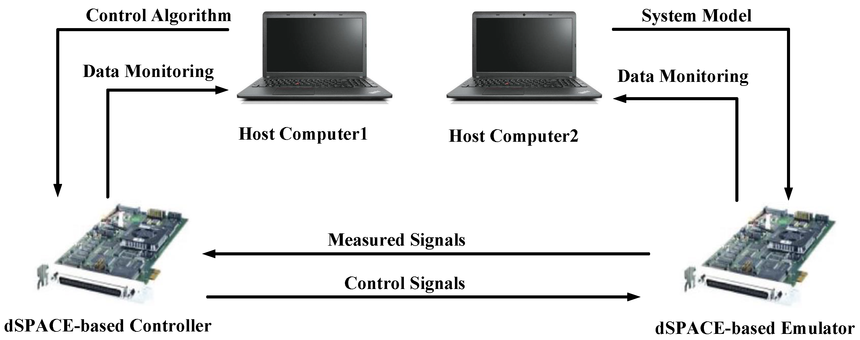
4. Hardware-in-the-Loop Experimental Validation

A dual-dSPACE HIL test platform is developed to validate the proposed TC-HOSMO strategy against classical TC, as illustrated in Figure 3. This real-time platform provides an efficient and cost-effective solution for control validation. The setup comprises two key components: dSPACE Controller and dSPACE Emulator.

• Controller dSPACE DS1104: Implements the TC-HOSMO control algorithm at 10 kHz sampling rate.
• Emulator dSPACE DS1104: Simulates the LIM drive system at 10 kHz sampling rate, incorporating:

  –

  Dynamic end-effect model (Equations (1)–(6)). The specific steps are as follows: Firstly, the LIM model is validated using experimental data to ensure its accuracy and effectiveness. Secondly, a real-time simulation environment is established based on the selected processor and I/O module. This involves implementing the system model in software code to enable real-time execution. Finally, the system under test is connected to the simulator, ensuring that all signals are transmitted accurately. The necessary communication protocols are configured to facilitate seamless data exchange between the system and the simulator.

  –

  Park’s transformation is used for voltage and current coordinate conversion between three-phase stator and rotor reference frames. The process typically consists of two stages: first, converting three-phase quantities into a stationary reference frame using Clarke’s transformation, and second, applying a rotational transformation to map these quantities into the dq frame synchronized with the rotor’s electrical position. This approach enhances dynamic performance, reduces computational complexity, and improves stability in modern motor drives, renewable energy systems, and power electronics applications. The nominal parameters of the LIM are shown in the Table 2.

Table 2. Linear Induction Motor Parameters.

Parameter	Value
Stator resistance, $R_s$	11 $\mathsf{\Omega }$
Secondary resistance, $R_r$	32.57 $\mathsf{\Omega }$
Stator inductance, $L_s$	0.6376 H
Magnetizing inductance, $L_m$	0.5175 H
Secondary inductance, $L_r$	0.7578 H
Primary mass, M	20 kg
Viscous friction coefficient, D	20 N·s/m
Number of pole pairs, $n_p$	3
Pole pitch, h	0.1 m

Table 2. Linear Induction Motor Parameters.

Parameter	Value
Stator resistance, $R_s$	11 $\mathsf{\Omega }$
Secondary resistance, $R_r$	32.57 $\mathsf{\Omega }$
Stator inductance, $L_s$	0.6376 H
Magnetizing inductance, $L_m$	0.5175 H
Secondary inductance, $L_r$	0.7578 H
Primary mass, M	20 kg
Viscous friction coefficient, D	20 N·s/m
Number of pole pairs, $n_p$	3
Pole pitch, h	0.1 m

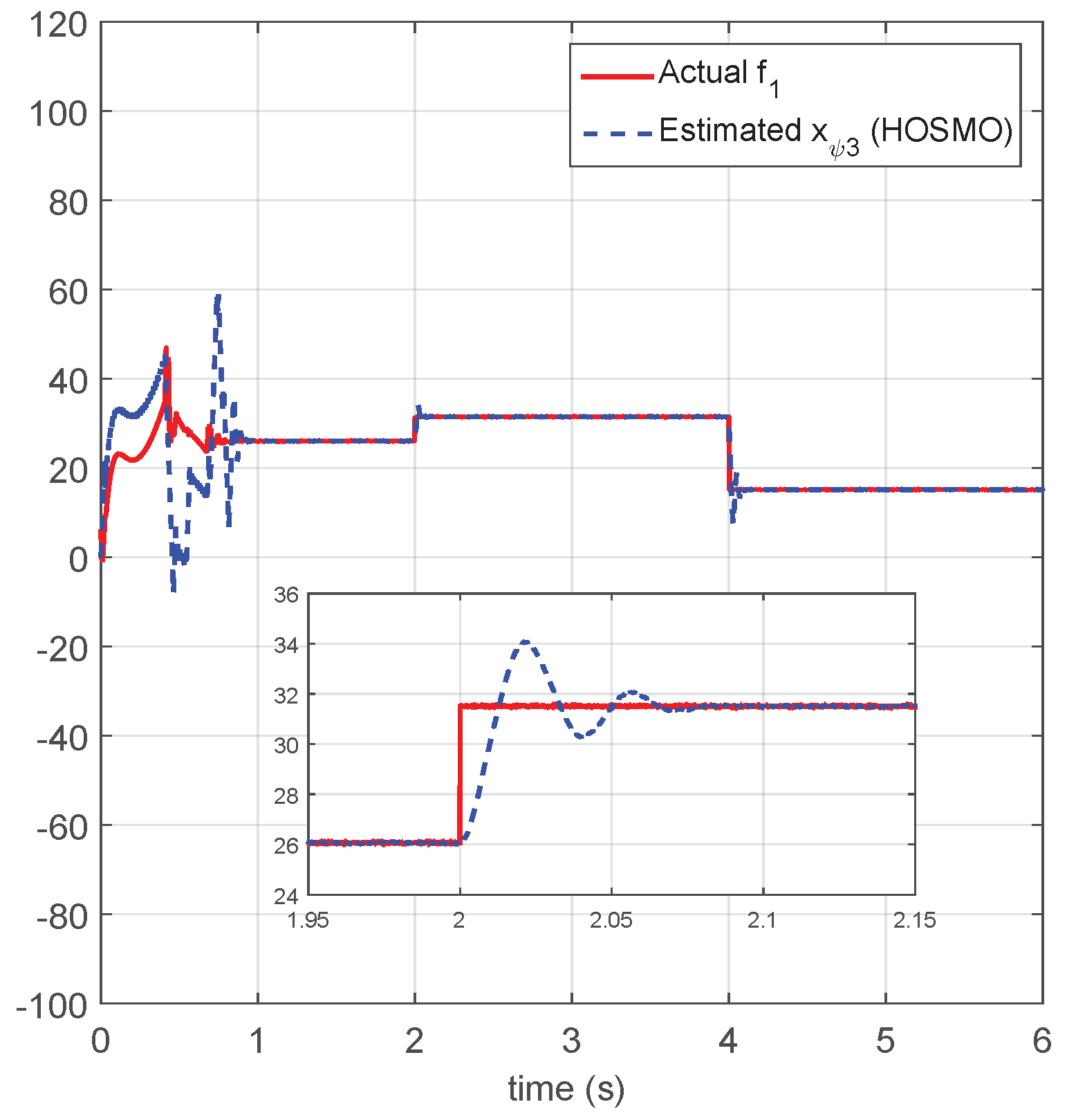
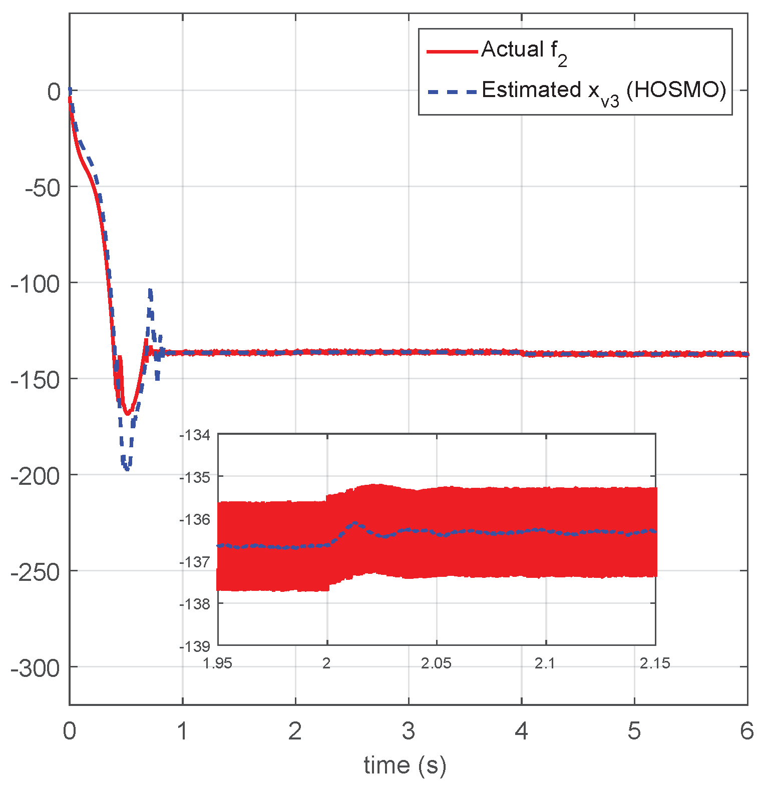
4.1. HOSMO Performance Evaluation

The HOSMO implementation uses the following gains:

$$\begin{array}{cc}\hfill \mathrm{Flux}\mathrm{observer}:& {\lambda }_{\psi 1}=1000, {\lambda }_{\psi 2}=500, {\lambda }_{\psi 3}=1000\hfill \end{array}$$

(77)

$$\begin{array}{cc}\hfill \mathrm{Velocity}\mathrm{observer}:& {\lambda }_{v1}=1000, {\lambda }_{v2}=500, {\lambda }_{v3}=1000\hfill \end{array}$$

(78)

To evaluate robustness, we introduce time-varying stator resistance perturbations:

$$\mathsf{\Delta }{R}_s=\left\{\begin{array}{cc}0,\hfill & 0\mathrm{s}\le t<2\mathrm{s}\hfill \\ -0.2R_s,\hfill & 2\mathrm{s}\le t<4\mathrm{s}\hfill \\ 0.2R_s,\hfill & 4\mathrm{s}\le t\le 6\mathrm{s}\hfill \end{array}\right.$$

(79)

where the actual stator resistance becomes ${\overline{R}}_s=R_s+\mathsf{\Delta }{R}_s$.

Figure 4 and Figure 5 demonstrate the observer’s capability to accurately reconstruct both flux and velocity disturbances ($f_1$ and $f_2$) despite parametric uncertainties. The proposed HOSMO effectively compensates for unmodeled dynamics and parameter variations through its high-gain architecture and adaptive disturbance estimation mechanism. As shown in the time-domain responses, the observer achieves precise disturbance reconstruction within finite time while maintaining robustness against variations in system parameters such as inertia and friction coefficients. Notably, the estimation errors for both flux and velocity disturbances converge to a bounded region within 1 s, demonstrating a superior transient performance. This capability remains consistent under disturbances, validating the observer’s applicability in practical scenarios with complex operating conditions. The results further highlight the observer’s ability to decouple parametric uncertainties from disturbance estimation through its innovative error injection term.

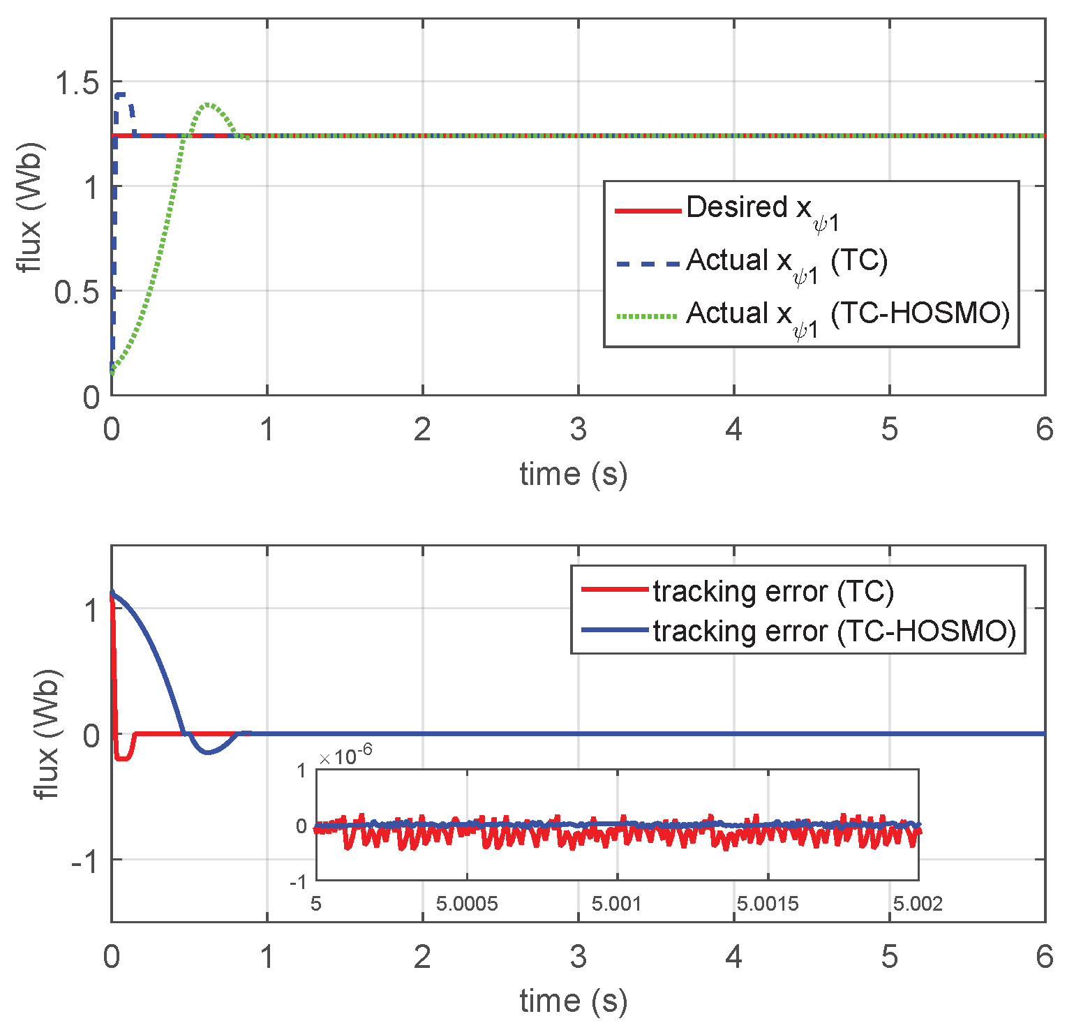
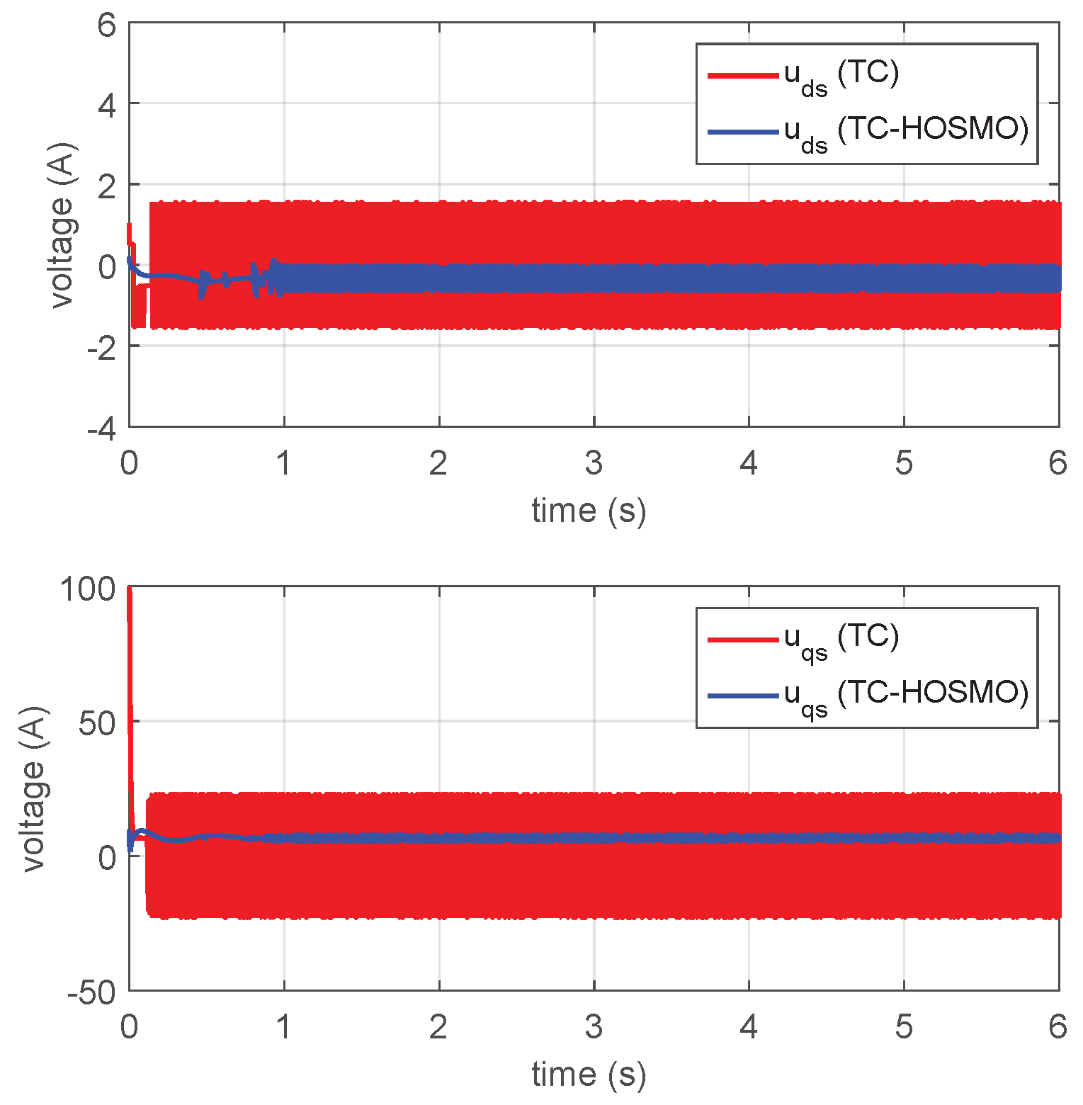
4.2. Comparative Analysis of TC-HOSMO Performance

The comparative study implements two control schemes with the following parameters:

TC-HOSMO configuration:

$$\begin{array}{cc}\hfill \mathrm{TC}\mathrm{gains}:& r_{d1}=16, r_{d2}=8, r_{q1}=16, r_{q2}=8\hfill \end{array}$$

(80)

$$\begin{array}{cc}\hfill \mathrm{HOSMO}\mathrm{gains}:& {\lambda }_{\psi 1}=1000, {\lambda }_{\psi 2}=500, {\lambda }_{\psi 3}=1000,\hfill \end{array}$$

(81)

$$\begin{array}{cc}\hfill & {\lambda }_{v1}=1000, {\lambda }_{v2}=500, {\lambda }_{v3}=1000\hfill \end{array}$$

(82)

Classical TC configuration:

$$r_{D1}=80, r_{D2}=40, r_{Q1}=320, r_{Q2}=160$$

(83)

The experimental results in Figure 6 and Figure 7 demonstrate that while both controllers achieve finite-time convergence, TC-HOSMO exhibits significantly reduced chattering. This improvement stems from its hybrid structure integrating higher-order sliding modes with a dynamic adaptive gain adjustment mechanism, which replaces discontinuous switching terms with smoothed error injection signals. Particularly, the chattering frequency spectrum reveals that TC-HOSMO attenuates high-frequency components above 1 kHz, crucially mitigating mechanical wear and sensor noise amplification in practical implementations. The reduced chattering also enhances control precision, achieving steady-state tracking errors even under parameter mismatches. Moreover, the adaptive layer embedded in TC-HOSMO dynamically modulates observer gains based on real-time disturbance estimates, effectively balancing chattering suppression and disturbance rejection robustness. These characteristics position TC-HOSMO as a superior solution for applications requiring both smooth actuation and rigorous finite-time stability guarantees.

Figure 8 reveals smoother control inputs ($u_{ds}$ and $u_{qs}$) for TC-HOSMO, attributable to HOSMO’s compensation of disturbances $f_1$ and $f_2$ in the control design. The observed reduction in input signal oscillations (quantified by standard deviation metrics) stems from the observer’s ability to preemptively counteract disturbances through its two-layer estimation architecture. This improvement is achieved through the nonlinear disturbance observer’s adaptive bandwidth modulation, significantly reducing electromagnetic interference risks. The smoothed inputs also correlate with enhanced energy efficiency, exhibiting lower Joule losses compared with discontinuous control counterparts. Such characteristics validate the integrated observer-controller structure’s effectiveness in decoupling disturbance dynamics from actuation signals, while preserving the inherent finite-time convergence properties of sliding mode control.

5. Conclusions

This paper presents a novel twisting control strategy integrated with high-order sliding mode observers for LIMs. The proposed TC-HOSMO framework explicitly addresses the dynamic end-effects by decomposing the LIM model into speed and flux-extended subsystems. Two high-order sliding mode observers are designed to achieve disturbance rejection while maintaining robustness and finite-time convergence properties. The TC are then synthesized to achieve flux and speed tracking with reduced chattering. The effectiveness of the proposed approach has been thoroughly validated through both Matlab/Simulink simulations and hardware-in-the-loop experiments. Key findings demonstrate that HOSMOs accurately estimate the total disturbances even in the presence of parametric uncertainties. Moreover, a comparative analysis reveals that the TC-HOSMO scheme achieves significantly reduced chattering compared with classical twisting control while maintaining finite-time convergence and robustness characteristics. Both theoretical analysis and experimental results validate that the proposed TC-HOSMO framework provides an effective control solution for LIM applications. In the future, ADRC will be combined with other advanced control methods (such as model predictive control and adaptive control) to form a composite control strategy to further improve the control performance of LIMs. At the same time, by optimizing the controller parameters and algorithm design, the control precision and response speed of the LIM are improved to meet the control requirements of higher precision.

References

1. Rametti, S.; Pierrejean, L.; Hodder, A.; Paolone, M. Pseudo-Three-Dimensional Analytical Model of Linear Induction Motors for High-Speed Applications. IEEE Trans. Transp. Electrif. 2024, 10, 9109–9120. [Google Scholar] [CrossRef]
2. Xiao, X.; Xu, W.; Tang, Y.; Li, W.; Dong, D.; Shangguan, Y.; Huang, S. Improved Loss Minimization Control Based on Time-Harmonic Equivalent Circuit for Linear Induction Motors Adopted to Linear Metro. IEEE Trans. Veh. Technol. 2023, 72, 8601–8612. [Google Scholar] [CrossRef]
3. Hamad, S.A.; Ghalib, M.A. Fuzzy MPPT Operation-Based Model Predictive Flux Control for Linear Induction Motors. Int. J. Hydrogen Energy 2024, 50, 1035–1044. [Google Scholar] [CrossRef]
4. Zhang, M.; Luo, S.; Liu, Y.; Zhuang, X.; Ma, W. Analysis of the Traction Forces of Two Adjacent Linear Induction Motors. Sci. Rep. 2024, 14, 26760. [Google Scholar] [CrossRef]
5. Gomes, D.R.; Chabu, I.E. A Novel Analytical Equivalent Circuit for Single-Sided Linear Induction Motors Considering Secondary Leakage Reactance. Energies 2023, 16, 1261. [Google Scholar] [CrossRef]
6. Palka, R.; Woronowicz, K. Linear Induction Motors in Transportation Systems. Energies 2021, 14, 2549. [Google Scholar] [CrossRef]
7. Sun, Z.; Xu, L.; Zhao, W.; Du, K. Comparison between Linear Induction Motor and Linear Primary Permanent Magnet Vernier Motor for Railway Transportation. In Proceedings of the 2021 13th International Symposium on Linear Drives for Industry Applications (LDIA), Wuhan, China, 1–3 July 2021; pp. 1–6. [Google Scholar]
8. Duncan, J. Linear Induction Motor-Equivalent-Circuit Model. IEE Proc. B (Electr. Power Appl.) 1983, 130, 51–57. [Google Scholar]
9. Pucci, M. State Space-Vector Model of Linear Induction Motors. IEEE Trans. Ind. Appl. 2014, 50, 195–207. [Google Scholar] [CrossRef]
10. Kang, G.; Nam, K. Field-Oriented Control Scheme for Linear Induction Motor with the End Effect. IEE Proc.-Electr. Power Appl. 2005, 152, 1565–1572. [Google Scholar] [CrossRef]
11. Pucci, M. Direct Field Oriented Control of Linear Induction Motors. Elect. Power Syst. Res. 2012, 89, 11–22. [Google Scholar] [CrossRef]
12. Karimi, H.; Vaez-Zadeh, S.; Salmasi, F.R. Combined Vector and Direct Thrust Control of Linear Induction Motors with End Effect Compensation. IEEE Trans. Energy Convers. 2016, 31, 196–205. [Google Scholar] [CrossRef]
13. Accetta, A.; Cirrincione, M.; D’Ippolito, F.; Pucci, M.; Sferlazza, A. Input–Output Feedback Linearization Control of a Linear Induction Motor Taking into Consideration Its Dynamic End-Effects and Iron Losses. IEEE Trans. Ind. Appl. 2022, 58, 3664–3673. [Google Scholar] [CrossRef]
14. Krim, S.; Gdaim, S.; Mtibaa, A.; Faouzi Mimouni, M. FPGA-Based Real-Time Implementation of a Direct Torque Control with Second-Order Sliding Mode Control and Input–Output Feedback Linearisation for an Induction Motor Drive. IET Electr. Power Appl. 2020, 14, 480–491. [Google Scholar] [CrossRef]
15. Wu, L.; Liu, J.; Vazquez, S.; Mazumder, S.K. Sliding Mode Control in Power Converters and Drives: A Review. IEEE/CAA J. Autom. Sin. 2021, 9, 392–406. [Google Scholar] [CrossRef]
16. Mousavi, Y.; Bevan, G.; Kucukdemiral, I.B.; Fekih, A. Sliding Mode Control of Wind Energy Conversion Systems: Trends and Applications. Renew. Sustain. Energy Rev. 2022, 167, 112734. [Google Scholar] [CrossRef]
17. Ye, Z.; Zhang, D.; Cheng, J.; Wu, Z.G. Event-Triggering and Quantized Sliding Mode Control of UMV Systems under DoS Attack. IEEE Trans. Veh. Technol. 2022, 71, 8199–8211. [Google Scholar] [CrossRef]
18. Hu, Q.; Han, T.; Xin, M. Three-Dimensional Guidance for Various Target Motions with Terminal Angle Constraints Using Twisting Control. IEEE Trans. Ind. Electron. 2019, 67, 1242–1253. [Google Scholar] [CrossRef]
19. Shtessel, Y.B.; Moreno, J.A.; Fridman, L.M. Twisting Sliding Mode Control with Adaptation: Lyapunov Design, Methodology and Application. Automatica 2017, 75, 229–235. [Google Scholar] [CrossRef]
20. Utkin, V.; Poznyak, A.; Orlov, Y.; Polyakov, A. Conventional and High Order Sliding Mode Control. J. Frankl. Inst. 2020, 357, 10244–10261. [Google Scholar] [CrossRef]
21. Li, B.; Gao, X.; Huang, H.; Yang, H. Improved Adaptive Twisting Sliding Mode Control for Trajectory Tracking of an AUV Subject to Uncertainties. Ocean Eng. 2024, 297, 116204. [Google Scholar] [CrossRef]
22. Huang, C.; Li, J.; Mu, S.; Yan, H. Linear Active Disturbance Rejection Control Approach for Load Frequency Control of Two-Area Interconnected Power System. Trans. Inst. Meas. Control 2019, 41, 1562–1570. [Google Scholar] [CrossRef]
23. Castillo, A.; García, P.; Sanz, R.; Albertos, P. Enhanced Extended State Observer-Based Control for Systems with Mismatched Uncertainties and Disturbances. ISA Trans. 2018, 73, 1–10. [Google Scholar] [CrossRef] [PubMed]
24. Wang, S.; Wang, H.; Tang, C.; Li, J.; Liang, D.; Qu, Y. Research on Control Strategy of Permanent Magnet Synchronous Motor Based on Fast Terminal Super-Twisting Sliding Mode Observer. IEEE Access 2024, 12, 141905–141915. [Google Scholar] [CrossRef]
25. Wang, D.; Liu, X. Sensorless Control of PMSM with Improved Adaptive Super-Twisting Sliding Mode Observer and IST-QSG. IEEE Trans. Transp. Electrif. 2024, 11, 721–731. [Google Scholar] [CrossRef]
26. Chalanga, A.; Kamal, S.; Fridman, L.M.; Bandyopadhyay, B.; Moreno, J.A. Implementation of Super-Twisting Control: Super-Twisting and Higher Order Sliding-Mode Observer-Based Approaches. IEEE Trans. Ind. Electron. 2016, 63, 3677–3685. [Google Scholar] [CrossRef]
27. Gonzalez-Hernandez, I.; Palacios, F.M.; Cruz, S.S.; Quesada, E.S.E.; Leal, R.L. Real-Time Altitude Control for a Quadrotor Helicopter Using a Super-Twisting Controller Based on High-Order Sliding Mode Observer. Int. J. Adv. Robot. Syst. 2017, 14, 1729881416687113. [Google Scholar] [CrossRef]
28. Delavari, H.; Heydarinejad, H.; Baleanu, D. Adaptive Fractional-Order Blood Glucose Regulator Based on High-Order Sliding Mode Observer. IET Syst. Biol. 2018, 13, 43–54. [Google Scholar] [CrossRef]
29. Belkhatir, Z.; Laleg-Kirati, T.M. High-Order Sliding Mode Observer for Fractional Commensurate Linear Systems with Unknown Input. Automatica 2017, 82, 209–217. [Google Scholar] [CrossRef]
30. Alonge, F.; Cirrincione, M.; D’Ippolito, F.; Pucci, M.; Sferlazza, A. Robust Active Disturbance Rejection Control of Induction Motor Systems Based on Additional Sliding-Mode Component. IEEE Trans. Ind. Electron. 2017, 64, 5608–5621. [Google Scholar] [CrossRef]
31. Madonski, R.; Shao, S.; Zhang, H.; Gao, Z.; Yang, J.; Li, S. General Error-Based Active Disturbance Rejection Control for Swift Industrial Implementations. Control Eng. Pract. 2019, 84, 218–229. [Google Scholar] [CrossRef]
32. Nigam, S.; Ajala, O.; Domínguez-García, A.D.; Sauer, P.W. Controller Hardware in the Loop Testing of Microgrid Secondary Frequency Control Schemes. Elect. Power Syst. Res. 2021, 190, 106757. [Google Scholar] [CrossRef]
Figure 1. Variation in parameters γ , α , β , η , μ , and ϑ with LIM velocity (0–5 m/s).
Actuators 14 00200 g001
Figure 2. Parameter surfaces q 1 q 4 vs. velocity (0–10 m/s) and acceleration (0–10 m/s2).
Actuators 14 00200 g002
Figure 3. Hardware-in-the-loop test bench architecture for the TC-HOSMO scheme.
Actuators 14 00200 g003
Figure 4. Experimental validation of flux-related total disturbance ( f 1 ) estimation performance.
Actuators 14 00200 g004
Figure 5. Experimental validation of velocity-related total disturbance ( f 2 ) estimation performance.
Actuators 14 00200 g005
Figure 6. Comparative analysis of flux tracking performance.
Actuators 14 00200 g006
Figure 7. Comparative analysis of velocity tracking performance.
Actuators 14 00200 g007
Figure 8. Control effort comparison: u d s and u q s trajectories.
Actuators 14 00200 g008