An Optimized Position Control via Reinforcement-Learning-Based Hybrid Structure Strategy

Abstract

Most control system implementations rely on single structures optimized for specific performance criteria through rigorous derivation. While effective for their intended purpose, such controllers often underperform in areas outside their primary optimization focus and involve performance trade-offs. A notable example is the Internal Model Principle (IMP) controller, renowned for its robustness and precision in reference tracking under periodic disturbances. However, IMP controllers exhibit poor transient-state performance, characterized by significant overshoot and oscillatory responses, which remains a persistent challenge. To address this limitation, this paper proposes a reinforcement learning (RL)-based hybrid control scheme that overcomes the trade-off in IMP controllers between achieving zero steady-state tracking error and a fast transient response. The proposed method integrates a cascade control structure, optimized for transient-state performance, with an IMP controller, optimized for robust reference tracking under sinusoidal disturbances, through switching logic governed by a Deep Q-Network model. Smooth transitions between control modes are ensured using an internal state update mechanism. The proposed approach is validated through simulations and experimental tests on a direct current (DC) motor position control system. The results demonstrate that the hybrid structure effectively resolves the trade-off associated with IMP controllers, yielding improved performance metrics, such as rapid convergence to the reference, reduced transient overshoot, and enhanced nominal performance recovery against disturbances.

1. Introduction

Modern engineering applications demand advancements in the field of control systems engineering, driving researchers to push the boundaries of system performance, robustness, and adaptability. In particular, sensitive applications such as semiconductor manipulators, autonomous driving systems, surgical robots, and aerospace systems require precise and accurate control algorithms that consistently deliver optimal performance under all scenarios. At the heart of these application areas, electrical motor drives play a critical role, providing the essential actuation and precise control needed to achieve high performance and reliability. The design of such control systems must account for adverse effects of uncertainties in addition to satisfying the primary design criteria. Uncertainties arise from inevitable factors, including external disturbances, system parameter perturbations, and unmodeled system dynamics. As a result, robust control has emerged as an indispensable technique to address these challenges. Among the various robust control techniques, disturbance observer-based control (DOBC) has gained popularity due to its practicality, flexibility, and efficacy [1]. However, the effectiveness of a DOBC fundamentally depends on the quality of the underlying controller. While observers effectively compensate for uncertainties, they do not inherently enhance the nominal performance of the control system. To achieve optimal results, observers must be integrated with a well-designed primary controller. Regardless of the chosen controller structure, it is impractical to design a single controller that simultaneously achieves all performance metrics without involving any trade-offs due to inherent considerations in control system design. This challenge serves as the key motivation behind the work proposed in this paper.

A common control objective that requires a performance trade-off is sinusoidal reference tracking with zero steady-state error. The majority of research on this subject implements the Internal Model Principle (IMP) controller [2]. The IMP-based method is effective in this area, as it embeds the reference signal information into the characteristic polynomial of the controller, enabling zero tracking error performance even in the presence of nondecaying disturbances [3,4]. An additional advantage that makes IMP particularly appealing over alternatives such as sliding mode control (SMC) is its ability to ensure smooth operation, an essential requirement in motor position control applications. While SMC offers strong robustness, it can introduce chattering effects, which may compromise the smoothness of system response [5]. Similarly, although adaptive control effectively addresses parameter uncertainties, it lacks IMP’s capability to handle periodic signals, often requiring additional design complexity to achieve comparable performance [6]. In recent years, studies have presented enhanced IMP-based controllers by augmenting the main structure with different controllers. Notable examples include the uncertainty and disturbance estimation-based strategy [7] and resonant generalized predictive control [8]. Similarly, ref. [9] integrated the IMP method with a quantized feedforward design to asymptotically track input signals with one or more sinusoidal components of known frequencies, as well as a possible constant component. Nonetheless, previous studies have also pointed out that, as a result of the extra dynamics in the control loop, IMP-based systems are susceptible to large overshoots and significant oscillation before converging with the reference [10,11]. Despite the numerous studies conducted on IMP implementation, a research gap remains in addressing this transient performance limitation. The work presented in this paper aims to fill this research gap.

One promising approach to address this challenge is the implementation of multiple control structures through a switching mechanism, enabling the system to simultaneously achieve various design goals under different operating conditions [12,13,14,15,16,17,18,19,20,21,22,23,24]. The effectiveness of switched control systems has been studied and validated through numerous studies and implementations. Notable examples include the bumpless transfer (BT) switching control applied to aero-engine systems [13] and the adaptive switching controller designed for active suspension systems [14]. The hybrid framework has also been adopted to enhance observer performance in the presence of external disturbances and measurement noise [15]. A critical design consideration for switched control systems is the mechanism that determines the switching law. Common methods for configuring switching laws include time-driven [16] and state-driven [17] approaches. However, these strategies are often tailored to specific systems and lack scalability for general control applications. Other enhanced switching methods, such as event-triggered mechanisms, are known to be challenging to design and can potentially cause instability due to unknown control gains passing through zero [18]. Moreover, the smooth transition between subcontrollers in switching frameworks has garnered significant research interest. Research addressing this issue includes [16], which introduced a BT method ensuring that no fast transients are induced by controller switching, and [19], which proposed an interpolated BT approach.

In more recent works, the study of switching control schemes falls under the category of BT control and adopts rigorous analytical design approaches to ensure smooth control mode transitions. A notable example is [20], which implemented modified state observers along with an auxiliary continuous control signal. This method enables hybrid control structures to be applied to systems with unmeasured states. A different approach presented in [21] introduces a hybrid controller that facilitates BT between control modes using a piecewise transition-dependent controller. This controller includes a predesigned stabilizing component to ensure the stability of each subsystem. The design of hybrid control systems that incorporate fast and slow dynamics also demands further consideration, as addressed in [22], which investigated the event-triggered control problem for uncertain switched two-time-scale systems experiencing asynchronous switching. Another study [23] examined the output regulation control problem for a class of discrete-time linear systems using the multiple Lyapunov functions approach. Additionally, ref. [24] investigated bumpless $H_{\infty }$ control for switched linear systems by integrating switching signal design with a time-varying gain controller. This dual design effectively balances transient bumpless transfer performance and steady-state stability. While each of these studies proposes distinct and innovative solutions to achieve the desired performance in switching control, the methods to derive the switching signals and ensure smooth transitions between the distinct control modes require complex derivations tailored for individual target subsystems.

As universal function approximators, neural networks offer a scalable solution that bypasses the need for explicit system information and complex derivations. Among the various methods to train neural networks for control system applications, reinforcement learning (RL) stands out for its ability to autonomously learn optimal policies through interaction with the environment, making it particularly effective for dynamic and uncertain systems [25,26,27]. In recent years, RL methods have been successfully implemented across diverse control domains, each leveraging unique strengths tailored to specific task requirements. For instance, Deep Q-Network (DQN) has proven to be highly effective in discrete control tasks, such as autonomous path planning, where its experience replay structure and target network updates address sample correlation issues, enhancing exploration and path accuracy [28]. Proximal policy optimization, known for its balance between sample efficiency and stability, has been applied to high-dimensional continuous control tasks, particularly in environments demanding stable policy iterations [29]. Similarly, soft actor–critic (SAC) has demonstrated robustness in continuous action spaces under dynamic conditions, such as collaborative underwater grasping and pushing tasks, utilizing an attention mechanism for pixel-based control and a structured reward function to overcome sparse reward challenges [30]. Meanwhile, deep deterministic policy gradient (DDPG), leveraging an actor–critic framework, has exhibited significant advantages in handling continuous control, achieving stable and precise performance in applications, including robotic arm manipulation [31]. The implementation of a value-based double DQN algorithm to design a switching controller was also explored in [32], focusing on reducing fuel consumption in platooning systems.

Motivated by these advancements, this paper proposes an RL-based hybrid structure controller that improves the transient performance of IMP controllers. The design choice to use an RL model to generate the switching signal was made owing to its ability to achieve a high level of performance on any collection of different problems without having to use problem-specific feature sets [25]. In this case, the task of the switching function involves nonlinear mapping from tracking error to a switching signal that determines the controller mode, and requires real-time interaction with the plant system. In contrast, other function approximation methods, such as supervised learning and radial basis function networks, are less suitable for this problem, as they typically require predefined datasets and are not designed for real-time sequential decision making. Among the previously discussed RL methods, DQN, first proposed in [33], provides a streamlined and effective approach by leveraging its focus on discrete decision sequences, which aligns well with the discrete state and action space characteristics of the closed-loop control system considered in this paper. DQN was selected over alternatives such as PSO, DDPG, and A3C due to its natural compatibility with discrete action spaces, an essential feature given the binary nature of the switching signal. Its use of experience replay not only enhances learning efficiency but also aligns well with the offline training scheme and computational constraints of the system. While PSO is highly effective for offline optimization tasks, it lacks the feedback-driven adaptability needed for real-time control. On the other hand, DDPG and A3C are better suited to continuous or high-dimensional action spaces, introducing complexity that is unnecessary for the binary decision-making structure employed in this work. DQN’s experience replay capability further enhances learning efficiency and convergence, making it a practical choice over continuous-control RL methods such as SAC and DDPG, which introduce unnecessary complexity for discrete decision-making tasks. Moreover, its ease of implementation makes DQN particularly well suited for motor drive control, especially in cost-efficient setups where deployment on advanced hardware platforms is not feasible. In the proposed hybrid controller framework, the DQN model is first trained offline on the closed-loop system constructed using an identified system model. To maintain a smooth transfer of control, a controller state update logic, which is also governed by the switching signal of the DQN, is implemented.

The effectiveness of the proposed scheme is validated through comparative simulations and experiments against the underlying subcontrollers as well as conventional controllers, each of which inherently involves certain trade-offs. Both the reference and disturbance signals in this study are assumed to be unknown, except for the frequency of their sinusoidal components. The reference signal in particular is assumed to be generated by a higher-level planner and is subject to abrupt changes. Although reference trajectories with abrupt changes are generally avoided through careful planning and the use of tools such as prefilters, sudden environmental changes such as dynamic obstacles cause rapid change [34]. The proposed hybrid controller is configured as a switched controller, incorporating cascade and IMP subcontrollers. The cascade controller structure is particularly suitable for mitigating large transient overshoots and offering rapid nominal performance recovery from perturbations caused by external disturbances, owing to its hierarchical arrangement of control loops, where the outer loop governs the primary control objective and the inner loop addresses faster dynamics [35,36,37]. Conversely, the IMP controller is designed to achieve zero steady-state error when tracking step and sinusoidal reference signals in the presence of model parameter uncertainty and sinusoidal disturbances of known frequency but unknown phase and amplitude.

The proposed control scheme is characterized by the following key features: (1) the ability to achieve zero steady-state tracking error for both constant and sinusoidal reference signals; (2) the capability to converge with significantly reduced overshoot; (3) the capacity to recover nominal performance with minimal perturbation at disturbance instances; and (4) the bumpless transition between the subcontrollers at switching instances. These features collectively highlight the advantages of the individual subcontrollers as well as the method employed to integrate them into the hybrid control strategy. Thus, in addition to mitigating the transient-state limitation of the IMP control method, the secondary significance of the research can be considered as the integration of different control structures through an intelligent and smooth switching mechanism. By tailoring subcontrollers to specific objectives and integrating them using the methodology presented in this paper, it is possible to synthesize a controller that achieves optimal performance without the trade-offs that would occur if any of the single structures were implemented individually.

The proposed RL-based hybrid controller differs from other switching controllers discussed above in three key aspects: switching signal generation, control transfer method, and target system model. While commonly implemented methods such as time-triggered [16], event-triggered [18,22], and state-triggered [17] approaches offer unique performances, the proposed approach employs an RL model to generate the switching signal based on a learned policy. In terms of control transfer, interpolated [19] and observer-based compensated methods [20] provide effective solutions through complex derivations. In contrast, the proposed method utilizes an inner-state update logic, ensuring effective and simplified control transfer. Regarding the target system model, most studies on switching control systems focus on complex systems with varying dynamic characteristics, such as aero-engine systems [13] or switched systems in general [17]. This study, however, implements a switched control method for a motor drive position control problem, a domain typically addressed with continuous (or discrete) control approaches, thereby offering insights into potential performance enhancements.

The contributions of this paper can be summarized as follows.

1.

Development of an RL-based hybrid control structure that synthesizes the strengths of different conventional controllers into a single framework, thereby enhancing overall system performance without compromising any performance metrics.

2.

Performance validation of the proposed scheme through both computer simulations and experiments using an electric motor drive system.

The remainder of the paper is organized as follows: Section 2 introduces the considered general system model and formulates the problem by highlighting the advantages and drawbacks of the individual subcontroller closed-loop systems. In Section 3, the components of the proposed controller are formulated. Section 4 presents the robustness validation of the proposed scheme through simulations and experiments. The paper is concluded in Section 5 with discussions on the result of the research and potential future directions.

2. System Model and Motivations

2.1. System Description and Problem Definition

Consider the nominal DC motor system model

$$\begin{array}{cc}\hfill {\displaystyle \frac{d{\theta }_m}{dt}}& ={\omega }_m\hfill \end{array}$$

(1a)

$$\begin{array}{cc}\hfill {\displaystyle \frac{d{\omega }_m}{dt}}& =-{\displaystyle \frac{B_m}{J_m}}{\omega }_m+{\displaystyle \frac{K_t}{J_m}}{i}_a\hfill \end{array}$$

(1b)

$$\begin{array}{cc}\hfill {\displaystyle \frac{d{i}_a}{dt}}& =-{\displaystyle \frac{K_b}{L_a}}{\omega }_m-{\displaystyle \frac{R_a}{L_a}}{i}_a+{\displaystyle \frac{1}{L_a}}{e}_a\hfill \end{array}$$

(1c)

where ${\theta }_m$ is the rotor position, ${\omega }_m$ is the velocity, and $i_a$ is the armature current, with $B_m$ as friction coefficient, $J_m$ as rotor inertia, $K_t$ as torque constant, $K_b$ as back-EMF constant, $L_a$ as armature inductance, $R_a$ as armature resistance, and $e_a$ as input voltage. Typically, $L_a$ has a small magnitude, which can be exploited to derive the quasi-steady-state model through singular perturbation theory [38]. Based on this assumption, the unique root of the electrical transient in the armature circuit obtained as $i_a=\left(-K_b{\omega }_m+e_a\right)/R_a$ is substituted into the mechanical torque equation to yield

$$\begin{array}{cc}\hfill {\displaystyle \frac{d{\theta }_m}{dt}}& ={\omega }_m\hfill \end{array}$$

(2a)

$$\begin{array}{cc}\hfill {\displaystyle \frac{d{\omega }_m}{dt}}& =-a{\omega }_m+b{e}_a\hfill \end{array}$$

(2b)

with $a=(B_m{R}_a+K_t{K}_b)/\left(J_m{R}_a\right)$ and $b=K_t/(J_m{R}_a$). The system is formulated as a state-space model through the state vector $x={\left[\begin{array}{cc}{x}_1& x_2\end{array}\right]}^T={\left[\begin{array}{cc}{\theta }_m& {\omega }_m\end{array}\right]}^T$ as

$$\dot{x}=\left[\begin{array}{cc}0& 1\\ 0& -a\end{array}\right]x+\left[\begin{array}{c}0\\ b\end{array}\right]u=Ax+Bu$$

(3)

where the input $u=e_a$ and the output $y=\left[\begin{array}{cc}1& 0\end{array}\right]x=Cx$.

Remark 1.

From (2b), the velocity dynamics can be represented by the transfer function

$$P\left(s\right)={\displaystyle \frac{{\mathsf{\Omega }}_m\left(s\right)}{E_a\left(s\right)}}={\displaystyle \frac{b}{s+a}}={\displaystyle \frac{k}{\tau s+1}}$$

(4)

where $\tau =1/a$ and $k=b/a$.

The controller design method adopted in this paper follows an indirect data-driven controller design approach in which first the nominal plant model parameters τ and k are identified using an open-loop step response experiment (presented in Section 3.1). Subsequently, the controller design, RL model training, and simulation-based performance validations are conducted using these parameters.

Using the identified model, a wide range of model-based controllers can be tailored for specific performance objectives. These controllers are often required to satisfy multiple objectives involving various types of reference signals, usually generated using higher-level planners in real time. This paper considers dynamic reference signals consisting of constant and sinusoidal segments, with the later constructed as

$$x_r\left(t\right)=Msin\left({\omega }_{0}t+\varphi \right)+\delta ,$$

(5)

having a known frequency ${\omega }_0$, but unknown magnitude M, phase $\varphi$, and offset $\delta$ in advance. Furthermore, the controller is assumed to operate under a biased sinusoidal disturbance

$$d\left(t\right)=d_{1}sin({\omega }_{0}t+{\varphi }_d)+d_0$$

(6)

where $d_1$, ${\varphi }_d$ and $d_0$ represent the unknown disturbance amplitude, phase, and constant bias.

The objective is to design a reference position tracking controller for (3) to track a combined step and sinusoidal reference signal with zero steady-state error in the presence of (6) and parameter variations. Although this objective can be achieved with standard IMP-based schemes, the distinguishing factor behind the proposed controller is the secondary design objective, which aims to eliminate or minimize any transient overshoot and perturbation resulting from changes in the reference trajectory as well as external disturbances. In the next subsection, a conventional cascade subconstroller is designed to provide the desired transient-state performance, and its performance is analyzed.

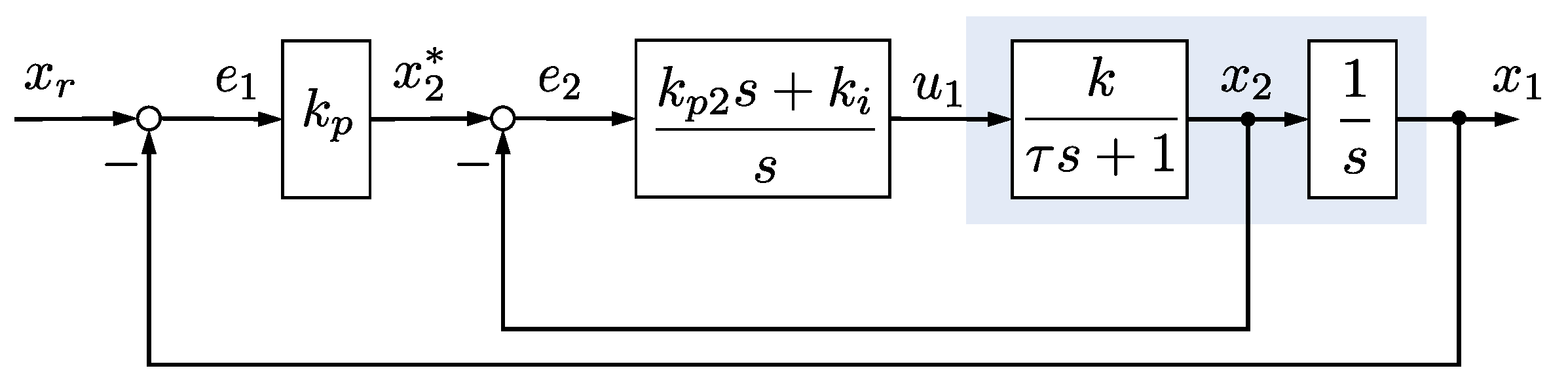
2.2. Cascade Controller Design and Performance

For the case of (3), the cascade controller is designed such that the outer-loop controller tracks a reference position signal $x_r$, while the inner-loop controller ensures that $x_2$ tracks a velocity reference signal $x_2^{\ast }$, as depicted in Figure 1. The cascade structure is constructed with a proportional (P) outer-loop controller and a proportional–integral (PI) inner-loop. The outer-loop controller is designed such that the tracking error $e_1\to 0$ at the rate $e^{-k_{p}t}$ for $k_p>0$, where $e_1=x_r-x_1$, i.e., $x_2^{\ast }=k_p{e}_1$. The outer-loop gain is, thus, obtained based on a desired time constant ${\tau }_1=k_p^{-1}$.

Remark 2.

In the context of this paper, the design parameter ${\tau }_1$ will serve as the transient performance criterion by which the transient response of the proposed controller will be evaluated. This parameter will be set based on a desired settling time of $T_s=3.91{\tau }_1$, corresponding to settling within $2\%$ of the reference value. The ability of the cascade structure to isolate the outer loop and independently control it as a first-order system is crucial, as in higher-order systems, such as an IMP-based closed-loop system, the time constant alone does not fully determine convergence time, as a result of oscillations and damping significantly influencing performance.

The inner-loop PI controller is designed to ensure that the tracking error $e_2\to 0$ through

$$u_1=k_{p2}{e}_2+k_i{\int }_0^t{e}_{2}d\tau \triangleq k_{p2}{e}_2+k_i\eta$$

(7)

where $e_2=x_2^{\ast }-x_2$. The gains $k_{p2}$ and $k_i$ are designed for the extended inner-loop system

$${\dot{\varphi }}_1=\left[\begin{array}{cc}-a& 0\\ -1& 0\end{array}\right] {\varphi }_1+\left[\begin{array}{c}b\\ 0\end{array}\right] u={\overline{A}}_1{\varphi }_1+{\overline{B}}_{1}u$$

(8)

where ${\varphi }_1={\left[\begin{array}{cc}{x}_2& \eta \end{array}\right]}^T$. As the pair $\left({\overline{A}}_1,{\overline{B}}_1\right)$ is controllable, the inner loop can be assigned arbitrary dynamics through (7) using the pole-placement method by selecting a location $\left[\begin{array}{cc}-{\lambda }_1& -{\lambda }_1\end{array}\right]$ for ${\lambda }_1>0$ on the real axis. The asymptotic stability and the zero steady-state error are guaranteed in both loops of the cascade control system as a result of setting $k_p>0$ and ${\lambda }_1>0$. To ensure that the outer-loop design criteria are maintained, the inner-loop dynamics is restricted as ${\lambda }_1\ge 3k_p$. The resulting cascade controller closed-loop system is constructed with the state vector ${\psi }_1={\left[\begin{array}{cc}{x}^T& \eta \end{array}\right]}^T$ as

$${\dot{\psi }}_1=\left[\begin{array}{ccc}0& 1& 0\\ -b{k}_p{k}_{p2}& -a-b{k}_{p2}& b{k}_i\\ -k_p& -1& 0\end{array}\right] {\psi }_1+\left[\begin{array}{c}0\\ b{k}_p{k}_{p2}\\ k_p\end{array}\right] x_r=A_1{\psi }_1+B_1{x}_r.$$

(9)

To demonstrate the advantage and shortcoming of the cascade controller, we consider the reference signal, measured in radians, as

$$x_r\left(t\right)=\left\{\begin{array}{cc}5,\hfill & \mathrm{for}0\mathrm{s}<t\le 5\mathrm{s}\hfill \\ 10,\hfill & \mathrm{for}5\mathrm{s}<t\le 10\mathrm{s}\hfill \\ 10sin{\omega }_{0}t,\hfill & \mathrm{for}10\mathrm{s}<t\le 20\mathrm{s}\hfill \\ 5,\hfill & \mathrm{for}20\mathrm{s}<t\le 25\mathrm{s}\hfill \end{array}\right.$$

(10)

with ${\omega }_0=2$ rad/s. The reference was tracked by assigning the cascade controller dynamics with ${\tau }_1=0.05{\zeta }_1$ for ${\zeta }_1\in [0.5,1.5]$. The nominal reference tracking performance of the controller (7), presented in Figure 2, demonstrates effective transient performance with fast convergence and no overshoot, provided that the dynamics is not too fast. However, the controller fails to achieve zero steady-state error for dynamic references, such as sinusoidal inputs. A limitation arises due to the inherent dynamics of the control structure, which does not account for time varying references. The model parameters used in the simulation of Figure 2 are detailed in Section 3. The next subsection explores how the sinusoidal reference tracking error observed in the case of the cascade subcontroller can be avoided through the used of an IMP-based subcontroller.

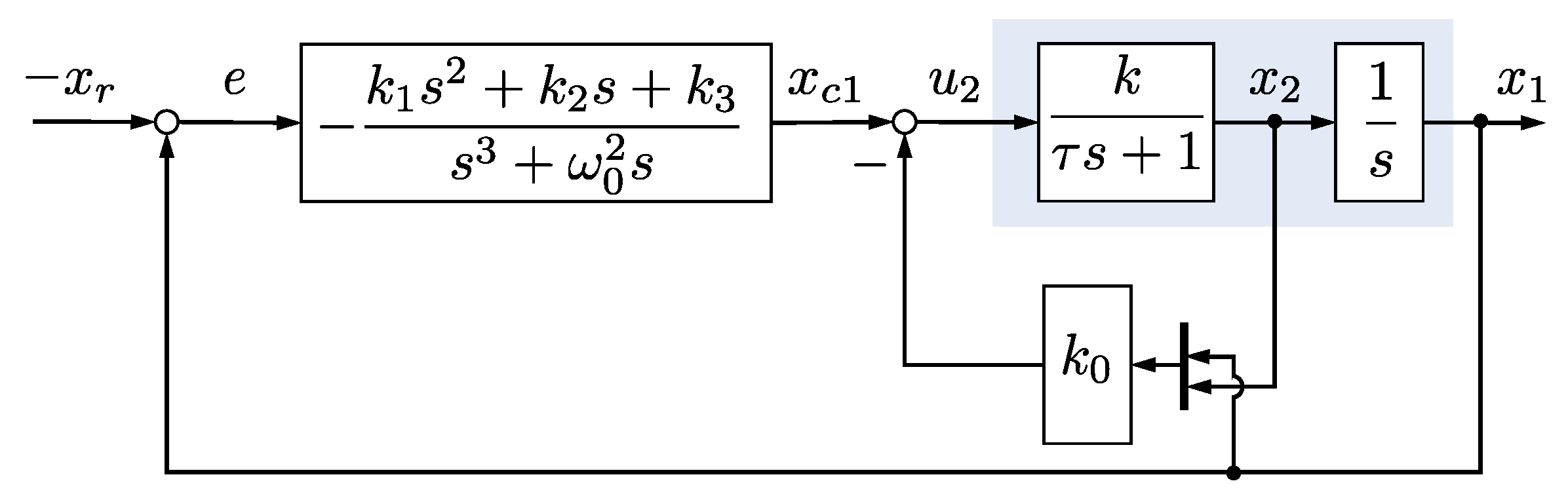
2.3. IMP-Based Controller Design and Performance

For the nominal system model (3), the IMP-based controller, shown in the closed-loop system of Figure 3, is designed based on the third-order differential equation ${\stackrel{⃛}{x}}_r+{\omega }_0^2{\dot{x}}_r=0$ satisfied by both (5) and (6). This equation enables the construction of an error-space dynamic system, with the error signal defined as $e=x_1-x_r=-e_1$. Taking the state vector as ${\varphi }_2={\left[\begin{array}{cccc}e& \dot{e}& \ddot{e}& {\xi }^T\end{array}\right]}^T$, the system dynamics can be represented in the error space as

$${\dot{\varphi }}_2=\left[\begin{array}{cccc}0& 1& 0& 0\\ 0& 0& 1& 0\\ -{\alpha }_3& -{\alpha }_2& -{\alpha }_1& C\\ 0& 0& 0& A\end{array}\right] {\varphi }_2+\left[\begin{array}{c}0\\ 0\\ 0\\ B\end{array}\right] \mu ={\overline{A}}_2{\varphi }_2+{\overline{B}}_2\mu$$

(11)

where $\xi \triangleq \stackrel{⃛}{x}+{\alpha }_1\ddot{x}+{\alpha }_2\dot{x}+{\alpha }_{3}x$ is defined as the error-space internal state variable, and $\mu \triangleq \stackrel{⃛}{u}+{\alpha }_1\ddot{u}+{\alpha }_2\dot{u}+{\alpha }_{3}u$ defined as the error space system input variable [3]. It is noted that ${\alpha }_1={\alpha }_3=0$ and ${\alpha }_2={\omega }_0^2$ following ${\stackrel{⃛}{x}}_r+{\omega }_0^2{\dot{x}}_r=0$.

Remark 3.

Based on the IMP method, ${\omega }_0$, which governs (5) and (6), is directly incorporated into the problem formulation as (11), allowing the control problem to be addressed within an error space. This ensures that the error approaches zero, even when the output follows a nondecaying command, such as a ramp signal, and maintains accuracy in the presence of parameter variations [3].

As the pair $\left({\overline{A}}_2,{\overline{B}}_2\right)$ is controllable, the error-space closed-loop system can be assigned arbitrary dynamics by setting the poles to a location ${\lambda }_2$ with the state feedback control law

$$\mu =-K{\varphi }_2=-\left[\begin{array}{cccc}{k}_3& k_2& k_1& k_0\end{array}\right] {\varphi }_2.$$

(12)

The system control input can be derived from the two definitions of the error-space system input $\mu$. Manipulating the terms of the two definitions and substituting the definition of the error-space system internal state $\xi$ provides

$${\displaystyle \frac{d^3}{d{t}^3}}\left(u+k_{0}x\right)=-{\alpha }_1{\displaystyle \frac{d^2}{d{t}^2}}\left(u+k_{0}x\right)-k_1{\displaystyle \frac{d^{2}e}{d{t}^2}}-{\alpha }_2{\displaystyle \frac{d}{dt}}\left(u+k_{0}x\right)-k_2{\displaystyle \frac{de}{dt}}-{\alpha }_3\left(u+k_{0}x\right)-k_{3}e.$$

(13)

Defining ${\dot{x}}_{c3}=-{\alpha }_3\left(u+k_{0}x\right)-k_{3}e$ and integrating (13) yields

$${\displaystyle \frac{d^2}{d{t}^2}}\left(u+k_{0}x\right)=-{\alpha }_1{\displaystyle \frac{d}{dt}}\left(u+k_{0}x\right)-k_1{\displaystyle \frac{de}{dt}}-{\alpha }_2\left(u+k_{0}x\right)-k_{2}e+x_{c3}.$$

(14)

Repeating the process by defining ${\dot{x}}_{c2}=-{\alpha }_2\left(u+k_{0}x\right)-k_{2}e+x_{c3}$, the equation can be rewritten as

$${\displaystyle \frac{d}{dt}}\left(u+k_{0}x\right)=-{\alpha }_1\left(u+k_{0}x\right)-k_{1}e+x_{c2}.$$

(15)

Finally, defining $x_{c1}=u+k_{0}x$ and the IMP controller state vector as $x_c={\left[\begin{array}{ccc}{x}_{c1}& x_{c2}& x_{c3}\end{array}\right]}^T$ allows the controller dynamic equation to be expressed using the state space equation

$${\dot{x}}_c=\left[\begin{array}{ccc}-{\alpha }_1& 1& 0\\ -{\alpha }_2& 0& 1\\ -{\alpha }_3& 0& 0\end{array}\right] x_c+\left[\begin{array}{c}-k_1\\ -k_2\\ -k_3\end{array}\right] e=A_c{x}_c+B_{c}e.$$

(16)

The output of the controller dynamics system is obtained as $x_{c1}=\left[\begin{array}{ccc}1& 0& 0\end{array}\right]x_c$. Alternatively, the output of the third-order IMP controller dynamic system can be obtained from the transfer function derived from (16) as

$${\displaystyle \frac{X_{c1}\left(s\right)}{E\left(s\right)}}=-{\displaystyle \frac{k_1{s}^2+k_{2}s+k_3}{s^3+{\alpha }_1{s}^2+{\alpha }_{2}s+{\alpha }_3}}.$$

(17)

Using the output of the IMP controller dynamic equation, the control input is constructed as

$$u_2=x_{c1}-k_{0}x$$

(18)

with $k_0=\left[\begin{array}{cc}{k}_{01}& k_{02}\end{array}\right]$. It is noted that the IMP control effort in (18) is represented as $u_2$ as it will be used as the second controller along with the first one (7) in the proposed hybrid structure framework. The closed-loop system resulting from the application of (18) to (3) is realized as

$${\dot{\psi }}_2=\left[\begin{array}{ccccc}0& 1& 0& 0& 0\\ -b{k}_{01}& -a-b{k}_{02}& b& 0& 0\\ -k_1& 0& -{\alpha }_1& 1& 0\\ -k_2& 0& -{\alpha }_2& 0& 1\\ -k_3& 0& -{\alpha }_3& 0& 0\end{array}\right] {\psi }_2+\left[\begin{array}{c}0\\ 0\\ k_1\\ k_2\\ k_3\end{array}\right] x_r=A_2{\psi }_2+B_2{x}_r$$

(19)

with the state vector ${\psi }_2={\left[\begin{array}{cc}{x}^T& x_c^T\end{array}\right]}^T$.

The nominal reference tracking performance of the IMP-based controller (18) is presented in Figure 4 by assigning ${\lambda }_2=\left[\begin{array}{ccccc}-25& -25& -25& -20& -30\end{array}\right] {\zeta }_2$, ${\zeta }_2\in [0.7,1.3]$. The tracking performance is characterized by zero tracking error for both constant and sinusoidal references. However, it is evident that the transient response exhibits significant overshoot. Reducing the gain ${\zeta }_2$ for the controller only decreases the convergence speed with both types of references without removing the transient overshoot.

While both controllers offer unique advantages, implementing either structure individually involves a trade-off between achieving a fast transient response and maintaining zero tracking error. Moreover, as shown through the simulations, adjusting the dynamics of either controller merely accentuates their inherent limitations without leading to a significant performance improvement. In the next section, an RL-based hybrid structure framework is formulated to integrate the unique advantages of the two control methods, without involving the limitations highlighted above, to construct a hybrid structure framework that can offer zero steady-state sinusoidal reference tracking error with fast transient-state convergence.

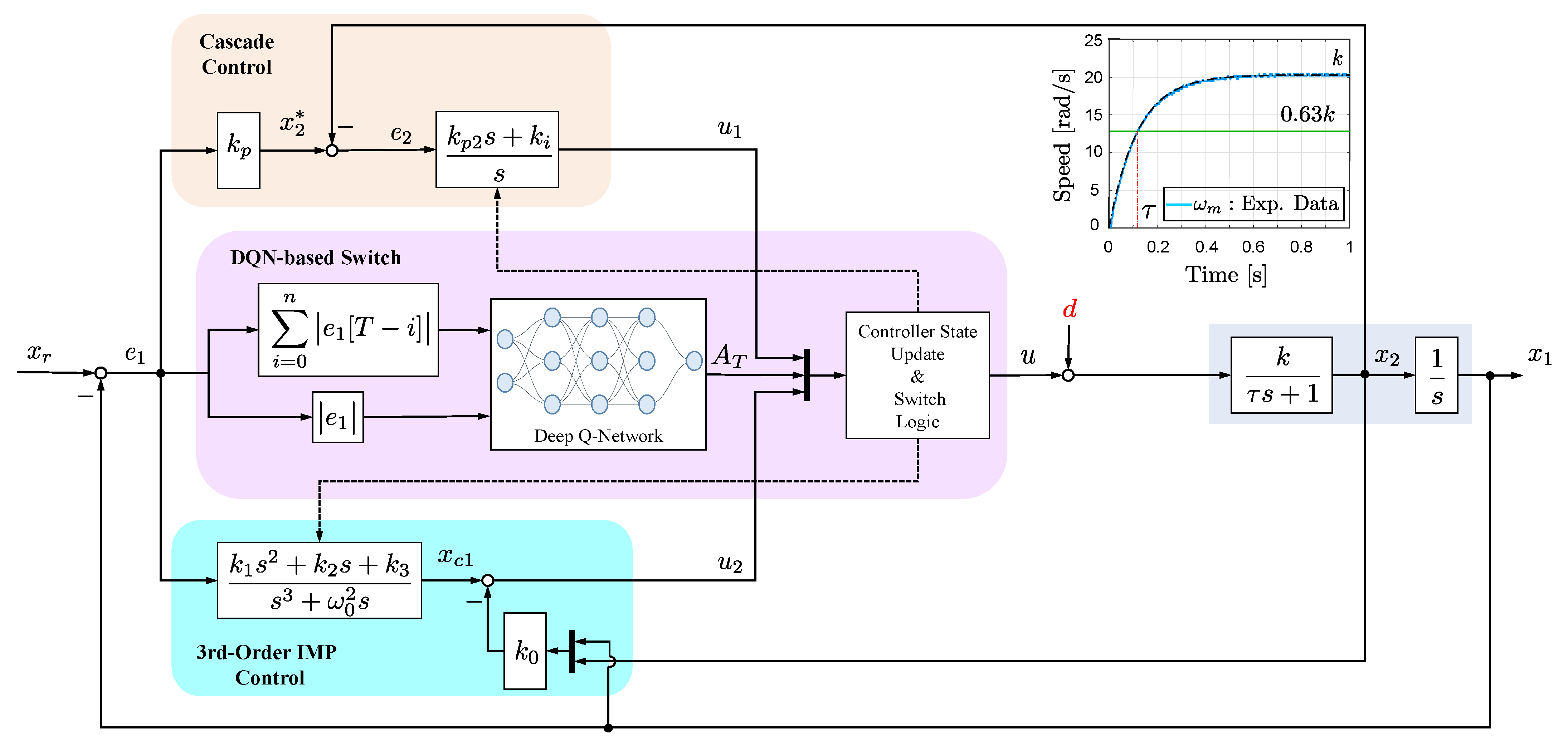
3. DQN-Based Hybrid Controller Design

3.1. Hybrid Structure Controller

As demonstrated in the previous section, ${\psi }_1$ offers a faster response and arguably superior transient stability due to its reduced number of dynamic components, while ${\psi }_2$ ensures zero tracking error for dynamic reference trajectories and offers enhanced robustness. These complementary characteristics suggest that by integrating the rapid response of ${\psi }_1$ with the robustness and precision of ${\psi }_2$, an enhanced closed-loop system can be achieved by a piecewise constant switching signal $\sigma$ that specifies the active subsystem at any time step T through the control law

$$u\left[T\right]=(1-\sigma \left[T\right])u_1\left[T\right]+\sigma \left[T\right]u_2\left[T\right],\sigma \in \{0,1\}$$

(20)

with $\sigma \left[T\right]=0$ to set $\psi \left[T\right]\leftarrow {\psi }_1\left[T\right]$, and $\sigma \left[T\right]=1$ for $\psi \left[T\right]\leftarrow {\psi }_2\left[T\right]$. To fully realize the control effort (20), a DQN model is used to generate the switching signal $\sigma$, enabling the dynamic selection of the comparatively optimal ${\psi }_p,p\in \{1,2\}$ based on real-time performance metrics. The closed-loop system of the proposed hybrid structure controller is depicted in Figure 5.

During training, RL-based control methods can raise safety concerns in real-world physical systems due to the potential for exploratory control actions to cause critical instability [32,39,40]. To mitigate these risks, the DQN model was trained offline on a closed-loop system designed for a DC motor, identified using the setup shown in Figure 6.

The experiment setup includes a commercial IG-32GM 09TYPE DC motor equipped with a 512PPR EE3020 optical encoder for high-resolution angular measurements. The encoder signals were calibrated before testing, and a sampling rate of 1 kHz was used for data acquisition to ensure accurate performance monitoring. Data acquisition and control implementation were carried out on an ARM Cortex-M3 ATSAM3X8E-based Arduino DUE board, utilizing its quadrature decoder and built-in low-pass filter for precise encoder signal processing. The DQN training involved discretizing both controllers using the Tustin method with a 1 ms sample period. Consequently, a 1 kHz sample rate is maintained throughout the training and validation processes presented in the paper. The setup was also used to validate the robustness of the proposed hybrid controller, discussed in Section 4.

Model identification was performed via an open-loop step response experiment, which provided the motor speed data shown in Figure 5. From the data, nominal plant parameters $\tau =0.1192$ and $k=20.2981$ of (2b) were identified (also used in the simulations of Figure 2 and Figure 4). For the training, the controller design parameters were set as ${\tau }_1=0.05$ and ${\lambda }_2=\left[\begin{array}{ccccc}-25,& -25,& -25,& -20,& -30\end{array}\right]$ to ensure satisfactory performance in their respective domains. The next subsection discusses the design of the controller dynamic system state update and switch logic.

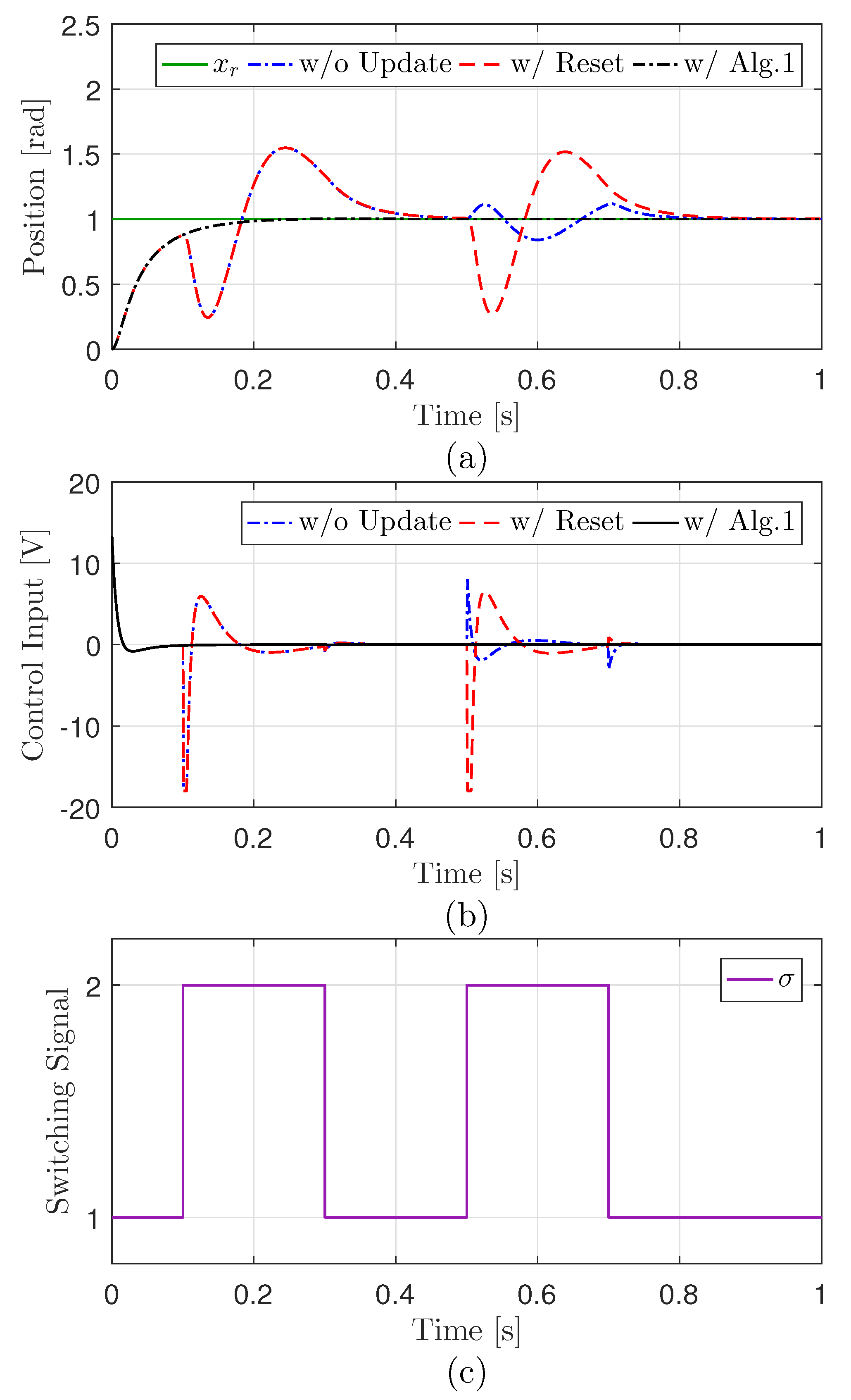
3.2. Controller State Update and Switch Logic

The transition between ${\psi }_1={\left[\begin{array}{cc}{x}^T& \eta \end{array}\right]}^T$ and ${\psi }_2={\left[\begin{array}{cc}{x}^T& x_c^T\end{array}\right]}^T$ needs to be smooth. During the transitions, the system model states in x remain continuous as (3) is in both closed-loop systems. However, the controller states $\eta$ and $x_c$ will have discontinuities when their respective subsystems are inactive. To maintain bumpless transfer, a discrete inner-state update logic is implemented (see Algorithm 1 below). The update logic is derived considering the case where the subsystems operate separately, as depicted in Figure 1 and Figure 3. In these nonswitched cases, at any given time step T, the discretized version of (7) generates $u_1\left[T\right]$ using $u_1[T-1]$ and $e_2[T-1]$, as described in

$$U_1\left(z\right)={\displaystyle \frac{m_1+m_2{z}^{-1}}{n_1+n_2{z}^{-1}}}{E}_2\left(z\right)$$

(21)

where $m_j$ and $n_j$ ($j=1,2$) are the coefficients of the numerator and denominator polynomials of the discretized PI controller, respectively. Similarly, for the IMP-based controller, the state $x_{c1}\left[T\right]$ is generated based on $x_{c1}[T-j]$ and $e_1[T-j](j=1,2,3)$ as expressed in

$$X_{c1}\left(z\right)={\displaystyle \frac{p_1+p_2{z}^{-1}+p_3{z}^{-2}+p_4{z}^{-3}}{q_1+q_2{z}^{-1}+q_3{z}^{-2}+q_4{z}^{-3}}}{E}_1\left(z\right)$$

(22)

where $p_j$ and $q_j$ ($j=1,\cdots ,4$) are the coefficients of the numerator and denominator polynomials of the discretized IMP-based controller, respectively. In these cases, the previous time step information used by (21) and (22) are directly correlated with the respective systems and require no alteration. However, for the case of the hybrid framework, when $\sigma \left[T\right]$ activates subcontroller i, the states of the inactive subcontroller $i^{\prime }$, which will potentially be utilized in the time step $T+1$, must be updated using the outputs of the plant model and the active subcontroller i in the time step T, as outlined in Algorithm 1.

Algorithm 1 Controller state update and switch logic

1: if  $A_T=0$  then 2:    $u\left[T\right]=u_1\left[T\right]$ 3:    for $j=1$ to 3 do 4:      $x_{c1}[T-j]\leftarrow u[T-(j-1)]+k_0\left[\begin{array}{c}{x}_1[T-j+1]\\ x_2[T-j+1]\end{array}\right]$ 5:    end for 6: else if $A_T=1$ then 7:    $u\left[T\right]=u_2\left[T\right]$ 8:    $u[T-1]\leftarrow u\left[T\right]$ 9:    $e_2[T-1]\leftarrow k_p{e}_1\left[T\right]-x_2\left[T\right]$ 10: end if

The effectiveness of the update logic is shown in Figure 7 through a simulation where the hybrid controller tracks a reference $x_r=1$ rad with an arbitrary switching signal $\sigma$. The plot compares three cases: subsystem switching without update, with state reset, and with the update logic of Algorithm 1. When the controller states are reset or not updated, switching to ${\psi }_2$ (when $\sigma \left[T\right]\to 2$) causes significant perturbations in both control input and system output. In contrast, Algorithm 1 ensures smooth subsystem transfers at all the switching instances. The next subsection presents the RL model training process used in the paper.

3.3. Reinforcement-Learning-Based Switching Function

The DQN model is trained to provide a nonlinear mapping from $e_1$ to $\sigma$. Thus, within the RL framework, the optimal switching signal that determines the hybrid structure control input for a given state s is derived from the optimal policy ${\pi }^{\ast }$ as $\sigma ={\pi }^{\ast }\left(s\right)={argmax}_{a\in A}{\mathcal{Q}}^{\ast }(s,a)$. To learn this policy, the MDP (Markov decision process) components are formalized as follows:

• Environment: The environment was modeled as the identified system (3) tracking the reference signal (10).
• State: The state at time step T was constructed as

  $$S_T={\left[\begin{array}{cc}{\displaystyle {\nu }_1\sum _{i=0}^n\left|e_1[T-i]\right|,}& {\nu }_2\left|e_1\left[T\right]\right|\end{array}\right]}^T$$

  (23)

  with $n=25$ and ${\nu }_1={\nu }_2=1$ taken as additional tuning parameters. The state $S_T$ was constructed using only $e_1$, as this parameter highlighted key performance disparities between the two subcontrollers.
• Action: The action $A_T\in A\left(s\right)$ available at any time step is the discrete control effort of either (7) or (18), allowing the action space to be formulated as the binary space $A\left(s\right)=\{0,1\}$ where 0 and 1 represent the saturated $u_1$ and $u_2$, respectively, with saturation at $\pm 18.0$ V. Hence, in the context of the DQN-based controller, $A_T=\sigma$ at any given time step T.
• Reward: As the design objective of the hybrid structure controller is to minimize $e_1$, the reward function is constructed as the linearly scaled value of the current time step squared error as $R_T=-\beta {\left(e_1\left[T\right]\right)}^2$. To ensure $|e_1|\to 0$, we set $\beta \gg 1$, with $\beta ={10}^3$. Constructing $R_T$ solely based on $e_1$ offers a clear objective that facilitates straightforward training.

To preserve the low computational resource requirement of the subcontrollers, the DQN was designed with a minimal three-layer architecture, featuring leaky ReLU, sigmoid, and linear output layers, each with three nodes, totaling 29 learned parameters. While such compact design is ideal for resource-constrained scenarios, a larger model could be employed in resource-abundant environments to capture more complex MDP features. Although methods employing neural networks typically impose a higher computational burden compared to conventional schemes such as PID control, the compact architecture of the DQN model and the low-order dynamics of the subcontrollers ensure that the proposed hybrid controller introduces only minimal computational overhead. This makes it well suited for deployment on embedded hardware. The DQN was trained using PyTorch (version 2.1.0) with the algorithm outlined in Algorithm 2 and the hyperparameters listed in

Table 1. DQN training hyperparameters.

Hyperparameter	Value	Hyperparameter	Value
$\epsilon$	0.01	Learning Rate ($\alpha$)	${10}^{-5}$
${\epsilon }_{\mathrm{decay}}$	0.995	Episodes	200
Discount Factor ($\gamma$)	0.4	Soft Update Parameter	0.05
Replay Memory Size	$5\times {10}^4$	Batch Size	${10}^3$
Optimizer	Adam	Loss Function	L1 Loss

.

Algorithm 2 DQN training for hybrid controller

1: Initialize discretized plant and controller structure (20) 2: Initialize policy network $\mathcal{Q}$ and target network $\widehat{\mathcal{Q}}$ 3: Copy policy network weights to target network 4: Initialize replay buffer $\mathcal{D}$ to specified memory size 5: for each episode in Episodes do 6:    Initialize state $S_T$ to $S_0$ 7:    for each time step T do 8:      Compute [$u_1$, $u_2$] and select $\epsilon$-greedy $A_T\in A\left(s\right)$ 9:      Apply Algorithm 1 10:      Pass u to discrete plant model and receive [$R_T$, $S_{T+1}$] 11:      Store transition $(S_T,A_T,R_T,S_{T+1})$ in $\mathcal{D}$ 12:      Sample random mini-batch of transitions from $\mathcal{D}$ 13:      Compute target Q-value 14:      Perform gradient descent on the loss function 15:      Soft update target network 16:    end for 17: end for

Remark 4.

The DQN training followed the standard RL framework [33] utilizing a soft target update mechanism for the target network [41], with enhancements made to incorporate the elements of the proposed hybrid controller, i.e., the initialization of the discretized dynamic systems and Algorithm 1.

3.4. Discussion on Stability

The closed-loop system resulting from the application of the hybrid control input (20) is written as

$${\dot{\psi }}_p=A_p{\psi }_p+B_p{x}_r,p\in \{1,2\}.$$

(24)

The DQN model generates a piecewise constant switching signal $\sigma$ that specifies the active subsystem $p\in \{1,2\}$ at any time step T. As the pairs $({\overline{A}}_p,{\overline{B}}_p)$ in (8) and (11) are controllable, the individual closed-loop systems can be assigned arbitrary dynamics in (9) and (19). This guarantees that $A_p,p\in \{1,2\}$ in (24) is Hurwitz. Additionally, the switching signal $\sigma :[0,\infty )$ in (20) is sufficiently regular with finite number of discontinuities or switching times. The switches of $\sigma$ occurring at switching times $t_1,t_2,\cdots$ are restricted to satisfy the inequality $t_{i+1}-t_i\ge {\tau }_d$, where the dwelling time ${\tau }_d>0$ represents the duration any given subsystem remains active [12]. This restriction is imposed to allow the transient effects to dissipate after each switch. For the case of (24), a sufficiently large ${\tau }_d=1$ ms was selected. It is established in [12] that when all linear systems in the family (24) are asymptotically stable, the switched linear system governed by $\sigma$ is asymptotically stable provided that the dwell time ${\tau }_d$ is sufficiently large.

While the conditions for asymptotic stability of the closed-loop system under the proposed DQN-based hybrid control scheme are briefly stated, a detailed derivation and rigorous stability analysis are beyond the scope of this paper. Readers interested in an in-depth exploration of the stability conditions are encouraged to refer to the comprehensive treatment provided in [12]. This paper primarily focuses on developing and validating the control scheme, emphasizing reference tracking and nominal performance recovery over detailed stability analysis [42,43]. The next subsection presents the DQN model training outcome and the resulting performance enhancement obtained from the hybrid structure controller.

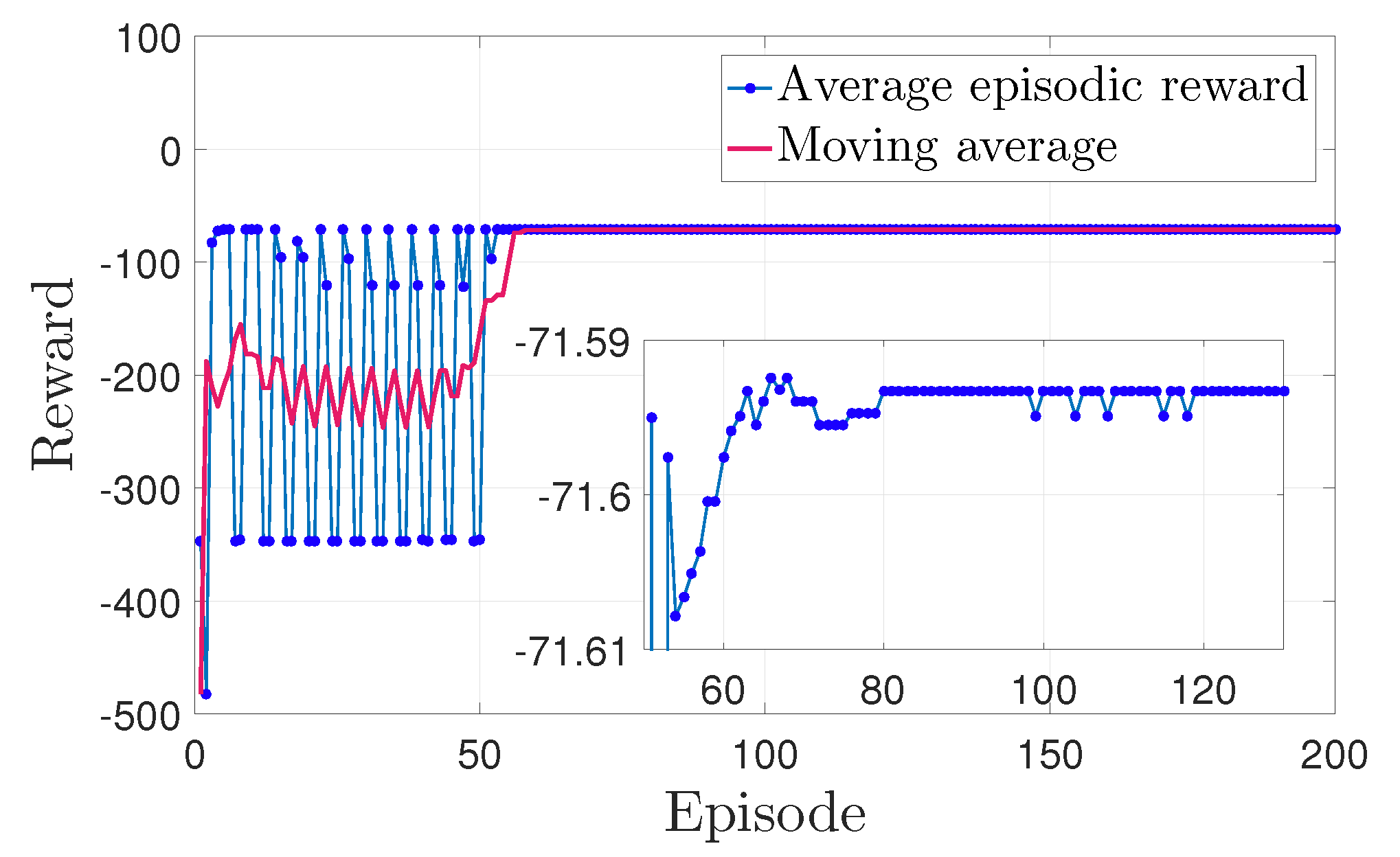
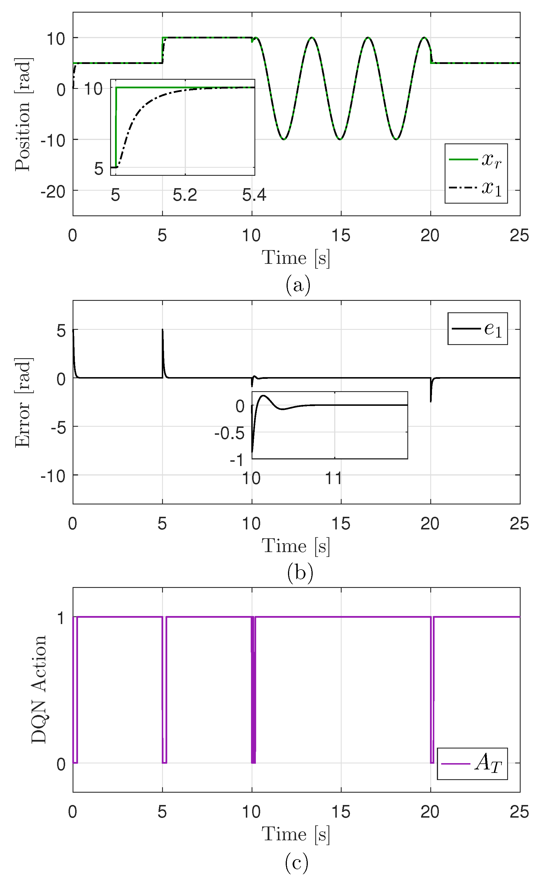
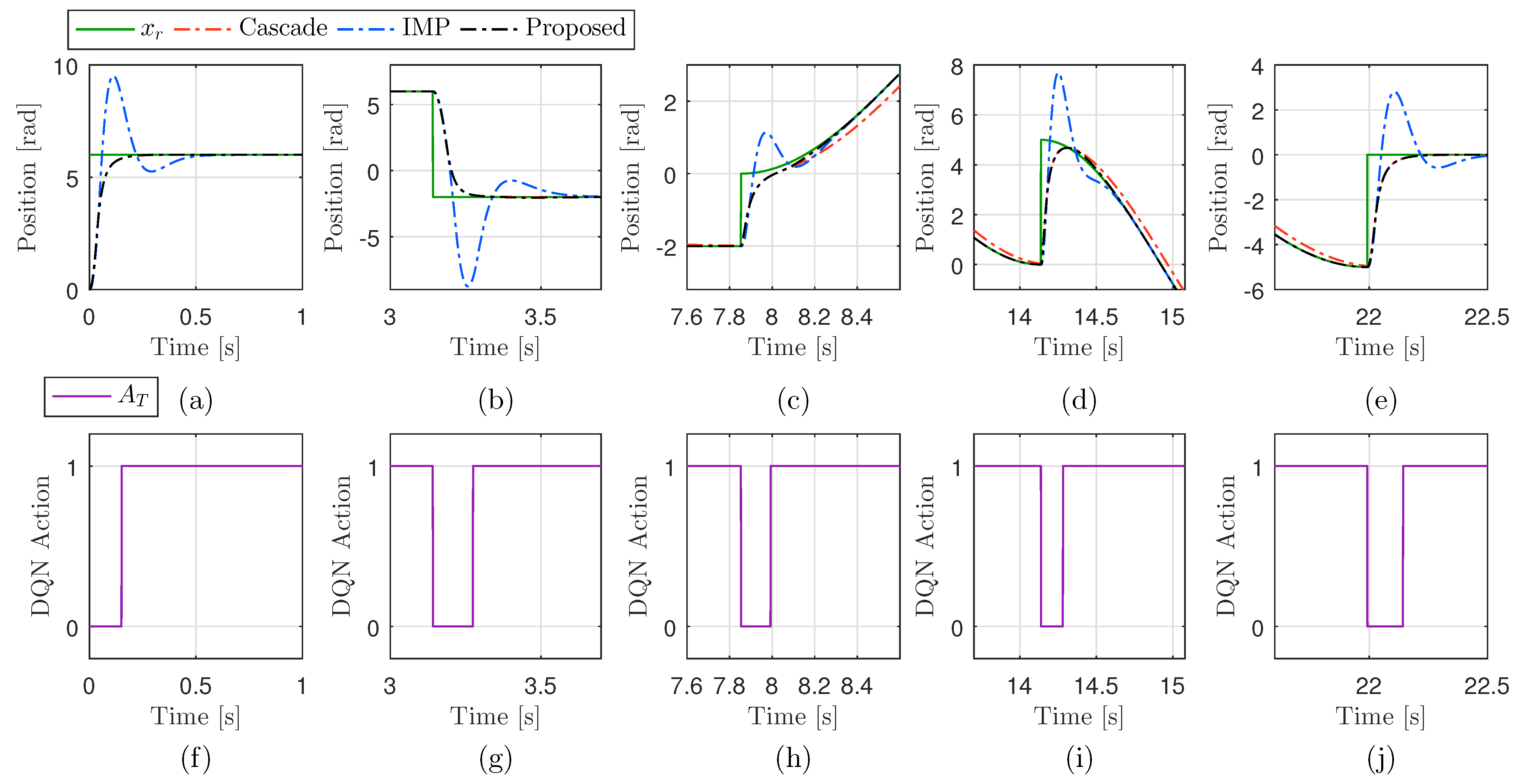
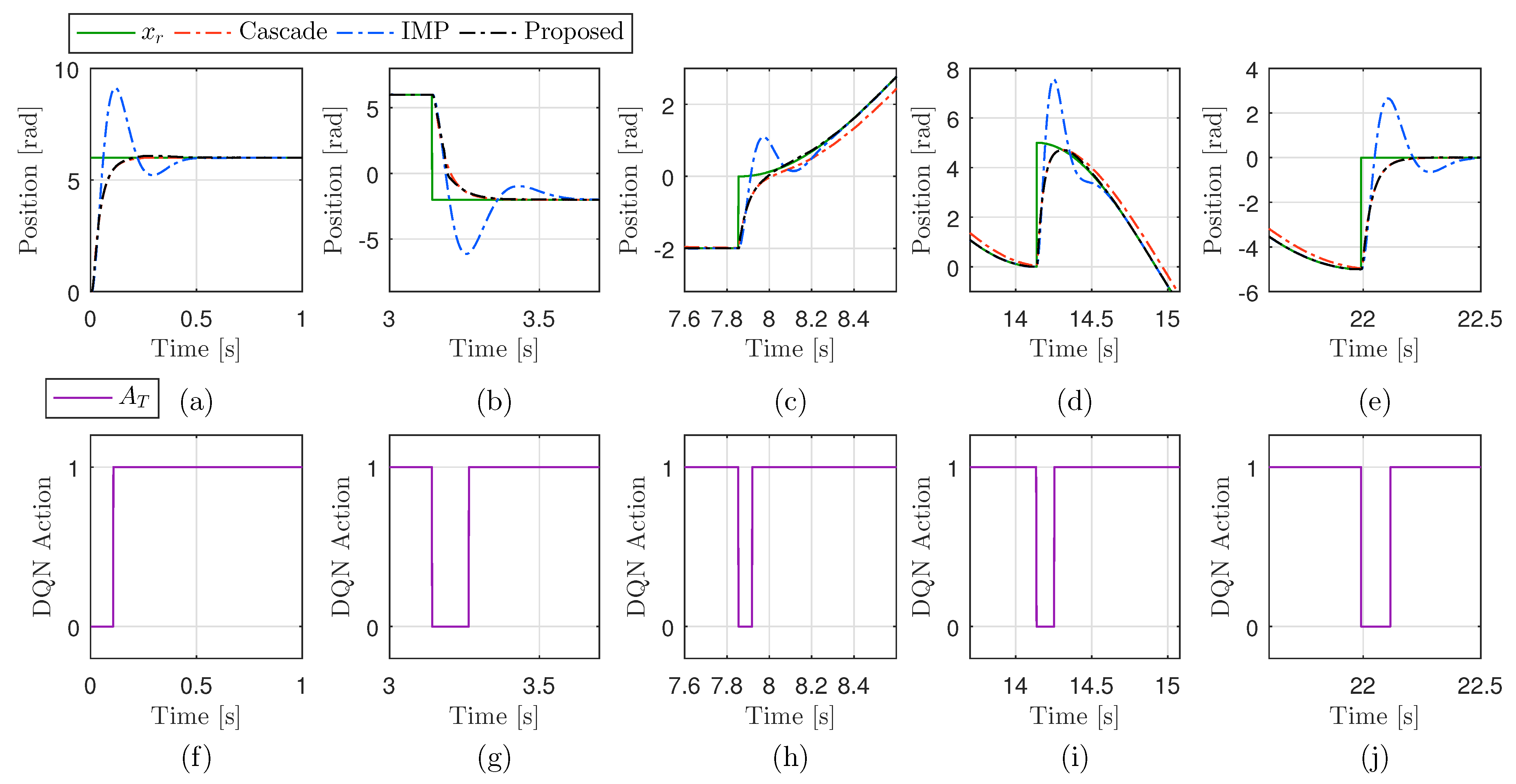
3.5. DQN Training Result and Hybrid Controller Nominal Performance

The DQN training reward history is presented in Figure 8 with a 10-episode moving average. Early episodes display significant fluctuations as the agent explores the environment. In particular, fluctuations with similar amplitudes occurred, indicating episodes where the agent employed one subcontroller for the entire episode exclusively, with the lower bound corresponding to exclusively cascade subcontroller episodes and the higher bounds corresponding to exclusively IMP subcontroller episodes. Over time, an upward trend stabilizes around Episode 80, indicating that the model has found an optimal policy and is consistently receiving high rewards. The tracking performance of the proposed hybrid controller with the trained DQN is shown in Figure 9a,b. From the actions taken by the DQN model after the training, shown in Figure 9c, it can be seen that the model employed the IMP-based controller ($A_T=1$) for both the constant and sinusoidal segments of (10), switching to the cascade controller ($A_T=0$) during transient states. This strategy achieved zero steady-state tracking error without transient overshoot, outperforming both subcontrollers (see Figure 2 and Figure 4).

It should be noted that the rapid switches in Figure 9c represent controlled DQN decisions to optimize transient and steady-state performance and should not be regarded as the peaking phenomenon discussed in [38,44], typically characterized by uncontrolled, high-magnitude oscillations in control effort. It can be noticed that the actual control effort, presented below in Figure 10, along with the DQN action remains smooth and unsaturated.

The design procedure of the proposed DQN-based hybrid structure controller is visually represented through a flowchart in Figure 11. The performance validation of the proposed controller presented through both comparative simulations and experiment is discussed in the next section.

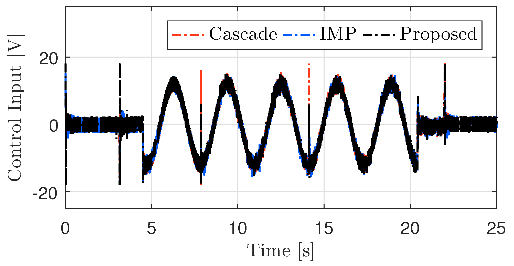
4. Robust Performance Test

Although outperforming the individual subcontrollers on the reference used for DQN training is promising, a more meaningful outcome would be demonstrating improved performance on a different reference not encountered during training. To evaluate this, a new reference trajectory, measured in radians, was constructed as follows:

$$x_r\left(t\right)=\left\{\begin{array}{cc}6,\hfill & \mathrm{for}0\mathrm{s}<t\le \pi \mathrm{s}\hfill \\ -2,\hfill & \mathrm{for}\pi \mathrm{s}<t\le 2.5\pi \mathrm{s}\hfill \\ 3sin(2t+0.5\pi )+3,\hfill & \mathrm{for}2.5\pi \mathrm{s}<t\le 4.5\pi \mathrm{s}\hfill \\ 5sin(2t-0.5\pi )\hfill & \mathrm{for}4.5\pi \mathrm{s}<t\le 7\pi \mathrm{s}\hfill \\ 0,\hfill & \mathrm{for}7\pi \mathrm{s}<t\le 25\mathrm{s}.\hfill \end{array}\right.$$

(25)

For robustness validation, an input channel external sinusoidal disturbance was taken as

$$d\left(t\right)=12sin(2t+1.5\pi )\mathrm{for}4.5\mathrm{s}<t\le 6.5\pi \mathrm{s}$$

(26)

along with the model parameter variations summarized in

Table 2. Model parameter uncertainties considered in the simulation.

Parameter	Nominal Value	Uncertain Value	Physical Representation
k	20.2981	25.3726	${\displaystyle \frac{K_t}{B_m{R}_a+K_t{K}_b}}$
$\tau$	0.1192	0.0953	${\displaystyle \frac{J_m{R}_a}{B_m{R}_a+K_t{K}_b}}$

, taken considering a $25\%$ increase in k and a $20\%$ reduction in $\tau$ in the nominal (3).

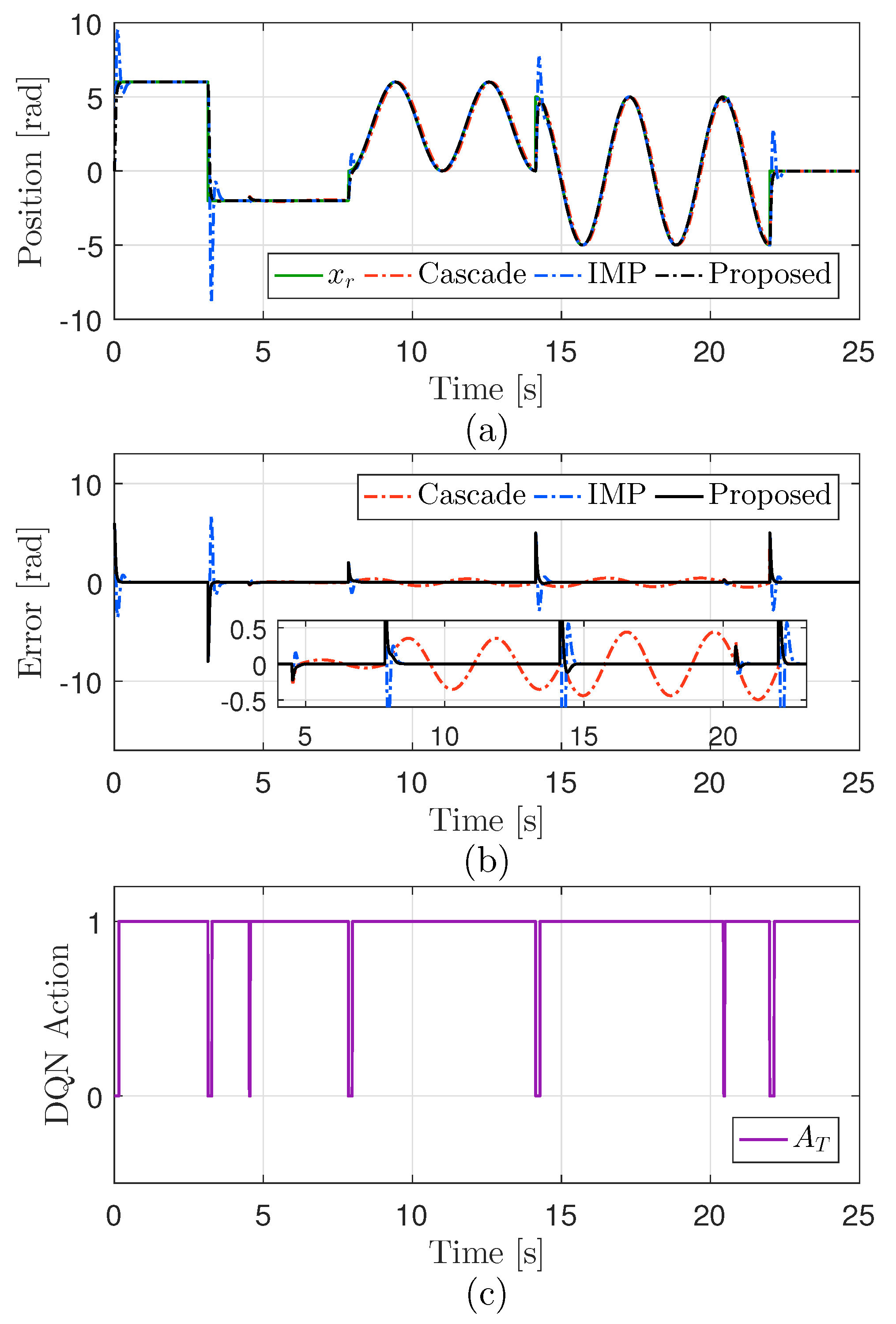
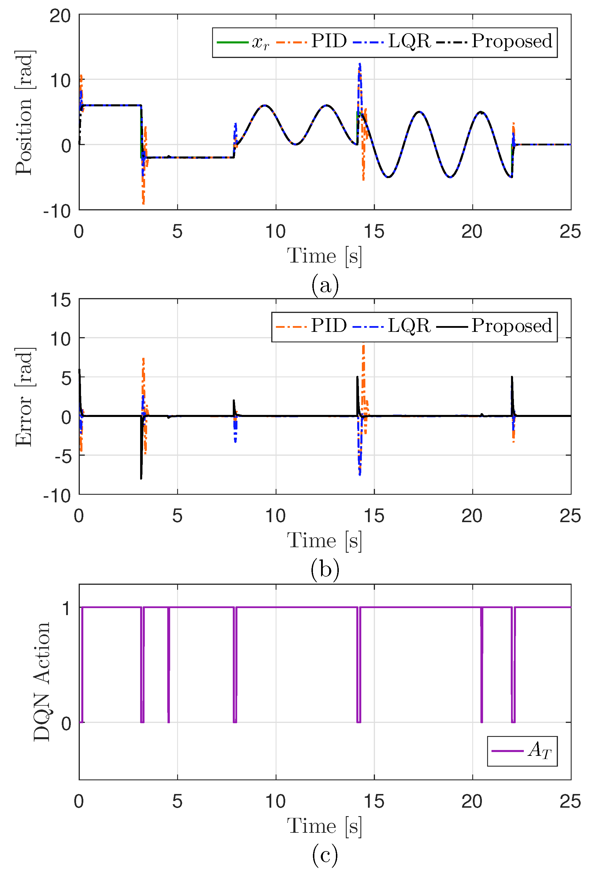
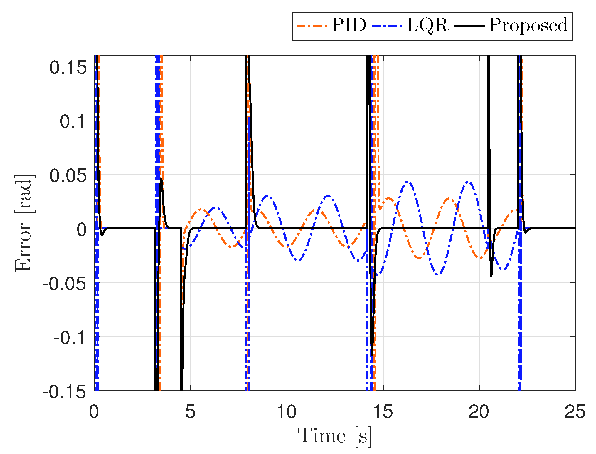
4.1. Performance Validation in Simulations

The simulation result, presented in Figure 12, shows a policy that aligns with the training result whereby the DQN employed the IMP-based structure ($A_T\to 1$) for tracking the constant and sinusoidal segments of (25), switching to the cascade structure ($A_T\to 0$) only during transients and disturbance instances, confirming that the proposed scheme can effectively offer enhanced performance on unknown reference signals. Moreover, the proposed controller avoids the tracking errors of the cascade structure and achieves zero steady-state error while tracking the sinusoidal reference under the sinusoidal disturbance owing to the action of the DQN model (see Figure 12b).

Each transient state, shown in Figure 13, reveals limitations of the IMP-based structure where overshoots occur. The proposed DQN-based hybrid scheme, complemented by the update logic in Algorithm 1, avoids these overshoots by transitioning to the next segment of the reference through the cascade structure and reverting to the IMP-based structure in the steady states to leverage its zero tracking error performance. Notably, at the transition between the two sinusoidal segments (Figure 13d), despite the inability of the cascade structure to achieve zero steady-state error for sinusoidal signals, it was briefly engaged by the DQN to prevent the transient overshoot.

The enhanced nominal performance recovery of the controller is demonstrated in Figure 14. Note that Figure 14a presents the tracking error comparison at the moment the disturbance signal (26) was introduced to the system, while Figure 14b depicts the moment the signal was removed. The demonstrated ability of the DQN model to enhance nominal performance recovery is an extension of the transient performance improvement, as uncertainties were not considered during training. Individually, both subcontrollers experience significant perturbations due to (26), presented in Figure 15a, along with the control effort comparison in Figure 15b. In contrast, the proposed scheme effectively minimizes perturbations by momentarily switching to the cascade structure. Thus, even while tracking a sinusoidal reference in the presence of a sinusoidal disturbance, the DQN engages the cascade structure to enhance nominal performance recovery. Moreover, the DQN adapts its strategy by assigning longer steps to the cascade structure during transients (Figure 13) compared to disturbance instances (Figure 14). To facilitate nominal performance recovery in the simulation, (23) was modified, taking $n=15$.

To further highlight the advantages of the proposed RL-based hybrid control scheme, additional comparative simulations were conducted in the same simulation environment discussed above, using two existing controllers: a PID controller and an LQR controller. The PID control input was formulated as

$$u_{PID}=k_{p2}\left(x_r-x_1\right)-k_d{x}_2+k_{i2}{\eta }_1$$

(27)

where ${\displaystyle {\eta }_1={\int }_0^t\left(x_r-x_1\right)d\tau }$. The PID gain matrix was determined by assigning the eigenvalues of the resulting closed-loop system to the locations ${\lambda }_{PID}=\left[\begin{array}{ccc}-40& -65& -90\end{array}\right]$. Similarly, the LQR controller was formulated as

$$u_{LQR}=k_{q1}\left(x_r-x_1\right)-k_{q2}{x}_2.$$

(28)

The LQR gains were obtained by minimizing the cost function ${\displaystyle J={\int }_0^{\infty }\left(x^{T}Qx+u^{T}Ru\right)dt}$, where the weighting matrices were set to $Q=q\left(C^{T}C\right);q={10}^5$ and $R=0.25$. The reference tracking performance from the simulation is shown in Figure 16. Below, Figure 17 is presented for a clearer view of the steady-state error comparison between the proposed scheme and the conventional controllers, with a magnified view of the tracking error comparison provided in Figure 17. Both the PID and LQR design parameters were iteratively tuned to limit the absolute value of the tracking error to less than 0.05 rad, as can be seen in Figure 17. The simulation results revealed that, while it is possible to employ fast dynamics to reduce the tracking error of the PID and LQR controllers within ±0.05 rad, a value that remains larger than the error achieved by the proposed hybrid method, the transient-state performance was adversely impacted as a consequence. This degradation is also evident in the saturated transient-state control efforts from the PID and LQR controllers, presented in Figure 18. Conversely, adjusting the control parameters to prioritize transient-state performance would inevitably further compromise the reference tracking accuracy. By assigning specific individual control structures to address different performance aspects and seamlessly integrating them through the proposed RL-based hybrid structure framework, these challenges can be effectively mitigated.

To further demonstrate the effectiveness of the proposed controller, the transient-state performance comparison with the individual subcontrollers (cascade and IMP), as well as the additional controllers (PID and LQR), is presented in tabular form. Specifically,

Table 3. Convergence time comparison with subcontrollers and conventional controllers in simulations.

Transient	Cascade Convergence [s]	IMP Convergence [s]	PID Convergence [s]	LQR Convergence [s]	Proposed Convergence [s]
1	0.17	0.46	0.25	0.17	0.17
2	0.13	0.44	0.37	0.20	0.13
3	Does Not Converge	0.47	Does Not Converge	Does Not Converge	0.38
4	Does Not Converge	0.47	Does Not Converge	Does Not Converge	0.32
5	0.17	0.47	0.21	0.13	0.18
Average	-	0.46	-	-	0.23

provides the convergence time for each controller, taken as the time required to converge within $\pm 2\%$ of the next reference signal segment, while

Table 4. Transient overshoot comparison with subcontrollers and conventional controllers in simulations.

Transient	Cascade Overshoot [%]	IMP Overshoot [%]	PID Overshoot [%]	LQR Overshoot [%]	Proposed Overshoot [%]
1	0	58.63	77.81	36.63	0.11
2	0	84.53	92.49	35.39	0.57
3	Does Not Converge	56.52	Does Not Converge	Does Not Converge	0
4	Does Not Converge	53.81	Does Not Converge	Does Not Converge	2.34
5	0	56.27	67.21	37.98	0.082
Average	-	61.95	-	-	0.62

presents the corresponding maximum percentage overshoots. In these tables, the five transient states correspond to transitions between consecutive segments of (25), presented in Figure 13. The data in the tables further highlight the key observation that when tracking a reference signal that includes both constant and sinusoidal segments, single-structure controllers, such as PID and LQR, fail to deliver effective transient-state performance. This limitation arises from the need to balance performance across both types of references, which compromises their overall effectiveness. While the cascade controller demonstrates strong transient-state performance, its inability to adapt to the dynamic reference signal renders it ineffective for sinusoidal tracking. The IMP controller, on the other hand, successfully tracks each segment of the reference signal with minimal tracking error, as presented in

Table 5. Average steady-state error comparison in simulation.

Reference Type	Cascade Avg. Err. [rad]	IMP Avg. Err. [rad]	PID Avg. Err. [rad]	LQR Avg. Err. [rad]	Proposed Avg. Err. [rad]
Constant (1 s $<t<$ 2 s)	$1.009\times {10}^{-9}$	$1.302\times {10}^{-6}$	$1.747\times {10}^{-15}$	$1.007\times {10}^{-17}$	$6.753\times {10}^{-8}$
Sinusoidal (9 s $<t<$ 12 s)	$2.216\times {10}^{-1}$	$6.561\times {10}^{-8}$	$1.113\times {10}^{-2}$	$1.852\times {10}^{-2}$	$3.665\times {10}^{-8}$

. From the steady-state error comparison presented in the table, it can be seen that while each controller offers a small tracking error when tracking the constant reference signal, only the IMP and proposed hybrid controller were able to maintain this performance for the case of a sinusoidal reference. On the other hand, Table 3 and Table 4 show that the IMP controller exhibited significantly large convergence time and overshoot, as discussed in detail in Section 2. By leveraging the DQN model to govern transitions between the cascade and IMP subcontrollers, the proposed hybrid structure controller offered the fastest convergence with both constant and sinusoidal reference signals (see Table 3), smallest overshoot (see Table 4), and maintained minimal steady-state reference tracking error throughout (see Table 5). It successfully tracks each segment of the reference signal while minimizing both overshoot and convergence time. This performance advantage underscores the hybrid structure controller’s ability to seamlessly balance transient-state and steady-state objectives. The next subsection presents the experimental validation results and associated discussion.

4.2. Performance Validation in Experiments

The practicality of the proposed scheme was validated through comparative experiments conducted using the setup in Figure 6. The experimental environment is illustrated in Section 3.1. As discrepancies between a simulation and an experiment caused by factors including unmodeled dynamics and parameter variations are unavoidable [39], the DQN input parameters were recalibrated by taking $n=8,{\nu }_1=1.55$, and ${\nu }_2=1.05$ in (23) to overcome these discrepancies. Note that ${\nu }_1$ is increased in $S_T$ as it weights the cumulative error over the previous time steps.

The resulting tracking performance obtained from the experiments, presented in Figure 19, closely mirrors the simulation results. The DQN effectively governed the hybrid controller to utilize the IMP-based structure for tracking the constant and sinusoidal segments of the reference, switching to the cascade structure only during transients (Figure 20) and disturbance instances (Figure 21).

To further analyze the experiment results, the performance enhancements achieved by the proposed controller are quantitatively presented in

Table 6. Convergence time comparison with subcontrollers in experiment.

Transient	Cascade Convergence [s]	IMP Convergence [s]	Proposed Convergence [s]
1	0.18	0.44	0.17
2	0.17	0.43	0.18
3	Does Not Converge	0.43	0.32
4	Does Not Converge	0.44	0.28
5	0.17	0.43	0.18
Average	–	0.43	0.22

,

Table 7. Transient overshoot comparison with subcontrollers in the experiment.

Transient	Cascade Overshoot [%]	IMP Overshoot [%]	Proposed Overshoot [%]
1	0.16	51.89	1.49
2	0.12	51.62	0.12
3	Does Not Converge	54.41	2.53
4	Does Not Converge	53.60	2.21
5	0.19	52.95	0.19
Average	–	52.91	1.31

and

Table 8. Average steady-state error comparison in the experiment.

Reference Type	Cascade Avg. Err. [rad]	IMP Avg. Err. [rad]	Proposed Avg. Err. [rad]
Constant (1 s $<t<$ 2 s)	$5.138\times {10}^{-4}$	$1.826\times {10}^{-3}$	$8.943\times {10}^{-4}$
Sinusoidal (9 s $<t<$ 12 s)	$2.123\times {10}^{-1}$	$3.233\times {10}^{-3}$	$3.395\times {10}^{-3}$

. Similar to the simulation results, Table 6 presents the time taken by each controller to converge within $\pm 2\%$ of the tracking error value at each of the five transient states of (25). Recalling the transient-state performance criteria set in Remark 2, and following the selection of ${\tau }_1=0.05$, the desired settling time of the system is approximately 0.2 s. Hence, from the average convergence time presented in Table 6, it can be seen that the proposed controller, which yielded 0.23 s, offers the closest value. Despite the ability of the cascade control structure to offer a relatively better transient-state performance, its inability to converge with the sinusoidal reference segments ultimately makes it unsuitable for such reference signals. Furthermore, it is noted that the deviation recorded from the actual target convergence time is owing to the model-order reduction in (2).

Similarly, Table 7 compares the percentage overshoot recorded from three controllers in the experiment. From the table it can be seen that while the IMP controller produced an average overshoot of approximately $52.91\%$, the proposed controller was able to reduce this figure to approximately $1.31\%$. This significant reduction in transient overshoot was achieved as a result of the capacity of the hybrid controller to momentarily switch into the cascade controller mode during each transient state, as shown in Figure 20. The effect of using the cascade control structure during transients was also extended to the nominal performance recovery performance of the proposed hybrid controller, as shown in Figure 21.

Consequently, the proposed controller maintained minimal steady-state tracking error for both reference types (see Table 8), complemented by significantly reduced overshoot and enhanced nominal performance recovery. A key distinction between the experiment and simulation is the shorter maintaining steps of the cascade structure in the experiment, underscoring the adaptive nature of the DQN-based scheme. The control effort data gathered during the experiments, depicted in Figure 22, also show that no control effort saturation occurred during the controller transfer in the proposed hybrid framework.

Regarding the impact of uncertainties on the performance of the proposed method, the performance validations conducted, considering parameter uncertainties and external disturbance signals, indicate that the proposed RL-based hybrid controller addresses these challenges effectively. As a robust control method, the IMP controller inherently handles uncertainties without requiring additional compensation, while the proposed hybrid structure, leveraging the learned policy, minimizes convergence time during transient states under uncertainty (Figure 13) and improves nominal performance recovery (Figure 21). Furthermore, the simulation results presented in Section 4.1 considered parameter variations. Although the proposed controller and conventional controllers considered in the simulations were able to handle the uncertainties considered in the simulations, for scenarios involving more severe uncertainties, such as parameter variations larger than those listed in Table 2 or external disturbance signals with different characteristics to (26), the performance of the controller can be further enhanced by measures including training a larger DQN model or incorporating a DOBC with moderately faster dynamics [36,37,45,46,47].

5. Conclusions

An RL-based hybrid control scheme was proposed to address the common trade-off in IMP controllers between achieving zero steady-state tracking error and fast transient response. The proposed scheme integrates a cascade and an IMP-based controller through a DQN-based switching and state update logic, to isolate their respective advantages and synthesize them into a hybrid framework. The DQN model was trained offline on the nominal closed-loop system. Performance validation, conducted through comparative simulations and experimental tests on a DC motor position control system, confirmed that the proposed scheme effectively integrated the fast transient response of the cascade structure with the precision and robustness of the IMP-based scheme, mitigating the limitations of single-structure implementation. To validate the robustness and adaptability of the proposed scheme, the performance validation was carried out using reference signal and uncertainties, including both model parameter variations and external disturbances, which were not considered during the DQN model training. The proposed controller achieved performance enhancement in key metrics, including faster convergence to the reference with reduced transient overshoot and improved nominal performance recovery without compromising the robustness of the IMP-based controller. Moreover, the proposed framework is versatile, and by reconstructing the components of the controller, it can be adapted to integrate the strengths of other control structures implemented for different systems. Future works could focus on implementing the proposed work in practical industrial applications such as articulated robotic arms used for performing human-like motions and precision manufacturing applications, which require repetitive motions with rapid transitions between tasks and locations. Analytical works can also be conducted, focusing on generalizing the method by conducting a thorough performance and stability analysis, as well as extending the proposed framework to more complex systems.

References

1. Sariyildiz, E.; Oboe, R.; Ohnishi, K. Disturbance observer-based robust control and its applications: 35th anniversary overview. IEEE Trans. Ind. Electron. 2020, 67, 2042–2053. [Google Scholar] [CrossRef]
2. Francis, B.A.; Wonham, W.M. The internal model principle of control theory. Automatica 1976, 12, 457–465. [Google Scholar] [CrossRef]
3. Franklin, G.F.; Powell, J.D.; Emami-Naeini, A. Feedback Control of Dynamic Systems, 8th ed.; Pearson: New York, NY, USA, 2019. [Google Scholar]
4. Yuz, J.I.; Salgado, M.E. From classical to state feedback-based controllers. IEEE Control Syst. Mag. 2003, 23, 58–67. [Google Scholar]
5. Pupadubsin, R.; Chayopitak, N.; Taylor, D.G.; Nulek, N.; Kachapornkul, S.; Jitkreeyarn, P.; Somsiri, P.; Tungpimolrut, K. Adaptive integral sliding-mode position control of a coupled-phase linear variable reluctance motor for high-precision applications. IEEE Trans. Ind. Appl. 2012, 48, 1353–1363. [Google Scholar] [CrossRef]
6. Pei, X.; Li, K.; Li, Y. A survey of adaptive optimal control theory. Math. Biosci. Eng. 2022, 19, 12058–12072. [Google Scholar] [CrossRef]
7. Ren, B.; Zhong, Q.C.; Dai, J. Asymptotic reference tracking and disturbance rejection of UDE-based robust control. IEEE Trans. Ind. Electron. 2017, 64, 3166–3176. [Google Scholar] [CrossRef]
8. Cordero, R.; Estrabis, T.; Brito, M.A.; Gentil, G. Development of a resonant generalized predictive controller for sinusoidal reference tracking. IEEE Trans. Circuits Syst. II Exp. Briefs 2022, 69, 1218–1222. [Google Scholar] [CrossRef]
9. Salton, A.T.; Zheng, J.; Flores, J.V.; Fu, M. High-precision tracking of periodic signals: A macro–micro approach with quantized feedback. IEEE Trans. Power Electron. 2022, 69, 8325–8334. [Google Scholar] [CrossRef]
10. Wu, S.-T. Dynamic transfer between sliding control and the internal model control. Automatica 1999, 35, 1593–1597. [Google Scholar] [CrossRef]
11. Lu, Y.-S. Sliding-mode controller design with internal model principle for systems subject to periodic signals. In Proceedings of the 2004 American Control Conference, Boston, MA, USA, 30 June–2 July 2004; pp. 1952–1957. [Google Scholar]
12. Liberzon, D. Switching in Systems and Control; Springer Science & Business Media: New York, NY, USA, 2003. [Google Scholar]
13. Shi, Y.; Zhao, J.; Sun, X.M. A bumpless transfer control strategy for switched systems and its application to an aero-engine. IEEE Trans. Ind. Informat. 2021, 17, 52–62. [Google Scholar] [CrossRef]
14. Zheng, Q.; Zhao, J. Adaptive switching control of active suspension systems: A switched system point of view. IEEE Trans. Control Syst. Technol. 2024, 32, 663–670. [Google Scholar] [CrossRef]
15. Kim, I.H.; Son, Y.I. A practical finite-time convergent observer against input disturbance and measurement noise. IEICE Trans. Fundamentals 2015, E98-A, 1973–1976. [Google Scholar]
16. Cheong, S.Y.; Safonov, M.G. Slow-fast controller decomposition bumpless transfer for adaptive switching control. IEEE Trans. Autom. Control 2012, 57, 721–726. [Google Scholar] [CrossRef]
17. Li, J.; Zhao, J. Bumpless transfer control for switched linear systems: A hierarchical switching strategy. IEEE Trans. Circuits Syst. I Reg. Pap. 2023, 70, 4539–4548. [Google Scholar] [CrossRef]
18. Wang, F.; Long, L.; Xiang, C. Event-triggered state-dependent switching for adaptive fuzzy control of switched nonlinear systems. IEEE Trans. Fuzzy Syst. 2024, 32, 1756–1767. [Google Scholar] [CrossRef]
19. Lu, S.; Wu, T.; Zhang, L.; Yang, J.; Liang, Y. Interpolated bumpless transfer control for asynchronously switched linear systems. IEEE/CAA J. Autom. Sin. 2024, 11, 1579–1590. [Google Scholar] [CrossRef]
20. Wu, F.; Wang, D.; Lian, J. Bumpless transfer control for switched systems via a dynamic feedback and a bump-dependent switching law. IEEE Trans. Cybern. 2023, 53, 5372–5379. [Google Scholar] [CrossRef]
21. Zhang, L.; Xu, K.; Yang, J.; Han, M.; Yuan, S. Transition-dependent bumpless transfer control synthesis of switched linear systems. IEEE Trans. Autom. Control 2023, 68, 1678–1684. [Google Scholar] [CrossRef]
22. Zeng, Z.-H.; Wang, Y.-W.; Liu, X.-K.; Yang, W. Event-triggered control of switched two-time-scale systems with asynchronous switching. IEEE Control Syst. Lett. 2024, 8, 2075–2080. [Google Scholar] [CrossRef]
23. Qi, S.; Zhao, J. Output Regulation Bumpless Transfer Control for Discrete-Time Switched Linear Systems. IEEE Trans. Circuits Syst. II Exp. Briefs 2024, 70, 4181–4185. [Google Scholar] [CrossRef]
24. Xie, J.; Zhang, Y.; Yang, D.; Zhang, J. Bumpless transfer control for switched systems: A dual design of controller and switching signal. IEEE Trans. Syst. Man Cybern. Syst. 2025, 55, 251–261. [Google Scholar] [CrossRef]
25. Sutton, R.S.; Barto, A.G. Reinforcement Learning: An Introduction, 2nd ed.; The MIT Press: Cambridge, MA, USA, 2018. [Google Scholar]
26. Lewis, F.L.; Liu, D. Reinforcement Learning and Approximate Dynamic Programming for Feedback Control; John Wiley & Sons: Hoboken, NJ, USA, 2013. [Google Scholar]
27. Lewis, F.L.; Vrabie, D.; Vamvoudakis, K.G. Reinforcement learning and feedback control: Using natural decision methods to design optimal adaptive controllers. IEEE Control Syst. Mag. 2012, 32, 76–105. [Google Scholar]
28. Lv, L.; Zhang, S.; Ding, D.; Wang, Y. Path planning via an improved DQN-based learning policy. IEEE Access 2019, 7, 67319–67330. [Google Scholar] [CrossRef]
29. Rio, A.d.; Jimenez, D.; Serrano, J. Comparative analysis of A3C and PPO algorithms in reinforcement learning: A survey on general environments. IEEE Access 2024, 12, 146795–146806. [Google Scholar] [CrossRef]
30. Gao, J.; Li, Y.; Chen, Y.; He, Y.; Guo, J. An improved SAC-based deep reinforcement learning framework for collaborative pushing and grasping in underwater environments. IEEE Trans. Instrum. Meas. 2024, 73, 2512814. [Google Scholar] [CrossRef]
31. Zhang, M.; Zhang, Y.; Gao, Z.; He, X. An improved DDPG, and its application based on the double-layer BP neural network. IEEE Access 2020, 8, 177734–177744. [Google Scholar] [CrossRef]
32. Goncalves, T.R.; Cunha, R.F.; Varma, V.S.; Elayoubi, S.E. Fuel-efficient switching control for platooning systems with deep reinforcement learning. IEEE Trans. Intell. Transp. Syst. 2023, 24, 13989–13999. [Google Scholar] [CrossRef]
33. Mnih, V.; Kavukcuoglu, K.; Silver, D.; Rusu, A.A.; Veness, J.; Bellemare, M.G.; Graves, A.; Riedmiller, M.; Fidjeland, A.K.; Ostrovski, G.; et al. Human-level control through deep reinforcement learning. Nature 2015, 518, 529–533. [Google Scholar] [CrossRef]
34. Song, Y.; Scaramuzza, D. Policy search for model predictive control with application to agile drone flight. IEEE Trans. Robot. 2022, 38, 2114–2130. [Google Scholar] [CrossRef]
35. Sul, S.-K. Control of Electric Machine Drive Systems; Wiley: Hoboken, NJ, USA, 2011; Volume 88. [Google Scholar]
36. Son, Y.I.; Kim, I.H.; Choi, D.S.; Shim, H. Robust cascade control of electric motor drives using dual reduced-order PI observer. IEEE Trans. Ind. Electron. 2015, 62, 3672–3682. [Google Scholar] [CrossRef]
37. Kim, I.H.; Son, Y.I. Regulation of a DC/DC boost converter under parametric uncertainty and input voltage variation using nested reduced-order PI observers. IEEE Trans. Ind. Electron. 2017, 64, 552–562. [Google Scholar] [CrossRef]
38. Khalil, H.K. Nonlinear Systems, 3rd ed.; Prentice-Hall: Englewood Cliffs, NJ, USA, 2002. [Google Scholar]
39. Hwangbo, J.; Lee, J.; Dosovitskiy, A.; Bellicoso, D.; Lee, J.; Tsounis, V.; Koltun, V.; Hutter, M. Learning agile and dynamic motor skills for legged robots. Sci. Robot. 2019, 4, eaau5872. [Google Scholar] [CrossRef] [PubMed]
40. Kim, J.W.; Shim, H.; Yang, I. On improving the robustness of reinforcement learning-based controllers using disturbance observer. In Proceedings of the 2019 IEEE 58th Conference on Decision and Control (CDC), Nice, France, 11–13 December 2019; pp. 847–852. [Google Scholar]
41. Lillicrap, T.P.; Hunt, J.J.; Pritzel, A.; Heess, N.; Erez, T.; Tassa, Y.; Silver, D.; Wierstra, D. Continuous control with deep reinforcement learning. arXiv 2019, arXiv:1509.02971v6. [Google Scholar]
42. Ding, W.; Liu, G.; Li, P. A hybrid control strategy of hybrid-excitation switched reluctance motor for torque ripple reduction and constant power extension. IEEE Trans. Ind. Electron. 2020, 67, 38–48. [Google Scholar] [CrossRef]
43. Zhuang, W.; Zhang, X.; Yin, G.; Peng, H.; Wang, L. Mode shift schedule and control strategy design of multimode hybrids powertrain. IEEE Trans. Control Syst. Technol. 2020, 28, 804–815. [Google Scholar] [CrossRef]
44. Sussman, H.J.; Kokotovic, P.V. The peaking phenomenon and the global stabilization of nonlinear systems. IEEE Trans. Autom. Control 1991, 36, 424–440. [Google Scholar] [CrossRef]
45. Hui, J.; Lee, Y.-K.; Yuan, J. Fractional-order sliding mode load following control via disturbance observer for modular high-temperature gas-cooled reactor system with disturbances. Asian J. Control 2023, 25, 3513–3523. [Google Scholar] [CrossRef]
46. Hui, J.; Lee, Y.-K.; Yuan, J. Load following control of a PWR with load-dependent parameters and perturbations via fixed-time fractional-order sliding mode and disturbance observer techniques. Renew. Sustain. Energy Rev. 2023, 184, 113550. [Google Scholar] [CrossRef]
47. Hui, J. Fixed-time fractional-order sliding mode controller with disturbance observer for U-tube steam generator. Renew. Sustain. Energy Rev. 2024, 205, 114829. [Google Scholar] [CrossRef]
Figure 1. Position control closed-loop system with cascade controller.
Actuators 14 00199 g001
Figure 2. Performance comparison of cascade controller with different dynamics. (a) Reference tracking; (b) tracking error.
Actuators 14 00199 g002
Figure 3. Position control closed-loop system with IMP-based controller.
Actuators 14 00199 g003
Figure 4. Performance comparison of IMP-based controller with different dynamics. (a) Reference tracking; (b) tracking error.
Actuators 14 00199 g004
Figure 5. Proposed DQN-based hybrid controller closed-loop system, and open-loop step response experimental data used for model identification.
Actuators 14 00199 g005
Figure 6. Experiment setup. (a) Electrical signal diagram; (b) physical setup.
Actuators 14 00199 g006
Figure 7. Comparison of different control mode switching methods. (a) Effect on reference tracking performance; (b) effect on control input; (c) arbitrary switching signal.
Actuators 14 00199 g007
Figure 8. DQN training reward trajectory.
Actuators 14 00199 g008
Figure 9. Proposed controller performance after training. (a) Reference tracking performance; (b) tracking error; (c) corresponding DQN action history.
Actuators 14 00199 g009
Figure 10. Control effort resulting from DQN action. (a) DQN action history; (b) corresponding control effort.
Actuators 14 00199 g010
Figure 11. Proposed hybrid structure controller design process.
Actuators 14 00199 g011
Figure 12. Reference tracking performance comparison with subcontrollers in simulation. (a) Reference tracking; (b) tracking error; (c) corresponding DQN action in proposed controller.
Actuators 14 00199 g012
Figure 13. Transient-state reference tracking performance comparison with subcontrollers in simulation. (ae) Reference tracking; (fj) corresponding DQN action in proposed controller.
Actuators 14 00199 g013
Figure 14. Nominal performance recovery comparison with subcontrollers in simulation. (a,b) Tracking errors at disturbance instances; (c,d) corresponding DQN action in proposed controller.
Actuators 14 00199 g014
Figure 15. (a) Disturbance signal; (b) control effort comparison with subcontrollers in simulation.
Actuators 14 00199 g015
Figure 16. Reference tracking performance comparison with conventional controllers in simulation. (a) Reference tracking; (b) tracking error (see Figure 17 for magnified view); (c) corresponding DQN action in proposed controller.
Actuators 14 00199 g016
Figure 17. Reference tracking error comparison with conventional controllers (magnified).
Actuators 14 00199 g017
Figure 18. Control effort comparison with conventional controllers.
Actuators 14 00199 g018
Figure 19. Reference tracking performance comparison with subcontrollers in experiment. (a) Reference tracking; (b) tracking error; (c) corresponding DQN action in proposed controller.
Actuators 14 00199 g019
Figure 20. Transient-state reference tracking performance comparison with subcontrollers in the experiment. (ae) Reference tracking; (fj) corresponding DQN action in proposed controller.
Actuators 14 00199 g020
Figure 21. Nominal performance recovery comparison with subcontrollers in the experiment. (a,b) Tracking errors at disturbance instances; (c,d) corresponding DQN action in proposed controller.
Actuators 14 00199 g021
Figure 22. Control effort comparison with subcontrollers in the experiment.
Actuators 14 00199 g022