
Insights into Blue Whale (Balaenoptera musculus L.) Population Movements in the Galapagos Archipelago and Southeast Pacific


Abstract
Simple Summary
Abstract
1. Introduction
2. Materials and Methods
2.1. Tagging Procedures
2.2. Track Correction and Environmental Covariates
2.3. El Niño–Southern Oscillation
3. Results
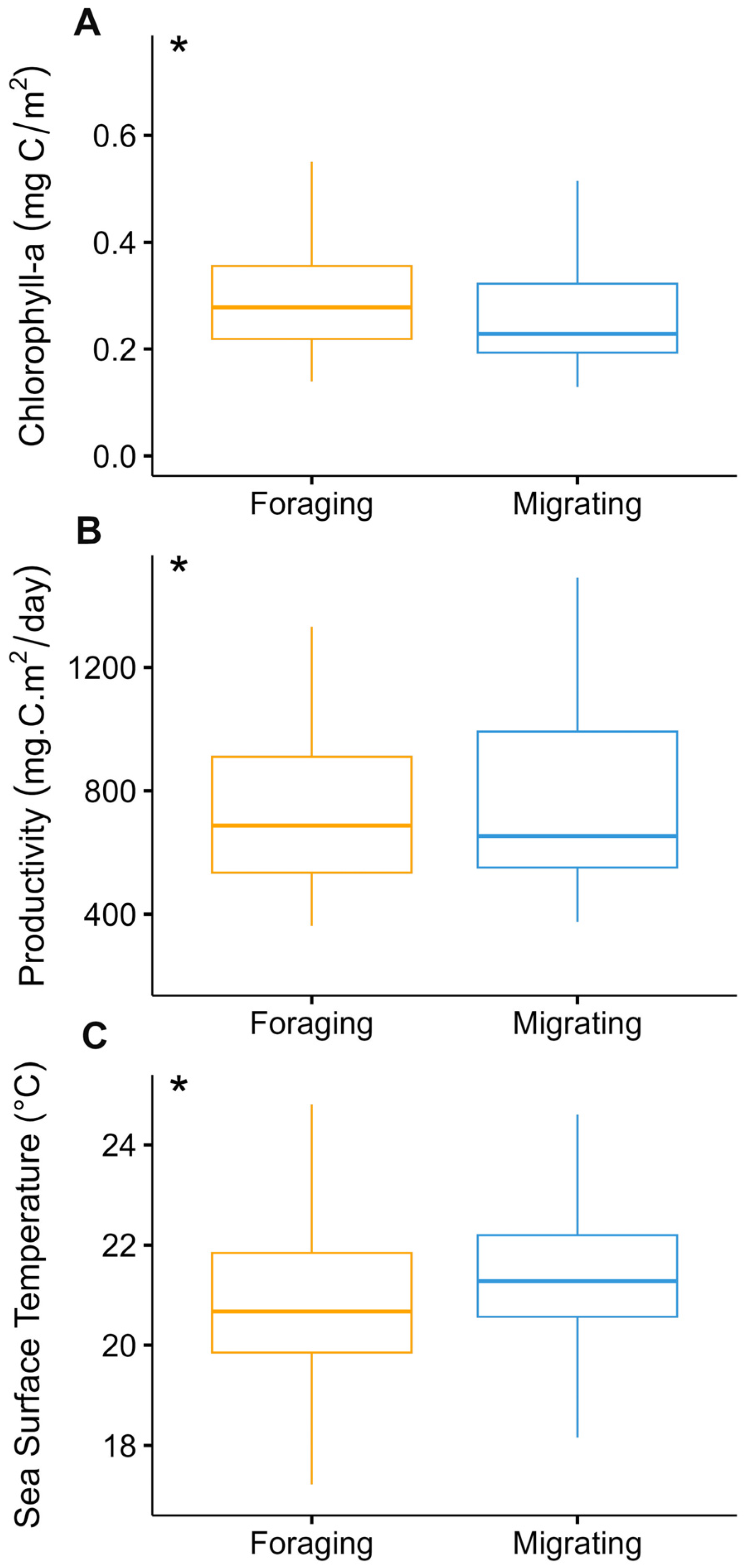
3.1. Identification of Behavioral States and Their Relationship with Environmental Variables
3.2. El Niño–Southern Oscillation
4. Discussion
5. Conclusions
Author Contributions
Funding
Institutional Review Board Statement
Informed Consent Statement
Data Availability Statement
Acknowledgments
Conflicts of Interest
References
- Jackson, J. Ecological extinction and evolution in the brave new ocean. Proc. Natl. Acad. Sci. USA 2008, 105 (Suppl. S1), 11458–11465. [Google Scholar] [CrossRef]
- O’Hara, C.; Frazier, M.; Halpern, B. At-risk marine biodiversity faces extensive, expanding, and intensifying human impacts. Science 2021, 372, 84–87. [Google Scholar] [CrossRef] [PubMed]
- Selig, E.; Turner, W.; Troëng, S.; Wallace, B.; Halpern, B.; Kaschner, K.; Lascelles, B.; Carpenter, K.; Mittermeier, R. Global priorities for marine biodiversity conservation. PLoS ONE 2014, 9, e82898. [Google Scholar] [CrossRef]
- Sandifer, P.; Sutton-Grier, A. Connecting stressors, ocean ecosystem services, and human health. Nat. Resour. Forum 2014, 38, 157–167. [Google Scholar] [CrossRef]
- Chami, R.; Cosimano, T.; Fullenkamp, C.; Oztosun, S. Nature’s solution to climate change. Financ. Dev. 2019, 56, 34–38. [Google Scholar]
- Menegotto, A.; Rangel, T. Mapping knowledge gaps in marine diversity reveals a latitudinal gradient of missing species richness. Nat. Commun. 2018, 9, 4713. [Google Scholar] [CrossRef]
- Attard, C.; Beheregaray, L.; Möller, L. Towards population-level conservation in the critically endangered Antarctic blue whale: The number and distribution of their populations. Sci. Rep. 2016, 6, 22291. [Google Scholar] [CrossRef]
- Cooke, J. Balaenoptera musculus (Errata Version Published in 2019). The IUCN Red List of Threatened Species. 2018. Available online: https://dx.doi.org/10.2305/IUCN.UK.2018-2.RLTS.T2477A156923585.en (accessed on 15 February 2019).
- Branch, T.A.; Matsuoka, K.; Miyashita, T. Evidence for increases in Antarctic blue whales based on Bayesian modelling. Mar. Mammal Sci. 2004, 20, 726–754. [Google Scholar] [CrossRef]
- Branch, T.; Stafford, K.; Palacios, D.; Allison, C.; Bannister, J.; Burton, C.; Cabrera, E.; Carlson, C.; Galletti Vernazzani, B.; Gill, P.; et al. Past and present distribution, densities and movements of blue whales Balaenoptera musculus in the Southern Hemisphere and northern Indian Ocean. Mammal Rev. 2007, 37, 116–175. [Google Scholar] [CrossRef]
- National Marine Fisheries Service. Draft Recovery Plan for the Blue Whale (Balaenoptera musculus)—Revision; National Marine Fisheries Service, Office of Protected Resources: Silver Spring, MD, USA, 2018.
- Reeves, R.; Clapham, P.; Brownell, R.; Silber, G. Recovery Plan for the Blue Whale (Balaenoptera musculus); Office of Protected Resources, National Marine Fisheries Service: Silver Spring, MD, USA, 1998; p. 42. [Google Scholar]
- Calambokidis, J.; Barlow, J. Abundance of blue and humpback whales in the eastern North Pacific estimated by capture-recapture and line-transect methods. Mar. Mammal Sci. 2004, 20, 63–85. [Google Scholar] [CrossRef]
- LeDuc, R.G.; Archer, E.; Lang, A.; Martien, K.; Hancock-Hanser, B.; Torres-Florez, J.; Hucke-Gaete, R.; Rosenbaum, H.; Van Waerebeek, K.; Brownell, R.; et al. Genetic variation in blue whales in the Eastern Pacific: Implication for taxonomy and use of common wintering grounds. Mol. Ecol. 2017, 26, 740–751. [Google Scholar] [CrossRef] [PubMed]
- Ichihara, T. The pygmy blue whale, Balaenoptera musculus brevicauda, a new subspecies from the Antarctic. In Whales, Dolphins, and Porpoises; Norris, K.S., Ed.; University of California Press: Berkeley, CA, USA, 1966; pp. 79–111. [Google Scholar]
- Rice, D. Marine Mammals of the World: Systematics and Distribution; The Society for Marine Mammalogy: Lawrence, KS, USA, 1998. [Google Scholar]
- Attard, C.; Beheregaray, L.; Jenner, K.; Gill, P.; Jenner, M.; Morrice, M.; Peter, R.; Möller, L. Low genetic diversity in pygmy blue whales is due to climate-induced diversification rather than anthropogenic impacts. Biol. Lett. 2015, 11, 20141037. [Google Scholar] [CrossRef]
- Anderson, R.; Branch, T.; Alagiyawadu, A.; Baldwin, R.; Marsac, F. Seasonal distribution, movements and taxonomic status of blue whales (Balaenoptera musculus) in the northern Indian Ocean. J. Cetacean Res. Manag. 2012, 12, 203–218. [Google Scholar] [CrossRef]
- International Whaling Commission. Report of the Scientific Committee. Available online: https://archive.iwc.int/pages/view.php?ref=19277&k= (accessed on 20 August 2021).
- Pastene, L.; Acevedo, J.; Branch, T. Morphometric analysis of Chilean blue whales and implications for their taxonomy. Mar. Mammal Sci. 2020, 36, 116–135. [Google Scholar] [CrossRef]
- Gambell, R. The Blue Whale. Biologist 1979, 26, 209–215. [Google Scholar]
- Donovan, G. A review of IWC stock boundaries. Rep. Int. Whal. Commn 1991, 13, 39–68. [Google Scholar]
- Torres-Florez, J.; Hucke-Gaete, R.; LeDuc, R.; Lang, A.; Taylor, B.; Pimper, L.; Bedriñana-Romano, L.; Rosenbaum, H.; Figueroa, C. Blue whale population structure along the eastern South Pacific Ocean: Evidence of more than one population. Mol. Ecol. 2014, 29, 5998–6010. [Google Scholar] [CrossRef]
- McDonald, M.; Mesnick, S.; Hildebrand, J. Biogeographic characterisation of blue whale song worldwide: Using song to identify populations. J. Cetacean Res. Manag. 2006, 8, 55–65. [Google Scholar] [CrossRef]
- Buchan, S.; Hucke-Gaete, R.; Rendell, L.; Stafford, K. A new song recorded from blue whales in the Corcovado Gulf, Southern Chile, and an acoustic link to the Eastern Tropical Pacific. Endanger. Spec. Res. 2014, 23, 241–252. [Google Scholar] [CrossRef]
- Barlow, D.; Klinck, H.; Ponirakis, D.; Holt Colberg, M.; Torres, L. Temporal occurrence of three blue whale populations in New Zealand waters from passive acoustic monitoring. J. Mammal. 2023, 104, 29–38. [Google Scholar] [CrossRef]
- Cerchio, S.; Willson, A.; Leroy, E.; Muirhead, C.; Al Harthi, S.; Baldwin, R.; Cholewiak, D.; Collins, T.; Minton, G.; Rasoloarijao, T.; et al. A new blue whale song-type described for the Arabian Sea and Western Indian Ocean. Endanger. Spec. Res. 2020, 43, 495–515. [Google Scholar] [CrossRef]
- Croll, D.; Marinovic, B.; Benson, S.; Chavez, F.; Black, N.; Tershy, B. From wind to whales: Trophic links in an upwelling ecosystem. Mar. Ecol. Prog. Ser. 2005, 289, 117–130. [Google Scholar] [CrossRef]
- Palacios, D. Blue whale (Balaenoptera musculus) occurrence off the Galapagos Islands, 1978–1995. J. Cetacean Res. Manag. 1999, 1, 41–51. [Google Scholar] [CrossRef]
- Kawamura, A. A review of food of balaenopterid whales. Sci. Rep. Whales Res. Inst. 1980, 32, 155–170. [Google Scholar]
- Reilly, S.B.; Thayer, V.G. Blue whale (Balaenoptera musculus) distribution in the Eastern Tropical Pacific. Mar. Mammal Sci. 1990, 6, 265–277. [Google Scholar] [CrossRef]
- Findlay, K.; Pitman, R.; Tsurui, T.; Sakai, K.; Ensor, P.; Iwakami, H.; Ljungblad, D.; Shimada, H.; Thiele, D.; Van Waerebeek, K.; et al. 1997/1998 IWC-Southern Ocean Whale and Ecosystem Research (IWC-SOWER) Blue Whale Cruise, Chile; Paper SC/50/Rep2 presented to the IWC Scientific Committee April 1998 (unpublished); International Whaling Commission: Muscat, Oman, 1998. [Google Scholar]
- Hucke-Gaete, R.; Bedrinana-Romano, L.; Viddi, F.; Ruiz, J.; Torres-Florez, J.; Zerbini, A. From Chilean Patagonia to Galapagos, Ecuador: Novel insights on blue whale migratory pathways along the Eastern South Pacific. PeerJ 2018, 6, e4695. [Google Scholar] [CrossRef]
- Sirovic, A.; Hildebrand, J.; Wiggins, S.; McDonald, M.; Moore, S.; Thiele, D. Seasonality of blue and fin whale calls west of the Antarctic Peninsula. Deep Sea Res. II 2004, 51, 2327–2344. [Google Scholar] [CrossRef]
- Samaran, F.; Adam, O.; Guinet, C. Discovery of a mid-latitude sympatric area for two Southern Hemisphere blue whale subspecies. Endanger. Spec. Res. 2010, 12, 157–165. [Google Scholar] [CrossRef]
- Denkinger, J.; Douglas, A.; Biggs, D.; Sears, R.; Narvaez, M.; Alarcon, D. Year-round presence of northern and southern hemisphere blue whales (Balaenoptera musculus) at the Galapagos Archipelago. J. Cetacean Res. Manag. 2023, 24, 63–76. [Google Scholar] [CrossRef]
- Stafford, K.; Bohnenstiehl, D.; Tolstoy, M.; Chapp, E.; Mellinger, D.; Moore, S. Antarctic-type blue whale calls recorded at low latitudes in the Indian and eastern Pacific Oceans. Deep Sea Res. I 2004, 51, 1337–1346. [Google Scholar] [CrossRef]
- Stafford, K.; Nieukirk, S.; Fox, C. An acoustic link between blue whales in the eastern tropical Pacific and the northeast Pacific. Mar. Mammal Sci. 1999, 15, 1258–1268. [Google Scholar] [CrossRef]
- Guzman, H.M.; Estévez, R.M. Connectivity between Northeast and Southeast Pacific blue whale populations in the Galapagos Archipelago. Mar. Mammal Sci. 2024; in press. [Google Scholar]
- Alarcón-Ruales, D.; Denkinger, J.; Zurita-Arthos, L.; Herrera, S.; Díaz-Pazmiño, S.; Espinoza, E.; Muñoz Pérez, J.P.; Holmes, B.J.; Townsend, K.A. Cetaceans of the Galapagos Archipelago: Species in Constant Change and the Importance of a Standardized and Long-Term Citizen Science Program. In Island Ecosystems: Challenges to Sustainability; Springer International Publishing: Cham, Switzerland, 2023; pp. 335–355. [Google Scholar]
- Guzman, H.M.; Gómez, C.; Guevara, C.; Kleivane, L. Potential vessel collisions with Southern Hemisphere humpback whales wintering off Pacific Panama. Mar. Mammal Sci. 2013, 29, 629–642. [Google Scholar] [CrossRef]
- Kleivane, L.; Kvadsheim, P.H.; Bocconcelli, A.; Øien, N.; Miller, P. Equipment to tag, track and collect biopsies from whales and dolphins: The ARTS, DFHorten and LKDart systems. Anim. Biotelemetry 2022, 10, 32. [Google Scholar] [CrossRef]
- Vincent, C.; McConnell, B.J.; Ridoux, V.; Fedak, M. Assessment of Argos location accuracy from satellite tags deployed on captive gray seals. Mar. Mammal Sci. 2002, 18, 156–166. [Google Scholar] [CrossRef]
- Guzman, H.M.; Félix, F. Movements and habitat use by Southeast Pacific humpback whales (Megaptera novaeangliae) satellite tracked at two breeding sites. Aquat. Mamm. 2017, 43, 139. [Google Scholar] [CrossRef]
- Douglas, D.C.; Weinzierl, R.; Davidson, S.C.; Kays, R.; Wikelski, M.; Bohrer, G. Moderating Argos location errors in animal tracking data. Methods Ecol. Evol. 2012, 3, 999–1007. [Google Scholar] [CrossRef]
- Hucke-Gaete, R.; Osman, L.; Moreno, C.; Findlay, K.; Ljungblad, D. Discovery of a blue whale feeding and nursing ground in southern Chile. Proc. R. Soc. Lond. B 2004, 271 (Suppl. S4), S1. [Google Scholar] [CrossRef]
- Jonsen, I.; McMahon, C.; Patterson, T.; Auger-Méthé, M.; Harcourt, R.; Hindell, M.; Bestley, S. Movement responses to environment: Fast inference of variation among southern elephant seals with a mixed effects model. Ecology 2019, 100, e02566. [Google Scholar] [CrossRef]
- Jonsen, I.; Grecian, W.; Phillips, L.; Carroll, G.; McMahon, C.; Harcourt, R.; Hindell, M.; Patterson, T. aniMotum, an R package for animal movement data: Rapid quality control, behavioral estimation and simulation. Methods Ecol. Evol. 2023, 17, 806–816. [Google Scholar] [CrossRef]
- R Core Team. R: A Language and Environment for Statistical Computing; R Foundation for Statistical Computing: Vienna, Austria, 2024; Available online: www.R-project.org/ (accessed on 1 February 2024).
- Michelot, T.; Langrock, R.; Patterson, T. moveHMM: An R package for the statistical modelling of animal movement data using hidden Markov models. Methods Ecol. Evol. 2016, 7, 1308–1315. [Google Scholar] [CrossRef]
- Mendelssohn, R. Xtractomatic: Accessing Environmental Data from ERD’s ERDDAP Server, R Package Version 3.4.2. 2018. Available online: https://cran.r-project.org/src/contrib/Archive/xtractomatic/ (accessed on 1 February 2024).
- Mayer, L.; Jakobsson, M.; Allen, G.; Dorschel, B.; Falconer, R.; Ferrini, V.; Lamarche, G.; Snaith, H.; Weatherall, P. The nippon foundation—GEBCO seabed 2030 project: The quest to see the world’s oceans completely mapped by 2030. Geosciences 2018, 8, 63. [Google Scholar] [CrossRef]
- Irvine, L.M.; Mate, B.R.; Winsor, M.H.; Palacios, D.M.; Bograd, S.J.; Costa, D.P.; Bailey, H. Spatial and temporal occurrence of blue whales off the US West Coast, with implications for management. PLoS ONE 2014, 9, e102959. [Google Scholar] [CrossRef] [PubMed]
- Nickels, C.F.; Sala, L.M.; Ohman, M.D. The euphausiid prey field for blue whales around a steep bathymetric feature in the southern California current system. Limnol. Oceanogr. 2019, 64, 390–405. [Google Scholar] [CrossRef]
- Benson, S.R.; Croll, D.A.; Marinovic, B.B.; Chavez, F.P.; Harvey, J.T. Changes in the cetacean assemblage of a coastal upwelling ecosystem during El Niño 1997–98 and La Niña 1999. Progr. Oceanogr. 2002, 54, 279–291. [Google Scholar] [CrossRef]
- Torres, L.G.; Barlow, D.R.; Hodge, K.; Klinck, H.; Steel, D.; Baker, C.S.; Chandler, T.; Gill, P.; Ogle, M.; Lilley, C.; et al. New Zealand blue whales: Recent findings and research progress. J. Cetacean Res. Manag. 2017, 1–22. [Google Scholar]
- Palacios, D.M. Marine Mammal Research in the Galápagos Islands: The 1993–1994 Odyssey Expedition; Galápagos National Park Service and Charles Darwin Research Station: Puerto Ayora, Galápagos, Ecuador, 1999. [Google Scholar]
- Denkinger, J.; Oña, J.; Alarcón, D.; Merlen, G.; Salazar, S.; Palacios, D.M. From whaling to whale watching: Cetacean presence and species diversity in the Galápagos Marine Reserve. In Science and Conservation in the Galapagos Islands: Frameworks & Perspectives; Harpp, K.S., Ed.; Springer: New York, NY, USA, 2013; pp. 217–235. [Google Scholar]
- Palacios, D.M.; Cantor, M. Priorities for ecological research on cetaceans in the Galápagos Islands. Front. Mar. Sci. 2023, 10, 1084057. [Google Scholar] [CrossRef]
- Forryan, A.; Naveira Garabato, A.C.; Vic, C.; Nurser, A.G.; Hearn, A.R. Galápagos upwelling driven by localized wind–front interactions. Sci. Rep. 2021, 11, 1277. [Google Scholar] [CrossRef]
- Palacios, D.M. Seasonal patterns of sea-surface temperature and ocean color around the Galapagos: Regional and local influences. Deep-Sea Res. II 2004, 51, 43–57. [Google Scholar] [CrossRef]
- Alava, J.J. Carbon productivity and flux in the marine ecosystems of the Galapagos Marine Reserve based on cetacean abundances and trophic indices. Rev. Biol. Mar. Oceanogr. 2009, 44, 109–122. [Google Scholar] [CrossRef]
- Abrahms, B.; Hazen, E.L.; Aikens, E.O.; Savoca, M.S.; Goldbogen, J.A.; Bograd, S.J.; Mate, B.R. Memory and resource tracking drive blue whale migrations. Proc. Natl. Acad. Sci. USA 2019, 116, 5582–5587. [Google Scholar] [CrossRef]
- Ryan, J.P.; Benoit-Bird, K.J.; Oestreich, W.K.; Leary, P.; Smith, K.B.; Waluk, C.M.; Goldbogen, J.A. Oceanic giants dance to atmospheric rhythms: Ephemeral wind-driven resource tracking by blue whales. Ecol. Lett. 2022, 25, 2435–2447. [Google Scholar] [CrossRef]
- Rennie, S.; Hanson, C.E.; McCauley, R.D.; Pattiaratchi, C.; Burton, C.; Bannister, J.; Jenner, C.; Jenner, M.N. Physical properties and processes in the Perth Canyon, Western Australia: Links to water column production and seasonal pygmy blue whale abundance. J. Mar. Syst. 2009, 77, 21–44. [Google Scholar] [CrossRef]
- Lesage, V.; Gavrilchuk, K.; Andrews, R.D.; Sears, R. Foraging areas, migratory movements and winter destinations of blue whales from the western North Atlantic. Endanger. Spec. Res. 2017, 34, 27–43. [Google Scholar] [CrossRef]
- Prieto, R.; Tobeña, M.; Silva, M.A. Habitat preferences of baleen whales in a mid-latitude habitat. Deep-Sea Res. II 2017, 141, 155–167. [Google Scholar] [CrossRef]
- Derville, S.; Torres, L.G.; Zerbini, A.N.; Oremus, M.; Garrigue, C. Horizontal and vertical movements of humpback whales inform the use of critical pelagic habitats in the western South Pacific. Sci. Rep. 2020, 10, 4871. [Google Scholar] [CrossRef] [PubMed]
- Genin, A. Bio-physical coupling in the formation of zooplankton and fish aggregations over abrupt topographies. J. Mar. Syst. 2004, 50, 3–20. [Google Scholar] [CrossRef]
- Santora, J.A.; Zeno, R.; Dorman, J.G.; Sydeman, W.J. Submarine canyons represent an essential habitat network for krill hotspots in a large marine ecosystem. Sci. Rep. 2018, 8, 7579. [Google Scholar] [CrossRef]
- Luschi, P. Long-distance animal migrations in the oceanic environment: Orientation and navigation correlates. Int. Schol. Res. Notices 2013, 2013, 631839. [Google Scholar] [CrossRef]
- Thouless, C. Where the Whales Go: The Migration Routes of Humpbacks in the South West Atlantic. Master’s Thesis, The University of California, San Diego, CA, USA, 2021. Available online: https://escholarship.org/uc/item/1693m1b5 (accessed on 15 June 2024).
- Hucke-Gaete, R.; Lobo, A.; Yancovic-Pakarati, S.; Flores, M. Mamíferos marinos de la isla de pascua (Rapa Nui) e isla Salas y Gómez (Motu Motiro Hiva), Chile: Una revisión y nuevos registros. Lat. Am. J. Aquat. Res. 2014, 42, 743–751. [Google Scholar] [CrossRef]
- Buchan, S.; Hucke-Gaete, R.; Stafford, K.M.; Clark, C.W. Occasional acoustic presence of Antarctic blue whales on a feeding ground in southern Chile. Mar. Mammal Sci. 2017, 34, 440–458. [Google Scholar] [CrossRef]
- Convention on Biological Diversity (CBD). Ecologically or Biologically Significant Areas (EBSAs). 2017. Available online: https://chm.cbd.int/database/record?documentID=204100 (accessed on 10 June 2024).
- Massing, J.C.; Schukat, A.; Auel, H.; Auch, D.; Kittu, L.; Pinedo Arteaga, E.L.; Hagen, W. Toward a solution of the “Peruvian Puzzle”: Pelagic food-web structure and trophic interactions in the northern Humboldt current upwelling system off Peru. Front. Mar. Sci. 2022, 8, 759603. [Google Scholar] [CrossRef]
- Daneri, G.; Dellarossa, V.; Quiñones, R.; Jacob, B.; Montero, P.; Ulloa, O. Primary production and community respiration in the Humboldt Current System off Chile and associated oceanic areas. Mar. Ecol. Prog. Ser. 2000, 197, 41–49. [Google Scholar] [CrossRef]
- Faul, K.L.; Ravelo, A.C.; Delaney, M.L. Reconstructions of upwelling, productivity, and photic zone depth in the eastern equatorial Pacific Ocean using planktonic foraminiferal stable isotopes and abundances. J. Foraminifer. Res. 2000, 30, 110–125. [Google Scholar] [CrossRef]
- Buchan, S.J.; Quiñones, R.A. First insights into the oceanographic characteristics of a blue whale feeding ground in northern Patagonia, Chile. Mar. Ecol. Prog. Ser. 2016, 554, 183–199. [Google Scholar] [CrossRef]
- Buchan, S.J.; Pérez-Santos, I.; Narváez, D.; Castro, L.; Stafford, K.M.; Baumgartner, M.F.; Valle-Levinson, A.; Montero, P.; Gutiérrez, L.; Rojas, C.; et al. Intraseasonal variation in southeast Pacific blue whale acoustic presence, zooplankton backscatter, and oceanographic variables on a feeding ground in Northern Chilean Patagonia. Progr. Oceanogr. 2021, 199, 102709. [Google Scholar] [CrossRef]
- Hazen, E.L.; Friedlaender, A.S.; Goldbogen, J.A. Blue whales (Balaenoptera musculus) optimize foraging efficiency by balancing oxygen use and energy gain as a function of prey density. Sci. Adv. 2015, 1, e1500469. [Google Scholar] [CrossRef] [PubMed]
- Palacios, D.M.; Bailey, H.; Becker, E.A.; Bograd, S.J.; DeAngelis, M.L.; Forney, K.A.; Mate, B.R. Ecological correlates of blue whale movement behavior and its predictability in the California Current Ecosystem during the summer-fall feeding season. Mov. Ecol. 2019, 7, 26. [Google Scholar] [CrossRef]
- Szesciorka, A.R.; Ballance, L.T.; Širović, A.; Rice, A.; Ohman, M.D.; Hildebrand, J.A.; Franks, P.J.S. Timing is everything: Drivers of interannual variability in blue whale migration. Sci. Rep. 2020, 10, 7710. [Google Scholar] [CrossRef]
- Oestreich, W.K.; Abrahms, B.; McKenna, M.F.; Goldbogen, J.A.; Crowder, L.B.; Ryan, J.P. Acoustic signature reveals blue whales tune life-history transitions to oceanographic conditions. Funct. Ecol. 2022, 36, 882–895. [Google Scholar] [CrossRef]
- Lee, T.; McPhaden, M.J. Increasing intensity of El Niño in the central-equatorial Pacific. Geophys. Res. Lett. 2010, 37, L14603. [Google Scholar] [CrossRef]
- Truong, G.; Rogers, T.L. La Niña conditions influence interannual call detections of pygmy blue whales in the eastern Indian Ocean. Front. Mar. Sci. 2023, 9, 850162. [Google Scholar] [CrossRef]
- Denkinger, J.; Parra, M.; Muñoz, J.P.; Carrasco, C.; Murillo, J.C.; Espinosa, E.; Koch, V. Are boat strikes a threat to sea turtles in the Galapagos Marine Reserve? Ocean Coast. Manag. 2013, 80, 29–35. [Google Scholar] [CrossRef]
- Ransome, N.; Loneragan, N.R.; Medrano-González, L.; Félix, F.; Smith, J.N. Vessel strikes of large whales in the eastern tropical Pacific: A case study of regional underreporting. Front. Mar. Sci. 2021, 8, 675245. [Google Scholar] [CrossRef]
- Sitar, A.; McCauley, L.J.; Wright, A.J.; Peters-Burton, E.; Rockwood, L.; Parsons, E.C.M. Boat operators in Bocas del Toro, Panama display low levels of compliance with national whale-watching regulations. Mar. Policy 2016, 68, 221–228. [Google Scholar] [CrossRef]
- Guzman, H.M.; Hinojosa, N.; Kaiser, S. Ship’s compliance with a traffic separation scheme and speed limit in the Gulf of Panama and implications for the risk to humpback whales. Mar. Policy 2020, 120, 104113. [Google Scholar] [CrossRef]

| Id | Tagging Date (mm-dd-yyyy) | Last Date (mm-dd-yyyy) | Transmissions (Days) | Traveled Distance (km) | EEZ (Days) |
|---|---|---|---|---|---|
| 178968 | 10-02-2021 | 08-01-2022 | 98.13 | 11,395.47 | 23.08 |
| 178970 | 10-03-2021 | 08-30-2022 | 331.91 | 4341.43 | 4.04 |
| 178972 | 08-03-2021 | 09-27-2021 | 54.55 | 1045.77 | 54.55 |
| 196849 | 10-07-2021 | 10-20-2021 | 13.59 | 4262.14 | 13.59 |
| 196850 | 10-04-2021 | 11-08-2021 | 34.99 | 3471.42 | 33.88 |
| 196852 | 10-04-2021 | 11-15-2021 | 42.15 | 3228.02 | 12.04 |
| 196853 | 10-02-2021 | 10-29-2021 | 27.49 | 3324.29 | 13.02 |
| 196854 | 10-05-2021 | 11-03-2021 | 28.82 | 3138.75 | 28.82 |
| 196855 | 10-02-2021 | 10-27-2021 | 24.52 | 2004.12 | 24.52 |
| 196856 | 11-06-2021 | 01-01-2022 | 56.00 | 4026.65 | 26.32 |
| 178971 | 09-26-2022 | 10-01-2022 | 5.15 | 2369.53 | 5.15 |
| 196860 | 10-06-2022 | 11-18-2022 | 43.00 | 3139.70 | 43.00 |
| 228112 | 10-01-2022 | 11-04-2022 | 34.45 | 3076.18 | 28.83 |
| 228114 | 10-14-2022 | 10-29-2022 | 14.49 | 1424.57 | 1.94 |
| 228115 | 09-27-2023 | 11-03-2023 | 37.51 | 2508.08 | 37.51 |
| 228119 | 09-23-2023 | 10-17-2023 | 23.77 | 2675.84 | 17.4 |
| Model Parameter | Behavioral State | Value |
|---|---|---|
| Step Length (km) | Migratory | 60 ± 10 |
| Foraging | 20 ± 10 | |
| Turning Angle | Migratory | 0 |
| Foraging | π |
| Depth (m) | Foraging (%) | Migrating (%) |
|---|---|---|
| 0–200 | 6.44 | 8.14 |
| 201–500 | 2.21 | 8.35 |
| 501–1000 | 5.63 | 6.59 |
| 1001–1500 | 3.42 | 6.37 |
| >1500 | 82.30 | 70.55 |
| From Foraging to Migrating State | From Migrating to Foraging State | |
|---|---|---|
| Intercept | −1.957 (−2.354, −1.560) | −2.569 (−2.963, −2.174) |
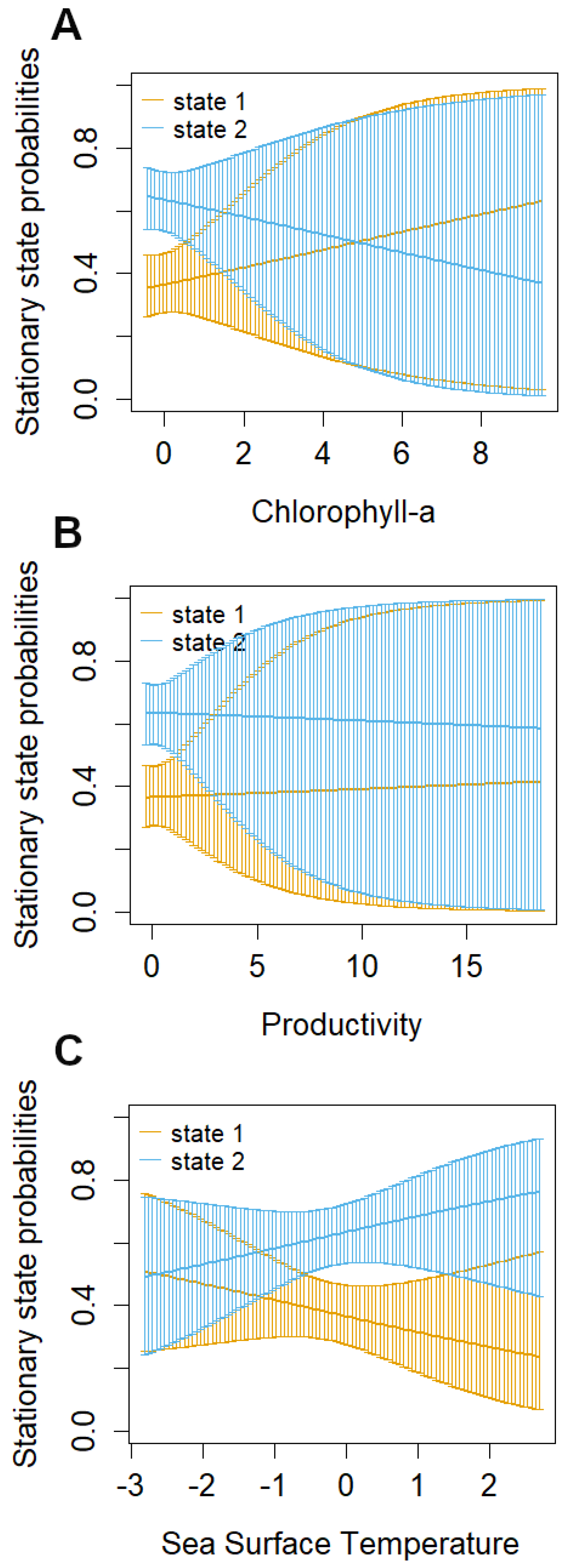
| Chl | −0.069 (−0.415, 0.276) | 0.057 (−0.347, 0.460) |
| Prod | 0.062 (−0.166, 0.290) | 0.070 (−0.228, 0.368) |
| SST | −0.174 (−0.545, 0.197) | −0.405 (−0.895, 0.085) |
Disclaimer/Publisher’s Note: The statements, opinions and data contained in all publications are solely those of the individual author(s) and contributor(s) and not of MDPI and/or the editor(s). MDPI and/or the editor(s) disclaim responsibility for any injury to people or property resulting from any ideas, methods, instructions or products referred to in the content. |
© 2024 by the authors. Licensee MDPI, Basel, Switzerland. This article is an open access article distributed under the terms and conditions of the Creative Commons Attribution (CC BY) license (https://creativecommons.org/licenses/by/4.0/).
Share and Cite
Guzman, H.M.; Estévez, R.M.; Kaiser, S. Insights into Blue Whale (Balaenoptera musculus L.) Population Movements in the Galapagos Archipelago and Southeast Pacific. Animals 2024, 14, 2707. https://doi.org/10.3390/ani14182707
Guzman HM, Estévez RM, Kaiser S. Insights into Blue Whale (Balaenoptera musculus L.) Population Movements in the Galapagos Archipelago and Southeast Pacific. Animals. 2024; 14(18):2707. https://doi.org/10.3390/ani14182707
Chicago/Turabian StyleGuzman, Hector M., Rocío M. Estévez, and Stefanie Kaiser. 2024. "Insights into Blue Whale (Balaenoptera musculus L.) Population Movements in the Galapagos Archipelago and Southeast Pacific" Animals 14, no. 18: 2707. https://doi.org/10.3390/ani14182707
APA StyleGuzman, H. M., Estévez, R. M., & Kaiser, S. (2024). Insights into Blue Whale (Balaenoptera musculus L.) Population Movements in the Galapagos Archipelago and Southeast Pacific. Animals, 14(18), 2707. https://doi.org/10.3390/ani14182707