Article

Integration of Thermal Core Profiling and Scratch Testing for the Study of Unconventional Reservoirs

1
Center for Hydrocarbon Recovery, Skolkovo Institute of Science and Technology, 30/1 Bolshoy Boulevard, 121205 Moscow, Russia
2
LLC Gazpromneft Scientific and Technical Center, 75-79D Moika River Emb., 190000 St. Petersburg, Russia
*
Author to whom correspondence should be addressed.
Geosciences 2021, 11(6), 260; https://doi.org/10.3390/geosciences11060260
Submission received: 9 May 2021 / Revised: 9 June 2021 / Accepted: 14 June 2021 / Published: 17 June 2021
(This article belongs to the Special Issue Petrophysics and Geochemistry of Unconventional Reservoirs)

Abstract

:
Core analysis provides the essential information necessary for the characterization and development of hydrocarbon reservoirs. High core-scale heterogeneity and anisotropy, natural in unconventional reservoirs, complicate reservoir characterization and dictate the sampling methodology used. Continuous high-resolution thermal measurements with an optical scanner and scratcher along the core column can yield benefits in a sampling strategy. This article describes some features of the suggested integration of non-destructive thermal profiling with partially destructive scratch testing applied for the study of rocks from the Bazhenov Formation (West Siberia, Russia). The spatial variation in the unconfined compressive strength and thermal conductivity components parallel and perpendicular to bedding for more than 1000 samples are demonstrated and discussed on core and log scales. The relationships between these properties are established for different rock types composing the formation. The joint analysis allows specialists to correctly define multiscale heterogeneities and facies that would be difficult or impossible to observe with logging data analysis or geological description alone. The established relationships make it possible to partially replace the semi-destructive scratch test with non-destructive optical scanning, providing UCS estimation. One more important outcome of the present work is the lessons learned regarding how to organize future works. The integration of thermal core profiling and scratch testing data looks promising for unconventional reservoir characterization.

1. Introduction

One of the most significant issues in unconventional reservoirs, particularly in tight gas/oil reservoirs and gas/oil shales, is their heterogeneity and anisotropy. This significantly complicates reservoir characterization by influencing the selection of representative core collection for further study in a laboratory and thereby the core analysis results [1,2,3]. The composition and microstructure may vary significantly from the cm- to mm scale in unconventional reservoir rocks [2], reflecting the variable depositional conditions. Shale rocks are generally regarded as a transversely isotropic material, with anisotropy caused by the preferred orientation of clay minerals, kerogen layers, and the presence of fluid-filled microcracks [3]. Accounting for rock heterogeneity and anisotropy is especially important for the comprehensive laboratory testing of rock mechanics [2,4], which is expensive, time-consuming, and unique because it results in core destruction. The improper sampling of cores from such formations can result in a biased representation of the formation [4].
Heterogeneity is defined by the spatial variability in rock texture and composition and can be quantified and tracked at different scales (core, logging, or seismic). Fine-scale heterogeneity over the core column length can be described via CT scanning [1,5], scratch testing [4,6,7,8,9], and thermal core profiling [10,11,12]. CT scanning provides a quantitative evaluation of the X-ray attenuation number (related to the density and atomic number). It has problems with distinguishing micropores and microfractures in full-size cores [5], which is essential for geomechanical study. The scratch test [4,6,7,8,13] provides a measure of the specific energy (which relates to UCS, unconfined compressive strength) required for sample destruction. It is partially destructive and, as a result, rarely carried out in practice for samples/rock types extremely sensitive for mechanical treatment. Continuous high-resolution (0.2–2 mm) thermal profiling along a core sample column provides measurements of the fundamental (thermal) physical properties of rocks, accounting for anisotropy in a non-contact, non-destructive manner right at the core storages [11,12].
These features of thermal profiling combined with established strong correlations between thermal and cross-dipole sonic logging data [14] (as well as between sonic logging data and UCS [15,16]) makes the integration of thermal core profiling and scratch testing promising for reservoir characterization [17]. The first attempts to jointly analyze the profiles of thermal conductivity and UCS on separate samples (see the example for the sillimanite-biotite shist sample [9]) showed that two different physical profiles—thermal and mechanical—complement one another and provide much richer information about rock heterogeneity than only one profile. Moreover, there are no dependencies between these properties in [9], since the work is aiming to determine the relationship between the two types of measurements. The relationship between thermal conductivity and UCS presented in [18] is very general because it is built using individual values for a diverse collection of samples consisting of eight sedimentary and igneous rock types in dry conditions. However, trends can strongly vary from one rock type to another and from one well to another—i.e., empirical laws relating strength with other petrophysical properties are not universal and must be handled with care [9,19]. For unconventional reservoirs, a general link between vertical variations in the UCS and the thermal conductivity component perpendicular to bedding was established (after data upscaling) in the lower part of the Bazhenov Formation. However, the regression analysis of the thermal conductivity and UCS was not performed either on individual samples or along the well, and the link causes were not discussed [20].
This paper aims to demonstrate, for the first time, the features of the integration of thermal core profiling and scratch testing data using the example of unconventional reservoir rocks from the Bazhenov Formation (West Siberia, Russia) on core and logging scales. It includes a heterogeneity analysis of studied rocks, an analysis of the “thermal conductivity–UCS” relationships for both separate core samples and different rock types, and a description of the lessons we learned to help future researchers in this area.

2. Materials and Methods

2.1. Study Object and Materials

Our research objects are rocks from the Bazhenov Formation, predominantly biogenic deposits from the Upper Jurassic period, and are considered the primary source rock of the Western Siberian Basin [21,22,23]. More than 1000 full-diameter core samples obtained at three wells of an oilfield in the central part of the basin were slabbed and profiled using an optical scanner and scratcher. The studied deposits are composed of siliceous, clayey, and carbonate minerals in various proportions (details on the mineral compositions can be found in [14]). The rocks are rich in planktonic type II organic matter; the total organic carbon (TOC) content in the studied rocks reaches up to 24%. Organic matter is present in the rock as ultra-fine stringers, thin, indistinct horizontally layered, and lenticular interlayers that penetrate the rock matrix with thin inclusions. The rock permeability varies from 0.001 to 0.975 mD, with an average value of 0.064 mD, while the connected porosity (measured with helium) varies from 0.33 to 6.95%, with an average value of 1.10% [14]. The value of the total porosity is approximately four times greater than that of the connected porosity [24].
Specialists classified the deposits into five lithophysical types (Table 1) based on the analysis of well logging data and the results of lithological description [25]. Rocks containing more than 50% siliceous minerals were denoted as silicites (1) or clayey silicites (2) if they featured a clay component in a proportion of greater than 10%. Carbonate rocks (3) are composed mainly of calcite or dolomite and may contain a siliceous and clay component in a proportion of less than 10%; if the content of siliceous minerals is greater than 10%, specialists classify it as a siliceous-carbonate rock. Clayey-siliceous-carbonate deposits (4) denote rocks with a content of carbonate minerals higher than that found in siliceous rocks, a siliceous content higher than the clay mineral content, and a content of clay minerals exceeding 10%. Clayey-siliceous rocks (5) are composed of siliceous (up to 50%) and clay (up to 30%) minerals, and the content of any other mineral component does not exceed 10%. Rocks are denoted additionally depending on their TOC values as either low carbonaceous (0–5% TOC), carbonaceous (5–10% TOC), or highly carbonaceous rocks (TOC > 10%).
The results of the thin section analysis and data on the key elements and mineralogy obtained using a high-definition spectroscopy tool (LithoScanner with a vertical resolution of 45.72 cm [26]) are also used.

2.2. Scratch Test Data

Scratch testing [4,6,7,8,9,13] was performed before this study in a special geomechanical laboratory. The method is based on cutting (scratching) the rock surface with a cutter moving with a constant velocity along the core sample surface, measuring the normal and tangential forces, determining the specific energy required to create continuous failure, and calculating the UCS. The mechanics of the scratching are described in [6,8]. UCS profiles were obtained with 0.1 mm steps without any information about their metrological characteristics—signal-to-noise ratio (that is so-called dynamic range), precision, accuracy, and uncertainty. It is necessary to add that the metrology is absent in the vast majority of publications featuring scratching results (to our knowledge only Richard et al. [8] provided an estimation of dispersion in the results of the scratching of Vosges sandstone). According to our experimental estimates, the dynamical range (ratio of useful signal range to a noise value) for an optical scanner is 3 to 10 times higher than the dynamical range of the scratcher. This is why, for the noise reduction and convenience of analysis with thermal profiling data, we upscaled the results of scratching using the moving average filter with the window of 1 mm, which essentially improved the dynamic range of the scratcher.

2.3. Thermal Profiling Data

Thermal profiling was carried out in core storage using the optical scanning instrument. The instrument includes an immovable platform with rock samples and two reference samples (with known thermal properties), a movable optical head with a focused, mobile, and continuously operated optical heat source, and three infrared temperature sensors [11]. In this study, the heat source is a special electric lamp providing a heat spot (of 6–7 mm in diameter) on the surface of rock samples, which are placed on the platform. During the core scanning, the optical head is moving with constant velocity (adjustable parameter, 1–10 mm/s), and the temperature responses from the rock samples and two reference samples are registered on the fixed distance from the heat spot center (adjustable parameter, 20–50 mm). Power of the heat source, scanning velocity, and the distance is set to provide a balance between speed of investigation, depth of investigation and spatial resolution, a maximum temperature of heating (important for unconventional formations and liquid-saturated rocks), and measurement quality depending on the research goal. Measured excessive temperature is transformed to thermal conductivity; thermal diffusivity; and, as a result, volumetric heat capacity using the solution of the thermal diffusivity equation for a quasi-stationary temperature field in a movable coordinate system. All necessary information including a description of the experimental setup and technical parameters, theoretical background, measurement procedure, and data processing can be found in [11]. The instrument used in this study provides a spatial resolution of ~1 mm to fix rock thermal heterogeneity.
In special cases, a laser optical scanning instrument can be used to provide better special resolution (up to 0.2 mm) where the distance between the laser spot and field of view of infrared sensors is about 3 mm [10].
The method is universally recognized, has been thoroughly tested, and is included in the ISRM (the International Society for Rock Mechanics and Rock Engineering) suggested methods for determining the thermal properties of rocks [11]. The total uncertainty (combination of systematic and random error) in thermal conductivity measurements does not exceed ±2.5% at a confidence level of 0.95. The equipment used in this study is described in [14] along with the corresponding thermal property data from three wells (A, B, and C). Most of the core samples were scanned twice in two mutually perpendicular directions that allowed us to determine two thermal conductivity tensor components: along (λ||) and perpendicular (λ) to the bedding plane (the Bazhenov Formation can be considered as the transverse isotropy medium with a vertical axis of symmetry [2,14]).

2.4. Workflow

Before the present study, most of the full-size cylindrical core samples extracted from the Bazhenov Formation (Figure 1a) were slabbed (split) longitudinally into two parts (the major one had a thickness of approximately 2/3 of the core diameter, while the minor one had a thickness of approximately 1/3 of the core diameter). A scratch test performed on the cylindrical surface (Figure 1b) in a laboratory outside the core storage resulted in partial core disintegration (Figure 1b,c). As an example, Figure 1e,f shows that a core sample (represented by a layering of siliceous and clayey-siliceous carbonaceous rocks) from interval xx69.38–xx69.68 m of well A was disintegrated as a result of scratching into four samples along planes parallel to the bedding plane. The scratch test measurements result in UCS profiles that are correlated to the actual UCS tests made by geomechanical testing [20]. After the scratch test, plugs were drilled out for geomechanical study, and the core was returned to the core storage. After a while, we performed thermophysical profiling in the core storage; the vast majority of the samples were profiled along the major part of split cores (see Figure 1c,f). We choose the parts of cores with satisfactory length during profiling to get representative information on core heterogeneity. An example is shown in Figure 1c: instead of scanning two major parts, one of which has a hole after plug drilling, we scanned an unbroken minor part corresponding to these two major parts.
The obtained UCS and thermal conductivity profiles correlate with each other in general (Figure 1d). Unfortunately, the precise alignment (correlation) of the thermal conductivity and UCS profiles of every scanned sample could not be conducted for several reasons: scratching and thermophysical profiling were carried out several years ago by different groups of specialists in different places, at different times, on different parts of the samples (sometimes with different lengths). We control and correct depth adjustment by matching core photos before scratching (with overlaid UCS profiles) to core photos before optical scanning (with overlaid thermal conductivity profiles). The high heterogeneity of the samples and the absence of an accurate (with an accuracy to the nearest millimeter) correlation of the depth profiles for most of the samples significantly complicates the subsequent joint analysis of the data obtained. A shift in one profile by several centimeters relative to another can lead to the “blurring” of the possible correlation dependence when analyzing the data (as can be seen from Figure 1d). Moreover, the joint analysis of the profiles on small scales (from several millimeters to centimeters) is complicated by the lack of mentioned above metrological characteristics of the scratcher. This is why we firstly selected data on several samples that satisfy two conditions:
  • The presence of the results of petrographic analysis on the thin sections in the depth interval with the presence of UCS and thermal conductivity profiles;
  • The ability to link (adjust) these profiles with each other in-depth, taking into account core heterogeneity.
Secondly, for a comprehensive analysis, the initial data (UCS, thermal conductivity components along and across the bedding) were averaged in a movable 30 cm window with the middle of the averaging window referenced to the middle of each core sample. Additionally, core–log integration (transformation of core depth to logging depth) was performed to include the results of lithophysical typing and LithoScanner data in the analysis.

3. Results

3.1. Profiles along the Wells

The results of the thermal conductivity and UCS profiling are presented along with the results of the lithophysical rock typing in Figure 2. In general, an increase in thermal conductivity with an increase in the UCS was observed. However, there is no unique relationship between the thermal conductivity of rocks and UCS, since these properties of rocks are influenced to varying degrees by various factors, as discussed in Section 4.1.
Profiling statistics (Figure 3) show that 99.5% of the thermal conductivity values of the studied rocks lie within the range of 0.75–3.2 W·m−1·K−1, while 99.5% of the UCS values are below 243 MPa. Here, ‘PDF’ represents an estimate of probability density function (the area of each bar is the relative number of observations, the sum of the bar areas is 1), where the number of bins was chosen according to Scott’s rule [27]. The value of the thermal inhomogeneity coefficient β in 99 cases out of 100 lies in the range of 0.03–0.87, the average value X is 0.18 (standard deviation = 0.13), and the average length of the samples studied by the optical scanning method is 57 mm (standard deviation = 29 mm). The thermal heterogeneity factor was determined for the thermal conductivity profile of each core sample by the formula in Figure 3c, where λmini and λmaxi are the minimum and maximum thermal conductivities recorded along the thermal conductivity profile within the i-th core sample and λaveragei is the average thermal conductivity lengthwise of the core sample [11]. The average value of the anisotropy coefficient of the studied samples is 1.43, with a standard deviation of 0.30.

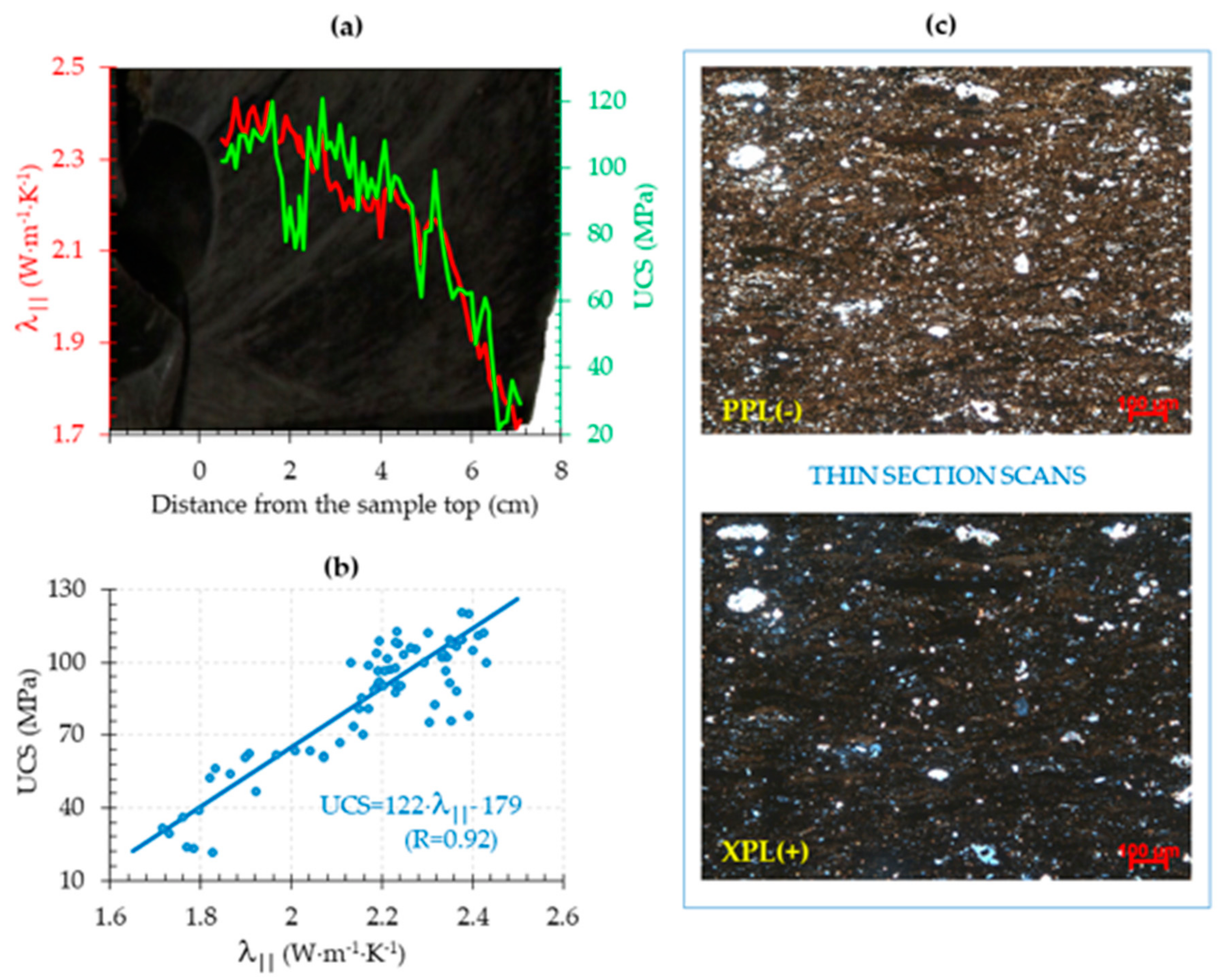
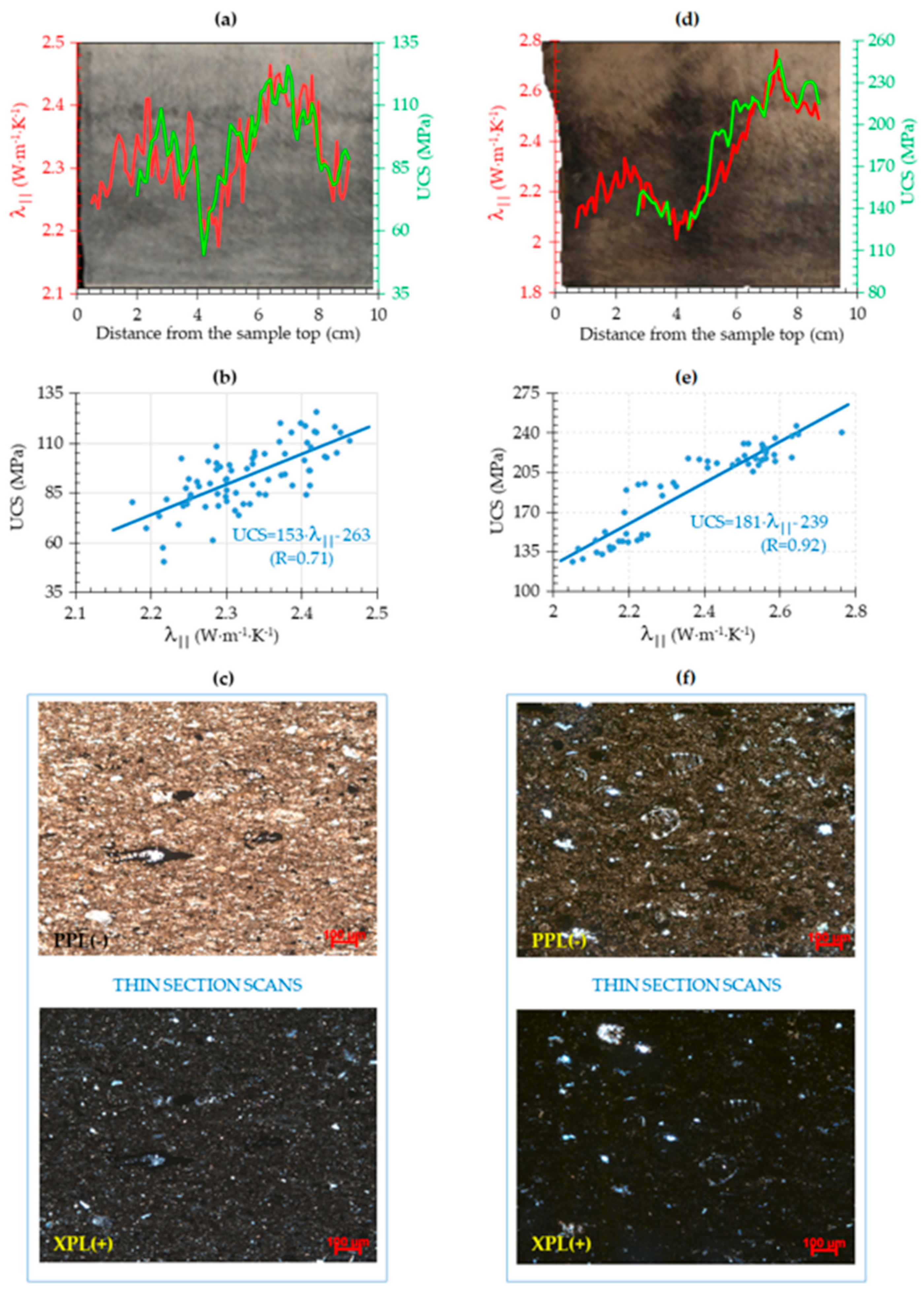
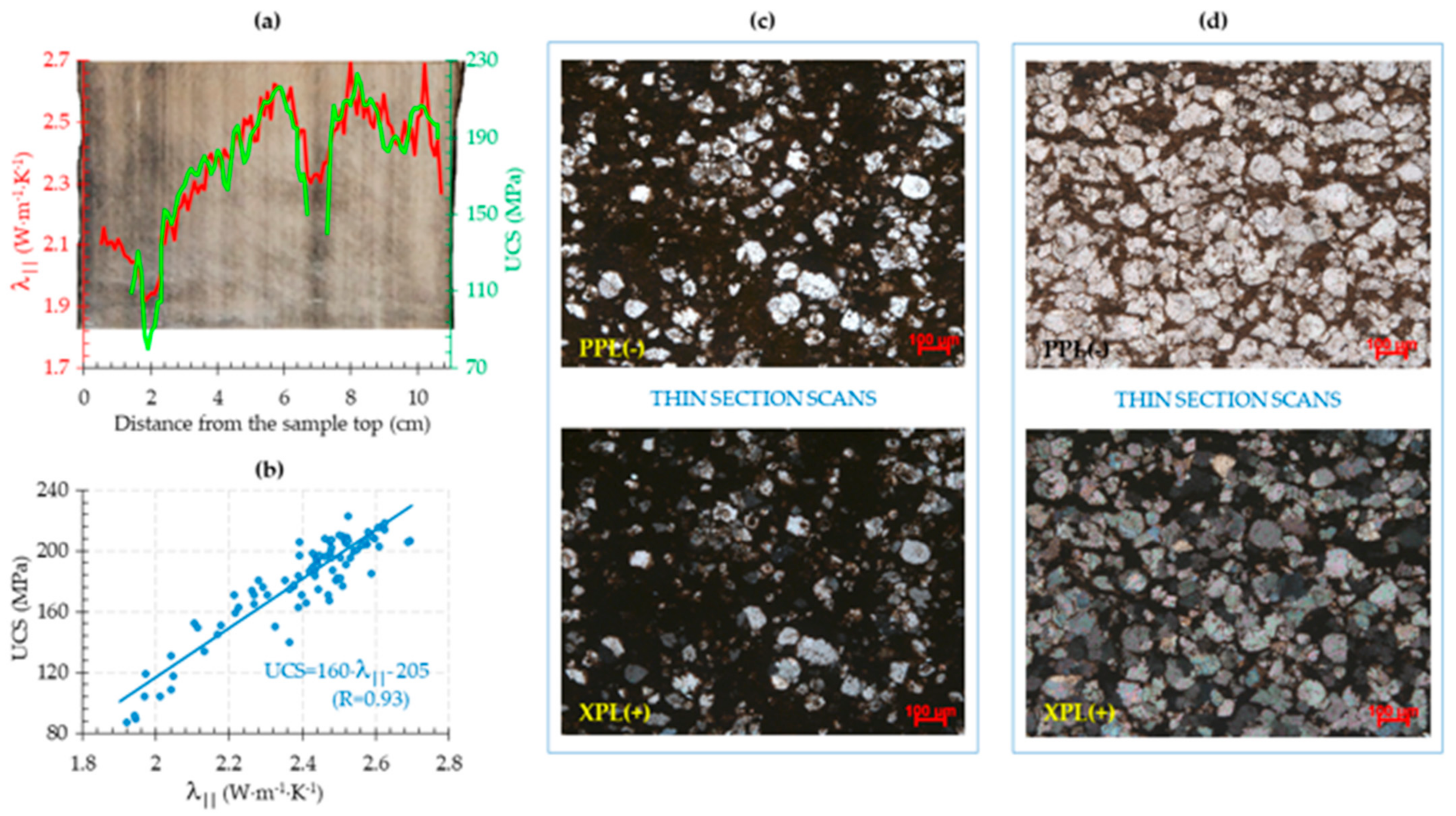
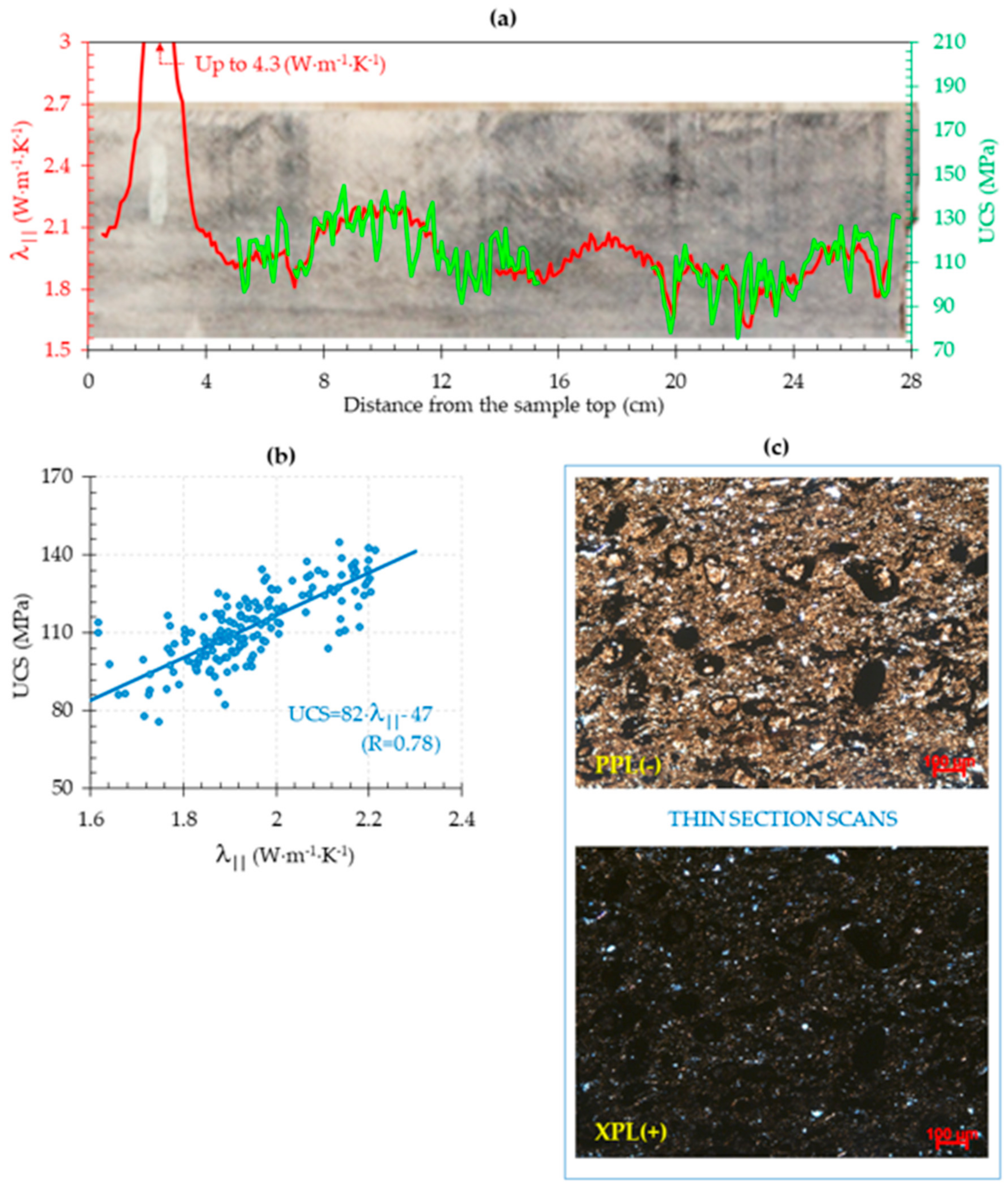
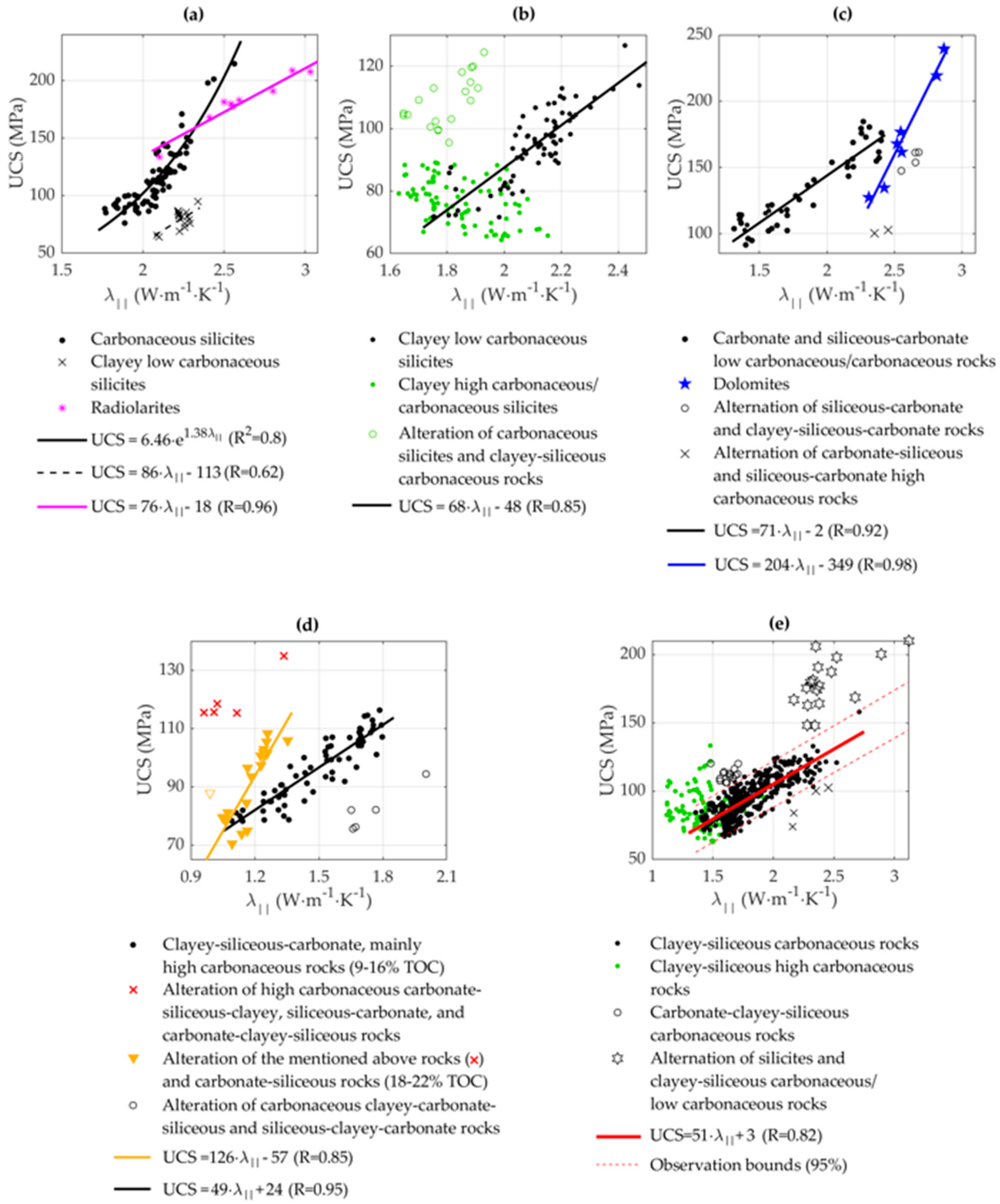
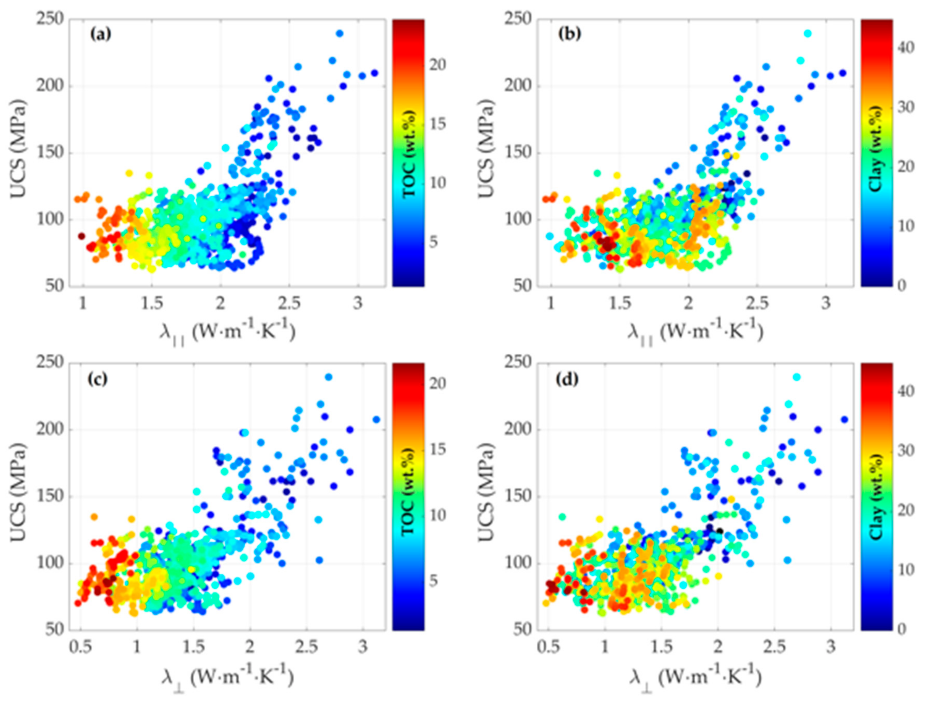
3.2. Comparison of UCS and Thermal Conductivity Profiles

Figure 4, Figure 5, Figure 6, Figure 7, Figure 8 and Figure 9 illustrate the following results for individual samples:
  • The results of comparing the profiles of thermal conductivity (λ||, red curve) and unconfined compressive strength (UCS, green curve) placed on the photograph of the flat surface of the major part of the core sample after slabbing.
  • Scatter plot showing the relationship of thermal conductivity–UCS with the regression curve, regression equation, and correlation coefficient (R). We excluded single data points that did not lie within the 95% confidence interval when finding the dependencies.
  • Thin section scans under plane-polarized light (PPL or uncrossed nicols) and crossed polars (XPL or crossed nicols).
The significance of the established regression equations and the correlation coefficient (Figure 4, Figure 5, Figure 6, Figure 7, Figure 8 and Figure 9) was checked using the Student’s test. This showed that the established regression equations are significant, with a probability of 95%.
Table 2 shows the available data on the material composition obtained from the results of the petrographic description of thin sections (taking into account the results of pyrolysis).

3.3. Comparison of Upscaled UCS and Thermal Conductivity Data

The relationships between unconfined compressive strength and thermal conductivity components λ|| and λ for different lithophysical types (see details in Table 1 and Figure 2) after upscaling with a 30 cm moving average filter are presented in Figure 10, where every point reflects the data over the 30 cm interval.
Three groups were detected using a crossplot for the lithophysical type 1 (Figure 10a): mainly carbonaceous silicites (black dots, representative sample #719, Figure 5d–f), radiolarites (magenta asterisk, representative samples #91–92, Figure 8d–f), and clayey low carbonaceous silicites (black crosses). The last group with decreased UCS values represents rocks from the interval xx80.5–xx81.7 m in well A—i.e., just from the boundary of two lithophysical types. A representative sample of this group, sample #888, is shown in Figure 5a–c. The rock typization was complicated here by the high heterogeneity of the formation and insufficient spatial resolution of the logging data.
Three groups can be selected for lithophysical type 2 (Figure 10b) accounting for TOC data: clayey low carbonaceous silicites (i.e., the group with TOC < 5%, black dots), clayey high carbonaceous/carbonaceous silicites (green dots), and the alteration of carbonaceous silicites and clayey-siliceous carbonaceous rocks (green circles, representative samples #815–816, Figure 9).
Four groups are observed on the crossplot corresponding to the lithophysical type 3 (Figure 10c): carbonate and siliceous-carbonate low carbonaceous/carbonaceous rocks (black dots), dolomites (blue stars), the alternation of siliceous-carbonate and clayey-siliceous-carbonate rocks (black circles, representative samples #118, Figure 6), and the alternation of carbonate-siliceous and siliceous-carbonate high carbonaceous rocks (black crosses, representative samples #35, Figure 4).
Four groups were observed on the crossplot with data on lithophysical type 4 (Figure 10d): clayey-siliceous-carbonate, mainly highly carbonaceous rocks (black dots, 9–16% TOC), as well as three groups (marked by red crosses, orange triangles, and black circles) corresponding to different alteration intervals. Red crosses correspond to the rocks from intervals of the alteration of highly carbonaceous (16–18% TOC) rocks: carbonate-siliceous-clayey, siliceous-carbonate, and carbonate-clayey-siliceous rocks. Orange triangles correspond to highly carbonaceous rocks (18–22% TOC), including the same “mixture” as the group above plus carbonate-siliceous rocks. Black circles correspond to carbonaceous rocks (9–10% TOC) represented by the alteration of clayey-carbonate-siliceous and siliceous-clayey-carbonate rocks.
The analysis of the crossplot on the lithophysical type 5 (Figure 10e) was performed using TOC data. The data corresponding to the highly carbonaceous rocks does not demonstrate any “thermal conductivity-UCS” dependence in contrast to carbonaceous rocks. In the regression analysis of the carbonaceous group, some of the data fall outside the 95% confidence interval (shown by the red dotted line in Figure 10f), forming two subgroups. Hexagrams correspond to the alternation of silicites and clayey-siliceous carbonaceous/low carbonaceous rocks, while black circles correspond to carbonate-clayey-siliceous rocks.
Note that the established regression equations are also statistically significant with a probability of 95%. Many of the indicated groups cannot be distinguished only by the results of the analysis of the UCS profile or by only analyzing the thermal conductivity profile.

4. Discussion

4.1. Heterogeneity and Anisotropy

The results for the detailed profile studies of the rocks of the Bazhenov Formation (Figure 2 and Figure 3) showed the high heterogeneity of the rocks in terms of UCS and thermal conductivity, both within one sample and along the section, which is typical for shales [3]. The first reason for this is their composition, particularly the presence of low-conductive (in comparison with the thermal conductivity of the mineral matrix), relatively compliant, porous organic matter. UCS is also strongly dependent on the presence of another relatively compliant phase: clay minerals. In contrast, the thermal conductivity of clays does not differ much from the thermal conductivity of other minerals found in the Bazhenov Formation, except for pyrite (thermal conductivity is 41.4 W·m−1·K−1) and dolomite (5.7–6.3 W·m−1·K−1) [28]. For example, a slight decrease in the siliceous mineral content and a significant increase in the clay mineral content (sample #888 compared to #719, Figure 5) leads to a decrease in UCS by approximately two and a half times, despite the lower organic matter content in sample #888. At the same time, the average values of the thermal conductivity of samples #719 and #888 differ insignificantly, and the range of changes in thermal conductivity in sample #719 is much broader than that in sample #888 (due to the both increased siliceous component and broader variation in the organic matter content).
According to Zoback and Kohli [2], both organic matter and clay in the rock matrix significantly impact the mechanical (and flow) properties. In our case, the UCS generally decreased with an increasing clay plus TOC content, which is in agreement with published reports on rock behavior [2]. Distinguishing the independent effects of clay and kerogen on physical properties (particularly UCS) is very difficult. At the same time, thermal conductivity is more sensitive to a change in the content of organic matter than to a change in the content of clays (this follows from the comparison of the crossplot coloring in Figure 11a,b or Figure 11c,d). This feature can be used to distinguish the independent effects of clay and kerogen.
Moreover, in addition to the organic matter content, the features of its spatial distribution are essential (as it affects the anisotropy of all transport properties). The features can be seen on thin sections of samples #719, #96–97, and #815–816. Here TOC is about 9% (Table 2), while kerogen is distributed in the rock in the form of irregular lenticular inclusions directed along the bedding (Figure 4c), or thin layers (Figure 8c), or uniformly distributed inclusions—globules (Figure 9c). The black color on these figures corresponds to the kerogen (and pyrite, which developed mainly on the organic substrate). However, the determination of the anisotropy of elastic strength properties is a complex, time-consuming process. By contrast, the determination of the anisotropy of thermal conductivity, which is closely linked with Thomsen’s parameters ε and γ in the Bazhenov Formation [14], is easy to implement in practice using the optical scanning technique.
The comparison plots in Figure 12a,b show that the relationships between the thermal anisotropy coefficient and thermal conductivity perpendicular to the bedding are individual for different TOC ranges. This cannot be explained by a variation in the content of clay minerals, but it can be explained by the features of the spatial distribution of organic matter. Kerogen accumulations are distributed in the rock matrix (of the studied deposits of the Bazhenov Formation) either uniformly or in the form of spots and layered-plane horizontal-lenticular fibers [14]. Other possible reasons for this behavior are a variation in porosity or a relatively high degree of spatial heterogeneity in the void space of the Bazhenov Formation [24] (see Section 4.2).
The significant vertical spatial heterogeneity (and anisotropy in thermal conductivity) of almost every core sample of the Bazhenov Formation means that a proper selection of samples for any laboratory studies requires taking into account the results of high-resolution profile studies.

4.2. Relationships between UCS and Thermal Conductivity

The results obtained (Figure 4, Figure 5, Figure 6, Figure 7, Figure 8 and Figure 9) show that an increase in thermal conductivity with increasing UCS is observed in most cases. The found correlations were primarily driven by the presence of organic matter in the formation and porosity variation due to the contrast between the properties of the rock mineral matrix and kerogen or pore fluid. UCS, as a rule, decreases with an increasing TOC [29,30], as kerogen is a less stiff constituent in rocks (see the comparison of rock-forming minerals in [31]). In carbonaceous silicites and clayey silicites of the studied rocks, an inverse relationship was established between the amount of organic matter and the siliceous component. This means that an increase in the silicon content is accompanied by a decrease in the organic matter content and, consequently, by an increase in UCS (as in the siliceous mudrocks from the Wolfcamp/Leonard strata, Midland Basin, Texas [32]). The thermal conductivity decreases with increasing TOC [33], as the thermal conductivity of organic matter is more than ten times lower than the thermal conductivity of the mineral matrix [12].
At the same time, the dependence established—for example, for sample #118 (Figure 6)—cannot be explained by TOC variation, since the TOC content does not exceed 3.5%. Therefore, other possible reasons for the relationship are a variation in porosity or a relatively high degree of spatial heterogeneity in the void space of the Bazhenov Formation (see [24] and references therein). Porosity affects both the thermal conductivity and UCS (see details in Section 4.2). Higher-porosity domains in a material are usually weaker and less conductive than low-porosity zones. Therefore, it is not surprising that there are approaches to transform the UCS profile [9] or the thermal conductivity profile [12] into a porosity profile for fixed lithology. However, porosity cannot easily and unambiguously be determined from either core or log data in organic shales [34]. Moreover, it is impossible to assess the individual influence of porosity (i.e., without the influence of kerogen) on the UCS–thermal conductivity relationship without measuring the thermal conductivity, UCS, and porosity in the same sample.
There is no unique relationship between thermal conductivity and UCS (Figure 10) for several reasons. First, although these properties are influenced by practically the same factors—the mineral composition and organic matter content, porosity, fluid saturation, textural features, etc.—it can affect thermal conductivity and UCS in many ways. For example, the UCS of a dry sample will exceed that of a sample when saturated [1,35], while the thermal conductivity of a dry sample will be below that when saturated by oil, water, or its mixture (thermal conductivity is about 0.58–0.6 W·m−1·K−1 for water, 0.10–0.18 W·m−1·K−1 for oil/kerosene, 1.3–7.6 W·m−1·K−1 for mineral matrix [12]). Water-wet samples are often weaker than kerosene-wet samples [33], while the thermal conductivity of water-wet samples is higher than that of kerosene-wet samples (kerosene is used as a thermal oil model in experiments because of its similarity in thermal properties). Moreover, it is known that the salinity of the formation water does not significantly affect the thermal conductivity of the saturated rock [36], while some experts note the effect of salinity on stress–strain curves and the UCS [37]. Increasing the clay content decreases the UCS for clay-bearing rocks [38], while it can both decrease and increase (for clayey sandstones) the thermal conductivity. For the studied Bazhenov Formation rocks, increasing the clay content slightly decreased both the thermal conductivity and the UCS, with a high dispersion.
Secondly, rock-forming minerals can be contrasting in one property and non-contrasting in another property. As a result, different rocks may have the same thermal conductivity values at different UCSs or the same UCS values at different thermal conductivities. Unfortunately, reliable information on the UCS of rock constituents is absent, while the published ranges of UCS for common rock types overlap strongly [39,40]. For example, according to Fjaer et al. [40], the UCS varies from 40 to 350 MPa in dolomites and from 2 to 250 MPa in shales. The anisotropy and nonadditivity of UCS and thermal conductivity further complicate joint analysis.
Local discrepancies between the UCS and thermal conductivity profiles of individual samples (Figure 3, Figure 4, Figure 5, Figure 6, Figure 7 and Figure 8) can also be explained by the following factors:
  • The high heterogeneity of specimens and profiling in different areas of the same specimen or its parts (see Figure 1);
  • A change in the core state caused by both the disintegration of samples (due to scratching, drilling plugs, and transporting core samples after scratching back to core storage) and the time lag between the scratch test and optical scanning (i.e., by drying cores over time).
Despite the above features, the integration of scratching data and thermal profiling is of practical interest, particularly for unconventional formations [10,12,14,17,20,41,42,43,44], since it allows us to refine the rock typing, quantitatively evaluate heterogeneity in strength and thermal properties, determine the locations of sampling for further laboratory studies (accounting for rock heterogeneity and thermal anisotropy), and establish for individual intervals the dependence of the “UCS–thermal conductivity” relationship to further use them for predicting UCS with the results of optical scanning.

4.3. Lessons Learned and Future Research Directions

For future studies, we firstly recommend carrying out thermophysical profiling on samples prepared for scratch tests along the lines where scratching will be performed. A corresponding optical scanning unit mounted on a scraper was developed and described in [9,17,33,35]. Joint profiling provides many benefits:
  • It excludes the problem of the relative positioning of rock samples during different types of profiling and automatically adjusts the thermal conductivity and UCS profiles for depth.
  • It excludes the effect of the partial or complete destruction of samples of weakly consolidated and/or fractured rocks due to core transfer from the geomechanical lab back to core storage and the repeated stacking of rock samples on the tool and returning them to the boxes in which the rock samples are stored.
  • It eliminates the influence of differences in the saturation on the profiling results of various properties (as the saturation of the samples during scratching and thermophysical profiling will be the same).
  • It excludes the influence of possible horizontal spatial heterogeneity on the results of the profiling of various properties (scratching will be carried out along the same line/sections of the samples as thermal profiling).
  • It significantly increases the performance of measurements.
  • It can allow us to control the partial sample disintegration caused by the mechanical impact of the cutter on the sample (by comparing the results of thermal profiling obtained before the first iteration of scratching and after the scratch test).
Secondly, it is necessary to estimate the total uncertainty (combination of systematic and random errors) in UCS measurements and develop a procedure for excluding those data from the UCS profile that corresponds to UCS variations caused by edge effects (scratching near the sample boundaries) or sample disintegration during the scratch test.
Thirdly, it is not necessary to scratch the entire core column, thereby preventing core disintegration and saving core samples for other studies. Preliminary results of non-destructive thermal profiling, along with the macro description of cores, will make it possible to determine individual representative intervals for the scratch test. If the dependency of UCS–thermal conductivity is established, UCS profiles could be obtained based only on the thermal conductivity profiles.
UCS and thermal conductivity (as well as the volumetric heat capacity or thermal diffusivity of rocks measured simultaneously with thermal conductivity using optical scanning, which were not considered in this study) are data of different physical natures. The large volume of these data obtained with a high resolution of ~ 1 mm creates the need to use machine learning methods to express the processing and analysis of the profiling results (see, for example, [4,7,44]).

5. Conclusions

High-resolution scratch testing and non-destructive thermal core profiling performed on 1061 samples from the Bazhenov Formation allowed us to quantify the formation heterogeneity at different scales (from mm to meters) for two physical properties –UCS and thermal conductivity–and carry out the joint analysis.
The analysis allowed us to make the following conclusions:
  • A positive correlation between thermal conductivity and UCS is often observed. Established relationships are primarily driven by the presence/distribution of organic matter in a formation.
  • Correlations are unique to the different rock types found in the formation and may be used to predict UCS without the core surface destruction or core foliation that is typical for the scratch testing of shales.
  • Thermal conductivity is more sensitive to a change in the content of organic matter than to a change in the content of clays (in opposite to UCS) that can be used to distinguish the independent effects of clay and kerogen.
  • The analysis of crossplots of UCS and thermal conductivity helps one to observe heterogeneities and facies that would be difficult or impossible to see using logging data analysis or geological description alone. This will contribute to the sampling strategy for unconventional reservoirs for future laboratory investigations of core samples.
The integration of thermal core profiling and scratch testing data looks promising for un-conventional reservoir characterization (especially if the pitfalls described in this paper will be accounted for when organizing future measurements and research).

Author Contributions

Conceptualization, E.C. and Y.P.; methodology, E.C., Y.P. and E.P.; software, E.C.; validation, Y.P., R.R. and E.P.; formal analysis, E.C. and R.R.; investigation, E.C., Y.P., R.R. and E.P.; resources, V.Z.; data curation, D.Z.; writing—original draft preparation, E.C. and Y.P.; writing—review and editing, R.R., E.P., D.Z. and V.Z.; supervision, Y.P. and D.Z.; project administration, V.Z. All authors have read and agreed to the published version of the manuscript.

Funding

This work was supported by the Ministry of Science and Higher Education of the Russian Federation under agreement No. 075–10−2020–119 within the framework of the development program for a world-class research center.

Institutional Review Board Statement

Not applicable.

Informed Consent Statement

Not applicable.

Data Availability Statement

Restrictions apply to the availability of these data. Data were obtained from LLC Gazpromneft Scientific and Technical Center and are available from the corresponding author with the permission of LLC Gazpromneft Scientific and Technical Center.

Acknowledgments

Authors thank Mikhail Yu. Spasennykh from Skolkovo Institute of Science and Technology for funding acquisition, Georgy A. Kalmykov and Anton G. Kalmykov from Moscow State University for the macro description of cores, Olga V. Postnikova and Alexander V. Postnikov from Gubkin University for the petrographic analysis of thin sections, and our colleague Egor G. Savelyev from Skolkovo Institute of Science and Technology for his assistance in conducting thermal profiling. The authors also thank two anonymous Reviewers and Academic Editor for their careful reading and valuable recommendations that resulted in the increasing quality of the manuscript.

Conflicts of Interest

The authors declare no conflict of interest.

References

  1. McPhee, C.; Reed, J.; Zubizarreta, I. Core Analysis: A Best Practice Guide. Developments in Petroleum Science, Volume 64; Elsevier: Amsterdam, The Netherlands, 2015. [Google Scholar] [CrossRef]
  2. Zoback, M.D.; Kohli, A.H. Unconventional Reservoir Geomechanics; Cambridge University Press: New York, NY, USA, 2019. [Google Scholar] [CrossRef]
  3. Jin, Z.; Li, W.; Jin, C.; Hambleton, J.; Cusatis, G. Anisotropic elastic, strength, and fracture properties of Marcellus shale. Int. J. Rock Mech. Min. Sci. 2018, 109, 124–137. [Google Scholar] [CrossRef] [Green Version]
  4. Cook, J.; Frederiksen, R.A.; Hasbo, K.; Green, S.; Judzis, A.; Wesley Martin, J.; Suarez-Rivera, R.; Herwanger, J.; Hooyman, P.; Lee, D.; et al. Rocks matter: Ground truth in geomechanics. Oilfield Rev. 2007, 19, 36–55. [Google Scholar]
  5. Lai, J.; Wang, G.; Fan, Z.; Chen, J.; Qin, Z.; Xiao, C.; Wang, S.; Fan, X. Three-dimensional quantitative fracture analysis of tight gas sandstones using industrial computed tomography. Sci. Rep. 2017, 7, 1–12. [Google Scholar] [CrossRef] [PubMed]
  6. Richard, T.; Detournay, E.; Drescher, A.; Nicodeme, P.; Fourmaintraux, D. The scratch test as a means to measure strength of sedimentary rocks. In Proceedings of the SPE/ISRM Rock Mechanics in Petroleum Engineering, Trondheim, Norway, 8–10 July 1998. Paper Number SPE-47196-MS. [Google Scholar] [CrossRef]
  7. Suarez-Rivera, R.; Ostroff, G.; Tan, K.; Begnaud, B.; Martin, W.; Bermudez, T. Continuous rock strength measurements on core and neural network modeling result in significant improvements in log-based rock strength predictions used to optimize completion design and improve prediction of sanding potential and wellbore stability. In Proceedings of the SPE Annual Technical Conference and Exhibition, Denver, CO, USA, 5–8 October 2003. Paper Number SPE-84558-MS. [Google Scholar] [CrossRef]
  8. Richard, T.; Dagrain, F.; Poyol, E.; Detournay, E. Rock strength determination from scratch tests. Eng. Geol. 2012, 147–148, 91–100. [Google Scholar] [CrossRef]
  9. Germay, C.; Richard, T.; Mappanyompa, E.; Lindsay, C.; Kitching, D.; Khaksar, A. The continuous-scratch profile: A high-resolution strength log for geomechanical and petrophysical characterization of rocks. SPE Res. Eval. Eng. 2015, 18, 432–440. [Google Scholar] [CrossRef]
  10. Popov, Y.; Parshin, A.; Chekhonin, E.; Gorobtsov, D.; Miklashevskiy, D.; Korobkov, D.; Suarez-Rivera, R.; Green, S. Rock heterogeneity from thermal profiles using an optical scanning technique. In Proceedings of the 46th US Rock Mechanics/Geomechanics Symposium, Chicago, IL, USA, 24–27 June 2012. Paper Number ARMA-2012-509. [Google Scholar]
  11. Popov, Y.; Beardsmore, G.; Clauser, C.; Roy, S. ISRM Suggested methods for determining thermal properties of rocks from laboratory tests at atmospheric pressure. Rock Mech. Rock Eng. 2016, 49, 4179–4207. [Google Scholar] [CrossRef]
  12. Popov, E.; Popov, Y.; Chekhonin, E.; Safonov, S.; Savelev, E.; Gurbatova, I.; Ursegov, S.; Shakirov, A. Thermal core profiling as a novel and accurate method for efficient characterization of oil reservoirs. J. Petrol. Sci. Eng. 2020, 193, 107384. [Google Scholar] [CrossRef]
  13. TerraTek Services—Mechanical Property Profiling. Product Sheet 13-TS-0143. 2014 Schlumberger. Available online: https://www.slb.com/-/media/files/testing-services/product-sheet/terratek-mp2-mechanical-properties-ps.ashx (accessed on 14 May 2021).
  14. Chekhonin, E.; Popov, E.; Popov, Y.; Gabova, A.; Romushkevich, R.; Spasennykh, M.; Zagranovskaya, D. High-resolution evaluation of elastic properties and anisotropy of unconventional reservoir rocks via thermal core logging. Rock Mech. Rock Eng. 2018, 51, 2747–2759. [Google Scholar] [CrossRef]
  15. Chang, C.; Zoback, M.D.; Khaksar, A. Empirical relations between rock strength and physical properties in sedimentary rocks. J. Petrol. Sci. Eng. 2006, 51, 223–237. [Google Scholar] [CrossRef]
  16. Hareland, G.; Nygård, R. Calculating unconfined rock strength from drilling data. In Proceedings of the 1st Canada-US Rock Mechanics Symposium, Vancouver, BC, Canada, 27–31 May 2007; Available online: https://www.rocsoltech.com/wp-content/uploads/2018/09/Calculating-Unconfined-Rock-Strength-From-Drilling-Data.pdf (accessed on 14 May 2021).
  17. Popov, Y.; Parshin, A.; Chekhonin, E.; Popov, E.; Miklashevskiy, D.; Suarez-Rivera, R.; Green, S. Continuous core thermal properties measurements and analysis. In Proceedings of the 47th US Rock Mechanics/Geomechanics Symposium, San Francisco, CA, USA, 23–26 June 2013. Paper Number ARMA-13391. [Google Scholar]
  18. Yasar, E.; Erdogan, Y.; Guneyli, H. Determination of the thermal conductivity from physico-mechanical properties. Bull. Eng. Geol. Environ. 2008, 67, 219–225. [Google Scholar] [CrossRef]
  19. Khaksar, A.; Taylor, P.G.; Fang, Z.; Kayes, T.J.; Salazar, A.; Rahman, K. Rock strength from core and logs, where we stand and ways to go. In Proceedings of the EUROPEC/EAGE Conference and Exhibition, Amsterdam, The Netherlands, 8–11 June 2009. [Google Scholar] [CrossRef]
  20. Chekhonin, E.M.; Gabova, A.V.; Popov, E.Y.; Ovcharenko, Y.V.; Popov, Y.A. New approach for evaluation of geomechanical parameters of low-permeable anisotropic rocks. In Proceedings of the 2018 European Rock Mechanics Symposium “Geomechanics and Geodynamics of Rock Masses”, Saint Petersburg, Russia, 22–26 May 2018; CRC Press: London, UK, 2018; Volume 2, pp. 1351–1356. [Google Scholar] [CrossRef]
  21. Technically Recoverable Shale Oil and Shale Gas Resources: An Assessment of 137 Shale Formations in 41 Countries outside the United States. US Energy Information Administration (EIA), June 2013. Available online: https://www.eia.gov/analysis/studies/worldshalegas/pdf/overview.pdf (accessed on 14 May 2021).
  22. Ulmishek, G.F. Petroleum Geology and Resources of the West Siberian Basin, Russia. US Geological Survey Bulletin 2201-G. US Geological Survey, Reston, Virginia, 2003. Available online: https://pubs.usgs.gov/bul/2201/G/B2201-G.pdf (accessed on 14 May 2021).
  23. Gurari, F.G.; Vaits, E.Y.; Melenevskii, V.N.; Moskvin, V.I.; Perozio, G.N.; Predtechenskaya, E.A.; Rudnitskaya, D.I.; Stasova, O.F.; Frolov, V.K.; Frolova, L.A. Formation Conditions and Prospecting for Oil Accumulations in Mudstones of the Bazhenov Formation; Nedra: Moscow, Russia, 1988. (In Russian) [Google Scholar]
  24. Kalmykov, G.A.; Balushkina, N.S. A Model of Oil Saturation in the Pore Space of the Rocks of the Bazhenov Formation in Western Siberia and Its Use for Assessing the Resource Potential; GEOS: Moscow, Russia, 2017; (In Russian). ISBN 978-5-89118-763-4. [Google Scholar]
  25. Gavrilov, A.E.; Zhukovskaya, E.A.; Tugarova, M.A.; Ostapchuk, M.A. Objective Bazhenov rocks classification (the case of the West Siberia central part fields). Neftyanoe Khozyaystvo—Oil Ind. 2015, 12, 38–40. [Google Scholar]
  26. Litho Scanner: High-Definition Spectroscopy Service. Brochure 17-FE-259463. Schlumberger. 2017. Available online: https://www.slb.com/-/media/files/fe/brochure/litho-scanner-br.ashx (accessed on 14 May 2021).
  27. Scott, D.W. On optimal and data-based histograms. Biometrika 1979, 66, 605–610. [Google Scholar] [CrossRef]
  28. Popov, Y.A.; Berezin, V.V.; Soloviov, G.A.; Romuschkevitch, R.A.; Korosteliov, V.M.; Kostiurin, A.A.; Kulikov, A.V. Thermal conductivity of minerals. Izv. Phys. Solid Earth 1987, 23, 245–253. [Google Scholar]
  29. Eseme, E.; Urai, J.L.; Krooss, B.M.; Littke, R. Review of mechanical properties of oil shales: Implications for exploitation and basin modelling. Oil Shale 2007, 24, 159–174. Available online: https://www.kirj.ee/public/oilshale/oil-2007-2-7.pdf (accessed on 14 May 2021).
  30. Dradjat, A.S.; Djamil, A.; Aprizal, M. Seismic anisotropy VTI modeling and mechanical properties of kerogen in gas shale. In Proceedings of the AAPG Asia Pacific Region GTW, The Art of Hydrocarbon Prediction: Managing Uncertainties Technical Symposium, Bogor, Indonesia, 7–8 August 2019. Article 42486. [Google Scholar] [CrossRef]
  31. Khatibi, S. Fine Scale Characterization of Organic Matter Using Analytical Methods: Raman and NMR Spectroscopies. Ph.D. Thesis, University of North Dakota, Grand Forks, ND, USA, 2019. Available online: https://commons.und.edu/theses/2566 (accessed on 14 May 2021).
  32. Baumgardner, R.W., Jr.; Hamlin, H.S.; Rowe, H.D. High-resolution core studies of Wolfcamp/Leonard basinal facies, Southern Midland Basin, Texas. In Proceedings of the AAPG Southwest Section Annual Convention, Midland, TX, USA, 11–14 May 2014; Article #10607. Available online: http://www.searchanddiscovery.com/documents/2014/10607baumgardner/ndx_baumgardner.pdf (accessed on 14 May 2021).
  33. Popov, E.Y. Development of an Experimental Base of Thermal Petrophysics for Studying Rocks of Fields with Hard-to-Recover and Unconventional Hydrocarbon Reserves. Ph.D. Thesis, Schmidt Institute of Physics of the Earth of the Russian Academy of Sciences, Moscow, Russia, 2020. (In Russian). [Google Scholar]
  34. Vernik, L.; Milovac, J. Rock physics of organic shales. Lead. Edge 2011, 30, 318–323. [Google Scholar] [CrossRef]
  35. Al-Bazali, T. The impact of water content and ionic diffusion on the uniaxial compressive strength of shale. Egypt. J. Petrol. 2013, 22, 249–260. [Google Scholar] [CrossRef] [Green Version]
  36. Chekhonin, E.; Parshin, A.; Pissarenko, D.; Popov, Y.; Romushkevich, R.; Safonov, S.; Spasennykh, M.; Chertenkov, M.; Stenin, V. When rocks get hot: Thermal properties of reservoir rocks. Oilfield Rev. 2012, 24, 20–37. Available online: https://www.slb.com/-/media/files/oilfield-review/2-rocks-hot-2-english (accessed on 14 May 2021).
  37. Suo, Y.; Chen, Z.; Rahman, S.S.; Chen, X. Experimental study on mechanical and anisotropic properties of shale and estimation of uniaxial compressive strength. Energy Sour. Part A Recov. Util. Environ. Eff. 2020, 1. [Google Scholar] [CrossRef]
  38. Kahraman, S.; Aloglu, A.S.; Saygin, E.; Aydin, B. The effect of clay content on the relation between uniaxial compressive strength and needle penetration index for clay-bearing rocks. Int. J. Geo-Eng. 2021, 12, 6. [Google Scholar] [CrossRef]
  39. Schon, J.H. Physical Properties of Rocks: A Workbook; Elsevier: Amsterdam, The Netherlands, 2011; ISBN 978-0-444-53796-6. [Google Scholar]
  40. Fjaer, E.; Holt, R.M.; Horsrud, P.; Raane, A.M.; Risnes, R. Petroleum Related Rock Mechanics, 2nd ed.; Elsevier Science: Amsterdam, The Netherlands, 2008; Volume 53, ISBN 978-0-444-50260-5. [Google Scholar]
  41. Popov, Y.A.; Popov, E.Y.; Chekhonin, E.M.; Gabova, A.V.; Romushkevich, R.A.; Spasennykh, M.Y.; Zagranovskaya, D.E. Investigation of Bazhenov formation using thermal core logging technique. Neftyanoe Khozyaystvo—Oil Ind. 2017, 3, 22–27. [Google Scholar] [CrossRef]
  42. Chekhonin, E.; Shakirov, A.; Popov, E.; Romushkevich, R.; Popov, Y.; Bogdanovich, N.; Rudakovskaya, S. The role of thermophysical profiling for core sampling for laboratory investigations of source rocks. In Proceedings of the EAGE/SPE Workshop on Shale Science: Theory and Practice, Moscow, Russia, 8–9 April 2019. [Google Scholar] [CrossRef]
  43. Chekhonin, E.; Popov, E.; Popov, Y.; Romushkevich, R.; Savelev, E.; Shakirov, A. Thermal petrophysics: New insight into core analysis and characterization of highly heterogeneous tight oil formations. In Proceedings of the 80th EAGE Conference and Exhibition, Copenhagen, Denmark, 11–14 June 2018. [Google Scholar] [CrossRef]
  44. Meshalkin, Y.; Koroteev, D.; Popov, E.; Chekhonin, E.; Popov, Y. Robotized petrophysics: Machine learning and thermal profiling for automated mapping of lithotypes in unconventionals. J. Petrol. Sci. Eng. 2018, 167, 944–948. [Google Scholar] [CrossRef]
Figure 1. Schemes of (a) the full-diameter sample orientation and position with respect to the bedding plane; (b) the slabbed sample (with the vertical scratch groove) comes apart in three pieces during scratching at the geomechanical lab; (c) pieces of the samples after plug drilling (black hole in the major slab in the center) with the direction and location of optical scanning (red dashed lines) performed in core storage. Example of one and a half clayey-siliceous samples with (d) UCS and thermal conductivity profiles after adjusting for depth; (e) UCS profiles placed on a photo of the flat core surface made before the scratch test (green arrows show the boundaries of the samples); (f) thermal conductivity placed on a photo of the samples disintegrated after the scratch test (red arrows indicate new boundaries between pieces; samples that were too short were not profiled with the optical scanner).
Geosciences 11 00260 g001
Figure 2. Profiles of thermal conductivity components and unconfined compressive strength at different scales along three wells drilled through the Bazhenov Formation: (a) wellbore A, (b) wellbore B (where the upper part of the formation was not cored), (c) wellbore C. Columns with lithophysical rock types are shown on the left side for every well.
Geosciences 11 00260 g002
Figure 3. Histograms for some characteristics of the Bazhenov Formation core samples: (a) the thermal conductivity parallel to bedding, (b) the unconfined compressive strength, (c) the thermal heterogeneity factor of the slabbed core samples studied with the optical scanner, (d) sample lengths of cores studied with the optical scanner.
Geosciences 11 00260 g003
Figure 4. (a) Thermal conductivity and UCS profiles placed on a photo of clayey-carbonate-siliceous high carbonaceous rock (sample #35 from the depth xx23.32 m, well B); (b) results of regression analysis; (c) thin-section scans under plane-polarized light (PPL) and crossed polars (XPL).
Geosciences 11 00260 g004
Figure 5. (a) Thermal conductivity and UCS profiles placed on a photo of low carbonaceous clayey silicite (sample #888 from the depth xx81.43 m, well A; it is recognized as a silicite according to lithophysical typization due to the high heterogeneity of the formation and the insufficient spatial resolution of the logging data); (b) results of the regression analysis for sample #888; (c) thin-section scans under plane-polarized light (PPL) and crossed polars (XPL) for the rocks of sample #888. (d) Thermal conductivity and UCS profiles placed on a photo of carbonaceous silicite (sample #719 from the depth xx67.0 m, well A); (e) results of the regression analysis for sample #719; (f) thin-section scans under plane-polarized light (PPL) and crossed polars (XPL) for the rocks of sample #719.
Geosciences 11 00260 g005
Figure 6. (a) Thermal conductivity and UCS profiles placed on a photo of interval of alternation of siliceous-carbonate and clayey-siliceous-carbonate rocks (sample #118 from the depth xx34.27 m, well B); (b) results of regression analysis; thin-section scans under plane-polarized light (PPL) and crossed polars (XPL) for (c) siliceous-carbonate sections and (d) clayey-siliceous-carbonate sections of the sample.
Geosciences 11 00260 g006
Figure 7. (a) Thermal conductivity and UCS profiles placed on a photo showing the alternation of clayey-carbonate-siliceous carbonaceous and siliceous-carbonate high carbonaceous rocks (sample #796 from the depth xx73.35 m, well A); (b) results of the regression analysis; thin-section scans for (c) clayey-carbonate-siliceous carbonaceous and (d) siliceous-carbonate high carbonaceous sections of the sample.
Geosciences 11 00260 g007
Figure 8. (a) Thermal conductivity and UCS profiles placed on a photo of the interval of alternation of silicites and clayey-siliceous rocks (samples #96–97 from the depth xx31.64 m, well B); (b) results of the regression analysis for samples #96–97; (c) thin-section scans under plane-polarized light (PPL) and crossed polars (XPL) for the rocks of sample #97. (d) Thermal conductivity and UCS profiles placed on a photo of radiolarite (samples #91–92 from the depth xx31.17 m, well B). Here, the optical scanning was carried out along the minor slab because scratching with the following plug drilling resulted in the disintegration of the major slab. (e) Results of the regression analysis for samples #91–92; (f) thin section scans under plane-polarized light (PPL) and crossed polars (XPL) for the rocks of sample #92.
Geosciences 11 00260 g008
Figure 9. (a) Thermal conductivity and UCS profiles placed on a photo of clayey-siliceous, inhomogeneously pyritized, carbonaceous rock (samples #815–816 from the depth xx75.5 m, well A). A local increase in thermal conductivity up to 4.3 W·m−1·K−1 within the interval 2.3 cm from the sample’s top is the result of pyrite inclusion (a light oval spot on the photo). (b) Results of regression analysis; (c) thin-section scans under plane-polarized light (PPL) and crossed polars (XPL).
Geosciences 11 00260 g009
Figure 10. Relationship between unconfined compressive strength and thermal conductivity for different lithophysical types (the type described in Table 1 and Figure 2): (a) low carbonaceous/carbonaceous silicites, (b) clayey low carbonaceous/carbonaceous silicites, (c) carbonate and siliceous-carbonate low carbonaceous/carbonaceous rocks, (d) clayey-siliceous-carbonate high carbonaceous rocks, (e) clayey-siliceous high carbonaceous/carbonaceous rocks. See text for details.
Geosciences 11 00260 g010
Figure 11. Crossplots of unconfined compressive strength and thermal conductivity (a) parallel to bedding with TOC shown in color, (b) parallel to bedding with clay minerals fraction shown in color, (c) perpendicular to bedding with TOC shown in color, (d) perpendicular to bedding with clay minerals fraction shown in color. All studied lithophysical types are presented here; organic and clay content come from the LithoScanner data.
Geosciences 11 00260 g011
Figure 12. Crossplots of thermal anisotropy coefficient and thermal conductivity perpendicular to bedding with (a) TOC shown in color and regression analysis results; (b) clay mineral fraction shown in color.
Geosciences 11 00260 g012
Table 1. Summary of the studied core samples from the Bazhenov Formation.
Lithophysical Type IDBrief DescriptionN of Studied * Core SamplesPercentage to All Studied Cores, %
1Low carbonaceous/carbonaceous silicites14013.2
2Clayey low carbonaceous/carbonaceous silicites20219
3Carbonate and siliceous-carbonate low carbonaceous/carbonaceous rocks615.8
4Clayey-siliceous-carbonate high carbonaceous rocks13212.4
5Clayey-siliceous high carbonaceous/carbonaceous rocks52649.6
* The number of samples in the column is shown for thermal profiling (with a total of 1061 samples); it differs from the number of samples studied by scratching because thermal profiling was performed after the destructive scratch testing when some core samples were split into parts (see details in Section 2.4).
Table 2. Generalized information on rock composition from the results of the petrographic description of thin sections accounting for the results of pyrolysis.
Sample Number, Well IDDescriptionComposition, %
Silica Group MineralsClay MineralsField-SparsCarbonate MineralsPyriteOrganic Matter
#91–92, BSilicite (radiolarite). Skeletal remains of radiolarians 0.08–0.15 mm in size83.07.03.01.01.54.5
#719, ACarbonaceous silicite. Relics of partially carbonated radiolarian shells up to 0.1 mm in diameter74.010.53.01.50.59.0
#96–97, BAlternation of silicites and clayey-siliceous rocks67.812.06.00.74.59.0
#888, ALow carbonaceous clayey silicite61.822.05.03.03.04.5
#815–816, AClayey-siliceous, inhomogeneously pyritized, carbonaceous rock. Relics of pyritized radiolarian shells up to 0.12 mm in diameter52.320.04.03.111.59.0
#796, AClayey-carbonate-siliceous carbonaceous rock44.019.53.522.02.58.5
Siliceous-carbonate high carbonaceous rock with relict biomorphic structure. Relics of radiolarian shells 0.1 mm in diameter replaced by carbonates20.58.06.050.01.514.0
#35, BClayey-carbonate-siliceous high carbonaceous rock. The relics of radiolarian shells are mostly replaced by calcite and dolomite38.016.54.023.56.011.5
#118, BClayey-siliceous-carbonate rock. Relics of radiolarian shells are replaced by calcite and dolomite33.510.53.048.01.53.5
Siliceous-carbonate rock. Relics of radiolarian shells (the content varies from 40% to 80%) up to 0.1 mm in diameter; all shells are replaced by carbonates18.57.02.071.01.50.0
Publisher’s Note: MDPI stays neutral with regard to jurisdictional claims in published maps and institutional affiliations.

