Nonlinear 3D Finite Element Analysis of a Coupled Soil–Structure System by a Deterministic Approach

Abstract

Fully coupled soil–structure analyses were performed for a building of strategic importance located in the city of Messina (Sicily, Italy). The structure was built after the destructive 1908 earthquake, also known as the ‘Messina and Reggio Calabria earthquake’, which caused severe ground shaking. A parametric study considering three seismograms of this earthquake was performed. Deep in situ and laboratory investigations allowed the definition of the geometric and geotechnical model of the subsoil. Numerical analyses were performed with PLAXIS3D finite element software (Version 21.01.00.479). The Hardening Soil model with small-strain stiffness was accurately calibrated using laboratory and field data. The dynamic response was investigated in terms of accelerations, response spectra, amplification functions, displacements and stress–strain hysteretic loops. The findings show that many aspects must be investigated for the retrofitting of buildings with shallow foundation in areas characterized by a medium to high level of seismic risk: (i) a key role is played by an accurate investigation of the soil; taking into account the specific conditions of the soil, it was possible to investigate its filtering effects; (ii) the dynamic response of the fully-coupled soil–structure system deviates from the free field-site response analysis; (iii) the results reveal the importance of considering the soil nonlinearity in seismic soil–structure interaction problems.

1. Introduction

The importance of assessing soil–structure interaction (SSI) effects in the retrofitting and/or improving of an existing structure is recognized by the seismic scientific community [1,2,3]. However, current seismic regulations, such as the Italian seismic code [4], employ a fixed-base assumption, neglecting the SSI effects [2].

The first fundamental aspect of assessing SSI is the analysis of all available geo-physical and dynamic data to define the subsoil model and the geotechnical characterization of the area under study. The geometry and the geophysical and dynamic properties of the superficial layers strongly modify the ground motion in terms of amplitude, duration and wavefield composition [5]. Therefore, for retrofitting and/or improving an existing structure, it is important evaluate the modified ground motion at the surface on which the building is situated; this is the free field (FF) condition [6].

Many recent seismic events, such as the 2009 L’Aquila earthquake, the 2010 Haiti earthquake and the 2016 Norcia earthquake, show the importance of considering the SSI effects for the safeguarding of existing structures or for the planning of new ones [7]. Indeed, the kinematic and inertial interactions between the soil, the foundation and the structure modify the dynamic response at the foundation level [8]. The following two main approaches can be employed to evaluate the SSI effects: the “substructure method” and the “direct method”. In the “substructure method” the soil and the structure are considered separately and then combined. Dashpots and springs are employed to transmit the effect of the interaction between the soil and the foundation to the structure. The “direct method”, adopted in this work, has the advantage of modeling the structure and the soil in a single finite element model (FEM), but it requires considerable calculation efforts [9].

In the FEM, the mechanical behavior of soil is described by means of constitutive material models. Moreover, nonlinear soil behavior can be considered through two kind of analyses: the equivalent linear and nonlinear analyses [10]. Most of the studies on SSI effects employ the equivalent visco-elastic constitutive model, which involves carrying out a series of linear analyses with subsequent updating of the stiffness and damping parameters until a convergence criterion is satisfied [10]. Massimino et al. [8] evaluated the seismic response of a soil–building system by means of the ADINA code using the equivalent visco-elastic constitutive model. Seylabi et al. [11] investigated the capabilities of calibrated equivalent linear models in capturing the dynamic response of buried box structures. Fiamingo et al. [7] performed FEM analyses on a fully coupled soil–structure system for a building damaged during the 26 December 2018 earthquake using an equivalent visco-elastic behavior. However, nonlinear dynamic analysis, which was used in this study, provides a better comprehension of the dynamics of the soil, including its hysteresis. This analysis consists of the step-by-step integration of the equations of motion, simultaneously changing the parameter values of stiffness and damping [10].

An advanced model for the simulation of soil behavior implemented in PLAXIS3D finite element software (Version 21.01.00.479) is the ‘Hardening Soil’ (HS) model [12]. It describes the soil stiffness by using three different input parameters at the reference pressure p^ref: the secant stiffness in a standard drained triaxial test (E₅₀^ref), the unloading/reloading stiffness (E_ur^ref) and the tangent stiffness for primary oedometer loading (E_oed^ref). The HS model also considers the stress-dependency of stiffness moduli. Moreover, the yield surface is not fixed in principal stress space, but it can expand as a result of plastic strain [13,14]. The HS model considers an elastic behavior during unloading and reloading. However, with the increase in strain amplitude, soil stiffness decays nonlinearly. In addition to all characteristics of the HS model, the HS model with small-strain stiffness (HS small model), which was used in this work, includes increased soil stiffness for small strains [15,16].

In this paper, the SSI effects for a strategic building located in the city of Messina (Sicily, Italy) were investigated by means of PLAXIS3D using the HS small model. The study benefits from the availability of ample geophysical survey and laboratory tests. The procedure for the model calibration was accurately delineated. The well-calibrated constitutive model properly describes the stiffness and strength properties of the soil under consideration and accurately captures the soil nonlinearity, allowing an in-depth assessment of the SSI effects. The 1908 Messina and Reggio Calabria earthquake, which was the strongest seismic event of the 20th century in Italy, was considered for the numerical analyses as a scenario earthquake. For this purpose, a parametric study was performed considering three different seismograms related to the 1908 seismic event.

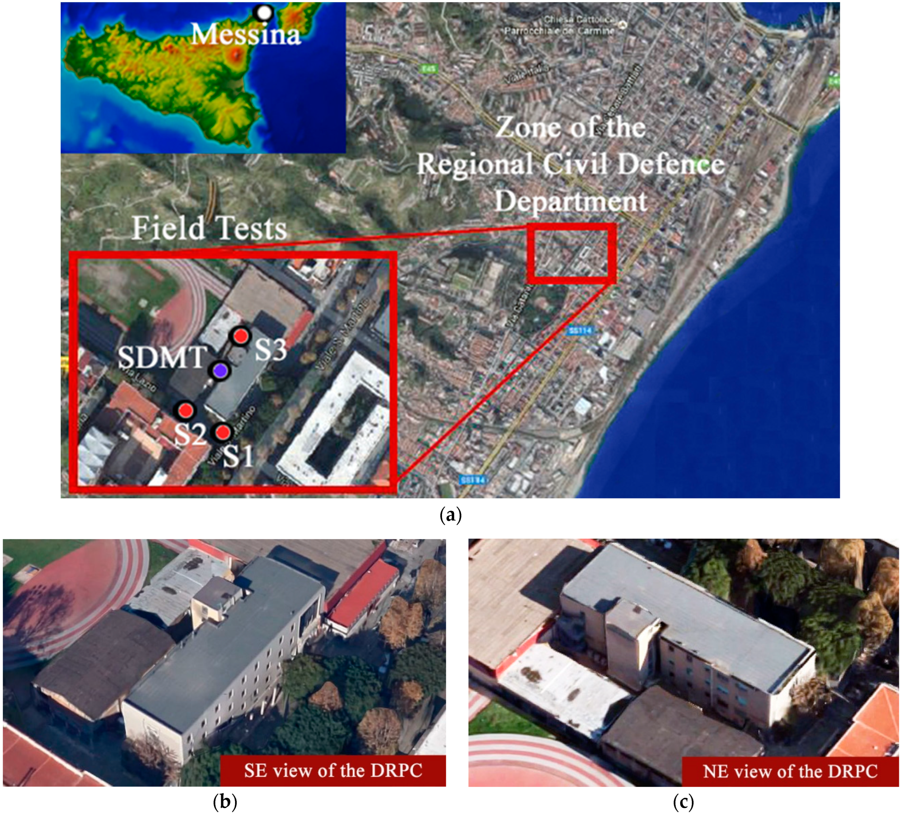
2. Seismicity of the Area

Eastern Sicily (Italy) has suffered numerous catastrophic earthquakes in the past (1169, 1693, 1783, 1818, 1908) [5]. Moreover, this area is prone to the additional risk of a damaging tsunami, as well as, liquefaction phenomena [17].

The Regional Department of Civil Defence (Dipartimento Regionale della Protezione Civile, DRPC) in the city of Messina (Sicily) is situated in a large coastal plain consisting of alluvial Holocene deposits [18] (Figure 1).

On 28th December 1908, an earthquake (Intensity MSC XI, Mw 7.24) occurred along the Strait of Messina between the eastern tip of Sicily and the western tip of Calabria. The Calabria and Messina earthquake was the most destructive seismic event of the 20th century in Italy with at least 80,000 fatalities [10]. The 1908 Messina and Reggio Calabria earthquake was used as the scenario earthquake.

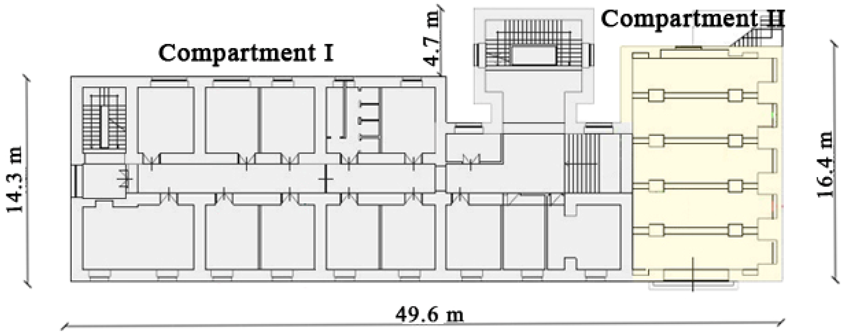
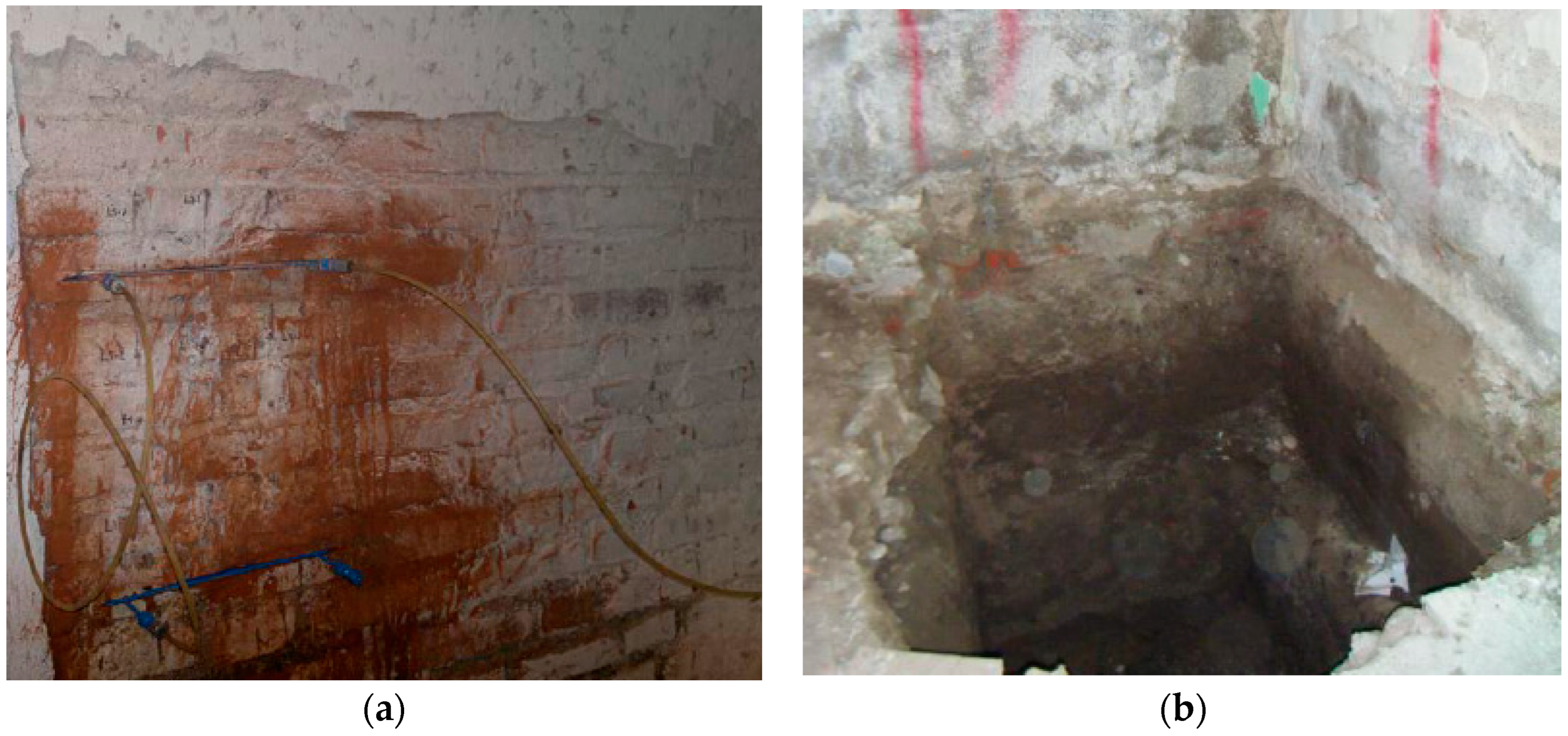
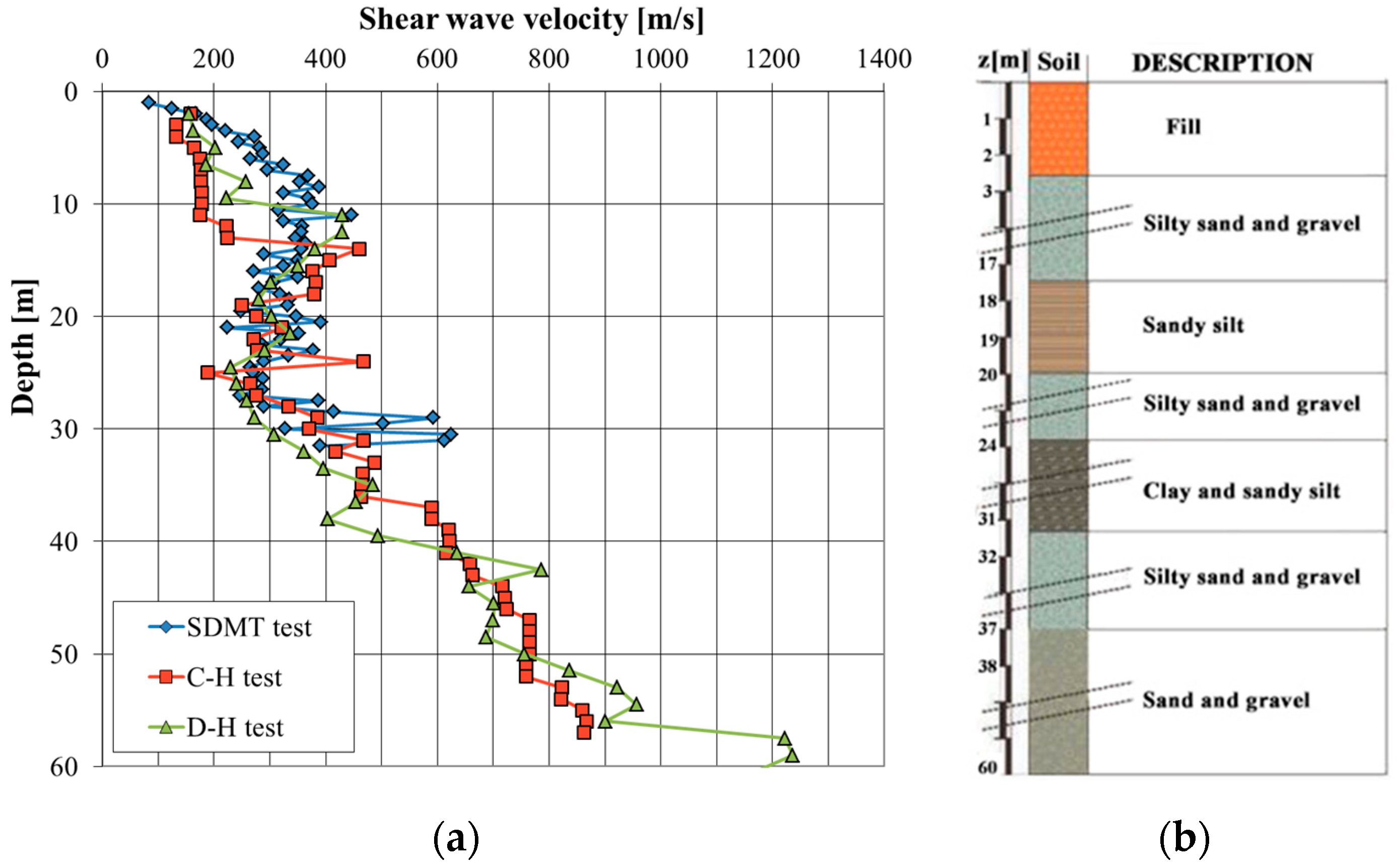
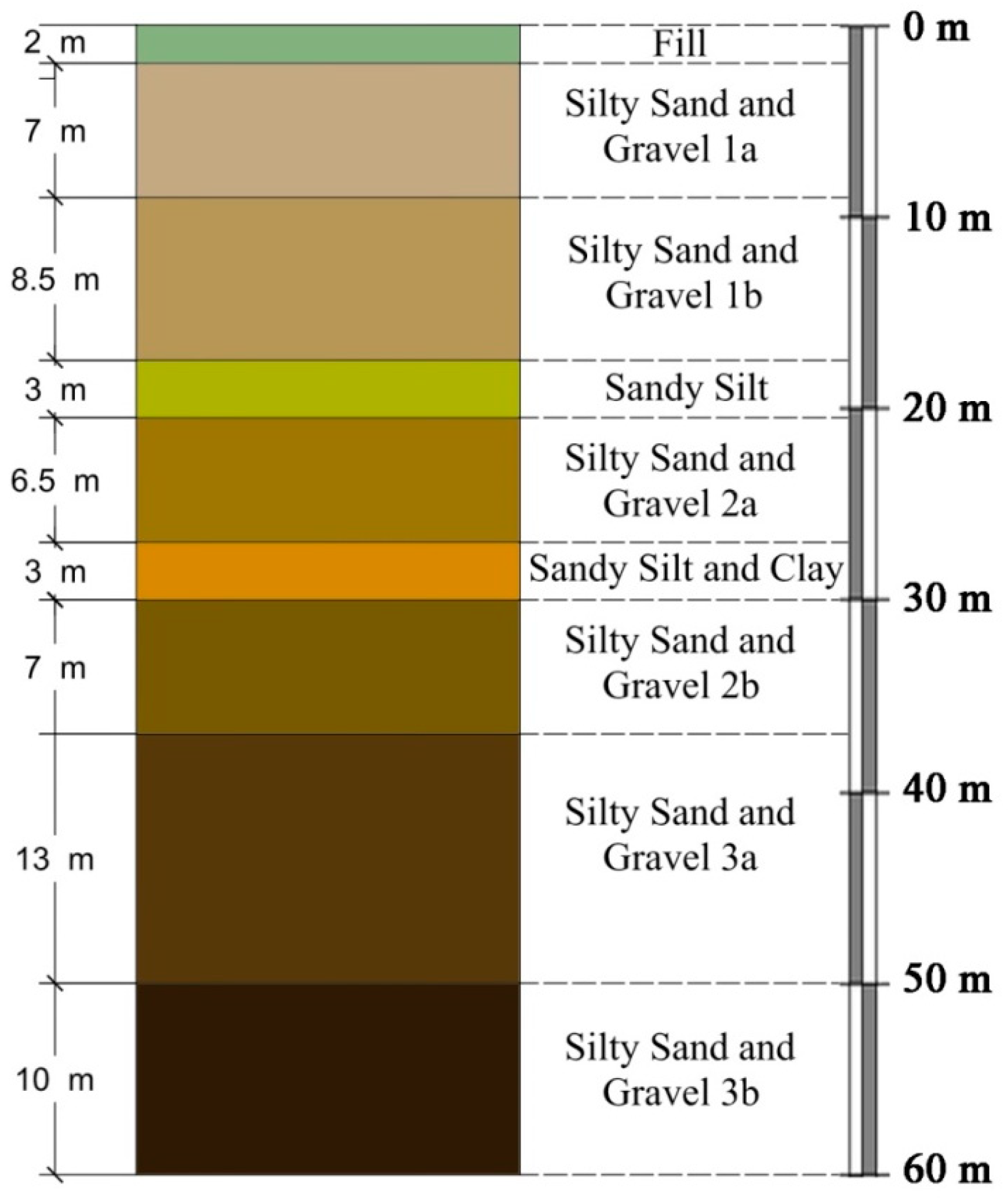
3. Description of the Building and Geotechnical Soil Properties

The DRPC building is rectangular in plan (Figure 2) and composed of four floors: an underground floor (at a depth of 1.60 m), a raised floor (at a height of 1.55 m), a first floor (at a height of 5.50 m) and a second floor (at a height of 9.50 m). In plan, two main compartments can be identified: one made up of perimeter and spine masonry walls (Compartment I) and the other made up of masonry columns with reinforced concrete beams and perimeter masonry walls (Compartment II). The foundation is composed of concrete beams for Compartment I and plinths for Compartment II, embedded to a depth of 2.9 m. A 3D view and axonometric cross section of the building are shown in Figure 3.

From the study of the construction typology, the structure has its origins in the first decades of the last century and was built after the calamitous seismic event of 1908 which destroyed a large part of the city of Messina. The building was designed, in all probability, according to the Regio Decreto Legge (RDL) no. 640 of 03/25/1935 that reduced the horizontal seismic force to 10% of the seismic weight, W, for buildings located in highly hazardous sites (Category I). Moreover, W was reduced to 40% for buildings in Category I. W was defined, according to the RDL no. 573 of 04/29/1915, as the sum of dead loads plus the quasi-permanent live loads, increased by 50%, to take into account the vertical seismic action [20].

The masonry walls were investigated by means of n. 7 double flat jack tests and n. 9 single flat jack tests (Figure 4a). The stiffness and mechanical properties of concrete foundations were obtained from n. 6 foundation inspection pits (Figure 4b), and compression tests were performed on n. 4 concrete samples (

Table 1. Stiffness and mechanical properties of the masonry and the concrete foundation.

	Parameter	Unit	Value
Masonry	Compressive strength	MPa	4.47
	Shear strength	MPa	0.39
	Elastic modulus	MPa	3120
	Volumetric weight	kN/m3	18
Concrete foundation	Cylindrical resistance	MPa	7.30
	Elastic modulus	MPa	20,017

).

For the geotechnical characterization of the subsoil, in situ and laboratory tests were carried out in the DRPC area. Three boreholes, labeled S1, S2 and S3 (Figure 1a), showed that the DRPC area mainly consists of silty sand and gravel with horizons of clay and sandy silt (Figure 5b). In order to obtain the shear wave velocity, V_S, with depth, n. 1 down-hole test, n. 1 cross-hole test and n. 1 Seismic Dilatometer Marchetti Test (SDMT) (Figure 1a) were performed. V_S values, derived from geophysical tests, are plotted against depth in Figure 5a.

Moreover, the following laboratory tests were performed: n. 6 Direct Shear Tests (DST), n. 2 Consolidated Undrained Triaxial Tests (CUTxT), n. 4 Resonant Column Tests (RCT) and n. 4 Cyclic Loading Torsional Shear Tests (CLTST). Based on the laboratory tests, the main index properties encountered in the area are reported in

Table 2. Index properties for the investigated area.

Sample	z [m]	γ [kN/m3]	wn [%]	Gs	e	n	Sr [%]
S1C1	7.00–7.40	18.34	11.93	2.79	0.67	0.40	49.95
S2C1	3.00–3.50	18.63	18.90	2.75	0.72	0.42	72.03
S2C2	6.00–6.40	19.81	13.19	2.74	0.54	0.35	67.15
S3C1	5.50–6.00	19.12	15.08	2.79	0.65	0.39	64.87
S3C2	14.60–15.00	19.91	12.51	2.74	0.52	0.34	65.57
S3C3	21.00–21.40	16.18	33.61	-	-	-	-
S3C4	27.00–27.50	17.95	39.78	2.76	1.11	0.53	99.11

z = depth, γ = unit weight; w_n = natural water content, G_s = specific gravity, e = void index, n = porosity, S_r = degree of saturation.

.

Figure 6 presents the deviator stress–axial strain curves obtained from CUTxT performed on sample S3C4 (sample C4 retrieved from 27.00–27.50 m in borehole S3) under different values of p′_c (200 kPa, 400 kPa and 600 kPa) for a back pressure of 190 kPa.

Values of the normalized shear modulus G/G₀ and damping ratio ξ [%] versus γ [%] for samples S1C1 (sample C1 retrieved from 7.00–7.50 m in borehole S1) and S3C4 (sample C4 retrieved from 27.00–27.50 m in borehole S3) obtained by RTC and CLTST, respectively, are reported in Figure 7.

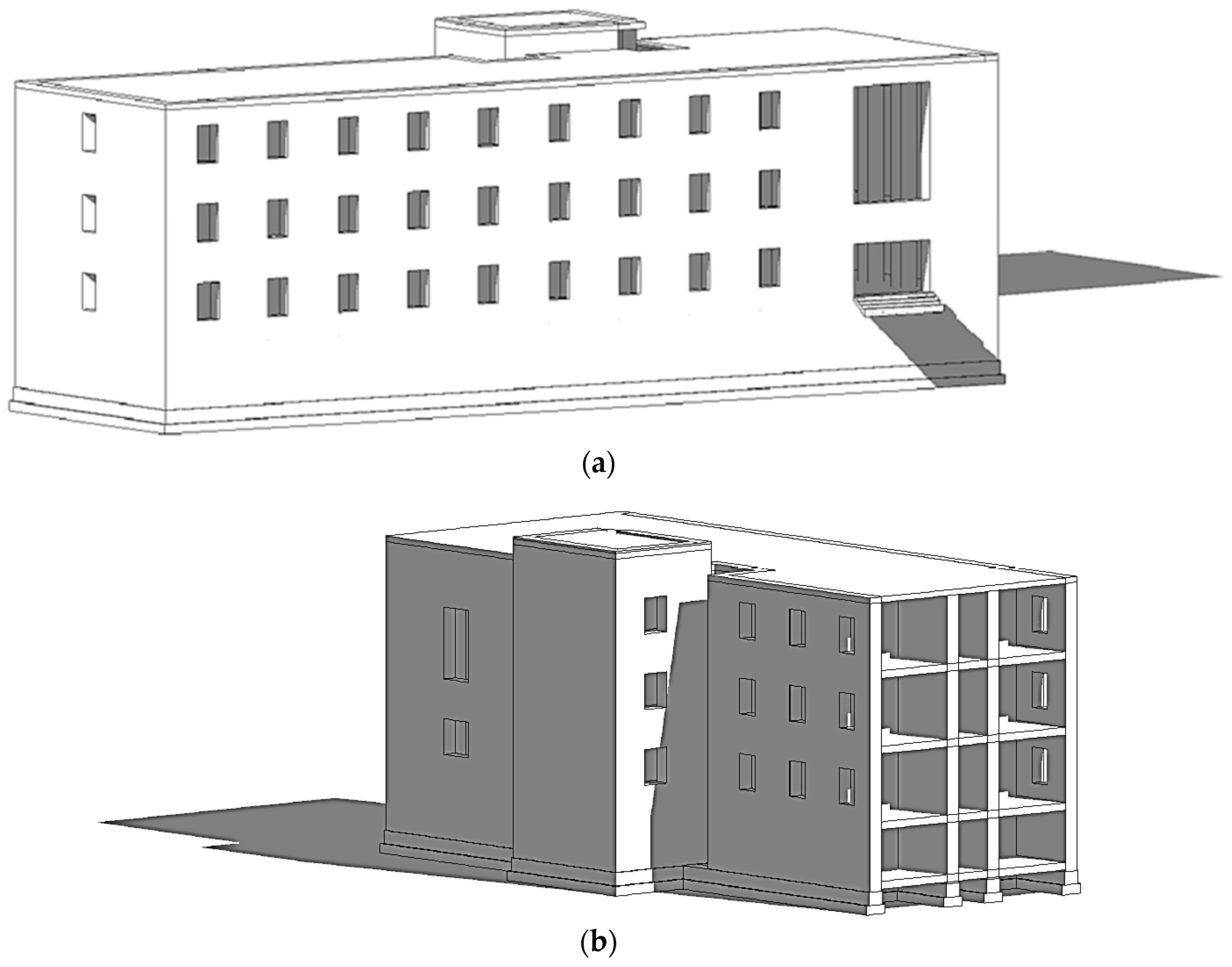
4. Coupled Soil–Structure Model

Fully coupled FEM analyses were carried out using PLAXIS3D. From in situ investigations, nine layers were identified (Figure 8) to define the 3D soil model (446 m × 171 m × 60 m). The depth of the conventional bedrock (V_S > 800 m/s according to the Italian seismic code [4]) was fixed to 60 m below the ground surface.

Seismograms were applied along the x-direction. In order to reduce boundary effects, the length of the soil model was chosen to equal 9 times the footprint of the building. The soil elements in 3D finite element mesh are modeled as 10-node tetrahedral elements. The maximum dimension of the mesh elements, h_max, respects the following condition [21]:

$$h_{max}\le \frac{V_{s,min}}{6÷8f_{max}}$$

(1)

where f_max is the maximum significant frequency of dynamic input (equal to 25 Hz) and V_S,min is the lowest wave velocity (equal to 146 m/s).

Relevant previous studies [7,22] showed the important role of boundary conditions in numerical modeling. In this regard, default fixities were applied to generate the initial stresses due to gravity loading, and free-field and compliant base boundary conditions [23,24] were considered for the dynamic phase (Figure 9).

The free-field boundary reproduces the propagation of waves into the far field with minimum reflections. The domain is reduced to the area of interest (main domain) and the free-field motion is imposed to the boundaries by means of free-field elements. The motion is transferred from the free-field elements to the main domain by employing equivalent normal and shear forces. The compliant base boundary [25] reproduces the continuation of waves into the deep soil with minimum reflections. Two dashpots are added in the normal and shear direction at each node of the model boundary to adsorb downward propagating waves [23,24].

Moreover, previous research [26,27] indicates that the mesh size of the FEM may greatly affect the numerical results. For this reason, in order to validate the 3D FEM, including the dynamic boundary conditions, the approach reported by Gaudio [28] was employed. Numerical analyses were carried out in three steps. In the first step, local site response analyses were performed using the 1D equivalent codes EERA [29] and STRATA [30], taking into account a soil column. In the second step, values of the shear modulus, G, and the damping ratio, D, evaluated by 1D linear equivalent codes, were inserted in the PLAXIS3D software. Finally, results obtained by the 1D equivalent linear method were compared with those derived by means of PLAXIS 3D finite element software (Version 21.01.00.479), assuming a linear visco-elastic soil behavior, to optimize the mesh size and check the boundary conditions.

Structural objects were simulated as volumes in PLAXIS3D by a visco-elastic constitutive model. Material properties derived from building tests were used for masonry and concrete. Conventional properties were considered for the hollow bricks and concrete floors and for the reinforced concrete elements (

Table 3. Properties of the structural objects.

	Parameter	Value	Unit
Masonry	Unit weight	18	kN/m3
	Young’s modulus	3,120,000	kN/m2
	Poisson’s ratio	0.20	-
	Damping	8	%
Concrete	Unit weight	24	kN/m3
	Young’s modulus	20,017,000	kN/m2
	Poisson’s ratio	0.25	-
	Damping	5	%
Hollow bricks and concrete floors	Unit weight	18	kN/m3
	Young’s modulus	20,000,000	kN/m2
	Poisson’s ratio	0.20	-
	Damping	5	%
Reinforced concrete elements	Unit weight	25	kN/m3
	Young’s modulus	28,500,000	kN/m2
	Poisson’s ratio	0.25	-
	Damping	5	%

).

For a proper simulation of the SSI, interface elements were added to the foundation. An elastic–plastic model was used to describe their behavior by adopting an appropriate value for the strength reduction factor, R_inter, equal to 2/3. The finite element mesh of the coupled soil–structure system is shown in Figure 10.

5. Selected Seismic Input

Numerical analyses were performed using a deterministic approach. Although the application of a probabilistic approach can provide valuable help in selecting sets of accelerograms [5], a deterministic approach is preferred in areas with moderate to high seismic risk [10].

A parametric study considering three different seismograms related to the 1908 seismic event was performed. The selected seismic inputs used for the numerical analyses are bedrock outcrop motions. In this regard, it is important to highlight that the ‘within motion’ is the superposition of the upward and downward propagating waves at the boundary between two layers, while the ‘outcrop motion’ is twice the upward propagating waves at the free field surface [31]. Therefore, in PLAXIS3D, the seismic input applied at the compliant base has to be ½ of the bedrock outcrop motion in order to consider only the upward-propagating waves. The site effects were evaluated by comparing the bedrock outcrop motions with the motion obtained at the surface from numerical analyses, as reported in Section 7.

A single planar fault was employed to derive the first source model [32]. Normal faulting with an ESE–WNW extension, as the dominant mode of deformation of the Calabrian arc, was considered to obtain the second source model [33]. The third source model, included in the Italian Database of Individual Seismogenic Sources (DISS) by Basili et al. [34], is a low-angle normal fault obtained by Valensise and Pantosti [35]. The three synthetic seismograms (Figure 11) have a peak ground acceleration (PGA) of 0.456 g, 0.337 g and 0.293 g, respectively, corresponding to different return periods in the Italian technical standard of construction NTC [4]: 1950 years, 950 years and 712 years.

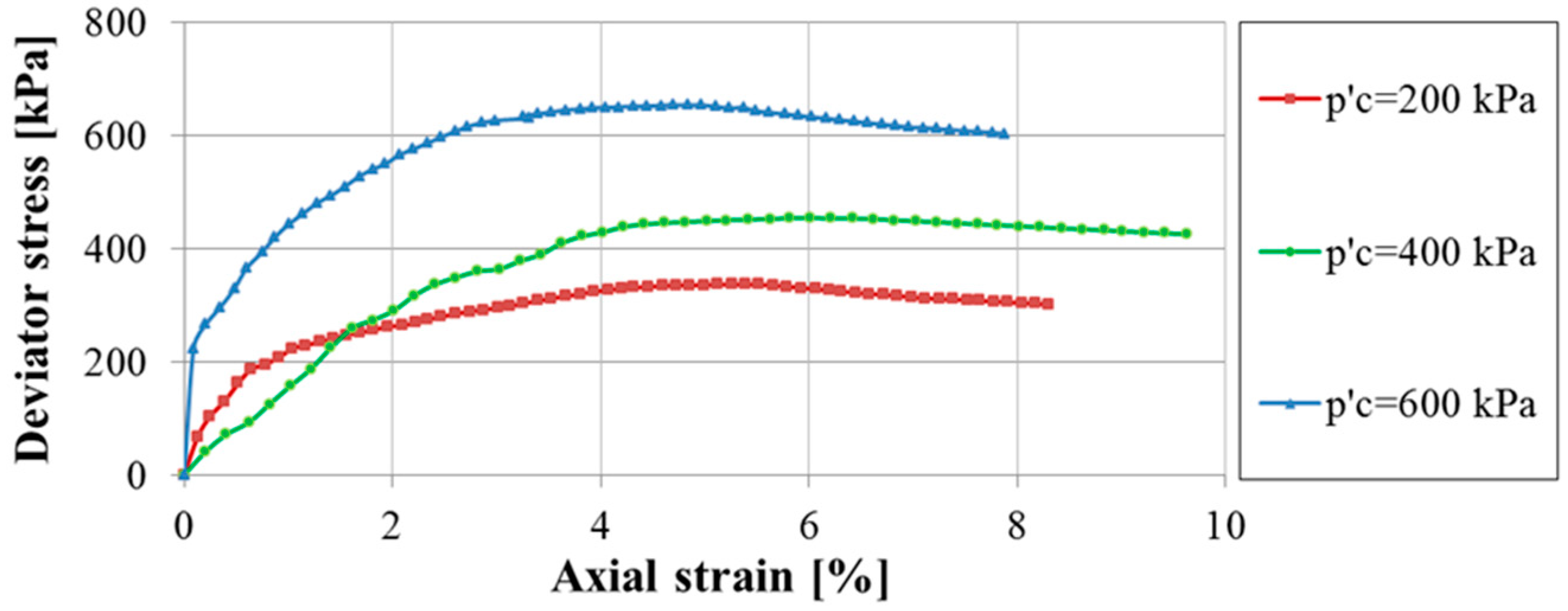
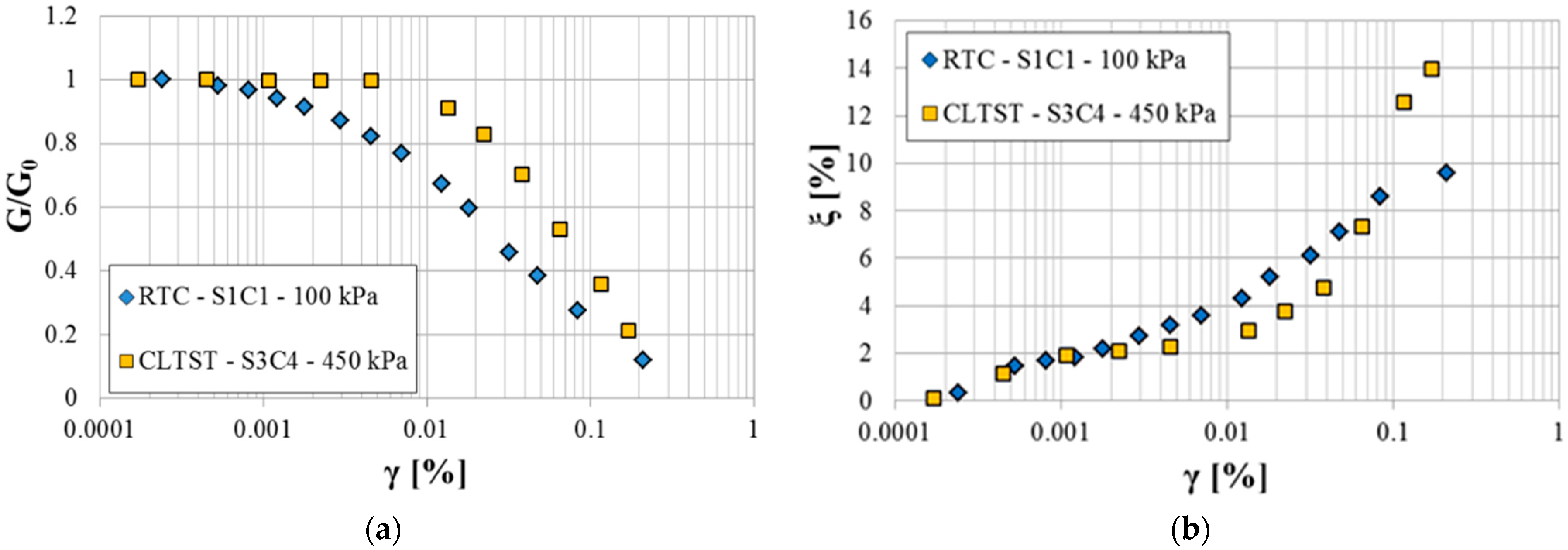
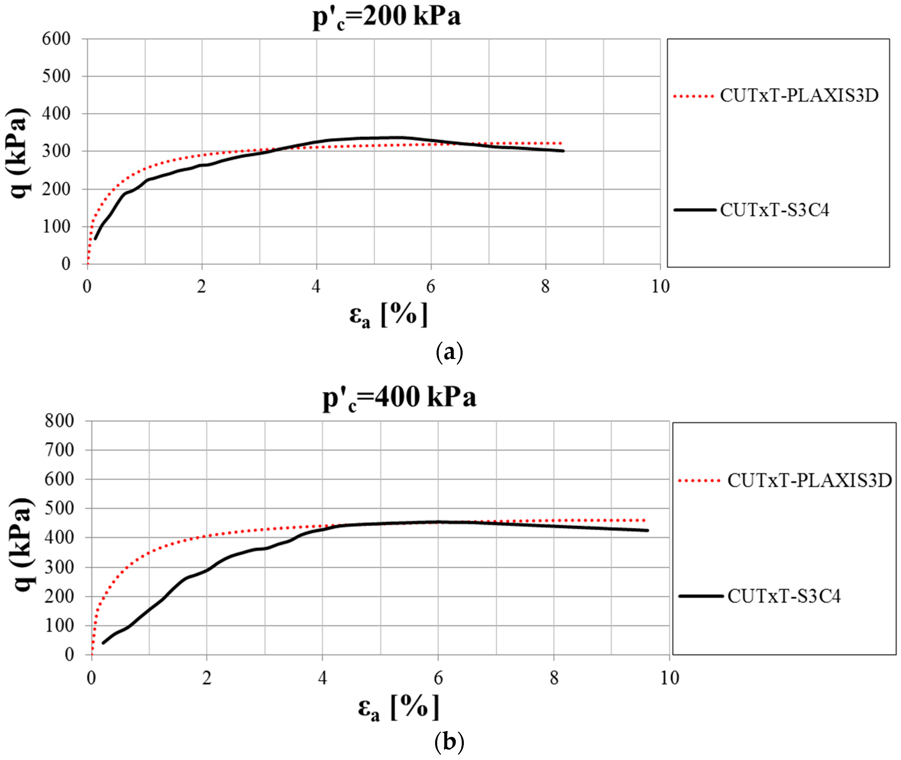
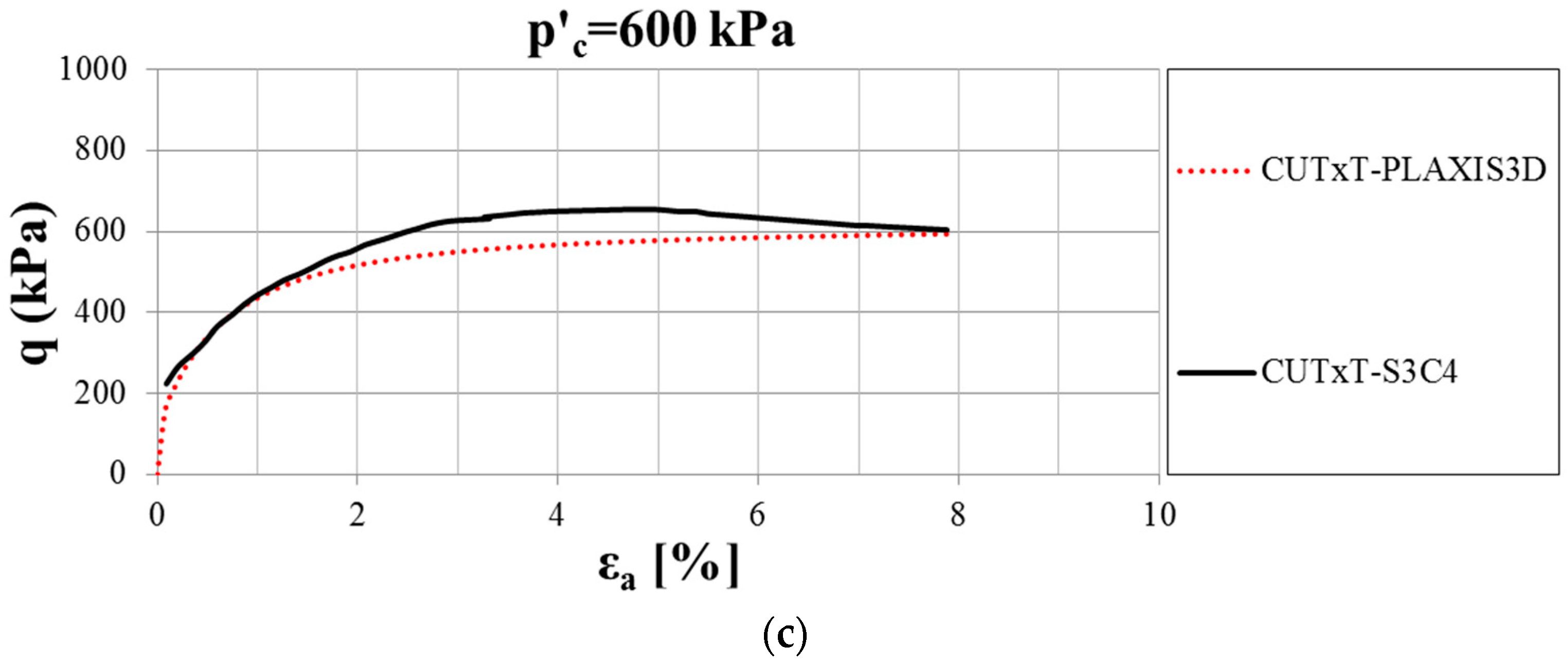
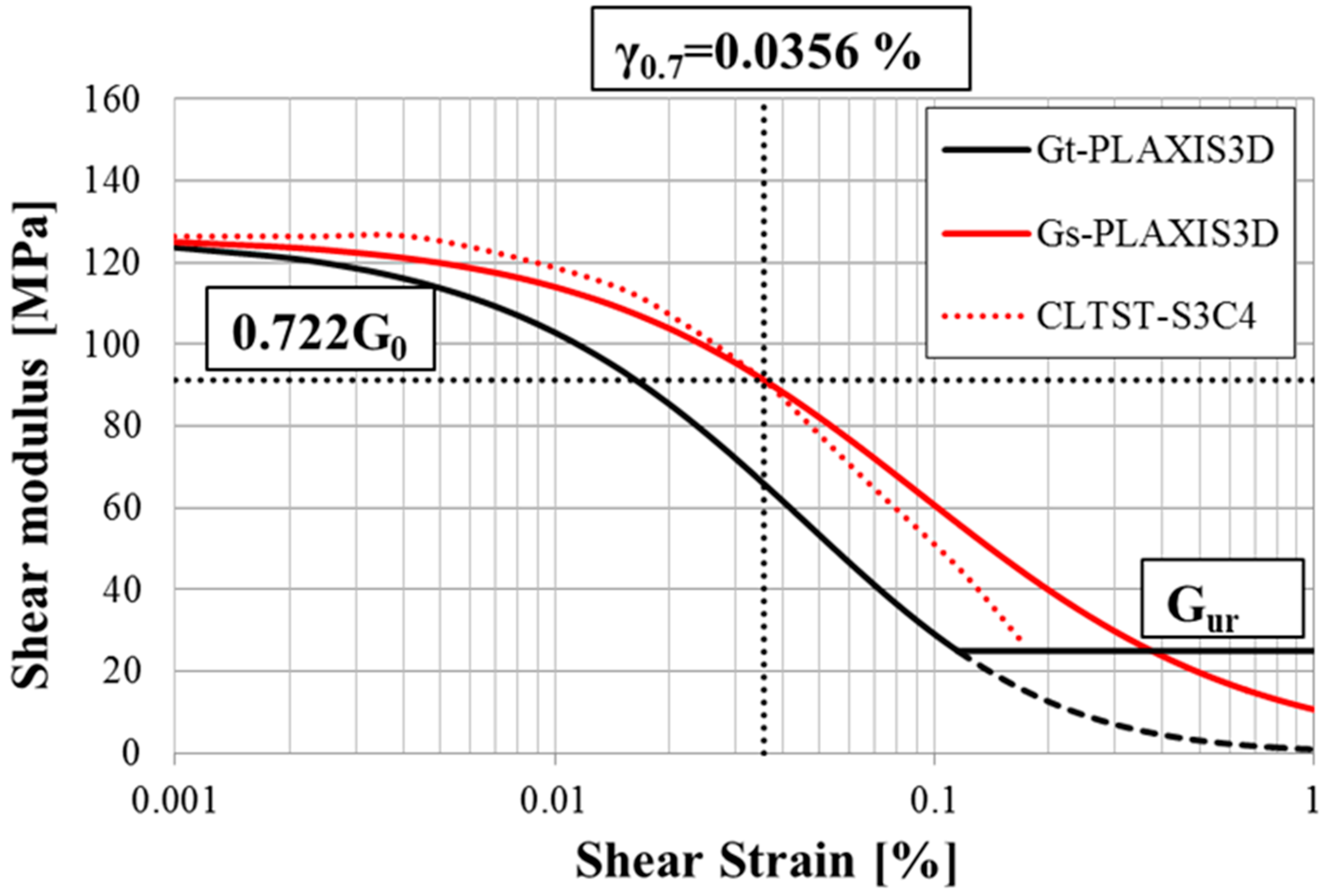
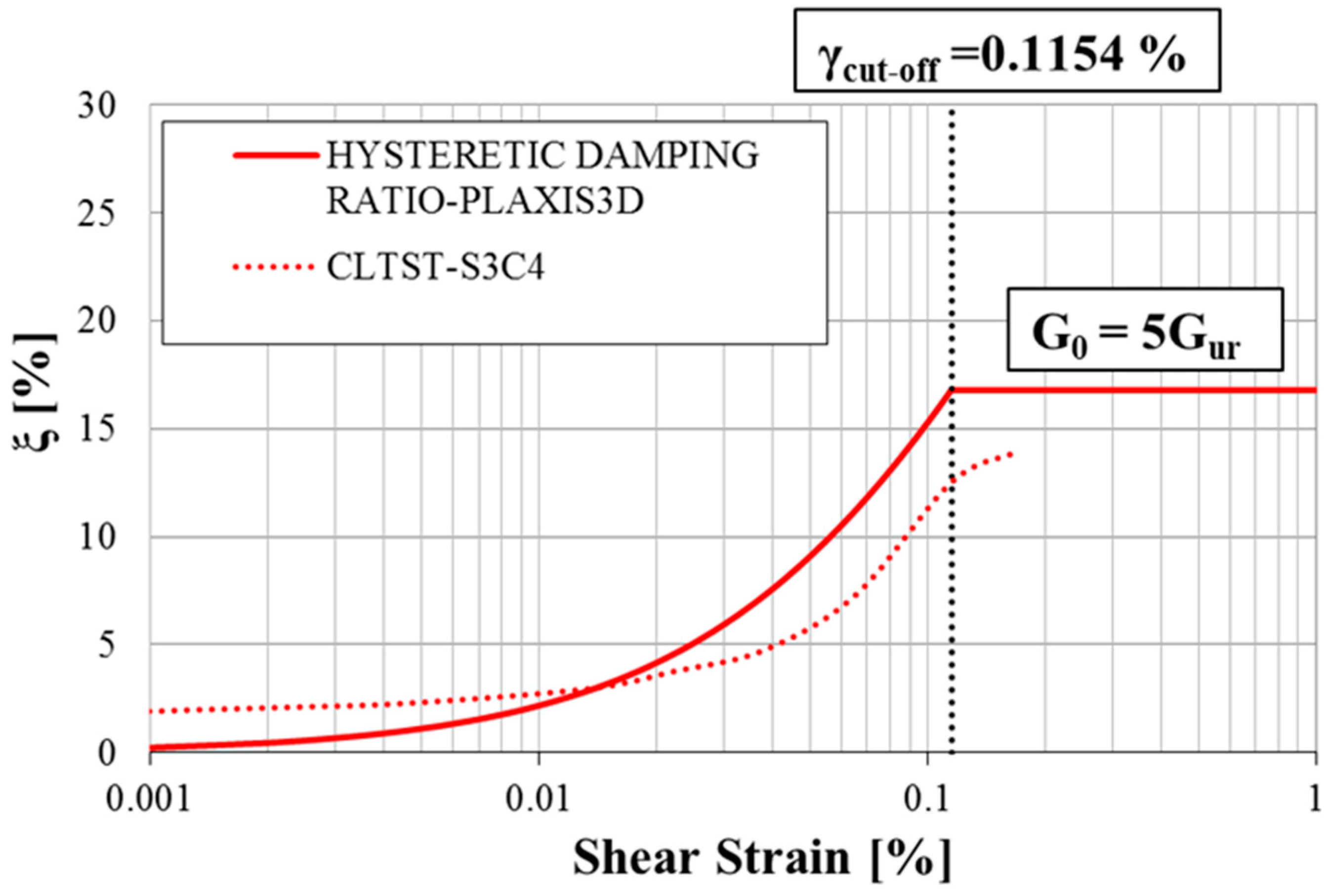
6. Calibration of the HS Small Model

In this study, the input parameters of the HS small model were calibrated to the geophysical tests (Figure 5a), the consolidated undrained triaxial tests (Figure 6) and the dynamic tests (Figure 7) as presented in

Table 4. In situ and laboratory tests used for the calibration of the model.

Layers	CUTxT	VS Values from Geophysical Tests [m/s]	Dynamic Tests
Fill	CUTxT-S3C1	146	RTC-S1C1
Silty sand and gravel 1a	CUTxT-S3C1	176	RTC-S1C1
Silty sand and gravel 1b	CUTxT-S3C1	335	RTC-S1C1
Sandy silt	CUTxT-S3C1	318	RTC-S1C1
Silty sand and gravel 2a	CUTxT-S3C1	288	RTC-S1C1
Sandy silt and clay	CUTxT-S3C4	260	CLTST-S3C4
Silty sand and gravel 2b	CUTxT-S3C4	457	CLTST-S3C4
Silty sand and gravel 3a	CUTxT-S3C4	665	CLTST-S3C4
Silty sand and gravel 3b	CUTxT-S3C4	911	CLTST-S3C4

.

The HS small model requires three stiffness moduli at the reference pressure, p^ref, namely E₅₀^ref, E_ur^ref and E_oed^ref, that are stress-level dependent, according to the following expressions:

$$E_{oed}={E_{oed}}^{ref}{\left(\frac{{{\sigma }^{\prime }}_1}{p^{ref}}\right)}^m$$

(2)

$$E_{50}={E_{50}}^{ref}{\left(\frac{{{\sigma }^{\prime }}_3}{p^{ref}}\right)}^m$$

(3)

$$E_{ur}={E_{ur}}^{ref}{\left(\frac{{{\sigma }^{\prime }}_3}{p^{ref}}\right)}^m$$

(4)

where ${{\sigma }^{\prime }}_1$ and ${{\sigma }^{\prime }}_3$ are the major and minor principal effective stresses, and m is the power for stress-level dependency of stiffness.

Moreover, the following ratios were adopted:

$${E_{50}}^{ref}{{=E}_{oed}}^{ref}$$

(5)

$${E_{ur}}^{ref}={{3E}_{oed}}^{ref}$$

(6)

For the all-soil layers, the exponent, m, and Poisson’s ratio for unloading–reloading, ν_ur, were assumed to be equal to 0.5 and 0.2, respectively.

In order to determine the stiffness and strength parameters of the HS small model, CUTxT were simulated using PLAXIS3D software. In Figure 12, the comparison between the calibrated model for the sandy silt and clay layer, as an example, and the results derived by CUTxT for sample S3C4 under different values of p′_c (200 kPa, 400 kPa, 600 kPa) for a back pressure of 190 kPa is reported.

To describe the variation of stiffness with strain, two additional parameters have been considered: the reference shear modulus at very low strain, G₀^ref, and the shear strain level, γ_0.7, at which the secant shear modulus, G_S, is reduced to 72.2% of G₀. The stress dependency of the shear modulus G₀ is given by the following expression:

$$G_0={G_0}^{ref}{\left(\frac{{{\sigma }^{\prime }}_3}{p^{ref}}\right)}^m$$

(7)

where values of G₀ are obtained from the shear wave velocity (Table 4) and the soil density (Table 2) according to the following equation:

$$G_0=\rho V_S^2$$

(8)

The values of γ_0.7 were derived from dynamic tests (Table 4). In the HS small model, the secant shear modulus, G_s, and the tangent shear modulus, G_t, are given by Equations (9) and (10), respectively:

$$\tau =G_s\gamma =\frac{G_0\gamma }{1+0.385\frac{\gamma }{{\gamma }_{0.7}}}$$

(9)

$$G_t=\frac{G_0}{{\left(1+0.385\frac{\gamma }{{\gamma }_{0.7}}\right)}^2}$$

(10)

G_t is limited by the value of the unloading–reloading stiffness, G_ur, which is linked to E_ur and ν_ur by the following equation:

$$G_{ur}=\frac{E_{ur}}{2\left(1+{\nu }_{ur}\right)}$$

(11)

Figure 13 shows a comparison between the calibrated model for the sandy silt and clay layer, as an example, and the decay curve of the shear modulus as a function of the level of deformation obtained from the CLTST performed on sample S3C4.

In the HS small model, the hysteretic damping ratio, ξ, is defined as [36]:

$$\xi =\frac{E_D}{4\pi E_S}$$

(12)

where E_D and E_S are the dissipated energy and the stored energy, respectively, formulated as:

$$E_D=\frac{4G_0{\gamma }_{0.7}}{0.385}\left(2{\gamma }_c-\frac{{\gamma }_c}{1+\frac{{\gamma }_{0.7}}{0.385{\gamma }_c}}-\frac{2{\gamma }_{0.7}}{0.385}ln\left(1+\frac{0.385{\gamma }_c}{{\gamma }_{0.7}}\right)\right)$$

(13)

$$E_s=\frac{1}{2}{G}_S{\gamma }_c^2=\frac{G_0{{\gamma }_c}^2}{2+2\frac{{\gamma }_c}{{\gamma }_{0.7}}0.385}$$

(14)

The cut-off shear strain, γ_cut-off, is given by the following expression:

$${\gamma }_{cut\text{-}off}=\frac{1}{0.385}\left(\sqrt{\frac{G_0}{G_{ur}}}-1\right){\gamma }_{0.7}$$

(15)

In Figure 14, the hysteretic damping in the HS small model is compared with the increase in damping as a function of the level of deformation obtained from the CLTST performed on sample S3C4.

Table 5. Input parameters of the HS small model.

Parameter	Symbol	Sandy Silt and Clay Layer	Unit
General
Material model	-	HS small	-
Saturated unit weight of soil	γsat	18	kN/m3
Stiffness parameters
Secant stiffness in standard drained triaxial test	E50ref	20,000	kN/m2
Tangent stiffness for primary oedometer loading	Eoedref	20,000	kN/m2
Unloading/reloading stiffness	Eurref	60,000	kN/m2
Reference stress for stiffness	pref	200	kN/m2
Power for stress-level dependency of stiffness	m	0.5	-
Additional stiffness parameters
Reference shear modulus at very small strains	G0ref	126,388	kN/m2
Threshold shear strain at which GS = 0.722 G0	γ0.7	0.000356	-
Strength parameters
Cohesion	c′	38	kN/m2
Friction Angle	φ′	23	°

reports the input parameters of the calibrated model, i.e., for the sandy silt and clay layer. Values of the parameters of the HS small model that describe the nonlinear behavior of the soil are presented in

Table 6. Parameters of the HS small model for soil non linearity.

Layer	G0ref [kN/m2]	pref [kN/m2]	γ0.7
Fill	46,699	100	0.000121
Silty sand and gravel 1a	60,638	100	0.000121
Silty sand and gravel 1b	242,569	100	0.000121
Sandy silt	205,403	100	0.000121
Silty sand and gravel 2a	160,979	100	0.000121
Sandy silt and clay	126,388	200	0.000356
Silty sand and gravel 2b	367,659	200	0.000356
Silty sand and gravel 3a	706,657	200	0.000356
Silty sand and gravel 3b	1,209,396	200	0.000356

for all layers.

7. Analysis of the Results

The free-field (FF) condition was compared with the SSI condition (Figure 9) to analyze how the SSI modifies the dynamic response. These findings are of great importance in the field of seismic geotechnical engineering, showing the important role of the SSI effects and nonlinearity in the retrofitting and/or improving of existing structures.

Figure 15 shows the results obtained in terms of maximum accelerations with depth using as input the three 1908 seismograms. Results of numerical analyses highlight that the presence of the structure induces higher values of the maximum acceleration compared with the FF condition at the foundation level.

Figure 16 reports the results at the surface in terms of spectral accelerations obtained by setting a structural damping of 5%. Considering the Amoruso seismogram, for the period of the structure (T_STRU = 0.39 s from modal analysis), a spectral acceleration of 1.07 g was obtained for the SSI alignment, while a lower value of 0.78 g was found for the FF condition (Figure 16a). Thus, in this case, the SSI leads to a designed acceleration greater than that required in the FF condition.

The Tortorici seismogram has a PGA of 0.337 g, corresponding to the limit state for the safeguard of life (SLV) and Class IV (public buildings of strategic importance) according to the approach proposed by NTC [4]. Therefore, for comparison, the elastic response spectrum provided by the NTC [4] is also shown.

Based on the response spectra obtained using the Tortorici seismogram (Figure 16b), spectral accelerations of 0.68 g (FF condition) and 0.72 g (SSI condition) were found for T_STRU = 0.39 s, while according to the NTC [4], a greater value of 0.99 g was achieved. Results show that the NTC [4] spectrum is more conservative for the period under consideration. Moreover, in both cases (Amoruso and Tortorici seismograms) the spectral accelerations are higher considering the full-coupled analyses.

The results obtained adopting the DISS Messina Straits seismogram (Figure 16c) show a spectral acceleration Se(T_STRU)_FF = 0.55 g for the FF condition and Se(T_STRU)_SSI = 0.47 g for the SSI condition. Therefore, in this case, the SSI has a beneficial effect. Figure 17 summarizes the values of spectral acceleration for the period of the structure using as input the three 1908 seismograms.

Figure 18 shows the amplification functions, A(f), evaluated as the ratio between the Fourier spectrum at the surface level and the Fourier spectrum of the input motions applied at the base of the model. The main resulting frequencies for SSI and FF conditions are compared with the first and the second predominant frequencies of the input motions, and with the frequency of the structure. Considering the Amoruso seismogram (Figure 18a), it is possible to observe that the first predominant frequency of the input motion (f_p(I) = 3.37 Hz) is near to the following resulting frequencies for FF and SSI conditions: f_FF(III) = f_SSI(II) = 3.50 Hz. Moreover, the SSI has a positive effect because the second resulting frequency for the FF condition (f_FF(II) = 2.55 Hz) is very close to the frequency of the structure (f_STRU = 2.5 6Hz). Figure 18b shows that for the Tortorici seismogram, the first resulting frequencies f_FF(I) = f_SSI(I) = 1.17 Hz are close to the second predominant frequency of the input motion f_p(II) = 0.97 Hz. Furthermore, the second main A(f) peak moves towards lower frequencies considering the full-coupled analysis: f_FF(II) = 3.55 Hz and f_SSI(II) = 2.97 Hz and, consequently, further from the first predominant frequency of the input motion (f_p(I) = 3.37 Hz). In both cases, resulting frequencies are far from the frequency of the structure. The results obtained using the DISS Messina Straits seismogram (Figure 18c) show that the first resulting frequency for the SSI condition f_SSI(I) = 1.44 Hz is closer to the second fundamental input frequency (f_p(II) = 1.58 Hz), and the second main A(f) peaks f_FF(II) = f_SSI(II) = 2.97 Hz are near to the frequency of the structure.

As mentioned above, the period of the structure, T_STRU, was determined from modal analysis. In particular, the value of 0.39 s was found. However, the presence of soil leads to period elongation and, in turn, affects the shift of the resonance. Therefore, using the approach reported by Massimino et al. [37], the period elongation due to the presence of the soil, T_STRU,SSI, was also evaluated by the amplification function derived from the ratio between the Fourier amplitude spectra at the top and at the bottom of the structure resting on the soil. The value of T_STRU,SSI = 0.44 s (f_STRU,SSI = 0.27 Hz) was obtained. In this case, the period elongation has positive effects, since the frequency of the structure, f_STRU,SSI, tends to shift from the resulting frequencies for the SSI condition and from the predominant frequencies of the input motion. Similar considerations were also formulated by Massimino et al. [8].

The deformed mesh at the end of the dynamic phase, displayed in Figure 19 for the Amoruso seismogram, as an example, shows the same behavior for each seismogram.

The time histories of the settlement at the foundation level and the free field soil surface are presented in Figure 20. Moreover, vertical displacements for the central alignment under the structure (SSI) are also reported for the depth of 6.6 m (silty sand and gravel 1a layer) and 9.0 m (silty sand and gravel 1b).

It can be observed that instantaneous settlements of about 0.025 m occur at the beginning of the dynamic time at the foundation level considering the SSI condition, while they are zero at the ground surface in the FF condition. Values tend to increase in correspondence with the acceleration peaks of each seismogram. At the end of the dynamic time, settlements of 0.052 m, 0.049 m and 0.043 m occur for the Amoruso (Figure 20a), Tortorici (Figure 20b) and DISS Messina Straits (Figure 20c) seismograms, considering the SSI condition. On the other hand, they are reduced to 0.025 m, 0.037 m and 0.015 m for the Amoruso (Figure 20a), Tortorici (Figure 20b) and DISS Messina Straits (Figure 20c) seismograms at the FF soil surface.

Moreover, it is possible to observe that the vertical displacements decrease with depth along the SSI alignment reaching the value of about 0.015 m at a depth of 9.0 m.

Figure 21a, Figure 22a and Figure 23a present the stress–strain hysteretic loops for each seismogram at a depth of 0.3 m in order to represent the soil behavior near the surface without the presence of the structure. Figure 21b,c, Figure 22b,c and Figure 23b,c report the shear stress vs. shear strain curves for the SSI alignment at a depth of 3.1 m in order to consider the soil behavior at the foundation level and at a depth of 10 m to study the variation along the SSI alignment. A comparison of the behavior at the different depths shows that shear stresses increase at a depth of 10 m, reaching values of 50.2 kPa, 38.2 kPa and 44.2 kPa for the Amoruso (Figure 21c), Tortorici (Figure 22c) and DISS Messina Straits (Figure 23c) seismograms, respectively. The maximum shear strain occurs at the foundation level, achieving values of 0.26%, 0.29% and 0.49% for the Amoruso (Figure 21a), Tortorici (Figure 22a) and DISS Messina Straits (Figure 23a) seismograms, respectively.

Moreover, a comparison between the FF field condition (Figure 21a, Figure 22a and Figure 23a) and the SSI condition at the foundational level (Figure 21b, Figure 22b and Figure 23b) shows that the presence of the structure provides a highly nonlinear response demonstrating the crucial importance of taking into account the soil nonlinearity in seismic SSI problems.

8. Discussion

The main findings derived from the comparison between the central alignment under the structure and the FF condition are summarized as follows.

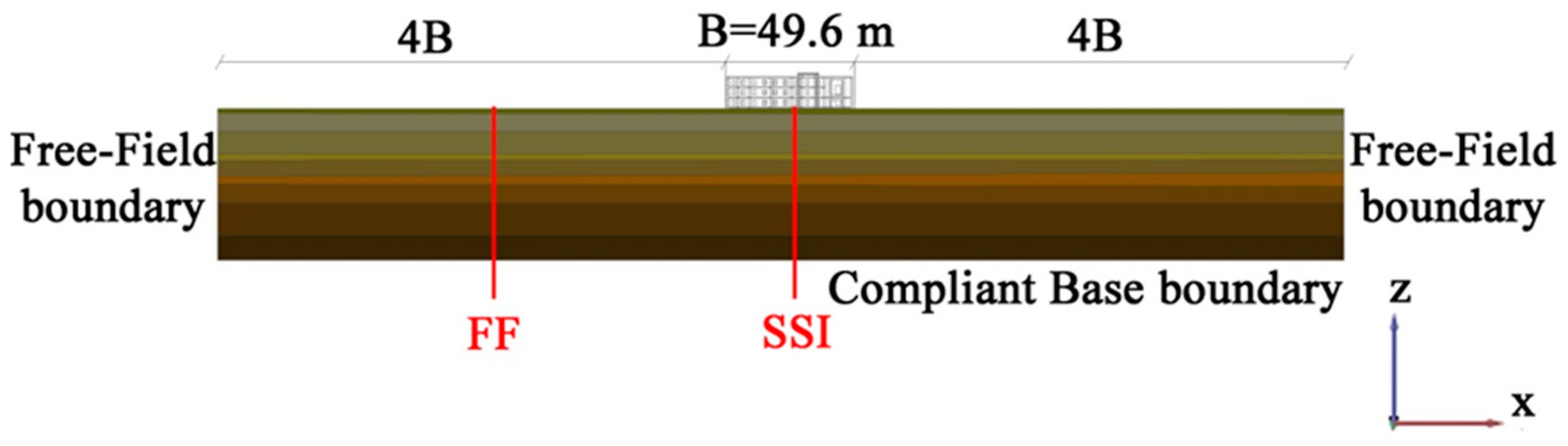
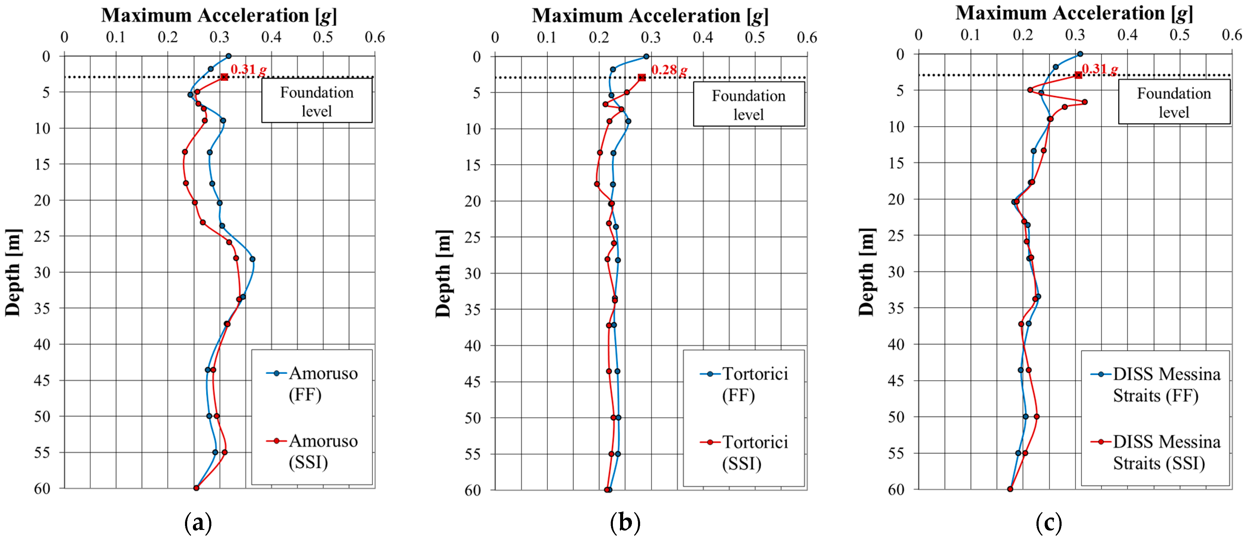
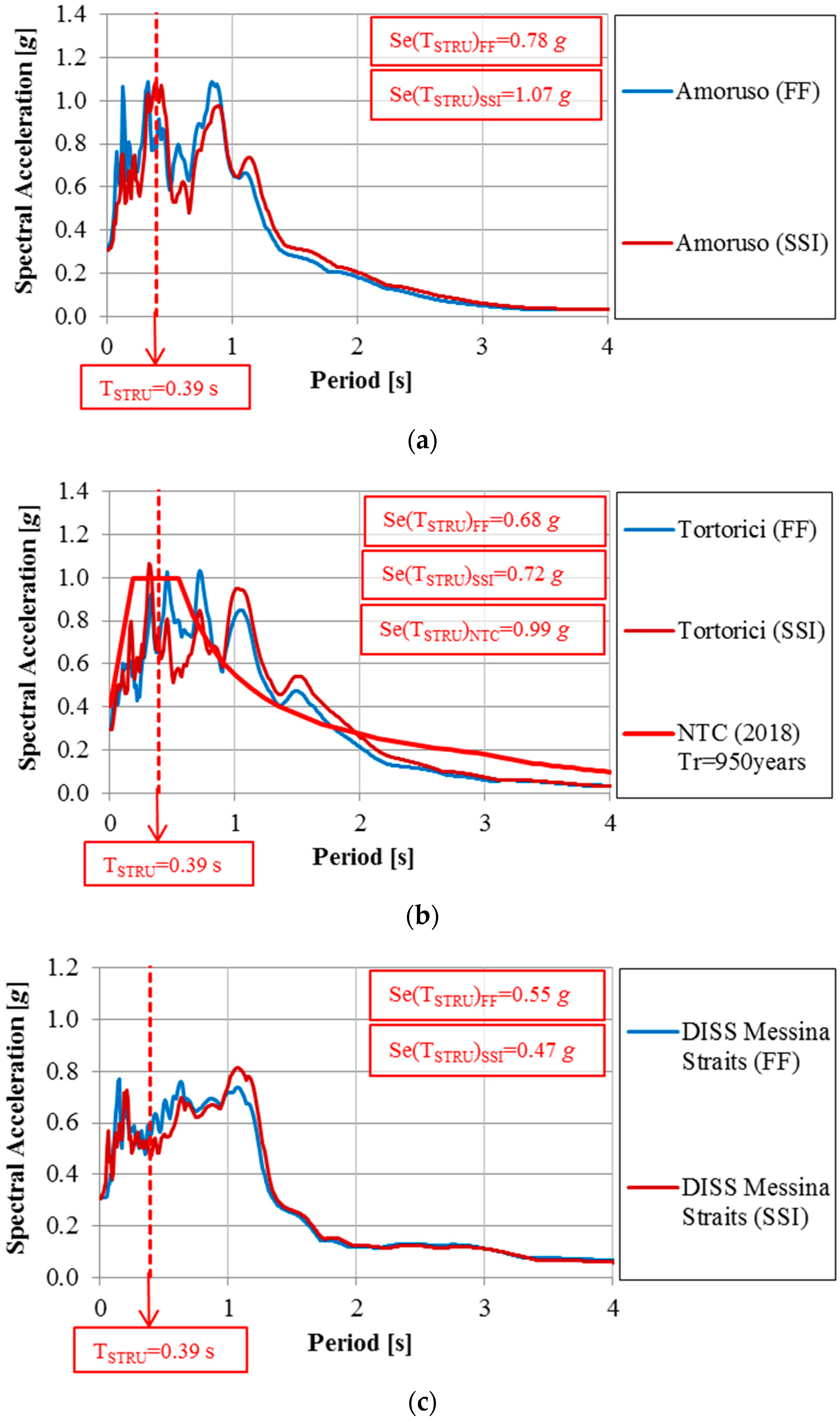
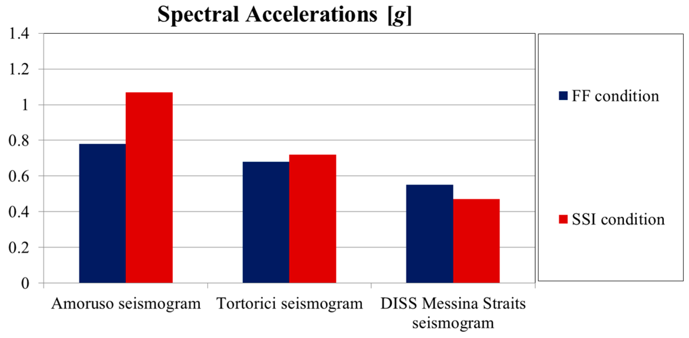
• The presence of the structure causes higher acceleration values at the foundation level. For the period of the studied structure, spectral accelerations obtained for the SSI alignment are greater than those found for the FF condition employing as seismic inputs the Amoruso and Tortorici seismograms. Moreover, in this specific case, the Italian Regulation spectrum [4] appears more conservative in comparison with the spectral acceleration obtained using the Tortorici seismogram and ensures safe operation.
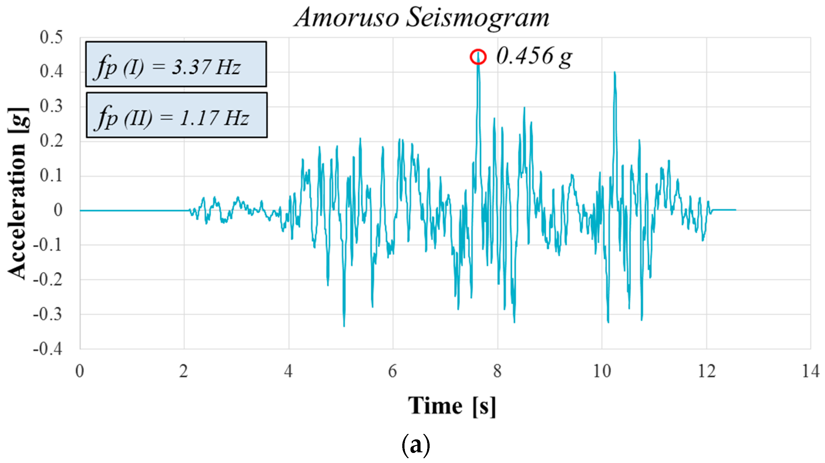
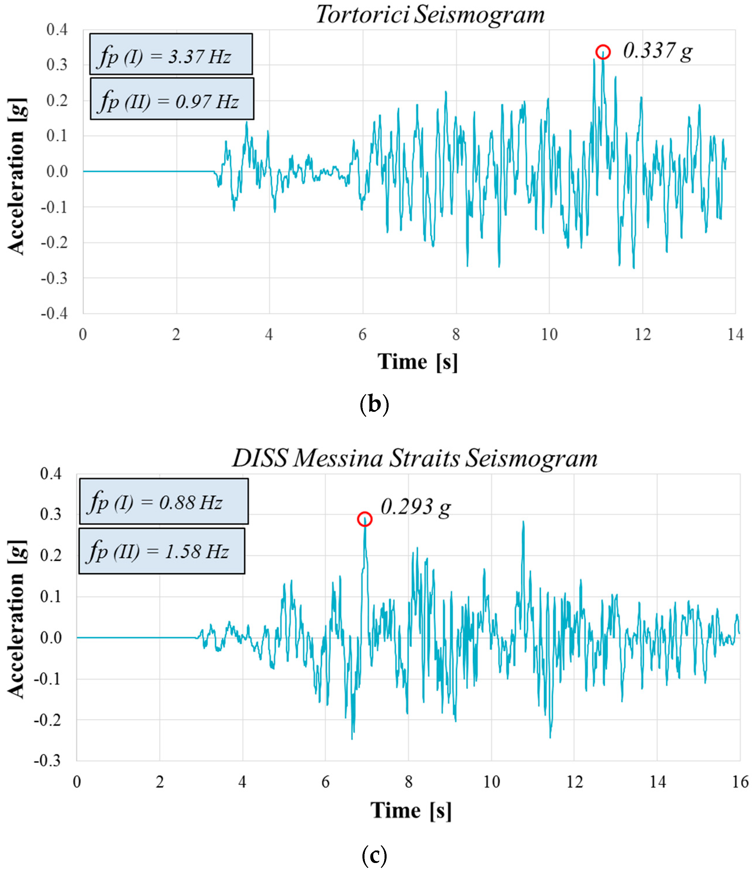
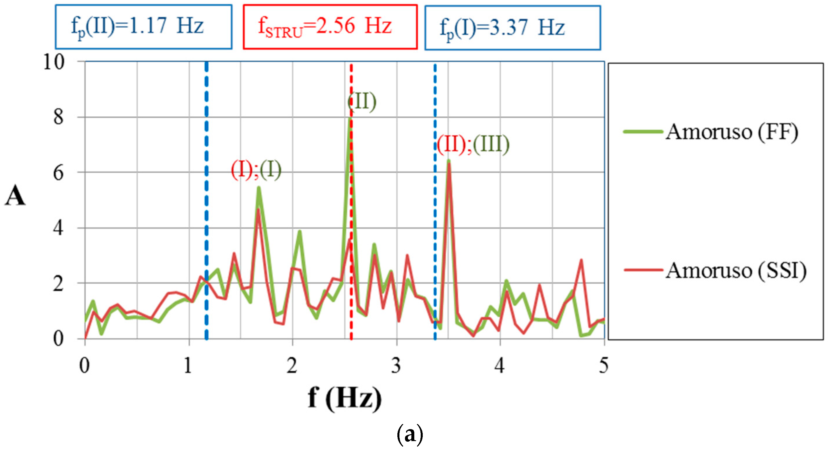
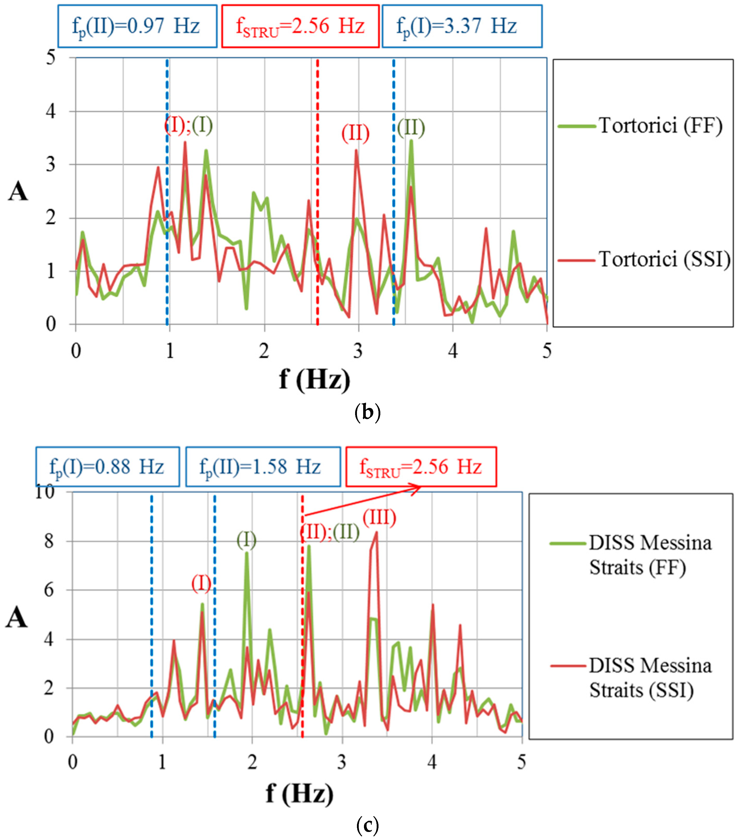
• Results in term of amplification functions, A(f), show that for the Amoruso seismogram, A(f) peaks are close to the first predominant frequency of the input motion. Moreover, the SSI has a positive effect because the second resulting frequency for the FF condition is closer to the frequency of the structure. Considering the Tortorici seismogram, the second predominant frequency of the input motion is near the first resulting frequencies, and A(f) peaks are far from the frequency of the structure. The results obtained using the DISS Messina Straits seismogram show that the first resulting frequency for the SSI condition is close to the second fundamental input frequency, and the A(f) peaks are near the frequency of the structure.
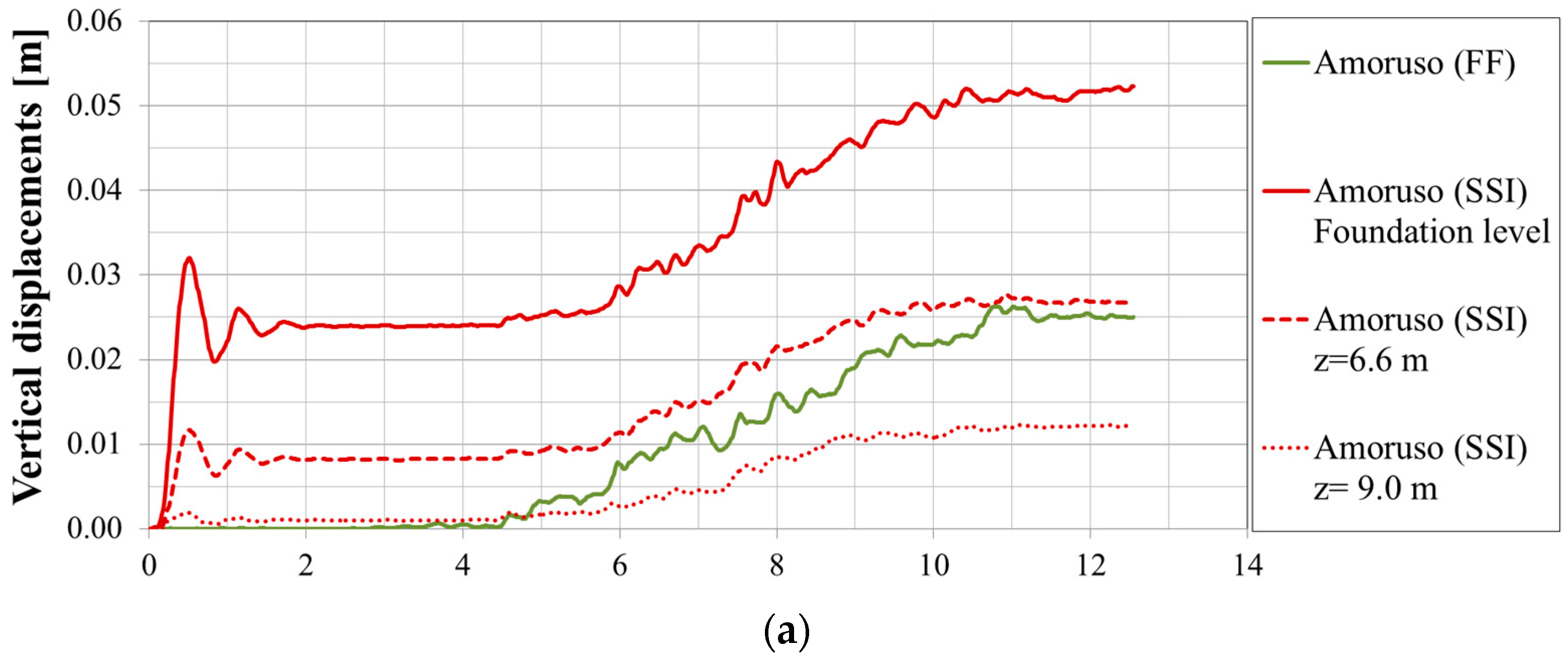
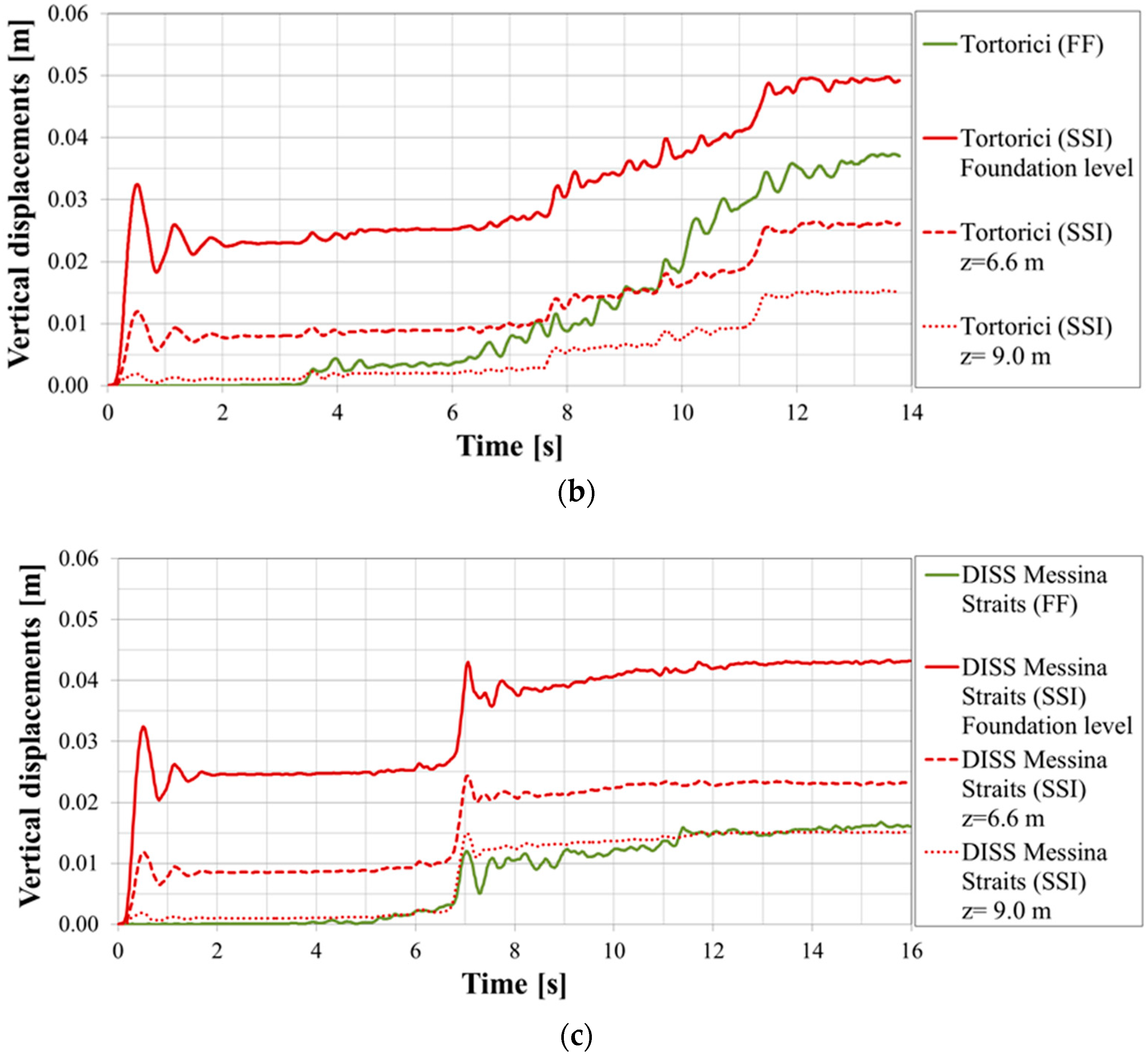
• The time histories of the settlement show that instantaneous settlements occur at the beginning of the dynamic time at the foundation level decreasing with depth along the SSI alignment, while they are zero in the FF condition. Vertical settlements reach the maximum value of about 0.05 m at the end of the dynamic time.
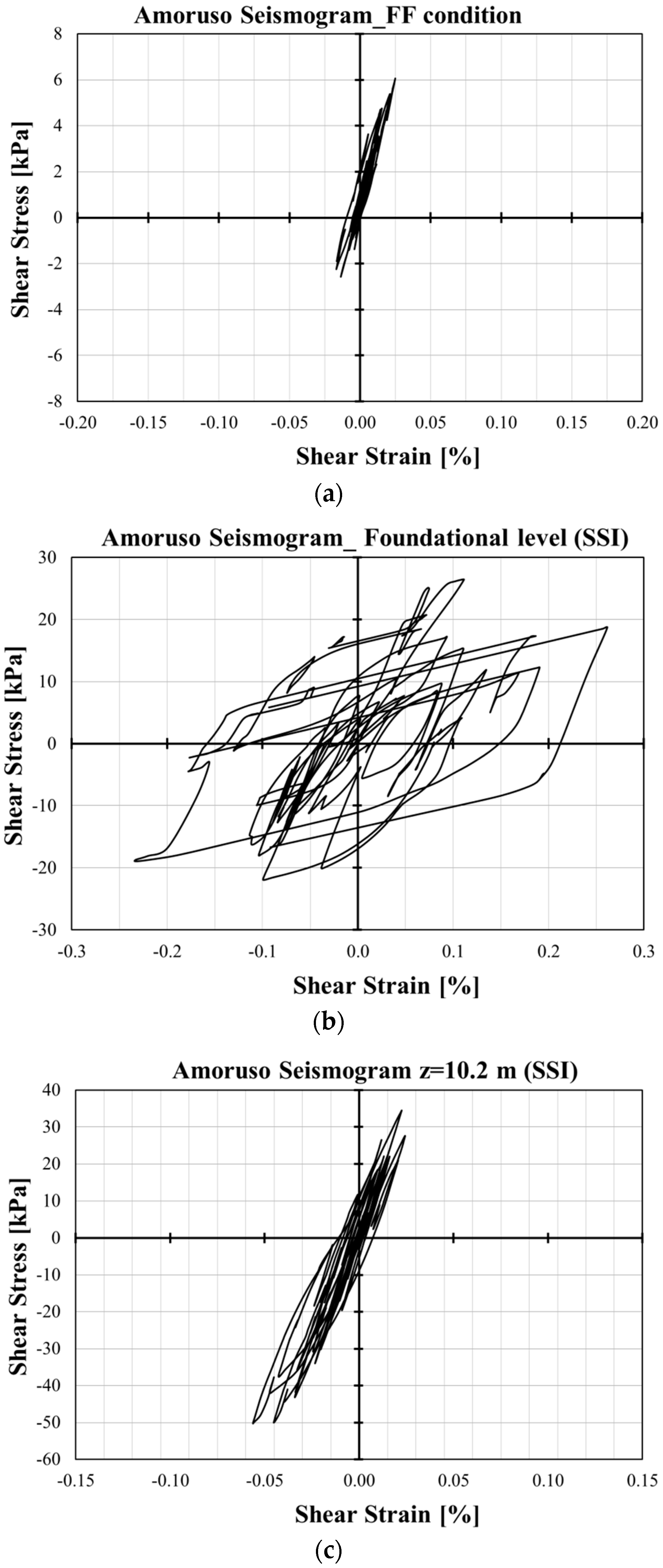
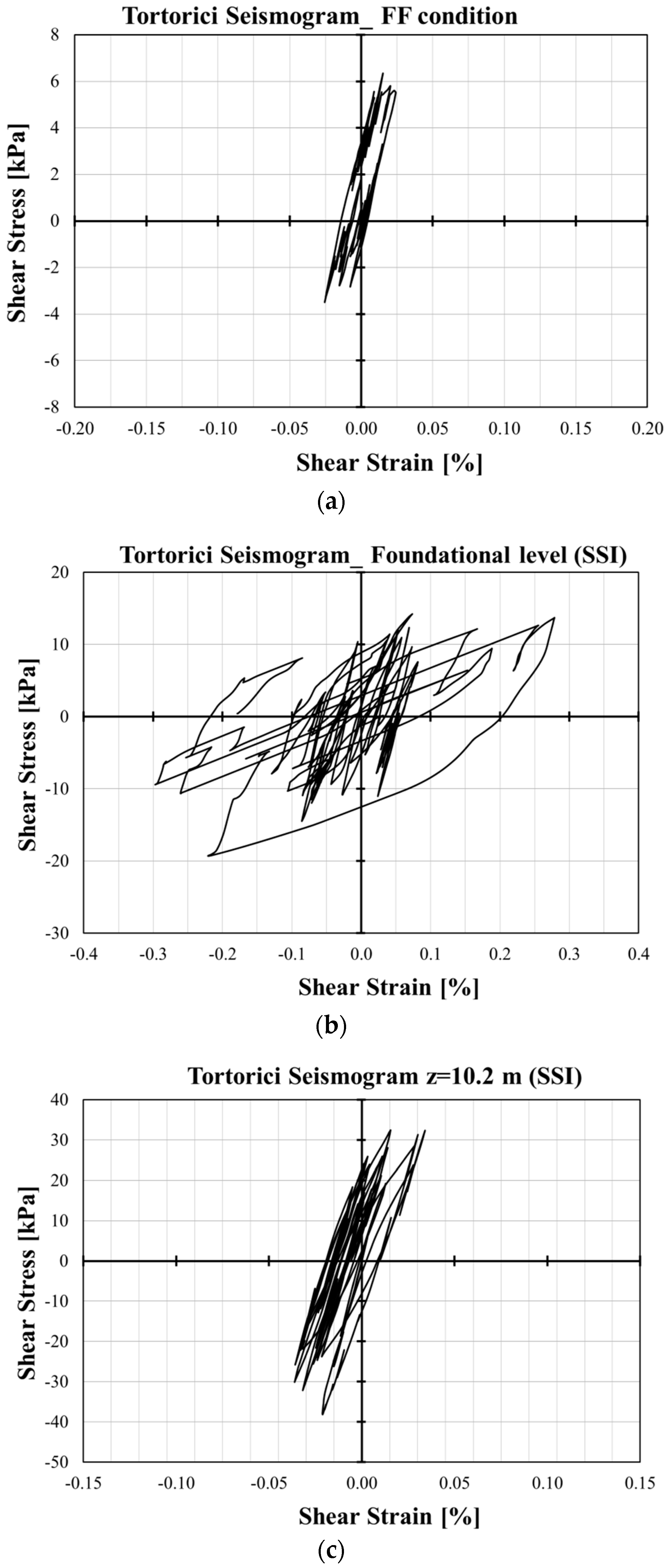
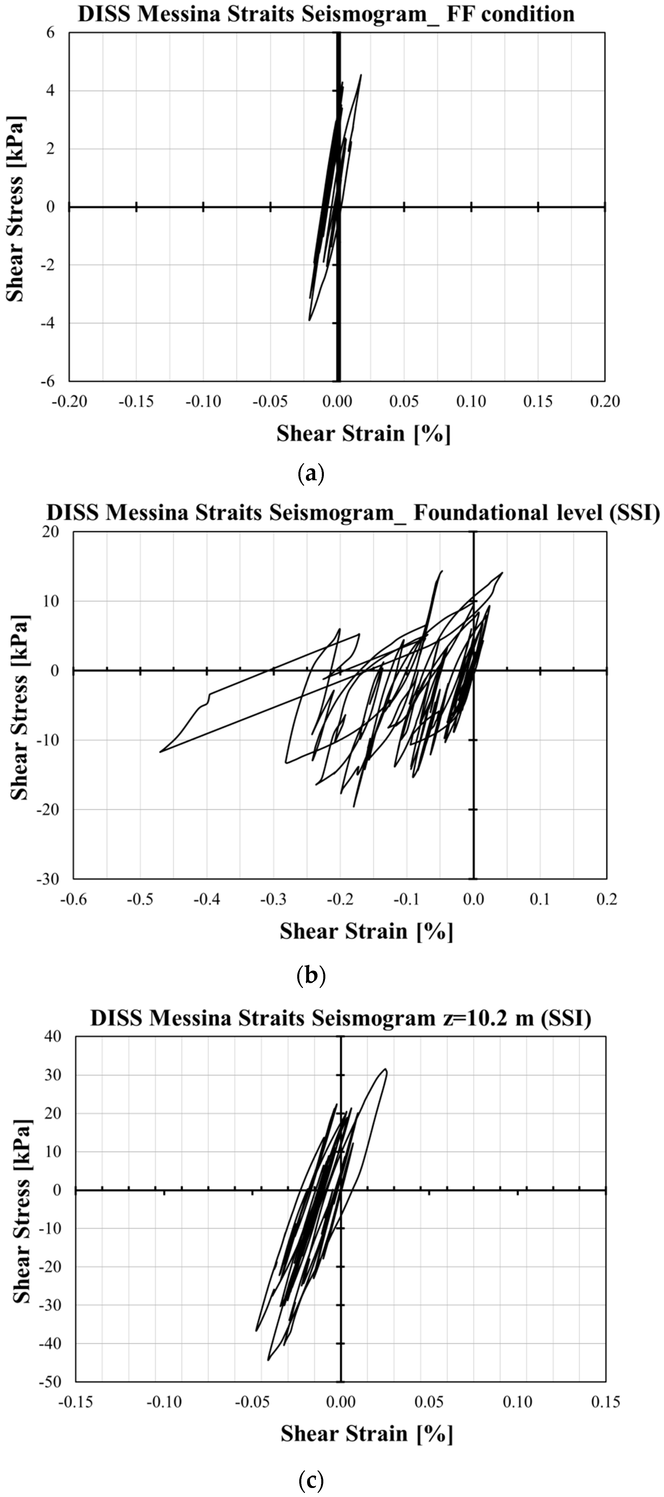
• Shear strain vs. shear stress curves show that shear stresses increase with depth, while the maximum shear strain occurs at the foundation level, exhibiting a highly nonlinear response in comparison with the FF condition. The nonlinear behavior decreases with depth along the SSI alignment.

9. Conclusions

In this paper, comparative dynamic analyses have been performed for a coupled soil–structure system to quantify SSI effects for shallow-foundation buildings. To evaluate the importance of soil nonlinearity in SSI problems, a selected set of synthetic seismograms that realistically simulate the destructive 1908 Messina and Reggio Calabria earthquake was chosen.

A deterministic approach was adopted, which is preferred in Mediterranean countries that have a moderate to high seismic risk. In particular, a parametric study was performed employing three seismograms of the 1908 earthquake corresponding to different return periods.

One crucial aspect is an accurate investigation of the soil that allows an investigation of its filtering effects in terms of acceleration and frequency. However, most studies in literature investigated nonlinear soil behavior by means of equivalent linear analyses. Instead, in this work, nonlinear analyses were carried out by employing the HS small model aimed at investigating and understanding soil hysteresis and plasticity that provide the nonlinear mechanism in the soil deposit. The HS small model was calibrated by means of several numerical simulations using experimental data derived from consolidated undrained triaxial tests, dynamic tests and geophysical tests.

Moreover, due to the kinematic and inertial interaction between the soil and the structure, the dynamic response deviates from the FF condition. Indeed, the presence of the structure can sometimes induce higher acceleration values and modify the frequency content. Therefore, a tridimensional model was developed for a strategic building in the city of Messina by means of the finite element code PLAXIS3D to describe the overall behavior of the coupled soil–structure system.

The findings reported in this study reveal the strong influence of soil nonlinearity due to the presence of the structure. The FF condition was compared with the full-coupled system to evaluate how the SSI alters the FF motion and the design accelerations. The main factors responsible for seismic motion amplification are the impedance contrast between the layers and the resonance effects due to the closeness between the predominant frequencies of the input motions and the resonance frequencies of the soil. Moreover, the matching of the resonance frequencies of the soil with the fundamental frequency of the building resting on it were also taken into account.

The results provided in this study represent valuable information for the retrofitting and/or improving of existing structures, especially in regions with medium to high seismic risk. Moreover, the investigated structure can be considered representative of the construction typology in Italy, given that most buildings in Italy were built before the 1970s, and no substantial innovations in seismic design were introduced until Law no. 64 of 2 February 1974 that made significant changes. The results reported in this work could be improved considering a visco-inelastic behavior for the structure.

References

1. Pitilakis, D.; Petridis, C. Fragility curves for existing reinforced concrete buildings, including soil–structure interaction and site amplification effects. Eng. Struct. 2022, 269, 114733. [Google Scholar] [CrossRef]
2. Vratsikidis, A.; Pitilakis, D.; Anastasiadis, A.; Kapouniaris, A. Evidence of soil-structure interaction from modular full-scale field experimental tests. Bull. Earthq. Eng. 2022, 20, 3167–3194. [Google Scholar] [CrossRef]
3. Amendola, C.; Pitilakis, D. Vulnerability assessment of historical cities including SSI and site-effects. In Proceedings of the 3rd International Issmge TC301 Symposium, Naples, Italy, 22–24 June 2022; pp. 836–846. [Google Scholar]
4. NTC [2018] D. M. 17/01/2018. New Technical Standards for Buildings. Official Journal of the Italian Republic, 2018. Available online: https://www.gazzettaufficiale.it/eli/gu/2018/02/20/42/so/8/sg/pdf (accessed on 1 December 2023).
5. Cavallaro, A.; Fiamingo, A.; Grasso, S.; Massimino, M.R.; Sammito, M.S.V. Local site amplification maps for the volcanic area of Trecastagni, south-eastern Sicily (Italy). Bull. Earthq. Eng. 2024, 22, 1635–1676. [Google Scholar] [CrossRef]
6. Cavallaro, A.; Castelli, F.; Ferraro, A.; Grasso, S.; Lentini, V. Site response analysis for the seismic improvement of a historical and monumental building: The case of Augusta Hangar. Bull. Eng. Geol. Environ. 2018, 77, 1217–1248. [Google Scholar] [CrossRef]
7. Fiamingo, A.; Bosco, M.; Massimino, M.R. The Role of Soil in Structure Response of a Building Damaged by the 26 December 2018 Earthquake in Italy. J. Rock Mech. Geotech. Eng. 2022, 15, 937–953. [Google Scholar] [CrossRef]
8. Massimino, M.R.; Abate, G.; Corsico, S.; Grasso, S.; Motta, E. Dynamic behaviour of coupled soil structure systems by means of FEM analysis for the seismic risk mitigation of INGV building in Catania (Italy). Ann. Geophys. 2018, 61, SE216. [Google Scholar] [CrossRef]
9. Oz, I.; Senel, S.M.; Palanci, M.; Kalkan, A. Effect of Soil-Structure Interaction on the Seismic Response of Existing Low and Mid-Rise RC Buildings. Appl. Sci. 2020, 10, 8357. [Google Scholar] [CrossRef]
10. Ferraro, A.; Grasso, S.; Massimino, M.R. Site effects evaluation in Catania (Italy) by means of 1-D numerical analysis. Ann. Geophys. 2018, 61, SE224. [Google Scholar] [CrossRef]
11. Seylabi, E.E.; Jeong, C.; Dashti, S.; Hushmand, A.; Taciroglu, E. Seismic response of buried reservoir structures: A comparison of numerical simulations with centrifuge experiments. Soil Dyn. Earthq. Eng. 2018, 109, 89–101. [Google Scholar] [CrossRef]
12. Schanz, T.; Vermeer, P.; Bonier, P. Formulation and verification of the Hardening Soil model. In Proceedings of the 1st International PLAXIS Symposium on Beyond 2000 in Computational Geotechnics, Rotterdam, The Netherlands, 18–20 March 1999. [Google Scholar]
13. Vakili, K.N.; Barciago, T.; Lavason, A.A.; Schanz, J. A practical approach to constitutive models for the analysis of geotechnical problems. In Proceedings of the 3rd International Conference on Computational Geomechanics (ComGeo III), Krakow, Poland, 21–23 August 2013; Volume 1. [Google Scholar]
14. Surarak, C.; Likitlersuang, S.; Wanatowski, D.; Balasubramaniam, A.; Oh, E.; Guan, H. Stiffness and strength parameters for hardening soil model of soft and stiff Bangkok clays. Soils Found. 2012, 52, 682–697. [Google Scholar] [CrossRef]
15. Benz, T. Small-Strain Stiffness of Soils and Its Numerical Consequences. Ph.D. Thesis, University of Stuttgart, Stuttgart, Germany, 2006. [Google Scholar]
16. Benz, T.; Vermeer, P.A.; Schwab, R. A small-strain overlay model. Int. J. Numer. Anal. Methods Geomech. 2009, 33, 25–44. [Google Scholar] [CrossRef]
17. Grasso, S.; Massimino, M.R.; Sammito, M.S.V. New Stress Reduction Factor for Evaluating Soil Liquefaction in the Coastal Area of Catania (Italy). Geosciences 2021, 11, 12. [Google Scholar] [CrossRef]
18. Pino, P.; D’Amico, S.; Orecchio, B.; Presti, D.; Scolaro, S.; Torre, A.; Neri, G. Integration of geological and geophysical data for re-evaluation of local seismic hazard and geological structure: The case study of Rometta, Sicily (Italy). Ann. Geophys. 2018, 61, SE227. [Google Scholar] [CrossRef]
19. Tarquini, S.; Isola, I.; Favalli, M.; Battistini, A. TINITALY, a Digital Elevation Model of Italy with a 10 Meters Cell Size (Version 1.0) [Data Set]. Istituto Nazionale di Geofisica e Vulcanologia (INGV), 2007. Available online: https://doi.org/10.13127/TINITALY/1.0 (accessed on 4 December 2023).
20. Petruzzelli, F.; Iervolino, I. NODE: A large-scale seismic risk prioritization tool for Italy based on nominal structural performance. Bull. Earthq. Eng. 2021, 19, 2763–2796. [Google Scholar] [CrossRef]
21. Lanzo, G.; Silvestri, F. Risposta Sismica Locale, 1st ed.; Helvelius: Napoli, Italy, 1999. [Google Scholar]
22. Forcellini, D. Seismic fragility of tall buildings considering soil structure interaction (SSI) effects. Structures 2022, 45, 999–1011. [Google Scholar] [CrossRef]
23. Galavi, V.; Petalas, A.; Brinkgreve, R.B.J. Finite element modelling of seismic liquefaction in soils. Geotech. Eng. J. SEAGS AGSSEA 2013, 44, 55–64. [Google Scholar]
24. PLAXIS3D, Scientific Manual. 2018. Available online: https://communities.bentley.com/products/geotech-analysis/w/plaxissoilvision-wiki/50826/manuals-archive---plaxis (accessed on 1 December 2023).
25. Joyner, W.B.; Chen, A.T.F. Calculation of non linear ground response in earthquake. Bull. Seismol. Soc. Am. 1975, 65, 1315–1336. [Google Scholar]
26. Chen, X.; Fang, P.; Chen, Q.; Hu, J.; Yao, K.; Liu, Y. Influence of cutterhead opening ratio on soil arching effect and face stability during tunnelling through non-uniform soils. Undergr. Space 2024, 17, 45–59. [Google Scholar] [CrossRef]
27. Chen, X.; Chen, P.; Liu, Y. Large-deformation finite-element analysis of square foundations in spatially variable sediments. Int. J. Geomech. 2023, 23, 8. [Google Scholar] [CrossRef]
28. Gaudio, D. Interazione Dinamica Terreno—Struttura di Pozzi di Fondazione di Pile di Ponti e Viadotti. Ph.D. Thesis, Sapienza University of Rome, Rome, Italy, 2017. Available online: https://hdl.handle.net/11573/947638 (accessed on 1 November 2023). (In Italian).
29. Bardet, J.P.; Ichii, K.; Lin, C.H. EERA: A Computer Program for Equivalent-Linear Earthquake Site Response Analyses of Layered Soil Deposits; User Manual; University of Southern California: Berkeley, CA, USA, 2000; 40p. [Google Scholar]
30. Kottke, A.R.; Rathje, E.M. Technical Manual for Strata. PEER Report. Pacific Earthquake; Engineering Research Center College of Engineering, University of California: Berkeley, CA, USA, 2008. [Google Scholar]
31. Mejia, L.H.; Dawson, E.M. Earthquake Deconvolution for FLAC. In Proceedings of the 4th International FLAC Symposium on Numerical Modeling in Geomechanics, Madrid, Spain, 29–31 May 2006; Itasca Consulting Group: Minneapolis, MN, USA, 2006. [Google Scholar]
32. Amoruso, A.; Crescentini, L.; Scarpa, R. Source parameters of the 1908 Messina Straits, Italy, earthquake from geodetic and seismic data. J. Geophys. Res. 2002, 107, ESE-4–ESE-11. [Google Scholar] [CrossRef]
33. Tortorici, L.; Monaco, C.; Tansi, C.; Cocina, O. Recent and active tectonics in the Calabrian arc (Southern Italy). Tectonophysics 1995, 243, 37–55. [Google Scholar] [CrossRef]
34. Basili, R.; Valensise, G.; Vannoli, P.; Burrato, P.; Fracassi, U.; Mariano, S.; Tiberti, M.M.; Boschi, E. The Database of Individual Seismogenic Sources (DISS), version 3: Summarizing 20 years of research on Italy’s earthquake geology. Tectonophysics 2008, 453, 20–43. [Google Scholar] [CrossRef]
35. Valensise, G.; Pantosti, D. A 125 Kyr-long geological record of seismic source repeatability: The Messina Straits (southern Italy) and the 1908 earthquake (Ms=7.5). Terra Nova 1992, 4, 472–483. [Google Scholar] [CrossRef]
36. Brinkgreve, R.B.J.; Kappert, M.H.; Bonnier, P.G. Hysteretic damping in a small-strain stiffness model. In Proceedings of the Tenth International Symposium on Numerical Models in Geomechanics (NUMOG X), Rhodes, Greece, 25–27 April 2007; pp. 737–742. [Google Scholar]
37. Massimino, M.R.; Abate, G.; Corsico, S.; Louarn, R. Comparison Between Two Approaches for Non-linear FEM Modelling of the Seismic Behaviour of a Coupled Soil–Structure System. Geotech. Geol. Eng. 2019, 37, 1957–1975. [Google Scholar] [CrossRef]
Figure 1. (a) Overview of the study area with the location of field tests: Seismic Dilatometer Marchetti Test (SDMT) and S1, S2 and S3 boreholes; (b) SE and (c) NE views of the DPRC (From Tarquini et al. [19]; Google Maps, modified).
Geosciences 14 00100 g001
Figure 2. Plan view (raised floor) of the building.
Geosciences 14 00100 g002
Figure 3. (a) 3D view and (b) axonometric cross section.
Geosciences 14 00100 g003
Figure 4. (a) Double flat jack test performed on the masonry walls; (b) foundation inspection pit.
Geosciences 14 00100 g004
Figure 5. (a) Shear wave velocity, VS, profiles derived from the down-hole test (S3 borehole), cross-hole test (S1 and S2 boreholes) and Seismic Dilatometer Marchetti test (SMDT); (b) soil stratigraphy obtained from the S3 borehole.
Geosciences 14 00100 g005
Figure 6. Deviator stress–axial strain relationships under different effective consolidation pressures for a back pressure of 190 kPa (sample S3C4).
Geosciences 14 00100 g006
Figure 7. (a) G/G0 versus γ [%] curves; (b) ξ [%] versus γ [%] curves (samples S1C1 and S3C4).
Geosciences 14 00100 g007
Figure 8. Soil stratigraphy obtained from in situ characterization.
Geosciences 14 00100 g008
Figure 9. Model geometry with the indication of the free-field (FF) and soil–structure interaction (SSI) conditions.
Geosciences 14 00100 g009
Figure 10. Finite element mesh of the coupled soil–structure system.
Geosciences 14 00100 g010
Figure 11. Seismic inputs with the indication of the first and second predominant frequencies (fp): (a) Amoruso, (b) Tortorici and (c) DISS Messina Straits seismograms. The red circles indicate the PGA values.
Geosciences 14 00100 g011aGeosciences 14 00100 g011b
Figure 12. Comparison between the calibrated model and the results of CUTxT for sample S3C4 under different values of p′c: (a) 200 kPa; (b) 400 kPa; (c) 600 kPa.
Geosciences 14 00100 g012aGeosciences 14 00100 g012b
Figure 13. Comparison between the calibrated model and the results of the CLTST performed on sample S3C4. The dashed-line portion of the black curve indicates the value of the unloading–reloading stiffness, Gur, that limits the tangent shear modulus, Gt. Intersecting dotted black lines indicate the shear strain level, γ0.7, at which the secant shear modulus, GS, is reduced to 72.2% of G0.
Geosciences 14 00100 g013
Figure 14. Damping ratio as a function of the cyclic shear strain in the HS small model compared with the results of the CLTST performed on sample S3C4. The vertical dotted black line represents the cut-off shear strain.
Geosciences 14 00100 g014
Figure 15. Maximum accelerations with depth along SSI and FF alignments using: (a) Amoruso, (b) Tortorici and (c) DISS Messina Straits seismograms.
Geosciences 14 00100 g015
Figure 16. Results at the surface in terms of spectral accelerations using: (a) Amoruso, (b) Tortorici and (c) DISS Messina Straits seismograms.
Geosciences 14 00100 g016
Figure 17. Comparison between the spectral accelerations for the period of the structure using the three 1908 synthetic seismograms.
Geosciences 14 00100 g017
Figure 18. Amplification functions, A(f), for FF and SSI conditions using: (a) Amoruso, (b) Tortorici and (c) DISS Messina Straits seismograms.
Geosciences 14 00100 g018aGeosciences 14 00100 g018b
Figure 19. Deformed mesh (scaled up 30 times) obtained at the end of the dynamic phase for the Amoruso seismogram.
Geosciences 14 00100 g019
Figure 20. Comparison between the vertical displacements for the FF and SSI conditions using: (a) Amoruso, (b) Tortorici and (c) DISS Messina Straits seismograms.
Geosciences 14 00100 g020aGeosciences 14 00100 g020b
Figure 21. Stress–strain hysteretic loops obtained using the Amoruso seismogram: (a) for the FF condition; (b) for the SSI condition at the foundation level and (c) at a depth of 10.2 m.
Geosciences 14 00100 g021
Figure 22. Stress–strain hysteretic loops obtained using the Tortorici seismogram: (a) for the FF condition; (b) for the SSI condition at the foundation level and (c) at a depth of 10.2 m.
Geosciences 14 00100 g022
Figure 23. Stress–strain hysteretic loops obtained using the DISS Messina Straits seismogram: (a) for the FF condition; (b) for the SSI condition at the foundation level and (c) at a depth of 10.2 m.
Geosciences 14 00100 g023