Article

Mapping Seafloor Sediment Distributions Using Public Geospatial Data and Machine Learning to Support Regional Offshore Renewable Energy Development

by
Connor W. Capizzano
1,*,
Alexandria C. Rhoads
1,
Jennifer A. Croteau
1,
Benjamin G. Taylor
1,
Marisa L. Guarinello
1,* and
Emily J. Shumchenia
2
1
INSPIRE Environmental Inc., 513 Broadway, Suite 314, Newport, RI 02840, USA
2
Northeast Regional Ocean Council, 50 F Street NW, Suite 750, Washington, DC 20001, USA
*
Authors to whom correspondence should be addressed.
Geosciences 2024, 14(7), 186; https://doi.org/10.3390/geosciences14070186
Submission received: 1 June 2024 / Revised: 26 June 2024 / Accepted: 4 July 2024 / Published: 11 July 2024
(This article belongs to the Special Issue Progress in Seafloor Mapping)

Abstract

:
Given the rapid expansion of offshore wind development in the United States (US), the accurate mapping of benthic habitats, specifically surficial sediments, is essential for mitigating potential impacts on these valuable ecosystems. However, offshore wind development has outpaced results from environmental monitoring efforts, compelling stakeholders to rely on a limited set of public geospatial data for conducting impact assessments. The present study therefore sought to develop and evaluate a systematic workflow for generating regional-scale sediment maps using public geospatial data that may pose integration and modeling challenges. To demonstrate this approach, sediment distributions were characterized on the northeastern US continental shelf where offshore wind development has occurred since 2016. Publicly available sediment and bathymetric data in the region were processed using national classification standards and spatial tools, respectively, and integrated using a machine learning algorithm to predict sediment occurrence. Overall, this approach and the generated sediment composite effectively predicted sediment distributions in coastal areas but underperformed in offshore areas where data were either scarce or of poor quality. Despite these shortcomings, this study builds on benthic habitat mapping efforts and highlights the need for regional collaboration to standardize seafloor data collection and sharing activities for supporting offshore wind energy decisions.

1. Introduction

Offshore wind is widely recognized as a valuable source of clean and renewable energy for addressing energy demands and climate change impacts [1,2]. In the United States (US), the Biden–Harris Administration set an ambitious goal of deploying 30 gigawatts (GW) of offshore wind energy capacity by 2030 and establish a pathway to deploying at least 110 GW by 2050 to strengthen energy security and reduce carbon emissions [3]. Since the first commercial offshore wind farm became operational in 2016, the US has made significant strides in the development of commercial offshore wind energy projects to decrease fossil fuel dependency, limit carbon emissions, and mitigate climate change impacts. However, while driven by the desire to mitigate climate change, offshore wind technology and construction processes are relatively novel and there is growing concern among ocean user groups about potential impacts on marine ecosystems. With a potential generating capacity of over 50 GW across 32 active lease developments in the US offshore wind energy project pipeline to date [4,5], there is a significant need to understand these interactions to avoid, minimize, and mitigate adverse impacts and ensure coexistence of offshore wind development with marine ecosystems and the communities they support [6].
While observed to exert pressure on various ecological [7] and socio-economic systems [8], all offshore wind development activities will interact with and potentially alter the seafloor and its benthic ecosystems. Marine benthic habitats are physically distinct areas of seabed that provide essential resources, such as space for shelter, feeding, and reproduction, to the biological communities that are associated with them [9]. Structurally complex habitats, including natural hard bottom environments composed of gravel, cobble, and boulder substrates, are particularly valuable to the regions they occupy as they directly and indirectly support a variety of ecosystems services that benefit ecological processes and society [10,11,12]. However, habitat disturbances and losses can cause significant changes in species richness and abundance [13,14] and are expected to be increasingly dominant threats to marine wildlife [15]. Even in instances where a habitat is not lost but altered, like with the introduction of new habitats from offshore wind infrastructure, ecosystem structure and functioning can be impacted [16,17]. Given the rapid expansion of offshore wind planning into new areas on the US outer continental shelf, understanding the distribution of benthic habitats over large areas is fundamental to the long-term sustainability of these benthic ecosystems and the communities they support.
Mapping the distribution of benthic habitats, particularly surficial sediments, is a challenging task due to the availability and coverage of environmental data [18]. Benthic habitats are inherently variable as they are influenced by a variety of physical, chemical, and biological elements over multiple temporal and spatial scales that make it difficult to sample and obtain comprehensive geospatial datasets for analysis [19]. Direct sediment or in situ sampling field efforts provide detailed sediment information for the small portion of seafloor that they sample. However, these methods are typically costly in terms of effort and financial investment and make it difficult to accurately represent seafloor characteristics over broad areas [19,20]. Acoustic remote sensing methods, in contrast, collect wide swaths of seafloor information and can effectively map an entire study area [21,22,23,24]. Multi-beam echosounders, for instance, can simultaneously collect bathymetric and backscatter data, which have been used effectively to interpret sediment distributions by identifying seafloor features with geologic relevance [22,25] and seafloor physical properties [26], respectively. Yet, characterizing seafloor sediment types from remote sensing data requires the integration of direct sampling or “ground truth” information to derive geologically meaningful maps, which have been reviewed by [19].
With the dramatic increase in digital data, computational processing, and spatial analysis software, there are now a variety of modern approaches for integrating sediment information from direct sampling and remotely sensed environmental datasets to accurately map benthic sediment distributions. Supervised empirical models, including regression and generalized models and classifiers, have been broadly adopted over the last decade due to their predictive performance and objectivity for producing habitat maps, as reviewed by [19]. In comparison to manual interpretation methods, supervised empirical models identify statistical relationships between ground truth sediment samples (response variable) and environmental data at sampling locations (explanatory variables), allowing for the prediction of sediment types at unsampled locations and generation of full-coverage maps when coupled with continuous environmental data [27]. However, the validity and predictive accuracy of empirical models depend on how well data meet underlying model assumptions [28], which is challenging when working with data collected from complex benthic ecosystems. Consequently, more automated machine learning algorithms, including random forests, maximum entropy, and clustering techniques, are being favored due to their ability to model complex and nonlinear relationships without needing to satisfy restrictive assumptions required by empirical models [29]. Such approaches can explain and predict ecological patterns with high accuracy [29] and have shown great promise when mapping the distribution of benthic habitats [27,30,31,32,33].
Despite these technological and analytical advancements, most of the ocean floor remains unmapped and unexplored [34]. To complicate matters further, offshore wind development has progressed faster than the establishment of monitoring plans that gather sediment distribution data and objectively contextualize potential impacts. Proactive siting and pre-construction impact assessments therefore often capitalize on in situ sediment observations and remotely sensed environmental data from online public repositories to guide decision-making activities. However, differences in mapping objectives, the introduction of new technologies over time, and lack of technical processing standards have resulted in an assortment of seafloor data that not only vary by coverage but also type and quality. For instance, despite the value of backscatter information for interpreting seafloor substrates and benthic habitats [22,26], current global seafloor mapping efforts focus primarily on acquiring bathymetry over a range of resolutions [35]. Reported metrics for in situ sediment observations can also vary depending on sampling method, ranging from quantitative measures (e.g., grain size) to more qualitative classifications (e.g., sediment type). Such differences and gaps can prevent the integration of mutually exclusive datasets and effectively interfere with the transfer of knowledge for evaluating complex processes [36].
Given the ever increasing need to understand baseline conditions to inform offshore wind development activities, the development of objective, quantitative, and repeatable workflows with seafloor information from public repositories is vital for making environmentally sustainable decisions in a timely manner. To this end, the overall goal of this study was to develop and evaluate a standardized approach for generating comprehensive and regional-scale sediment maps using publicly accessible data that may pose integration and modeling challenges. This study specifically sought to illustrate the utility of national classification standards and spatial analysis tools for establishing consistent data structures and machine learning algorithms and other statistics for modeling complex, non-linear relationships and making objective decisions. The results of this study will establish recommendations for pursuing similar desktop-based mapping efforts to inform stakeholders invested in project-specific and regional scale offshore energy development.

2. Materials and Methods
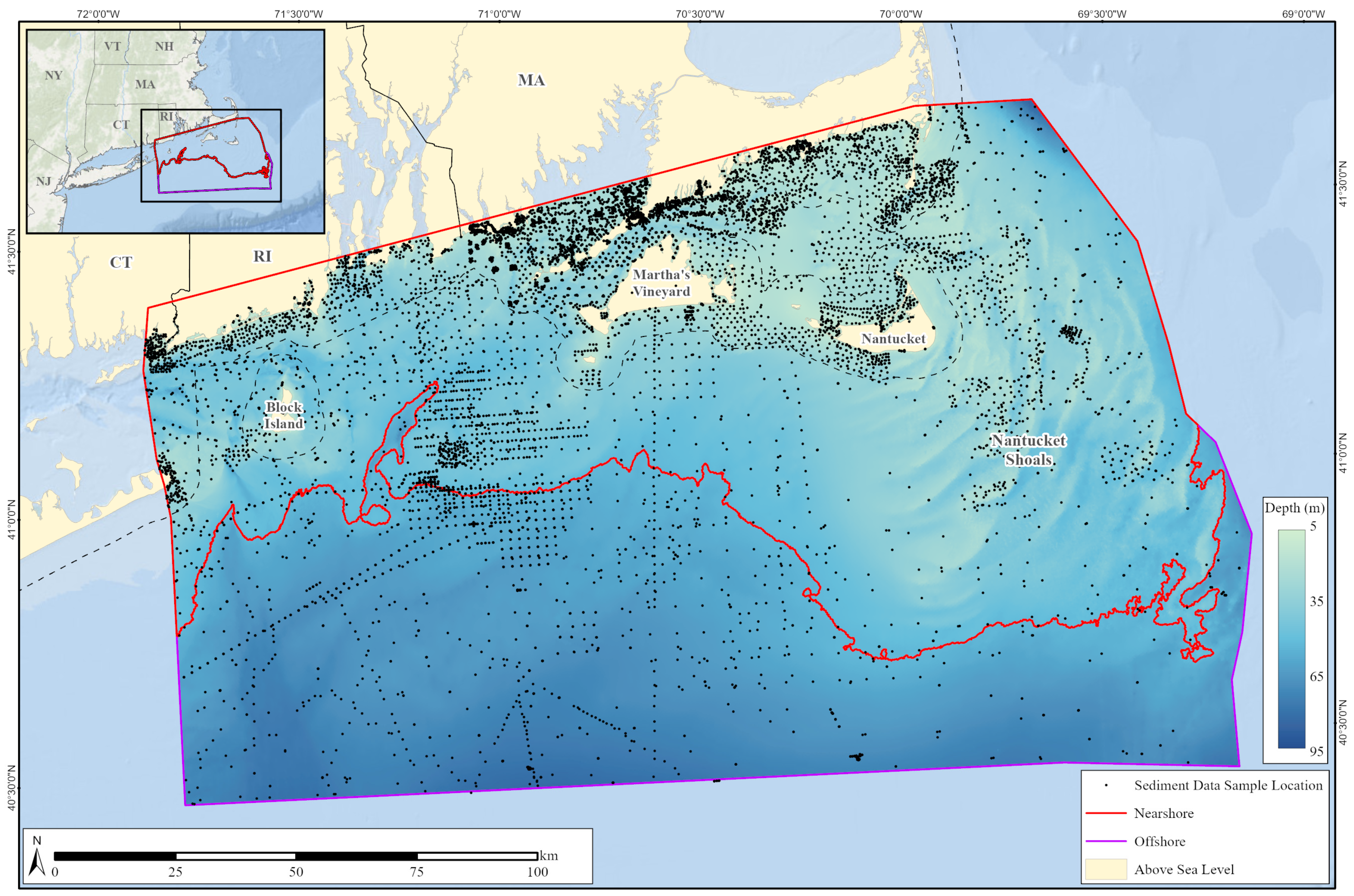
2.1. Study Area

To demonstrate our methodology, we characterized sediment distributions on the northeastern U.S. continental shelf, specifically off the coast of southern New England between Long Island, New York and Nantucket Island, Massachusetts (Figure 1). The study area includes over 3100 square kilometers (km2) of continental shelf gently sloping to depths of 95 m and encompasses features such as Rhode Island Sound, Nantucket Sound, and the Nantucket Shoals. Sand is the predominant surficial sediment type on the shelf with small, localized areas of sand–shell and sand–gravel. Fine sediments are also common in the study area off southern New England, where tidal currents slow significantly and allow silts and clays to settle out and mix with sand [37]. Hard bottom habitats consisting of gravel, cobble, or boulders, while limited in their spatial distribution over this region, are known to support a diverse and abundant assemblage of economically important resources, including American lobsters (Homarus americanus) [38], longfin squid (Loligo pealei) [39,40], and Atlantic cod (Gadus morhua) [41].
Given the predominance of bathymetric resources both globally [34] and in this region [42] over other remotely sensed environmental data, we only considered bathymetric data in this study to demonstrate spatial processing and modeling challenges that could be encountered in other regions. Preliminary investigations of publicly available geospatial data also indicated sediment sample locations and bathymetric features occurred more frequently in shallow areas on the continental shelf. Therefore, to increase confidence in outputs from the modeling approach, we divided the study area into two subareas (i.e., “nearshore” and “offshore”) using the 45 m bathymetric contour.

2.2. Data Collection and Formatting

A desktop study was conducted to collect and evaluate the suitability of existing and publicly accessible geospatial datasets within the designated study area. Regional in situ sediment observations and bathymetric raster data were collected from various public sources, including those hosted by federal agencies (e.g., Bureau of Ocean Energy Management, US Geological Survey [USGS], National Oceanic and Atmosphere Administration), academic institutions, and non-governmental organizations. Data from the Bureau of Ocean Energy Management also included sediment observations listed in site assessment and characterization reports from recent offshore wind activities in the study area. Search queries were limited to georeferenced (i.e., spatially defined) datasets across all study years to maximize sediment observations and bathymetric data coverage over the study area. Tabular sediment observation records were preferred over other popular geospatial file types (e.g., vector polygons, raster imagery) to exclude interpolated sediment results. Given that no laboratory analyses were anticipated to further process sediment field data (e.g., text extractions, review of towed video data), only sediment observation records with grain size estimates and other quantitative information were considered. As mentioned previously, only bathymetry raster data were considered due to their availability over other seafloor data types (e.g., backscatter) and ability to provide continuous environmental data throughout the study area.
In brief, a total of twelve geospatial datasets, including nine sediment datasets and three bathymetric datasets, were found on websites hosted by federal and state agencies and non-profit organizations. In situ sediment observations (n = 11,744) were primarily sourced from the USGS US Seafloor Sediment Database (usSEABED), USGS East-Coast Sediment Texture Database, and directed benthic assessments for select areas off southern New England, including efforts within offshore wind development areas. The usSEABED and East-Coast Sediment Texture databases are comprehensive repositories of sediment texture data from numerous marine sampling programs over several decades. Consequently, sediment records were collected primarily between 1930 and 2020 with some records dating back to 1842 (Supplementary Figure S1) and sampled with a variety of sediment sampling (e.g., sediment grabs, cores) and underwater imagery (e.g., sediment profile imaging, plan view imaging, drop-camera, and towed video) methods. Bathymetric data products were available from data repositories hosted by federal agencies (i.e., USGS) and non-profit organizations (i.e., The Nature Conservancy). These products ranged from 2-m to 250-m in resolution and were compiled using acoustic remote sensing data primarily collected in the early 21st century (2001–2015) and extending as far back as 1851. Sediment observations and bathymetric data products were provided in a variety of file formats for ingestion and processing, including spreadsheets, geospatial features, and printed tables in reports for sediment datasets and software-specific raster files for bathymetric data products. Additional metadata for each sediment and bathymetric dataset are available in Supplementary Table S1.
Collected geospatial data were then processed accordingly to ensure data structures were consistent for anticipated modeling routines. In situ sediment observations, for instance, were reclassified into Substrate Group and Substrate Subgroup sediment classifications defined by the Coastal and Marine Ecological Classification Standard (CMECS), a US-based framework for classifying and describing coastal and marine ecosystems [43]. Sediment results presented as grain sizes were converted to these CMECS sediment classes using grain size descriptor crosswalks (Table 1) [43,44]. CMECS sediment class definitions were also used to reclassify in situ sediment observations presented as proportions of each major Substrate Group. Given the number of Substrate Group and Substrate Subgroup combinations, CMECS sediment groupings were used to generalize in situ sediment observations into five “determined sediment classes”, specifically Gravel (n = 1178), Gravel Mixes (n = 613), Gravelly (n = 413), Sand (n = 6358), and Sand–Mud Mix (n = 3182), to reduce complexity.
Bathymetric data were processed and reviewed to ensure available data provided full coverage of the study area. High-resolution geophysical raster data (i.e., 2-m resolution, NOAA National Ocean Service) were down-sampled to a minimum resolution of 8-m to balance the competing needs of data quality and computational performance. Preliminary investigations confirmed that a decrease from the initially targeted 4 m to 8 m resolution reduced computing time and preserved patterns in predicted results (Supplementary Figure S2). Processed geophysical raster data were finally merged into a single mosaic dataset (that varied in resolution depending on the final source data) to provide continuous environmental data over the study area for subsequent modeling. Given that mosaic datasets retain the resolution of input raster data, the resolution of the generated mosaic dataset ranged from 8 to 250 m.

2.3. Data Analysis

A systematic workflow was developed to produce a habitat delineation data product from sediment observations and bathymetric data (Figure 2). This protocol consisted of the following steps:
  • Selection of explanatory and response variables from the collected datasets;
  • Evaluation of bathymetric characteristics for predicting the presence of individual sediment types (i.e., classes);
  • Generation of a sediment presence composite map from individual sediment class predictions.
Geospatial data processing and variable extraction were conducted using Esri’s ArcGIS software suite (version 10.8.2) and the Benthic Terrain Modeler extension [45], which requires the Spatial Analyst extension. Statistical analyses were performed with the computing software R (version 4.1.3) [46] and the packages “dismo” (version 1.3-5) [47] and “rJava” (version 1.0-6) [48].

2.3.1. Variable Preparation

Sediment observations and bathymetric data were further processed to identify appropriate variables for properly modeling the influence of bathymetric characteristics on sediment-type presence. A set of explanatory variables were initially considered and extracted from the bathymetric mosaic dataset described previously using the Benthic Terrain Modeler extension in Esri’s ArcGIS software suite (version 10.8.2) (Table 2). Pearson correlation coefficients were calculated to measure the strength and direction of linear relationships between pairs of these explanatory variables, where highly correlated variables (r > 0.6) were removed to limit model multicollinearity (Figure 3). In the end, seven of the nine explanatory variables were retained from the bathymetric mosaic dataset to predict the presence of benthic sediments. These seven variables included depth, slope, aspect in both north–south and east–west components, plan (positive values, convergence) and profile (positive values, divergence) curvatures, and fine-scale bathymetric position index (inner radius of 8 m and outer radius of 25 m) (Table 2).

2.3.2. MaxEnt Modeling

While many approaches exist for modeling the geographic occurrence of a given species or feature, like sediment class, the type of model used depends heavily on what kind of data are available. The publicly available datasets collected for this study, for instance, only specify the locations where a sediment type was observed (i.e., presence-only) and rarely specify absence. Because the intent and methods for collecting these data are rarely known, presence-only data lack explicit information needed to infer the absence of sediment types, and such inferences would contain errors and biases [49].
As such, presence-only modeling has received great attention in recent years as models have continually developed to address such concerns. Maximum entropy (MaxEnt) modeling, in particular, is an increasingly popular and powerful presence-only approach that consistently competes with the top performing methods in terms of predictive performance [49,50]. MaxEnt modeling estimates the occurrence likelihood of a feature (e.g., sediment type) in space by finding the maximum entropy probability distribution, or the most uniform distribution, given a set of constraints (e.g., bathymetric characteristics) over the area of interest. In other words, this machine learning approach can estimate the distribution of a species or habitat across geographic areas without making any assumptions of what is not known [51]. Although traditionally used to model species distributions, MaxEnt modeling has been successful in mapping benthic sediments [30] and vulnerable marine ecosystems including deep sea coral habitats [52,53].
For these reasons, MaxEnt modeling was used to predict the likelihood of each sediment class occurring as a function of bathymetric characteristics within the study area. When using MaxEnt modeling, as with other machine learning approaches, to make accurate predictions, background data are separated into “training” and “test” datasets to prevent overfitting where the model cannot generalize patterns beyond the provided data and can cause inaccurate predictions on new, unseen data. The training dataset typically comprises a larger portion (70–80%) of available data and is used to teach machine learning models patterns and relationships based on known outcomes. The test dataset constitutes the remaining 20–30% of the available data and is employed to validate the predictive performance of these models on new data and identify and mitigate overfitting. Independent MaxEnt models were therefore generated for each sediment class using a randomized training dataset (70% of presence-only data; Supplementary Table S2) and the seven bathymetric variables identified previously (Table 2). Model building protocols resulted in five sediment occurrence models as well as post hoc assessments to evaluate variable importance (i.e., the predictive importance of each variable) and response (i.e., how variables affect model predictions).
The performance of each model was then evaluated to determine how often a model was truly correct or incorrect in their prediction and how often it was false in the prediction (i.e., false positives and false negatives). Several model performance metrics were calculated using a 2 × 2 confusion matrix generated from a randomized test dataset (30% of the remaining presence-only data; Supplementary Table S2), a set of randomly generated pseudo-absences, and the model output from each sediment class. One such model performance metric included assessing variation among the independent runs using the area under curve (AUC) value from the receiver-operating characteristic curves (ROCs), which measures the ability of the model to discriminate between a sediment class being present or absent on a scale from 0 to 1 [54]. An AUC value of 0.5 is considered poor predictive performance (i.e., the model predicts outcomes no better than random), 0.7 to 0.8 is acceptable, 0.8 to 0.9 is excellent, and 0.9 and greater is outstanding, as reviewed by [55]. Additional model performance metrics were calculated from the model specific confusion matrix to evaluate a model’s performance (i.e., accuracy, sensitivity [true positive rate], specificity [true negative rate], F1 score) in predicting sediment occurrence in each grid cell.
Model uncertainty in occurrence data was also estimated by comparing model prediction variation (standard deviation) between the randomly partitioned test datasets, essentially quantifying where sediment occurrence data disagreed with prediction outputs (i.e., high levels of uncertainty equal more disagreement). The test set was also used to calculate model threshold values for binary classification (see Section 2.3.3—Sediment Composite for details).

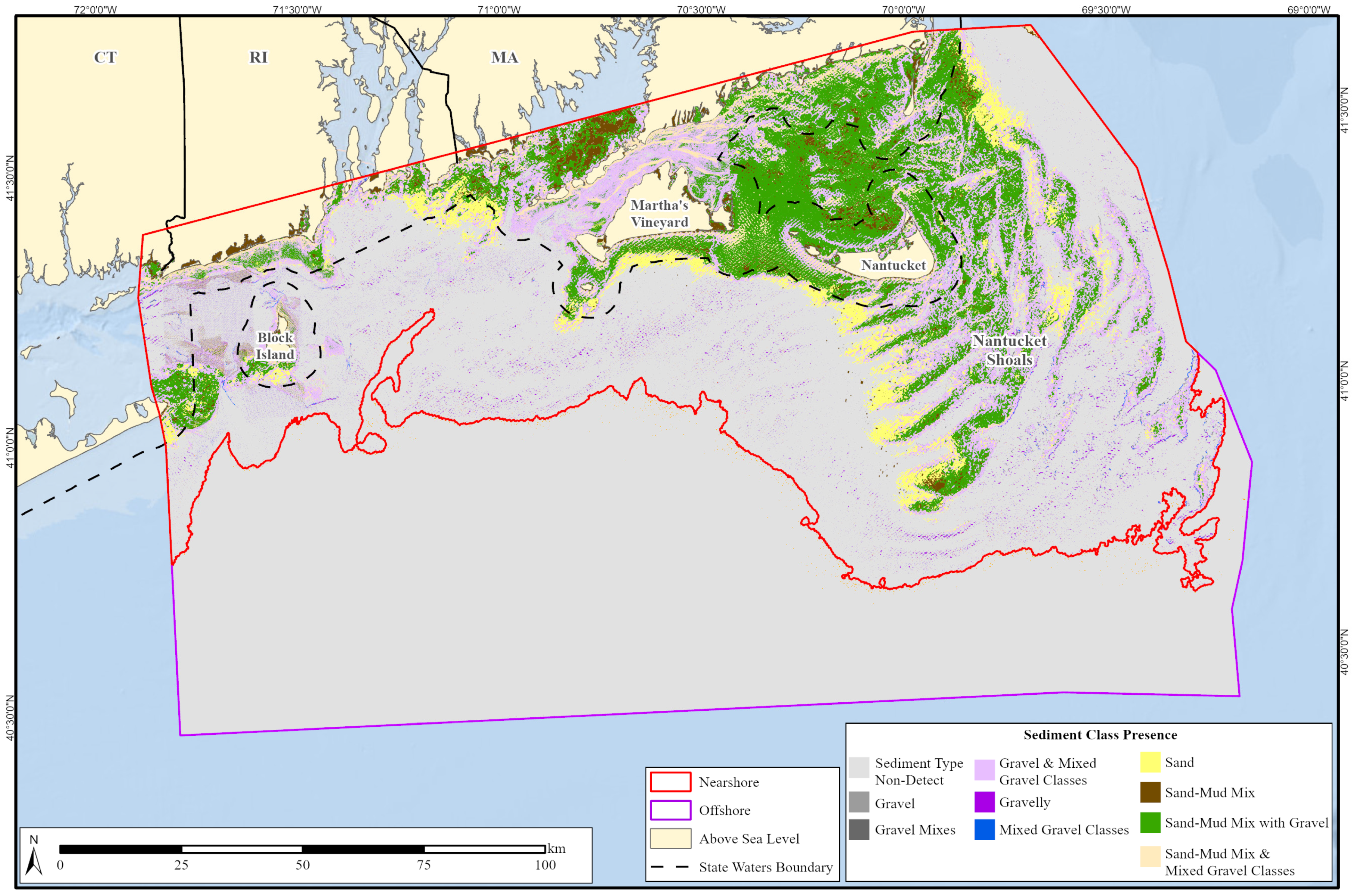
2.3.3. Sediment Composite

To visualize the presence of multiple sediment class model predictions in a single composite image, thresholds were first calculated for each of the five modeled sediment classes using Cohen’s kappa maximum to classify sediment likelihoods as either present or absent. For example, sediment presence likelihoods were converted to a value of 0 (i.e., absent) if less than the calculated threshold or a value or 1 (i.e., present) if above said threshold. However, in the study area’s offshore region, sediment class presence was sparsely predicted (i.e., low sediment class likelihood) due to the disparity in bathymetric features and sediment sampling compared to nearshore areas. Therefore, to improve the prediction of sediment class presence offshore, thresholds were estimated for each sediment class in areas less (i.e., nearshore) and greater (i.e., offshore) than 45 m in depth (Table 3). In other words, two thresholds were calculated for each sediment class based on area, resulting in a total of ten thresholds. When a threshold was calculated below 0.5, a default threshold of 0.5 was used to conservatively estimate the presence of sediment classes.
Presence–absence distributions for each sediment class were then merged and summarized to properly characterize benthic habitat complexity for each grid cell. To achieve this, presence values for each sediment class were reclassified as unique non-zero values (e.g., Gravel = 1, Gravel Mixes = 2, etc.). By stacking reclassified sediment class distributions and summing unique non-zero presence values, a sediment composite was generated where each grid cell contained mutually exclusive scores and thus sediment class combinations. The sediment composite was qualitatively compared between regions with high and low bathymetric sources as well as against publicly available regional sediment data products to gauge composite accuracy and performance.

3. Results

3.1. Sediment Class Predictions

Overall, the generated sediment composite indicated high confidence in sediment occurrence for coastal areas, especially for bathymetric relief associated with Nantucket Shoals, and low predictive confidence in offshore areas (Figure 4). Given the overlay protocol applied to the MaxEnt modeling outputs for the original five sediment classes, nine unique sediment class combinations were used to characterize surficial sediment distributions (Table 4; Figure 4). Sand–Mud Mix with Gravel (10.1%) and Gravel and Mixed Gravel Classes (8.7%) were the most prominent sediment class combinations predicted to occur in the study area. When examining the nearshore and offshore regions, the Sand–Mud Mix with Gravel (17.4%) and Gravel and Mixed Gravel classes (14.9%) were still the most common classes in the nearshore region as compared to Gravelly (0.2%) and Sand–Mud Mix (0.1%) in the offshore region.
Due to the paucity of data, the model successfully characterized sediment in only 27.9% (884.3 km2) of the entire study area. Sediment classes in the remaining 72.1% (2284.73 km2) of the study area could not be characterized given the low confidence in sediment predictions. When separated by region, the model confidently characterized a larger percentage of the nearshore area (48.8%) as compared to the offshore region (~0.2%) (Table 4; Figure 4).

3.2. Model Performance

The bathymetric explanatory variables of depth (80.5%) and geodesic slope (16.5%) were deemed most important, on average, when predicting sediment class occurrence (Table 5). Variable responses curves indicated that, in general, sediment occurrence predictions decreased with increasing depths except for Gravelly, which had an increase in prediction at approximately 40 m. With respect to geodesic slope, occurrence predictions for most sediment classes increased at seafloor slopes greater than 0 degrees (i.e., no seafloor gradient); Gravelly was more likely to occur at moderate seafloor slopes (0 to 40 degrees) before decreasing. AUC values for all sediment classes ranged from 0.74 (Gravelly) to 0.85 (Gravel) (Table 6), which are considered acceptable in terms of model predictive capability. The average true positive rate across all sediment classes, 0.71, was higher than the average true negative rate of 0.59, indicating that the models overall were better at positive detections of sediment classes. The multi-class weighted F1 score, which accounts for class imbalance, was estimated at 0.7. Model prediction uncertainty in occurrence data ranged from 0 to 0.6 (standard deviation) across the study area for all sediment classes with greater uncertainty occurring in the coastal areas of the nearshore region.

4. Discussion

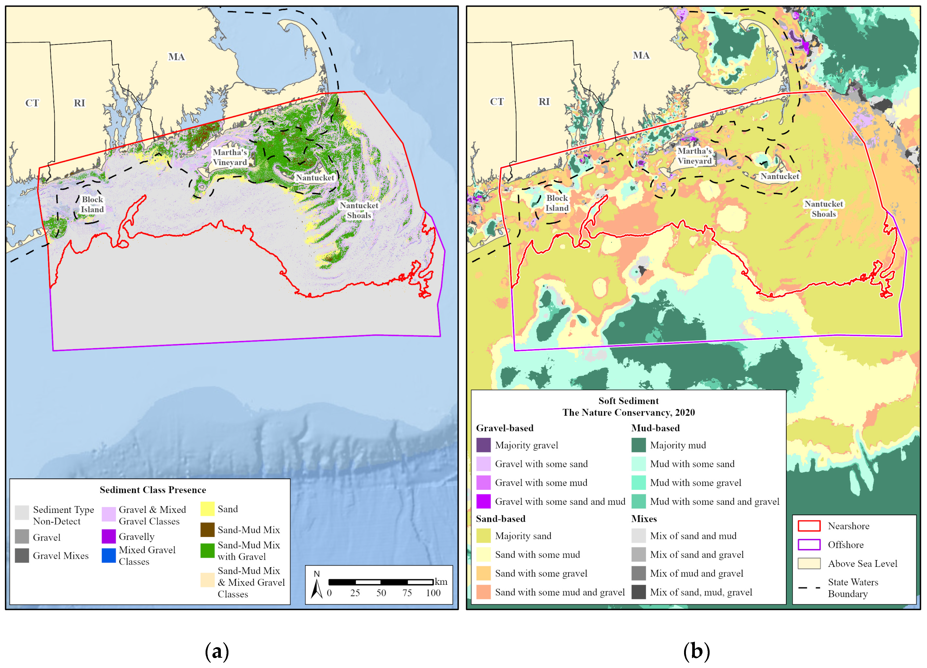
4.1. Assessment of Sediment Composite

In general, the generated sediment composite effectively predicted the occurrence of various surficial sediments in the nearshore areas of southern New England where the survey density and resulting data were the greatest. Combinations of Sand–Mud Mix were the most prevalent in the study area and predicted in several areas, including in and around Buzzards Bay and Nantucket Sound and shallow portions of Nantucket Shoals south of Massachusetts, and often bordered by Sand. Gravel and Mixed Gravel classes were also predicted in nearshore areas, mainly in Vineyard Sound and off the southern coast of mainland Rhode Island and Block Island. Yet, due to the paucity and quality of publicly available data in the region, the current workflow could not confidently predict and classify sediment distributions over most of the study area (~70%). Individual sediment occurrence models were reasonably effective in distinguishing sediment presence, but overall accuracy and uncertainty estimates suggest there is room for improvement.
Nevertheless, the provided workflow and generated sediment composite contribute to the expanding body of research on benthic habitat mapping, especially existing efforts off northeastern US. Predicted distributions in the current sediment composite, for instance, generally agree with seafloor characterizations described for nearshore areas of Massachusetts (e.g., Buzzards Bay, Vineyard Sound, and the southern margin of Martha’s Vineyard) [56], Nantucket Shoals [37], and the northern margin of Block Island [57]. Yet, due to the applied methodology and available bathymetric data, the sediment composite’s fine-scale patterning identifies complex patterns of habitat composition and distribution over a large spatial extent that are not identified by other studies and regional data products. This is particularly true for the Northwest Atlantic Marine Ecoregional Assessment (NAMERA) interpolated soft sediment data product updated in 2020 [58], which does not accurately depict the large and distinct bathymetric relief and sandy composition of the Nantucket Shoals area (Figure 5 and Figure 6). However, the NAMERA data product is based on interpolated grain size data and does not set thresholds for data inclusion, allowing it to yield grain size estimates for offshore areas where sediment occurrences could not be confidently predicted in the current sediment composite. Therefore, given its observed strengths and limitations, the sediment composite is intended to complement other surficial sediment data products and should be used in conjunction with them for drawing conclusions.

4.2. Review of Systematic Workflow

The use of an objective and systematic workflow was essential for utilizing public geospatial data and proactively mapping surficial sediment distributions, especially when schedule and financial resources are constrained. The use of CMECS, for instance, increased the size of machine learning datasets as it was able to standardize sediment observations from multiple projects with varying objectives and reporting styles. Spatial processing tools similarly generated a regional-scale environmental dataset from disjointed bathymetric data products that reconciled data quality and computational performance challenges. The results presented herein also show that combining bathymetric data with sediment observations using machine learning produces accurate surficial sediment maps more efficiently and with less supervision than manual analysis methods. Finally, instead of interpreting the occurrence likelihood for individual sediment classes, robust statistical thresholds and raster calculations were utilized to produce a comprehensive sediment composite to facilitate easier interpretation.
However, there were several limitations that could have potentially influenced the generation and interpretation of the sediment composite. Given that these challenges are mentioned in greater detail by other studies, e.g., [19,30,59,60,61], the following discussion is not meant to be an exhaustive review but only to demonstrate potential impacts on the outlined workflow and interpretation of the final data product.

4.2.1. Sediment Observations

The paucity and quality of publicly available sediment observations in the region presented a major challenge to confidently predicting and classifying sediments based on model accuracy and uncertainty estimates. Similar modeling efforts by Poti et al. [30] noted several potential hurdles when using sediment observations from public repositories. For instance, the uneven distribution of survey density in the study area could impact model accuracy by failing to capture finer scale patterns in sediment distributions for offshore areas where sampling effort was low. Laboratory-based analyses used to generate the comprehensive USGS usSEABED database may omit hard components like shell and gravel and potentially skew results towards finer particles [18]. Additional challenges stem from the inclusion of sediment observations over multiple decades (Supplementary Figure S1), which introduces temporal variation in grain size and sediment composition information. Samples gathered in earlier years may therefore not accurately portray current seafloor conditions, potentially affecting model accuracy, which can be further exacerbated by increased positional uncertainty for older survey data [30,62].
The lack of true absence records in the study area also poses a significant obstacle to accurately predicting sediment distributions. In the present study, for instance, MaxEnt models were informed on the occurrence of specific sediment classes using presence-only data. These models demonstrated higher sensitivity than specificity, indicating they were more adept in correctly identifying instances where sediments were present as compared to the absence of said sediments. While presence record patterns are influenced by various factors that impact absences, the actual distribution of a species or habitat cannot be estimated without data on its absence from suitable areas [63,64]. The collection of true absence records, however, is a resource-intense and complex process, especially considering the inherent biases of characterizing sediments when using various sampling techniques [20]. For instance, sediment grabs offer direct access to sediment samples for estimating grain size but often exhibit biases towards capturing more fine sediments. Although underwater imagery techniques like sediment profile imaging and plan view imaging can capture high-resolution images of undisturbed sediment conditions, characterization requires additional laboratory analysis that can be impacted by overall visibility, angle of observation, and ability to discern small sediment structures. Consequently, a comprehensive set of sampling techniques is therefore necessary to reliably identify absence records and support the development of accurate sediment distribution models.

4.2.2. Environmental Data

Publicly available bathymetric data were vital to the proposed workflow, providing essential environmental information for prediction sediment distributions across the study, but posed their own analytical challenges. For instance, similar to sediment observations, current bathymetric data products in the region were generated from historical survey efforts that could mispresent current seafloor morphological characteristics and impact model accuracy. Spatial scale is another important consideration when collecting acoustic remote sensing data as derived resolutions are often not appropriate for detecting or representing important topographic features [65]. High-resolution bathymetric data (2 m to 8 m) were available for only a portion of the study area, while the rest was comprised by lower-resolution data (250 m). Low-resolution data in the present study, while more detailed than global data products [35], could not capture the fine-scale environmental characteristics necessary for characterizing sediment distributions, e.g., models relying solely on such low-resolution bathymetric data in areas with minor slope changes fail to accurately capture and predict the diversity of benthic habitats. Such differences are evident in the generated sediment composite where more natural sediment distribution patterns were predicted in Vineyard and Nantucket Sound (10 m resolution) as compared to coarser characterizations in areas south of Martha’s Vineyard (250 m resolution) (Figure 7). Future seafloor mapping efforts should use a multi-scale approach, or one that considers data at multiple successive scales, to ensure that scale-dependent benthic processes and distributions are fully captured [61].
Although vital for providing environmental predictor information throughout the study area, the use of bathymetric data for surficial sediment mapping is not a substitute for other acoustic remote sensing data. Indeed, bathymetric data and derived terrain variables (e.g., slope, orientation, curvature) have provided the basis for numerous benthic habitat mapping initiatives, e.g., [25,33,52,66,67]. However, these variables only provide information on seafloor morphology and are indirectly used to identify substrates, e.g., local relief is used as a substitute since rocky areas typically exhibit high local relief [24]. Acoustic backscatter data, in contrast, can provide information regarding the seafloor’s physical properties and composition that can support the characterization of benthic sediments [22,26]. The combination of high-resolution bathymetric data and calibrated backscatter information has enhanced the accuracy and interpretation of surficial sediment maps, e.g., [24,31,32,62,68,69,70]. Yet, despite the demonstrated performance using both types of data, the acquisition, processing, and interpretation of backscatter data are difficult, impacting the integration of results from different mapping systems and regional efforts [60].

4.2.3. MaxEnt Modeling

MaxEnt modeling was critical to successfully predicting the occurrence likelihood of specific sediment classes due to the accessibility of presence-only sediment data. However, MaxEnt modeling assumes that presence-only data were sampled in either a systematic or random fashion over the entire area [59]. In practice, presence-only data are often collected unevenly across an area where survey effort is strongly biased towards more accessible or better-surveyed areas [59,71]. Such spatial bias can severely impact model quality and predictive accuracy as it can incorrectly emphasize the significance of some environmental predictors and under-report the significance of others [59,72]. Publicly available sediment observations in the present study were distributed unevenly in the study area where survey effort was over-represented in nearshore areas. Because survey effort distribution was unavailable, such bias was not corrected for and could have influenced overall model accuracy.
One potential solution to addressing survey bias is the use of presence–absence modeling approaches. Presence–absence data, in contrast to presence-only, are less susceptible to issues associated with survey bias as they provide information on where a species or habitat is present and absent, thereby allowing models to better account for the true environmental parameters and delineate suitable areas [59,72]. Although the use of pseudo-absences, or locations where a species or habitat is assumed to be absent based on available information, have become increasingly common to address survey bias, e.g., [59], these are not true absence records and do not fully mitigate bias in model training, as reviewed in [72]. As such, it is generally advisable to use presence–absence modeling methods when said data are available to reduce these biases and capitalize on all available data for accurately mapping distributions [50]. Although presence–absence data were not publicly available for use in the present study, the explanatory value provided by said data highlights the importance of more comprehensive sediment sampling efforts in the future.

4.3. Recommendations and Future Directions

Based on the limitations presented herein and their impact on mapping products generated, access to a larger collection of publicly available seafloor data is essential to support proactive investigations. Indeed, this in itself poses a significant challenge for many entities that are conducting seafloor data collection activities due to the effort and resources required to cover sufficient temporal and spatial scales. Yet, while these factors limit data collection by government agencies and academic institutions, offshore wind energy developers collect seafloor data to fulfill permitting requirements and, at later intervals, to inform engineering and construction design decisions. These site characterization activities collect sediment and acoustic remote sensing data in offshore wind project areas and transmission cable corridors, often yielding observations and environmental data that better represent true seafloor conditions compared to historical information. Furthermore, this suite of developer acoustic remote sensing data, including bathymetry, backscatter, and side-scan sonar, is collected at resolutions finer than many of the publicly available datasets used in the present study (e.g., <1 m), which can improve the predictive accuracy of modeling approaches and detect fine-scale habitat changes.
Nevertheless, while government agencies provide general guidance and recommendations to wind developers regarding the collection of these seafloor data [73,74,75], no standard protocols exist for collecting, sharing, or reporting these data. As a result, offshore wind developers lack a consistent approach to field data collection, processing, and analysis, leading to variations in spatial coverage, applied methods, and sampled parameters. A review of publicly available Construction and Operations Plans, for instance, found that seafloor acoustic remote sensing, imagery, and grab methods are often not used consistently, and the footprints of data collection activities vary dramatically within and around projects areas [76]. Acoustic remote sensing data were typically unavailable for public inspection due to containing propriety information, while sediment observations were provided in a variety of parameters and file formats that hinder integration efforts.
With the rapid expansion of the offshore wind industry in the US, there is a paramount need for the consistent collection of seafloor data across studies to inform the responsible and cost-effective development of offshore wind energy. Therefore, to ensure regional coordination and address developer concerns, future discussions on seafloor data collection activities should include not only offshore wind developers but also other regional entities. Collaborative forums like the Regional Wildlife Science Collaborative for Offshore Wind (RWSC) are already well positioned to facilitate communication between these stakeholder groups to identify and coordinate seafloor data needs, establish data collection standards, and explore secure data sharing agreements that address confidentiality concerns between stakeholders. Adherence to these community recommendations will dramatically enhance the transfer and integration of multiple collection efforts to aid in the development and maintenance of regional data products. Such efforts will ultimately benefit offshore wind energy developer and stakeholder activities, such as improving the accuracy and detail of environmental assessments, expediting the permitting process, and supporting long-term planning and monitoring decisions.

5. Conclusions

Overall, the present study illustrates the value of using a systematic workflow to integrate public geospatial data and generate regional-scale surficial sediment maps when field data collection activities are not feasible. The approach was capable of transforming a limited set of independently collected sediment observations and acoustic remote sensing data into an ecologically meaningful data product for use by multiple stakeholders. However, despite using national classification standards, spatial processing tools, and machine learning models, the availability and quality of public geospatial data presented several challenges for accurately predicting and characterizing surficial sediments throughout the designated study area. Although the supposition that ongoing seafloor data collection efforts will bolster these public repositories, the lack of defined data collection standards and data sharing agreements may only maintain the status quo when synthesizing regional products. As such, regional coordination with existing and ongoing seafloor mapping efforts is crucial to the standard collection and delivery of environmental data that will ultimately support ecologically responsible offshore wind energy decisions.

Supplementary Materials

The following supporting information can be downloaded at: https://www.mdpi.com/article/10.3390/geosciences14070186/s1, Table S1: Publicly available sediment and bathymetric datasets used to predict and characterize sediment class occurrence in the study area. Datasets are organized by type, specifically sediment observations and bathymetric data products, and accompanied by various metadata, including dataset title, source, date published, survey dates for collecting data, applied sampling technique, file format, and online hyperlink for access; Table S2: Number of sediment records collected during the desktop data review and applied to the machine learning approach for each sediment class. Machine learning values identify the number of observations used to train and test the maximum entropy models developed for each sediment class; Figure S1: Time series of sediment observations identified during the desktop data review and the year they were originally collected. Sediment records were primarily collected between 1930 and 2020 but date back as early as 1842; Figure S2: Sediment class presence predictions for Gravel Mixes using terrain variables from bathymetric data products with resolutions of 4 m (left) and 8 m (right). The systematic workflow presented herein was applied to a small case study in the northwestern Atlantic Ocean, specifically in the coastal waters of Massachusetts (MA) in the western Gulf of Maine. The comparison is meant to demonstrate the negligible difference in sediment presence patterning when high-resolution data are down-sampled to resolutions that are more equitable for intense computational processing.

Author Contributions

Conceptualization, E.J.S. and M.L.G.; methodology, A.C.R., B.G.T., C.W.C. and M.L.G.; software, A.C.R., B.G.T. and J.A.C.; data curation, processing, and visualization, B.G.T. and J.A.C.; formal analysis, A.C.R.; data review and interpretation, C.W.C. and M.L.G.; writing—original draft preparation, C.W.C.; writing—review and editing, C.W.C., E.J.S. and M.L.G.; supervision and project administration, C.W.C. and M.L.G.; funding acquisition, E.J.S. and M.L.G. All authors have read and agreed to the published version of the manuscript.

Funding

This research was funded by the Massachusetts Clean Energy Technology Center (GG-2002-16277).

Data Availability Statement

Sediment observations and bathymetric data used in modeling approach are accessible to the public (see Supplementary Table S1 for details). Further inquiries can be directed at the corresponding authors.

Acknowledgments

The authors would like to thank the Seafloor Habitat Data Work Group for providing input and recommending both data sources and methods for the present study; the Habitat & Ecosystem Subcommittee of the Regional Wildlife Science Collaborative for Offshore Wind (RWSC) for providing feedback on the system workflow and sediment composite; M. Poti (NOAA National Centers for Coastal Ocean Sciences) for providing input on the statistical analysis and sediment composite generation.

Conflicts of Interest

Author Connor W. Capizzano, Alexandria C. Rhoads, Jennifer A. Croteau, Benjamin G. Taylor and Marisa L. Guarinello were employed by the INSPIRE Environmental Inc. The remaining author declare that the research was conducted in the absence of any commercial or financial relationships that could be construed as a potential conflict of interest.

References

  1. Owusu, P.A.; Asumadu-Sarkodie, S. A Review of Renewable Energy Sources, Sustainability Issues and Climate Change Mitigation. Cogent Eng. 2016, 3, 1167990. [Google Scholar] [CrossRef]
  2. Olabi, A.G.; Abdelkareem, M.A. Renewable Energy and Climate Change. Renew. Sustain. Energy Rev. 2022, 158, 112111. [Google Scholar] [CrossRef]
  3. The White House. FACT SHEET: Biden-Harris Administration Continues to Advance American Offshore Wind Opportunities. The White House. 2023. Available online: https://www.whitehouse.gov/briefing-room/statements-releases/2023/03/29/fact-sheet-biden-harris-administration-continues-to-advance-american-offshore-wind-opportunities/ (accessed on 31 May 2024).
  4. Global Wind Energy Council. Global Offshore Wind Report 2023. Available online: https://gwec.net/gwecs-global-offshore-wind-report-2023/ (accessed on 31 May 2024).
  5. Musial, W.; Spitsen, P.; Duffy, P.; Beiter, P.; Shields, M.; Hernando, D.M.; Hammond, R.; Marquis, M.; King, J.; Sriharan, S. Offshore Wind Market Report: 2023 Edition; U.S. Department of Energy: Washington, DC, USA, 2023.
  6. Methratta, E.T.; Silva, A.; Lipsky, A.; Ford, K.; Christel, D.; Pfeiffer, L. Science Priorities for Offshore Wind and Fisheries Research in the Northeast U.S. Continental Shelf Ecosystem: Perspectives from Scientists at the National Marine Fisheries Service. Mar. Coast. Fish. 2023, 15, e10242. [Google Scholar] [CrossRef]
  7. Galparsoro, I.; Menchaca, I.; Garmendia, J.M.; Borja, Á.; Maldonado, A.D.; Iglesias, G.; Bald, J. Reviewing the Ecological Impacts of Offshore Wind Farms. NPJ Ocean Sustain. 2022, 1, 1. [Google Scholar] [CrossRef]
  8. Methratta, E.; Hawkins, A.; Hooker, B.; Lipsky, A.; Hare, J. Offshore Wind Development in the Northeast US Shelf Large Marine Ecosystem: Ecological, Human, and Fishery Management Dimensions. Oceanography 2020, 33, 16–27. [Google Scholar] [CrossRef]
  9. Harris, P.; Baker, E. (Eds.) Seafloor Geomorphology as Benthic Habitat: GeoHab Atlas of Seafloor Geomorphic Features and Benthic Habitats; Elsevier: Amsterdam, The Netherlands, 2011. [Google Scholar]
  10. Costanza, R.; D’Arge, R.; de Groot, R.; Farber, S.; Grasso, M.; Hannon, B.; Limburg, K.; Naeem, S.; O’Neill, R.V.; Paruelo, J.; et al. The Value of the World’s Ecosystem Services and Natural Capital. Nature 1997, 387, 253–260. [Google Scholar] [CrossRef]
  11. Lefcheck, J.S.; Hughes, B.B.; Johnson, A.J.; Pfirrmann, B.W.; Rasher, D.B.; Smyth, A.R.; Williams, B.L.; Beck, M.W.; Orth, R.J. Are Coastal Habitats Important Nurseries? A Meta-Analysis. Conserv. Lett. 2019, 12, e12645. [Google Scholar] [CrossRef]
  12. Crespo, D.; Pardal, M.Â. Ecological and Economic Importance of Benthic Communities. In Life Below Water; Leal Filho, W., Azul, A.M., Brandli, L., Lange Salvia, A., Wall, T., Eds.; Springer International Publishing: Cham, Switzerland, 2020; pp. 1–11. [Google Scholar]
  13. Airoldi, L.; Balata, D.; Beck, M.W. The Gray Zone: Relationships between Habitat Loss and Marine Diversity and Their Applications in Conservation. J. Exp. Mar. Biol. Ecol. 2008, 366, 8–15. [Google Scholar] [CrossRef]
  14. Kritzer, J.P.; DeLucia, M.-B.; Greene, E.; Shumway, C.; Topolski, M.F.; Thomas-Blate, J.; Chiarella, L.A.; Davy, K.B.; Smith, K. The Importance of Benthic Habitats for Coastal Fisheries. Bioscience 2016, 66, 274–284. [Google Scholar] [CrossRef]
  15. McCauley, D.J.; Pinsky, M.L.; Palumbi, S.R.; Estes, J.A.; Joyce, F.H.; Warner, R.R. Marine Defaunation: Animal Loss in the Global Ocean. Science 2015, 347, 1255641. [Google Scholar] [CrossRef]
  16. Degraer, S.; Carey, D.; Coolen, J.; Hutchison, Z.; Kerckhof, F.; Rumes, B.; Vanaverbeke, J. Offshore Wind Farm Artificial Reefs Affect Ecosystem Structure and Functioning: A Synthesis. Oceanography 2020, 33, 48–57. [Google Scholar] [CrossRef]
  17. Hutchison, Z.; Bartley, M.; Degraer, S.; English, P.; Khan, A.; Livermore, J.; Rumes, B.; King, J. Offshore Wind Energy and Benthic Habitat Changes: Lessons from Block Island Wind Farm. Oceanography 2020, 33, 58–69. [Google Scholar] [CrossRef]
  18. Goff, J.A.; Jenkins, C.J.; Jeffress Williams, S. Seabed Mapping and Characterization of Sediment Variability Using the usSEABED Data Base. Cont. Shelf Res. 2008, 28, 614–633. [Google Scholar] [CrossRef]
  19. Misiuk, B.; Brown, C.J. Benthic Habitat Mapping: A Review of Three Decades of Mapping Biological Patterns on the Seafloor. Estuar. Coast. Shelf Sci. 2024, 296, 108599. [Google Scholar] [CrossRef]
  20. Tuit, C.B.; Wait, A.D. A Review of Marine Sediment Sampling Methods. Environ. Forensics 2020, 21, 291–309. [Google Scholar] [CrossRef]
  21. Mayer, L.A. Frontiers in Seafloor Mapping and Visualization. Mar. Geophys. Res. 2006, 27, 7–17. [Google Scholar] [CrossRef]
  22. Brown, C.J.; Smith, S.J.; Lawton, P.; Anderson, J.T. Benthic Habitat Mapping: A Review of Progress towards Improved Understanding of the Spatial Ecology of the Seafloor Using Acoustic Techniques. Estuar. Coast. Shelf Sci. 2011, 92, 502–520. [Google Scholar] [CrossRef]
  23. Khomsin, M.; Pratomo, D.G.; Suntoyo. The Development of Seabed Sediment Mapping Methods: The Opportunity Application in the Coastal Waters. IOP Conf. Ser. Earth Environ. Sci. 2021, 731, 012039. [Google Scholar] [CrossRef]
  24. Dartnell, P.; Gardner, J.V. Predicting Seafloor Facies from Multibeam Bathymetry and Backscatter Data. Photogramm. Eng. Remote Sens. 2004, 70, 1081–1091. [Google Scholar] [CrossRef]
  25. Elvenes, S.; Dolan, M.F.J.; Buhl-Mortensen, P.; Bellec, V.K. An Evaluation of Compiled Single-Beam Bathymetry Data as a Basis for Regional Sediment and Biotope Mapping. ICES J. Mar. Sci. 2014, 71, 867–881. [Google Scholar] [CrossRef]
  26. Lamarche, G.; Lurton, X. Recommendations for Improved and Coherent Acquisition and Processing of Backscatter Data from Seafloor-Mapping Sonars. Mar. Geophys. Res. 2018, 39, 5–22. [Google Scholar] [CrossRef]
  27. Misiuk, B.; Diesing, M.; Aitken, A.; Brown, C.J.; Edinger, E.N.; Bell, T. A Spatially Explicit Comparison of Quantitative and Categorical Modelling Approaches for Mapping Seabed Sediments Using Random Forest. Geosciences 2019, 9, 254. [Google Scholar] [CrossRef]
  28. Nimon, K.F. Statistical Assumptions of Substantive Analyses Across the General Linear Model: A Mini-Review. Front. Psychol. 2012, 3, 322. [Google Scholar] [CrossRef] [PubMed]
  29. Olden, J.D.; Lawler, J.J.; Poff, N.L. Machine Learning Methods Without Tears: A Primer for Ecologists. Q. Rev. Biol. 2008, 83, 171–193. [Google Scholar] [CrossRef] [PubMed]
  30. Poti, M.; Kinlan, B.; Menza, C. Chapter 3: Surficial Sediments. In A Biogeographic Assessment of Seabirds, Deep Sea Corals and Ocean Habitats of the New York Bight: Science to Support Offshore Spatial Planning; Menza, C., Kinlan, B., Dorfman, D., Poti, M., Eds.; NOAA Technical Memorandum NOS NCCOS 141; NOAA/National Centers for Coastal Ocean Science: Silver Spring, MD, USA, 2012; pp. 33–58. [Google Scholar]
  31. Xu, W.; Cheng, H.; Zheng, S.; Hu, H. Predicted Mapping of Seabed Sediments Based on MBES Backscatter and Bathymetric Data: A Case Study in Joseph Bonaparte Gulf, Australia, Using Random Forest Decision Tree. J. Mar. Sci. Eng. 2021, 9, 947. [Google Scholar] [CrossRef]
  32. Pillay, T.; Cawthra, H.C.; Lombard, A.T.; Sink, K. Benthic Habitat Mapping from a Machine Learning Perspective on the Cape St Francis Inner Shelf, Eastern Cape, South Africa. Mar. Geol. 2021, 440, 106595. [Google Scholar] [CrossRef]
  33. Sklar, E.; Bushuev, E.; Misiuk, B.; Labbé-Morissette, G.; Brown, C.J. Seafloor Morphology and Substrate Mapping in the Gulf of St Lawrence, Canada, Using Machine Learning Approaches. Front. Mar. Sci. 2024, 11, 1306396. [Google Scholar] [CrossRef]
  34. Wölfl, A.-C.; Snaith, H.; Amirebrahimi, S.; Devey, C.W.; Dorschel, B.; Ferrini, V.; Huvenne, V.A.I.; Jakobsson, M.; Jencks, J.; Johnston, G.; et al. Seafloor Mapping—The Challenge of a Truly Global Ocean Bathymetry. Front. Mar. Sci. 2019, 6, 283. [Google Scholar] [CrossRef]
  35. Mayer, L.; Jakobsson, M.; Allen, G.; Dorschel, B.; Falconer, R.; Ferrini, V.; Lamarche, G.; Snaith, H.; Weatherall, P. The Nippon Foundation—GEBCO Seabed 2030 Project: The Quest to See the World’s Oceans Completely Mapped by 2030. Geosciences 2018, 8, 63. [Google Scholar] [CrossRef]
  36. Jackson, S.J.; Barbrow, S. Standards and/as Innovation: Protocols, Creativity, and Interactive Systems Development in Ecology. In Proceedings of the 33rd Annual ACM Conference on Human Factors in Computing Systems, Seoul, Republic of Korea, 18–23 April 2015; ACM: New York, NY, USA, 2015; pp. 1769–1778. [Google Scholar]
  37. Stevenson, D.; Chiarella, L.; Stephen, D.; Reid, R.; Wilhelm, K.; McCarthy, J.; Pentony, M. Characterization of the Fishing Practices and Marine Benthic Ecosystems of the Northeast U.S. Shelf, and an Evaluation of the Potential Effects of Fishing on Essential Fish Habitat; NOAA Technical Memorandum NMFS-NE-181; NOAA/National Centers for Coastal Ocean Science: Silver Spring, MD, USA, 2004.
  38. Wahle, R.; Steneck, R. Recruitment Habitats and Nursery Grounds of the American Lobster Homarus Americanus: A Demographic Bottleneck? Mar. Ecol. Prog. Ser. 1991, 69, 231–243. [Google Scholar] [CrossRef]
  39. Griswold, C.A.; Prezioso, J. In Situ Observations on Reproductive Behavior of the Long-Finned Squid, Loligo Pealei. Fish. Bull. 1981, 78, 945–947. [Google Scholar]
  40. Roper, C.F.E.; Sweeney, M.J.; Nauen, C.E. FAO Species Catalogue: Vol. 3. Cephalopods of the World. An Annotated and Illustrated Catalogue of Species of Interest to Fisheries; FAO Fisheries Synopsis No. 125; FAO: Rome, Italy, 1984; Volume 3. [Google Scholar]
  41. Fahay, M.P.; Berrien, P.L.; Johnson, D.L.; Morse, W.W. Essential Fish Habitat Source Document: Atlantic Cod, Gadus Morhua, Life History and Habitat Characteristics; NOAA/National Marine Fisheries Service, Northeast Fisheries Science Center: Woods Hole, MA, USA, 1999.
  42. Ward, L.; Johnson, P.; Bogonko, M.; McAvoy, Z.; Morrison, R. Northeast Bathymetry and Backscatter Compilation: Western Gulf of Maine, Southern New England, and Long Island Sound; Department of Interior, Bureau of Ocean Energy Management, Marine Minerals Division: Sterling, VA, USA, 2021.
  43. Federal Geographic Data Committee (FGDC). Coastal and Marine Ecological Classification Standard; FGDC-STD-018-2012; Federal Geographic Data Committee (FGDC): Reston, VA, USA, 2012.
  44. Wentworth, C. A Scale of Grade and Class Terms for Clastic Sediments. J. Geol. 1922, 30, 377–392. [Google Scholar] [CrossRef]
  45. Walbridge, S.; Slocum, N.; Pobuda, M.; Wright, D. Unified Geomorphological Analysis Workflows with Benthic Terrain Modeler. Geosciences 2018, 8, 94. [Google Scholar] [CrossRef]
  46. R Core Team. R: A Language and Environment for Statistical Computing; R Foundation for Statistical Computing: Vienna, Austria, 2022; Available online: https://www.r-project.org/ (accessed on 30 March 2022).
  47. Hijmans, R.; Phillips, S.; Leathwick, J.; Elith, J. Dismo: Species Distribution Modeling. R Package Version 1.3.5. Available online: https://cran.r-project.org/web/packages/dismo/index.html (accessed on 29 May 2024).
  48. Urbanek, S. RJava: Low-Level R to Java Interface. R Package Version 1.0.6. Available online: https://cran.r-project.org/web/packages/rJava/index.html (accessed on 29 May 2024).
  49. Elith, J.; Graham, C.; Anderson, R.; Dudík, M.; Ferrier, S.; Guisan, A.; Hijmans, R.; Huettmann, F.; Leathwick, J.; Lehmann, A.; et al. Novel Methods Improve Prediction of Species’ Distributions from Occurrence Data. Ecography 2006, 29, 129–151. [Google Scholar] [CrossRef]
  50. Elith, J.; Phillips, S.J.; Hastie, T.; Dudík, M.; Chee, Y.E.; Yates, C.J. A Statistical Explanation of MaxEnt for Ecologists. Divers. Distrib. 2011, 17, 43–57. [Google Scholar] [CrossRef]
  51. Phillips, S.J.; Anderson, R.P.; Schapire, R.E. Maximum Entropy Modeling of Species Geographic Distributions. Ecol. Model. 2006, 190, 231–259. [Google Scholar] [CrossRef]
  52. Howell, K.L.; Holt, R.; Endrino, I.P.; Stewart, H. When the Species Is Also a Habitat: Comparing the Predictively Modelled Distributions of Lophelia Pertusa and the Reef Habitat It Forms. Biol. Conserv. 2011, 144, 2656–2665. [Google Scholar] [CrossRef]
  53. Tittensor, D.; Baco, A.; Brewin, P.; Clark, M.; Consalvey, M.; Hall-Spencer, J.; Rowden, A.; Schlacher, T.; Stocks, K.; Rogers, A. Predicting Global Habitat Suitability for Stony Corals on Seamounts. J. Biogeogr. 2009, 36, 1111–1128. [Google Scholar] [CrossRef]
  54. Melo, F. Area under the ROC Curve. In Encyclopedia of Systems Biology; Springer: New York, NY, USA, 2013; pp. 38–39. [Google Scholar]
  55. Mandrekar, J. Receiver Operating Characteristic Curve in Diagnostic Test Assessment. J. Thorac. Oncol. 2010, 5, 1315–1316. [Google Scholar] [CrossRef]
  56. Massachusetts Office of Coastal Zone Management (MassCZM). Sediment and Geology Workgroup Report; Massachusetts Office of Coastal Zone Management (MassCZM): Boston, MA, USA, 2020.
  57. Poppe, L.J.; Danforth, W.W.; McMullen, K.Y.; Blankenship, M.A.; Glomb, K.A.; Wright, D.B.; Smith, S.M. Sea-Floor Character and Sedimentary Processes of Block Island Sound, Offshore Rhode Island (ver.1.1, August 2014): U.S. Geological Survey Open-File Report 2012–1005. 2012. Available online: http://pubs.usgs.gov/of/2012/1005/ (accessed on 31 May 2024).
  58. Anderson, M.; Green, J.; Morse, D.; Shumway, D.; Clark, M. Benthic Habitats of the Northwest Atlantic. In The Northwest Atlantic Marine Ecoregional Assessment: Species, Habitats and Ecosystems. Phase One; Greene, J., Anderson, M., Odell, J., Steinberg, N., Eds.; The Nature Conservancy, Eastern U.S. Division: Boston, MA, USA, 2010; pp. 3-1–3-61. [Google Scholar]
  59. Phillips, S.J.; Dudík, M.; Elith, J.; Graham, C.H.; Lehmann, A.; Leathwick, J.; Ferrier, S. Sample Selection Bias and Presence-only Distribution Models: Implications for Background and Pseudo-absence Data. Ecol. Appl. 2009, 19, 181–197. [Google Scholar] [CrossRef]
  60. Lurton, X.; Lamarche, G. Backscatter Measurements by Seafloor-Mapping Sonars. Guidelines and Recommendations. 2015. 200p. Available online: https://zenodo.org/records/10089261 (accessed on 30 March 2024).
  61. Lecours, V.; Devillers, R.; Schneider, D.; Lucieer, V.; Brown, C.; Edinger, E. Spatial Scale and Geographic Context in Benthic Habitat Mapping: Review and Future Directions. Mar. Ecol. Prog. Ser. 2015, 535, 259–284. [Google Scholar] [CrossRef]
  62. Diesing, M.; Green, S.L.; Stephens, D.; Lark, R.M.; Stewart, H.A.; Dove, D. Mapping Seabed Sediments: Comparison of Manual, Geostatistical, Object-Based Image Analysis and Machine Learning Approaches. Cont. Shelf Res. 2014, 84, 107–119. [Google Scholar] [CrossRef]
  63. Lobo, J.M. More Complex Distribution Models or More Representative Data? Biodivers. Inform. 2008, 5, 14–19. [Google Scholar] [CrossRef]
  64. Jiménez-Valverde, A.; Lobo, J.M.; Hortal, J. Not as Good as They Seem: The Importance of Concepts in Species Distribution Modelling. Divers. Distrib. 2008, 14, 885–890. [Google Scholar] [CrossRef]
  65. Misiuk, B.; Lecours, V.; Bell, T. A Multiscale Approach to Mapping Seabed Sediments. PLoS ONE 2018, 13, e0193647. [Google Scholar] [CrossRef] [PubMed]
  66. Gormley, K.S.G.; Porter, J.S.; Bell, M.C.; Hull, A.D.; Sanderson, W.G. Predictive Habitat Modelling as a Tool to Assess the Change in Distribution and Extent of an OSPAR Priority Habitat under an Increased Ocean Temperature Scenario: Consequences for Marine Protected Area Networks and Management. PLoS ONE 2013, 8, e68263. [Google Scholar] [CrossRef]
  67. Huang, Z.; Brooke, B.P.; Harris, P.T. A New Approach to Mapping Marine Benthic Habitats Using Physical Environmental Data. Cont. Shelf Res. 2011, 31, S4–S16. [Google Scholar] [CrossRef]
  68. Huang, Z.; Siwabessy, J.; Nichol, S.L.; Brooke, B.P. Predictive Mapping of Seabed Substrata Using High-Resolution Multibeam Sonar Data: A Case Study from a Shelf with Complex Geomorphology. Mar. Geol. 2014, 357, 37–52. [Google Scholar] [CrossRef]
  69. Calvert, J.; Strong, J.A.; Service, M.; McGonigle, C.; Quinn, R. An Evaluation of Supervised and Unsupervised Classification Techniques for Marine Benthic Habitat Mapping Using Multibeam Echosounder Data. ICES J. Mar. Sci. 2015, 72, 1498–1513. [Google Scholar] [CrossRef]
  70. Diesing, M.; Mitchell, P.J.; O’Keeffe, E.; Gavazzi, G.O.A.M.; Bas, T. Le Limitations of Predicting Substrate Classes on a Sedimentary Complex but Morphologically Simple Seabed. Remote Sens. 2020, 12, 3398. [Google Scholar] [CrossRef]
  71. Kramer-Schadt, S.; Niedballa, J.; Pilgrim, J.D.; Schröder, B.; Lindenborn, J.; Reinfelder, V.; Stillfried, M.; Heckmann, I.; Scharf, A.K.; Augeri, D.M.; et al. The Importance of Correcting for Sampling Bias in MaxEnt Species Distribution Models. Divers. Distrib. 2013, 19, 1366–1379. [Google Scholar] [CrossRef]
  72. Elith, J.; Graham, C.; Valavi, R.; Abegg, M.; Bruce, C.; Ford, A.; Guisan, A.; Hijmans, R.J.; Huettmann, F.; Lohmann, L.; et al. Presence-Only and Presence-Absence Data for Comparing Species Distribution Modeling Methods. Biodivers. Inform. 2020, 15, 69–80. [Google Scholar] [CrossRef]
  73. Bureau of Ocean Energy Management (BOEM), Office of Renewable Energy Programs. Guidelines for Providing Geophysical, Geotechnical, and Geohazard Information Pursuant to 30 CFR Part 585; BOEM: Washington, DC, USA, 2020.
  74. Bureau of Ocean Energy Management (BOEM), Office of Renewable Energy Programs. Guidelines for Providing Benthic Habitat Survey Information for Renewable Energy Development on the Atlantic Outer Continental Shelf Pursuant to 30 CFR Part 585; BOEM: Washington, DC, USA, 2019.
  75. National Marine Fisheries Service (NOAA Fisheries), Greater Atlantic Regional Fisheries Office, Habitat Conservation and Ecosystem Services Division. Recommendations for Mapping Fish Habitat; NOAA/National Marine Fisheries Service, Greater Atlantic Regional Fisheries Office: Gloucester, MA, USA, 2021.
  76. Regional Wildlife Science Collaborative for Offshore Wind (RWSC). Integrated Science Plan for Offshore Wind, Wildlife, and Habitat in U.S. Atlantic Waters. Version 1.0. Available online: https://rwsc.org/science-plan (accessed on 31 May 2024).
Figure 1. Data collected within the study area off the northeastern United States in the waters south of Connecticut (CT), Rhode Island (RI), and Massachusetts (MA). Bathymetric data are visually depicted using a color gradient in the background, whereas in situ sediment sampling data are shown with black dots in the foreground.
Geosciences 14 00186 g001
Figure 2. Established workflow for generating a sediment composite using publicly available geospatial data and machine learning. The workflow includes (1) the extraction and preparation of explanatory and response variables from collected data, (2) the building and testing of maximum entropy (MaxEnt) machine learning models for each sediment class, and (3) the generation of a sediment composite by converting predicted sediment class likelihoods to presence–absence outputs and overlaying them. The number of predictor variables are indicated within parentheses, whereas the number of categories for the single response variable are shown inside brackets.
Geosciences 14 00186 g002
Figure 3. Correlation plot matrix displaying Pearson correlation coefficient values between variables extracted from the bathymetric mosaic dataset using the Benthic Terrain Modeler extension [45] (see Table 2).
Geosciences 14 00186 g003
Figure 4. Predicted occurrence of nine sediment class combinations within the study area using a systematic workflow. The nearshore–offshore region boundary identifies where different sets of thresholds were used to classify sediment occurrence likelihoods as either present or absent prior to raster calculations. The term “Sediment Type Non-Detect” references areas where sediment classes could not be properly characterized due to low prediction confidence.
Geosciences 14 00186 g004
Figure 5. Regional comparison of (a) the generated sediment composite with (b) the Northwest Atlantic Marine Ecological Assessment interpolated soft sediment data product based on interpolated grain size data.
Geosciences 14 00186 g005
Figure 6. Site-specific comparison of (a) the generated sediment composite with (b) the Northwest Atlantic Marine Ecological Assessment interpolated soft sediment data product based on interpolated grain size data.
Geosciences 14 00186 g006
Figure 7. Comparison of predicated sediment occurrence patterns using bathymetric environmental data of varying resolutions, specifically 10 m resolution in Vineyard Sound and 250 m resolution in the coastal areas south of Martha’s Vineyard.
Geosciences 14 00186 g007
Table 1. Sediment grain size classification descriptors for the Wentworth Scale [44] and the Coastal and Marine Ecological Classification Standard (CMECS) [43].
Wentworth ScaleCMECS 1
Phi Size
(Φ)
Size Range
(mm)
Size ClassSubstrate Group
(Substrate Subgroup) 2
Grain Size
(mm)
Class Sizes
(phi)
Gravel 32 to <4096−1 to <−12
<−8>256Boulder(Boulder)256 to <4096−8 to <−12
−7 to −8128 to 256Cobble(Cobble)64 to <256−6 to <−8
−6 to −764 to 128Cobble
−5 to −632 to 64Very coarse pebble(Pebble)4 to <64−1 to <−6
−4 to −516 to 32Coarse pebble
−3 to −48 to 16Medium pebble
−2 to −34 to 8Fine pebble
−1 to −22 to 4Very fine pebble(Granule)2 to <4−1 to <−2
Sand0.0625 to <24 to <−1
0 to −11 to 2Very coarse sand(Very Coarse Sand)1 to <20 to <−1
1 to 00.5 to 1Coarse sand(Coarse Sand)0.5 to <11 to <0
2 to 10.25 to 0.5Medium sand(Medium Sand)0.25 to <0.52 to <1
3 to 20.125 to 0.25Fine sand(Fine Sand)0.125 to <0.253 to <2
4 to 30.0625 to 0.125Very find sand(Very Fine Sand)0.0625 to <0.1254 to <3
>4<0.0625Silt/clayMud<0.0625>4
(Silt)0.004 to <0.0625>4 to 8
(Clay)<0.004>8
1 CMECS uses the term Mud to describe all particles smaller than sand (less than 0.0625 mm). 2 Values in parentheses represent Subgroups of the overarching Substrate Group (e.g., Boulder is a Subgroup of the Substrate Group Gravel). 3 The term Gravel is used to describe all rock fragment particles that are 2 mm or larger.
Table 2. Explanatory variables extracted from the bathymetric mosaic dataset using Benthic Terrain Modeler [45]. Inner and outer radii were used to calculate bathymetric position indices. Abbreviations serve as a reference for the Pearson correlation coefficient analysis between these nine variables (see Figure 3).
VariablesAbbreviationDefinition
Depth (m) *DepthWater depth in meters
Geodesic Slope *SlopeMeasure of gradient
Aspect—N/S *AspectNGradient in north/south direction
Aspect—E/W *AspectEGradient in east/west direction
Curvature, Profile *Curv-ProfileMeasure of ‘exposure’; parallel direction, benthic flow
Curvature, Planar *Curve-PlanMeasure of ‘exposure’; perpendicular direction, benthic convergence
Bathymetric Position Index, Fine (8, 10)BPI 8–10Measure of relative surrounding elevation, fine (peaks+, depressions−, plateau 0)
Bathymetric Position Index, Broad (8, 25) *BPI 8–25Measure of relative surrounding elevation, broad (peaks+, depressions−, plateau 0)
Bathymetric Position Index, Broad (8, 75)BPI 8–75Measure of relative surrounding elevation, broad (peaks+, depressions−, plateau 0)
* Variable was retained in the final maximum entropy (MaxEnt) model.
Table 3. Estimated threshold values for converting the predicted likelihood of each sediment class occurring within each nearshore and offshore location into a binary presence–absence output.
Region
Sediment ClassNearshoreOffshore
Gravel0.46 *0.49 *
Gravel Mixes0.740.67
Gravelly0.810.71
Sand0.45 *0.40 *
Sand–Mud Mix0.39 *0.76
* In instances where estimated thresholds were low, a default value of 0.50 was used to conservatively estimate sediment occurrence.
Table 4. Estimated area occurrence of nine sediment class combinations within the study area. Area of occurrence estimates are provided in square kilometers [km2] and percent (%) by sediment class combination for the entire study as well as nearshore and offshore portions.
OverallNearshoreOffshore
Sediment ClassArea (km2)Area (%)Area (km2)Area (%)Area (km2)Area (%)
Gravel6.670.216.670.3600
Gravel Mixes3.160.103.140.170.020
Gravel and Mixed Gravel Classes274.178.65274.1514.870.010
Gravelly54.491.7252.252.832.240.17
Mixed Gravel Classes4.580.144.550.250.030
Sand94.222.9794.225.1100
Sand–Mud Mix57.011.8056.323.050.690.05
Sand–Mud Mix with Gravel320.8510.12320.8517.4000
Sand–Mud Mix and Mixed Gravel Classes69.142.1868.973.740.170.01
Not Classified2284.7372.10962.3852.201322.3499.76
Table 5. Variable importance of bathymetric variables for predicting sediment occurrence in terms of percent contribution. A mean percent contribution identifies the average contribution of each variable across sediment classes.
Percent Contribution
VariableGravel MixesGravelGravellySandSand–Mud MixMean
Depth (m)68.267.977.994.49480.48
Geodesic Slope28.831.811.85.2516.52
Aspect—N/S1.20.280.30.62.06
Aspect—E/W1.30.11.90.10.10.70
Curvature, Profile000000.00
Curvature, Planar0.400000.08
Bathymetric Position Index (8, 25)000.300.30.12
Table 6. Model performance metrics derived from sediment class-specific confusion matrices, including the area under curve (AUC) value from the receiver-operating characteristic curves, accuracy, sensitivity (true positive rate), specificity (true negative rate), and F1 score.
Metrics
Sediment ClassAUCAccuracySensitivitySpecificityF1
Gravel0.850.660.730.630.61
Gravel Mixes0.820.590.770.560.40
Gravelly0.740.550.720.530.28
Sand0.820.650.660.640.73
Sand–Mud Mix0.770.640.660.600.72
Disclaimer/Publisher’s Note: The statements, opinions and data contained in all publications are solely those of the individual author(s) and contributor(s) and not of MDPI and/or the editor(s). MDPI and/or the editor(s) disclaim responsibility for any injury to people or property resulting from any ideas, methods, instructions or products referred to in the content.

