

Cenozoic Carbon Dioxide: The 66 Ma Solution


SLAC National Accelerator Laboratory, Stanford University, Menlo Park, CA 94025, USA
Geosciences 2024, 14(9), 238; https://doi.org/10.3390/geosciences14090238
Submission received: 23 July 2024
/
Revised: 26 August 2024
/
Accepted: 29 August 2024
/
Published: 3 September 2024
(This article belongs to the Section Sedimentology, Stratigraphy and Palaeontology)
Abstract
:The trend in partial pressure of atmospheric CO2, P(CO2), across the 66 MYr of the Cenozoic requires elucidation and explanation. The Null Hypothesis sets sea surface temperature (SST) as the baseline driver for Cenozoic P(CO2). The crystallization and cooling of flood basalt magmas is proposed to have heated the ocean, producing the Paleocene–Eocene Thermal Maximum (PETM). Heat of fusion and heat capacity were used to calculate flood basalt magmatic Joule heating of the ocean. Each 1 million km3 of oceanic flood basaltic magma liberates ~5.4 × 1024 J, able to heat the global ocean by ~0.97 °C. Henry’s Law for CO2 plus seawater (HS) was calculated using δ18O proxy-estimated Cenozoic SSTs. HS closely parallels Cenozoic SST and predicts the gas solute partition across the sea surface. The fractional change of Henry’s Law constants, is proportional to ΔP(CO2)i, and , where ΔP(CO2) = P(CO2)max − P(CO2)min, closely reconstructs the proxy estimate of Cenozoic P(CO2) and is most consistent with a 35 °C PETM ocean. Disparities are assigned to carbonate drawdown and organic carbon sedimentation. The Null Hypothesis recovers the glacial/interglacial P(CO2) over the VOSTOK 420 ka ice core record, including the rise to the Holocene. The success of the Null Hypothesis implies that P(CO2) has been a molecular spectator of the Cenozoic climate. A generalizing conclusion is that the notion of atmospheric CO2 as the predominant driver of Cenozoic global surface temperature should be set aside.
1. Introduction
The sources, sinks, levels, and climatological consequences of atmospheric carbon dioxide over the Cenozoic remain a matter of considerable discussion [1,2,3,4,5,6,7,8,9]. The Paleocene–Eocene Thermal Maximum, 56 to 52 million years before the present (PETM, 56 to 52 MYr BP), and the Miocene Climate Optimum (MCO, 17 to 13 MYr BP) saw elevated sea surface temperatures (SSTs) and high levels of atmospheric CO2. Sources of increased Cenozoic CO2 have been ascribed to tectonic outgassing, to volcanic flood basaltic eruptions, and to a bolide impact [10,11,12]. Sinks have primarily been found in increased mineral weathering, especially of tectonically emergent surfaces, as well as extensive blooms of coccolithophores, increased photosynthetic fixation, and sedimentation of organic carbon [3,13,14,15,16,17,18,19,20,21,22,23,24,25,26,27,28,29,30,31]. For comprehensive reviews, see Wallmann, and Li et al. [31,32].
The inferred history of the Cenozoic climate has generally been interpreted in terms of the greenhouse impacts of greater or lesser partial pressures of atmospheric CO2, P(CO2) [10,33,34,35,36,37]. However, efforts to model the Cenozoic climate have had difficulty reconciling the forcing of elevated Cenozoic CO2 with the climate sensitivity of the models [7,33,38,39].
Seawater itself has not been evaluated as the source or sink of the changes in P(CO2) over the Cenozoic. The solubility of CO2 in the world ocean varies inversely with sea surface temperature (SST). Therefore, P(CO2) should vary likewise, because the gas solute partition of CO2 re-equilibrates across the sea surface as SST varies over geological time.
Henry’s Law has long been used to find the partial pressure of a soluble gas in equilibrium with its dissolved congener [40,41]. Henry’s Law constants are temperature dependent, and those for aqueous solutions are affected by electrolyte solutes [42,43,44]. Salinity modifies the specific solubility of CO2 in seawater at a given P(CO2) and temperature. Henry’s Law constants for seawater, along with their temperature dependence, have been determined [45,46,47].
This work derives a Null Hypothesis to explicate the variations in partial pressure of Cenozoic carbon dioxide. The Null Hypothesis proposes that precursory changes in SST governed the baseline level of P(CO2). A mechanism for the heating of the world ocean prior to P(CO2) elevation is described. The Null Hypothesis is based on Henry’s Law, and is used herein to estimate the level of and variation in atmospheric P(CO2) over the 66 million years (Ma) of the Cenozoic.
2. Sources and Methods
2.1. Data Sources
The estimates of Cenozoic surface temperature and of atmospheric carbon dioxide were obtained from published sources [2,33]. The δ18O proxy surface temperatures are accepted as representative of the sea surface within the limits of the method [48,49,50]. The P(CO2) of the Pleistocene was taken as the mean of the 800 ka EPICA Dome C record [51,52]. Historical (1750–2017) levels of atmospheric CO2 were obtained from the Data Visualization site of the European Environmental Agency [53]. Temperature-dependent properties of seawater, including vapor pressure, were obtained from the “Standard seawater properties at 1 °C increment” published by the ITTC Corporation, Zurich, Switzerland [54].
2.2. Henry’s Law Constants for 35.1‰ Salinity Sea Water
Temperature-varying Henry’s Law constants for CO2 gas over pure water were calculated using polynomial Equation (1), of Carroll, Slupsky, and Mather [55],
where H0 is Henry’s Law constant for CO2 gas equilibrating across a surface of pure water and T is temperature in Kelvin.
ln(H0) = −6.8346 + 1.2817 × 10⁴/T − 3.7668 × 10⁶/T2 + 2.997 × 10⁸/T3,
2.3. Seawater Ions for 35.1‰ Salinity
The published ionic composition of mean seawater was approximated as Na+, K+, Mg2+, and Ca2+ cations and Cl− and (SO4)2− anions [56]. All salts were assumed fully dissociated. The ionic concentrations were combined to achieve electroneutrality. The overall concentrations were then re-scaled to produce 35.1‰ salinity (35.1 g/kg). Other seawater ions make relatively minor contributions to salinity.
Molalities were calculated using the partial molal volumes of ions in seawater [57]. The total volume change on dissolution of the salts listed in Table 1 is 9.773 mL. Of this solution, 1 kg will contain 35.1 g of dissolved salts and 964.9 mL (53.606 moles) of water. The total volume of 1 kg of this solution is 964.9 mL + 9.773 mL = 974.673 mL. The density of this solution would be 1.026 g/mL. In comparison, the density of surface seawater varies globally with temperature, increasing from about 1.020 g/mL at the equator to 1.029 g/mL at the poles [58].
2.4. Weighting for the Least Squares Fit, ΔHi/ΔHn vs. ΔP(CO2)i/ΔP(CO2)n
The greater density of points in the lower interval data overweighted the fit. Therefore, the linear least squares fit was weighted to normalize the varying number of points in each 0.1 interval of ΔP(CO2)i/ΔP(CO2)n. The applied weights (1/normalization factor)2 are provided in Table S1 of the Supporting Information.
2.5. Data Analysis
Data were analyzed using the Kaleidagraph v. 5.0.4 analytics package (Synergy Software, Reading, PA, USA). Carbonate speciation was carried out using Medusa v. 1 software [59]. Data were digitized from published graphics using the program DigitizeIt v. 2.5.9 (I. Bormann, Braunschweig, Germany).
3. Results
3.1. Schumpe Parameters, the Sechenov Equation, and Henry’s Law for CO2 in Seawater
The Henry’s Law constants for pure water were modified for seawater using the Sechenov equation and the Schumpe parameters (Table 2), using the associated equations for the major seawater ions (see Table 1 in Section 2) [44]. The Henry’s Law analysis proceeded assuming the accuracy of estimated Cenozoic sea surface temperatures [33,60].
The Sechenov equation modifies Henry’s Law constants to account for dissolved salts in seawater [44]:
where H0 is the Henry’s Law constant for pure water and HS is that for seawater, KS is the Sechenov proportionality constant for seawater, and cS is the ion concentration in M (M is molarity). The Sechenov proportionality constant is calculated as follows:
where hi is the Schumpe ion-specific constant, hG is the gas-specific constant (CO2), and ni is the ion index defined as Mion/Msalt. For the ions of Table 2, ni(Cl) = 1.065, while the remainder are unity.
log(H0/HS) = KS × cS,
KS = Σ(hi + hG) × ni,
The hG parameter is modified by hT to include the temperature dependence of the Henry’s Law constant:
where T is in Kelvin. For carbon dioxide, H0 (298 K) = 3.38 × 10⁻² M/atm, hG,0 = −1.72 × 10⁻² M−1, and hT = −0.336 × 10⁻³ M−1K−1 [44]. Equation (4) was then used with the estimated Cenozoic surface temperature to calculate hG for the entire Cenozoic time series [33].
hG = hG,0 + hT × (T − 298.15 K),
Finally, the individual KS(ion) × c(ion) parameter (Equation (3)) was calculated for each ion at each temperature. These were summed to yield the sequential values of Kseawater × c across the Cenozoic temperature series. Then, from Equation (2):
log(H0/HS) = Kseawater × c. and HS = H0/10Kseawater×c.
The Henry’s Law constants for the estimated Cenozoic sea surface temperatures (SSTs) were thereby in hand. Figure 1 plots the calculated Henry’s Law constant for seawater, HS, and the δ18O proxy estimate of Cenozoic sea surface temperature [33].
The Henry’s Law constant for seawater, HS, closely varies with TS over the entire 66 Ma Cenozoic time series.
The next section discusses the application of this result to reconstruct the ppm of atmospheric CO2 over the Cenozoic, under the Null Hypothesis that Cenozoic SST was the driver of P(CO2).
3.2. Henry’s Law Estimation of Cenozoic CO2
Here, CO2 is appraised at the gas–seawater interface. Total CO2 = (CO2)gas + (CO2)ocean is assumed to apply across the entire Cenozoic, where (CO2)ocean is the neutral molecular form of dissolved CO2 within the oceanic reservoir that is in equilibrium with the atmospheric gas phase. The approach begins with the relation between the Henry’s Law constant and the partition of a soluble molecule between gas and solute across the surface of a solvent, which is aqueous in this case [55].
where xi is the mole fraction of gas dissolved in solution, yi is the mole fraction in the gas phase, is the fugacity coefficient, H is Henry’s Law constant, and P is total pressure. Moles of CO2 in the gas phase mg, or as a solute ms, enter the mole fraction as mg/(mg + ms) and ms/(mg + ms), respectively.
At low concentration,
∳ = 1, xiH = yiP and yi/xi = H/P.
Mole fractions sum to unity. From Equation (7):
P × (yi/xi) = H
When P is total pressure, P × yi = P(CO2)i, Equation (8) becomes P(CO2)i/xi = Hi, where P(CO2)iis the partial pressure of solution-phase CO2 at the ith point in a series, and Hi is the Henry’s Law constant for the ith point [42].
Cenozoic P(CO2)i/xi is unknown. However, it is known that P(CO2)/x determines P(CO2)atm. That is, given the sea surface temperature series T0, …, Ti, …, Tn, over the Cenozoic, for each time instance ti with temperature Ti, P(CO2/x)i = Hi. Further, the Null Hypothesis assumes SST determines P(CO2), such that at each instance of ti→ti+1 = Δti, the relation ΔP(CO2/x)i= ΔHi ∝ ΔP(CO2)i follows.
The fractional change ratios among P(CO2/y), HS, and P(CO2) are therefore equatable. That is,
where subscript ‘0’ indicates the initial value, subscript ‘i’ references the ith value, and subscript ‘n’ indicates the final value. Each term in Equation (9) represents a fractional change attending an SST, P(CO2) series traversing time points to, …, ti, …, tn. Equation (9) operates under the assumption that SST governs P(CO2).
3.3. Empirical Test of Henry’s Law Ratios
The relationships of Equation (9) were empirically tested using the historical CO2 and SST records. The modern record departs from constant [CO2]total and thus constitutes a strong challenge, where the brackets ([]) indicate concentration.
For the test of Equation (9), the historical SST (1850–2017) was reconstructed by adding the ERSST v5 1961–1990 global mean sea surface temperature (18.9 °C) to the HadSST v.4.0.1.0_annual_GLOBE anomalies [61,62,63]. The appropriate Henry’s Law constants for seawater were derived by interpolation of the Cenozoic SST HS series (cf. Figure 1) onto the historical SSTs. The fractional ratios of Equation (9) were then calculated and are displayed in Figure 2.
Figure 2a shows the coherence of the three ratios over the historical period, as predicted by Equation (9). In Figure 2b, H/P is linearly correlated with the historical atmospheric P(CO2) record, indicating that the gas/solute mole fraction varies directly with P(CO2). Finally, Figure 2c shows slopes of 1.00 for the Equation (9) correlation plots with . Specifically, the complete linearity of ΔH0,i/ΔH0,n vs. ΔP(CO2)0,i/ΔP(CO2)0,n empirically establishes the validity of employing the fractional change of Henry’s Law constant with SST, to discover the fractional change in P(CO2) as driven by SST.
3.4. The Null Hypothesis, SST, and Cenozoic CO2
Under the Null Hypothesis, SST drives any increase or decrease in P(CO2) when (CO2)total is constant. The entire change in P(CO2) across the Cenozoic, , is then a function of HS. If the trans-Cenozoic is known, then the trend of P(CO2) will follow the fractional change in HS. In that light, Equation (10) can be used to calculate P(CO2) at each point “i” across the Cenozoic.
Estimated in this way, calculated P(CO2) will vary with SST in the proportion determined by the fractional change in the Henry’s Law constant (Equation (10)), within the bounds set by the upper and lower limits of the proxy Cenozoic P(CO2) trend.
If Cenozoic [CO2]ocean is constant, the estimated trend in P(CO2) will strictly vary with SST alone. Alternatively, if the trend in Cenozoic P(CO2) departs from the Henry’s Law trend reflecting a constant [CO2]ocean, then a Δ[CO2]ocean is indicated. In this case, the Cenozoic will vary away from the limit of ΔP(CO2) allowed by the range of HS and SST. The Null Hypothesis Henry’s Law P(CO2) trend will then reflect the disparate partial pressure of CO2 produced by the apparent Δ[CO2]ocean under conditions of the given SST.
This construct constitutes the Null Hypothesis. That SST alone determines the baseline of P(CO2) across the Cenozoic Period. However, both [CO2]ocean and SST can vary with geological-scale events, such as carbonate drawdown, volcanic CO2 outgassing, and ocean warming. When geological-scale perturbations are absent, P(CO2) varies in proportion to Henry’s Law. When they are present, P(CO2) will depart from the unperturbed Henry’s Law trend. Such departures, if present, become visible by comparison with an independent empirical proxy estimate of P(CO2). The Null Hypothesis includes the significant precept that, all else being equal, changes in SST are precursory to changes in P(CO2). The role of carbon dioxide radiative forcing is assumed to be negligible or absent.
The efficacy of the Null Hypothesis as a candidate explanation, namely precursory SST and the Henry’s Law trend in P(CO2) calculated using Equation (10), can be tested by comparison with the proxy reconstruction of Cenozoic P(CO2), which is discussed below.
3.5. Basaltic Flood Magmatism and Ocean Heating
Prior to a comparative test, however, the precursory appearance of elevated SST requires a mechanism. Suggested here is that the magmatism associated with Large Igneous Provinces (LIPs) provided the causal thermal energy. LIPs include enormous outpourings of basaltic magmas, leaving up to millions of cubic km of flood basalts and undersea crustal plateaus [64,65,66,67].
The North Atlantic Igneous Province (NAIP), formed during the breakup of Greenland and Eurasia, beginning at 66 MYr BP, includes basaltic extrusions occupying about 1.6 × 10⁶ km2 of the North Atlantic seafloor [68,69,70]. The initial magmatic phase of the breakup, ca. 62 MYr BP, produced about 1.8 million km3 of flood basalts. The later phase, initiating at about 56 MYr BP, coincided with the PETM. Extending over 3–4 Ma, the PETM magmatism produced about 4.5 million km3 of new marine basaltic crust [67,68,71,72]. The entire NAIP includes about 8.78 × 10⁶ km3 of flood basalts, of which about 3.35 × 10⁶ km3 is oceanic [71].
It is here proposed that the elevated SST of the PETM was caused by thermal contact with NAIP magma. A thorough exploration of this hypothesis is well beyond the scope of this work. However, the thermal impact of NAIP magmatism can be illustrated with a zeroth order heat capacity estimate. For this estimate, the heat of fusion of basalt is first combined with the heat capacity of seawater to estimate the ∆Tocean from transmission of the heat of fusion of 1 × 10⁶ km3 of basaltic magma.
The heat of fusion of basalt is 161.5 cal/g = 675.4 J/g, while the heat capacity for seawater is 3.9912 J g−1 K−1 (at 15 °C) [73,74]. The world ocean is 1.338 × 10⁹ km3, of 3.7 km mean depth and 1,036 kg/m3 mean density [56,75]. The mass of the world ocean is then
1.036 × 10¹² kg/km3 × 1.338 × 109 km3 = 1.386 × 10²¹ kg.
The density of both basaltic magma and the crystallized solid is set at 2.7 g/cc [76]. The mass of 1 × 10⁶ km3 of basaltic magma of density 2.7 × 10¹² kg/km3 is then 2.7 × 10¹⁸ kg.
The fusion of 2.7 × 10¹⁸ kg of basaltic magma produces 1.82 × 1024 J, which is the thermal energy produced during the basaltic phase change of fluid to solid, alone, at constant temperature.
The ∆T of the world ocean from the fluid to solid transition of each one million km3 of LIP basaltic magma is then estimated as
(1.82 × 1024 J)/(3.9912 × 103 J kg−1 K−1 × 1.386 × 1021 kg) = 0.33 K.
If the thermal plume rises and stratifies in the top 1 km of the ocean (0.27 of ocean volume), then the estimated global ∆T1km = 1.2 K.
This increase in temperature is from the basaltic heat of fusion alone. The temperature of emergent mid-ocean ridge magmas is about 1620 K, while crystallization commences at about 1470 K [76,77]. A complete inventory of the thermal impact of magma should include both the liberated heat of fusion as well as the cooling of the 1620 K molten magma, and the hot solid basalt from 1470 K to ambient sea water temperature.
The heat capacity of solid basalt is non-linear with temperature [78]. The median heat capacity of basalt cooling from 1620–300 K can be estimated as 0.9970 J g−1 K−1 from the thermochemical work of Richet et al. [78]. The cooling of 1 million km3 of hot molten basalt from 1620 K through 1470 K to ambient (300 K) yields an estimated
ΔTocean = (1320 K × 997.0 J kg−1 K−1 × 2.7 × 1018 kg)/(1.386 × 1021 kg × 3991.2 J kg−1 K−1) = 0.64 K.
Thus, the total ΔTocean warming from eruption of 1 million km3 of 1620 K basaltic magma is 0.97 K, which includes the heat of crystallization at 1470 K plus the heat liberated by cooling from 1620 K.
If the heated sea water plume stratifies in the top 1 km of the ocean, ΔT1km = 3.6 K. With reference to scale, the entire oceanic regions of the NAIP include 3.85 million km3 of basalt.
Although the present exercise is zeroth order, as noted, it is nevertheless sufficient to establish that the heat produced by the multi-million km3 of the NAIP oceanic magmatic extrusions may have profoundly increased global SST. This finding provides the required mechanism for the precursory SST of the Null Hypothesis.
3.6. The Null Hypothesis and Trends in Cenozoic P(CO2)
Turning now to Cenozoic CO2, a worthwhile estimate of the P(CO2) trend across the preceding 66 million years has been derived using phytoplankton alkenone and borate δ11B marine proxies [2], discussed more fully in the following section.
This proxy trend provides the independent empirical reference against which to test the Null Hypothesis trend. The degree to which the fractional Henry’s Law trend in P(CO2) (Equation (10)) reproduces the empirical proxy trend will corroborate or invalidate the Null Hypothesis.
The proxy estimate yielded mean P(CO2)n= 1093 ± 405 ppm at 65–66 Myr BP [2]. The mean of Pleistocene carbon dioxide used to provide P(CO2)0, the recent terminus of Cenozoic PCO2), was taken from the Antarctic ice core EPICA Dome C, wherein mean P(CO2)0 = 231 ± 28 ppm over 800 ka of the Pleistocene [51].
The total change in CO2 (ppm) across the Cenozoic is then, = 1093 − 231 = 862 ppm. From Equation (10), the SST-driven trend in atmospheric CO2 (ppm) over the 66 Ma of the Cenozoic can be calculated as follows:
Figure 3 shows the result of this calculation.
The evolution of P(CO2) over the entire Cenozoic, Figure 3, faithfully reflects the Cenozoic SSTs (cf. Figure 1). The calculated trend in tropospheric CO2 is constrained to be within the of the empirical Cenozoic proxy. Thus, although the proxy provides the magnitude of the Cenozoic variation in P(CO2), it does not reveal the physical cause. Nevertheless, the physical cause of P(CO2) must include the natural variation in sea surface temperature.
In Figure 3, the zero intercept of the P(CO2) Lowess smooth is 175 ppm, which represents the mean partial pressure of CO2 during the glacial Pleistocene. The precipitous decline in CO2 ppm after about 3 MYr BP reflects, in part, the increasing solubility of carbon dioxide consequent to the rapid decline in SST.
However, P(CO2) is driven by ΔSST alone only when [CO2]ocean is constant. Cenozoic [CO2]ocean is known to have decreased following the Eocene, which in turn will have reduced P(CO2) [2,19,21,28]. A decrease in Cenozoic [CO2]ocean, and thus in P(CO2), will reduce the value of . In that event, the Null Hypothesis trend (Figure 3) will deviate from the trend of P(CO2) when driven only by ΔSST. This outcome is illustrated next.
The trend of Cenozoic P(CO2) reflecting constant [CO2]ocean can be estimated. Henry’s Law was used to calculate the mean initial [CO2]ocean of the Cenozoic. At the opening of the Cenozoic, the proxy values are mean P(CO2) ≈ 1100 ppm and SST = 296.4 K such that the 66 MYr BP [CO2]ocean can be calculated from Equation (15):
where HS = 0.031002 M/atm at SST = 296.4 K.
The trend in P(CO2) resulting from a constant [CO2]ocean = 3.41 × 10⁻⁵ M is shown in Figure 4. Comparison is made with the trend calculated from the Null Hypothesis and the proxy (cf. Figure 3 and Equation (14)).
Inspection of Figure 4 reveals that the constant [CO2]ocean and Null Hypothesis trends are very similar over the first 25 Ma of the Cenozoic. Following about 45 MYr BP, the Null Hypothesis P(CO2) trend traverses a net decline of 900 ppm, diminishing to about 200 ppm at the end of the Pleistocene.
At constant [CO2]ocean, the P(CO2) declines only to 850 ppm at the end of the Pleistocene, and = (1093 − 850) ppm = 243 ppm. The much larger proxy = 862 ppm thus indicates a much greater drop in Cenozoic P(CO2) than can be accounted by ΔSST alone.
In this regard, had the initial Cenozoic [CO2]ocean = 3.41 × 10⁻⁵ M been maintained, and given the modern Holocene mean SST (292 K), then the preindustrial level of atmospheric carbon dioxide would have been 965 ppm, some 3.3× the observed level. By the same token, the modern SST and the observed pre-industrial P(CO2) (295 ppm) imply a contemporaneous [CO2]ocean = 1.04 × 10⁻⁵ M.
Thus, the Cenozoic saw a 3.3-fold drop in [CO2]ocean, from 3.41 × 10⁻⁵ M to 1.04 × 10⁻⁵ M. This large-scale decrease in [CO2]ocean reiterates the known massive 35-million-year drawdown of marine carbonate since the Eocene.
In this light, the strong decline in P(CO2) across the Cenozoic may be accounted as a decreasing SST concomitant with large-scale long-term drawdown of dissolved carbonate. These considerations are addressed further below.
3.7. Testing the Null Hypothesis: Atmospheric CO2 over the Cenozoic
Phytoplankton alkenones and the fractionation of boron isotopes, δ11B, from benthic marine cores have received considerable attention in development of proxies for the level of atmospheric CO2 [1,14,39,79,80,81,82,83,84,85,86,87,88,89,90,91]. These proxies were recently combined to produce a time series of atmospheric CO2 (ppm) over the full 66 Ma of the Cenozoic [2]. In Figure 5, this Cenozoic proxy CO2 time series is compared with the ΔP(CO2) trend of the Null Hypothesis, reflecting the δ18O proxy SST estimate of Hansen et al. (Figure 3, Equation (14)) [33].
Figure 5 reveals that the Null Hypothesis ΔP(CO2) estimate of Cenozoic CO2 traverses through the proxy points across the first 30 million years of the Paleogene, extending from the Paleocene (66–56 MYr BP) through the Eocene (56–34 MYr BP) [92]. The two series diverge at the apparent sharp drop in proxy P(CO2) between 34 and 23 MYr BP, across the Eocene–Oligocene boundary, with a continuous and nearly constant offset across the Miocene and Pliocene. The two series converge again at about 3 MYr BP, near the Pliocene–Pleistocene boundary.
The Lowess smooth of the Null Hypothesis trend reaches 175 ppm at the Holocene intercept, while that of the proxy series reaches 237 ppm. Over the entire 20 ka of the most recent post-glacial and Holocene, the P(CO2) means are 269 ± 180 and 278 ± 13 ppm (1σ), respectively. Thus, although the two constructions yield statistically indistinguishable recent P(CO2), the Null Hypothesis estimate contains the noise of the temperature reconstruction.
Comparison of Figure 5 with Figure 4 shows the trend reflecting constant [CO2]ocean (3.41 × 10⁻⁵ M) departs much more strongly from the proxy trend Lowess smooth after 33 Ma BP, and does not parallel the declining slope at all (the comparison of the proxy trend with the evolution of Cenozoic P(CO2) with constant 3.41 × 10⁻⁵ M [CO2]ocean is shown in Figure S1 of the Supporting Information).
3.8. The PETM and Cenozoic P(CO2)
Bijl and associates have derived an alternative proxy sea surface temperature series extending over the Paleocene and Eocene epochs [60,93]. The proxies included alkenones and archaea GDGT membrane lipids [94], extracted from benthic sedimentary cores recovered from the South Pacific. The derived trend of South Pacific proxy SSTs correlated extremely well with the global trend of foraminiferal proxies, and therefore was assessed to have global significance.
Figure 6a shows the proxy SSTs of Bijl, et al. A maximum of about 35 °C is reached at 55 MYr BP, some 7 °C higher than the reconstruction of Hansen et al. [33]. However, the alternative reconstructions are of similar intensities at the early Paleocene, 66 MYr BP, and merge again after 40 MYr BP (Figure 6a). This coalescence permits appending the two proxies at 40 MYr BP, which allows using Equation (14) to reconstruct the full Cenozoic trend of atmospheric CO2 under the PETM implied by the SST of Bijl et al. [60].
To accomplish this reconstruction, a new hG was calculated over the Cenozoic proxy SST trend (Equation (4)) that included the Bijl et al., PETM sea surface temperatures [60]. Equations (2), (3) and (5) were then used to calculate a new series of Cenozoic Hseawater. Figure 6b,c show the new Null Hypothesis estimate of Cenozoic P(CO2) using the Bijl et al., PETM SSTs [60]. The P(CO2) estimated from marine core proxies is again included for comparison [2].
Figure 6b shows that the Null Hypothesis reconstruction using the Bijl et al., SSTs is more consistent with the proxy-derived PETM maximum P(CO2) than the reconstruction using the δ18O proxy SST reconstruction (compare Figure 5) [33,60]. The consistency persists through the early Eocene to ca. 50 MYr BP. However, a divergence appears at 47 to 41 MYr BP as the PETM maximum cooled during the Eocene. Correspondence with the proxy record re-emerges near 40 MYr BP, and this continues for a further 8 Ma. The previously observed P(CO2) offset repeats after the mid-Oligocene, about 32 MYr BP, and through Miocene and Pliocene until the Pleistocene (cf. also Figure 5).
4. Discussion
4.1. The Null Hypothesis
Cenozoic P(CO2) has been estimated within the Null Hypothesis proposition that SST drove the baseline level of atmospheric CO2. The Null Hypothesis trend is very consistent with the trend derived from CO2 proxies over the first 30 Ma of the Cenozoic, and the final 3 Ma. Across 30 MYr BP to 3 MYr BP, the proxy trend is offset about 300 ppm below the Null Hypothesis trend.
When [CO2]ocean is modified by geological-scale perturbations, then the Null formalism (Equation (14)) trend will depart from the P(CO2) determined by SST alone. The greater intensity of the points of the proxy reconstruction over Null Hypothesis P(CO2) at the PETM around 52 MYr BP is suggestive that the elevated P(CO2) during the PETM was not solely a product of the greater SST, but included CO2 outgassing during the NAIP magmatism. Thus, the Henry’s Law deduction provides a baseline reference that can reveal the presence and impact of external physical processes affecting P(CO2). These are discussed next.
4.2. The Paleocene–Eocene Thermal Maximum (PETM)
Overall, the SST reconstruction of Bijl et al. (2009) more closely reproduces the PETM P(CO2) maximum [60]. The Henry’s Law P(CO2) trend closely tracks the proxy trend across 30 million years of the Paleocene and Eocene, as well as across the Pleistocene (Figure 5 and Figure 6). Reduction of CO2 solubility in a warmer ocean is responsible for much of the enhanced P(CO2) during the PETM, 56–52 MYr BP, as well as the greater P(CO2) of the late-Oligocene/early-Miocene warm period (22 MYr BP), and during the Miocene Climatic Optimum (MCO, 15 MYr BP). These correspondences imply that SST alone governed P(CO2) almost exclusively over extensive portions of the Paleogene. Absent of large-scale perturbations, SST governance of P(CO2) would have persisted over the whole of the 66 Ma Cenozoic.
Justification of the 49 to 41 MYr BP negative divergence as physically real requires evidence of contemporaneous CO2 drawdown processes. Indeed, evidence of a general drawdown of CO2 following the PETM maximum has been found in geological indicators of enhanced chemical weathering, high coccolithophore productivity, and a rapid expansion of photosynthetic sequestration with increased deposition of organic matter [13,15,20,26,27,28,30,95,96,97,98,99,100].
The second major divergence emerged at 32 MYr BP, near the Eocene–Oligocene boundary. The drop of P(CO2) across the Miocene, with the exception of the 15 MYr BP pulse associated with the MCO, is well known and well characterized as changes in ocean circulation, orbital forcing, increased chemical weathering, e.g., from surfaces emergent during the Himalayan uplift, the impact of sea-level fall on carbonate deposition, and the initiation of the Antarctic Circumpolar Current [1,2,3,4,7,9,14,25,39,86,101,102,103,104]. The various perspectives on geological mechanisms driving P(CO2) during the Paleocene have been reviewed [1,2,5,22,24,105,106]. These remain subjects of considerable discussion but are beyond the scope of this work.
4.3. The Miocene Climate Optimum
The Miocene excursion in P(CO2) (17 to 13 MYr BP) tracks the MCO warm pulse in SST, which in turn coincides with the Monterey δ13C excursion, indicating a large-scale modification of the marine carbon cycle [3,101]. Moreover, Figure 7 shows that the overall spike in P(CO2) appears to have exceeded the increase induced by higher SST alone.
In Figure 7, the ordinate ranges are identical, with the baseline trends offset into coincidence. This allows a direct comparison of the slopes and intensities of the smoothed proxy and the Null Hypothesis estimate. The proxy baseline both enters and exits the Miocene P(CO2) pulse signal completely coincident with the Null Hypothesis trend, indicating the same background slope despite the offset (cf. Figure 6). The respective 15 MYr BP P(CO2) spikes are coincident.
The nominally greater intensity of the MCO proxy P(CO2) signal is suggestive that CO2 entered the atmosphere during the Miocene Burdigalian–Langhian stages in excess over that released by the warm SST re-equilibration alone. Uncertainties are not included in Figure 7, but resolution alone does not allow a clear distinction in timing or intensity between the two spikes [2,33]. Nevertheless, a large fraction of the rise in P(CO2) during the MCO can be explained as a direct physico-chemical response to a general increase in SST, namely gas-solute re-equilibration following a warmed global ocean. The mid-Miocene Columbia River volcanism (ca 17 to 15 MYr BP) coincides very well with the opening stages of the MCO pulse and is thus a strong candidate source of increased [CO2]ocean and increased SST [11,101].
4.4. Pleistocene and Holocene
The proxy P(CO2) trend and the Null Hypothesis estimate come into coincidence again at and across the Pleistocene (cf. Figure 5 and Figure 6). At 3 MYr BP, [CO2]ocean = 1.50 × 10⁻⁵ M is calculated from the proxy mean P(CO2) of 380 ppm and the value of HS at the SST proxy mean is 288 K. At 1 MYr BP, [CO2]ocean = 1.15 × 10⁻⁵ M is calculated for the mean proxy SST = 286 K and the mean P(CO2) proxy = 272 ppm. These considerations are suggestive that a three-million-year decline in P(CO2) was driven both by decreasing SST and a significant carbonate drawdown. Figure S5 of the Supporting Information shows the decline in [CO2]ocean across the Cenozoic consequent to the proposed drawdown of carbonate. The decrease in [CO2]ocean is unlikely the result of a global increase in seawater pH (cf. Figure S6 and discussion in the Supporting Information) [107].
In the late Pleistocene, the rises and falls of SST and atmospheric CO2 are coincident with retreats and advances of glaciation. A direct Henry’s Law calculation of P(CO2) was carried out to test whether the Cenozoic δ18O proxy SST record can explain the 420 ka of ΔP(CO2) recovered from the VOSTOK ice core [33].
The [CO2]ocean of the late Pleistocene gas-solute equilibrium reservoir was calculated as follows:
where 285 × 10−6 atm is the pre-industrial P(CO2) obtained from the West Antarctic Ice Sheet (WAIS) ice core [108], and the second term is the Henry’s Law constant for seawater at 292.05 K (18.9 °C), the ERSST v5 1960–1990 global mean ocean SST. The [CO2]ocean was assumed to be invariant over the past 500 ka (cf. Figure S5 inset b of the Supporting Information). In comparison, the current oceanic mean of molecular [CO2]ocean, including at depth, is 1.005 × 10⁻⁵ M [56].
[CO2]ocean = 285 × 10−6 atm × 0.035018 M/atm. = 9.980 × 10⁻⁶ M,
The 420 ka trend in P(CO2) was calculated as follows:
where HS tracks the variation in δ18O proxy SST over the 420 ka of the glacial–interglacial period. However, Figure S2 of the Supporting Information shows the calculated P(CO2) trend to be vertically offset and compressed relative to the P(CO2) trend recovered from the VOSTOK ice core.
P(CO2) = [CO2]ocean (M) × HS (atm/M)
The problem with reproducing the VOSTOK P(CO2) must reside in HS. The top 400 m of the ocean, where CO2 is present as the dissolved molecule [109], presently contains about 3.4 times more carbon dioxide than the atmosphere. Thus, P(CO2) swings caused by SST can occur without a significant change in [CO2]ocean (dissolved molecular CO2 is in equilibrium with the much larger concentrations of dissolved carbonate). The discrepancy must then derive from the δ18O proxy SST, which plays a direct role in determining HS (Equation (4)).
Proxies have been interpreted to indicate a ~4 °C range of glacial–interglacial SST [33,110,111]. However, this SST range could not replicate the glacial–interglacial shifts in P(CO2) indicated by the VOSTOK ice core data. The replication problem was resolved when the range of glacial–interglacial SST was expanded to about 11 °C (280–291 K) (Figure S3 of the Supporting Information). The expanded range of SSTs were then used to generate a revised set of HS constants, shown in Figure 8a.
The 420 ka trend in P(CO2) was then re-calculated using the revised Henry’s Law constants and [CO2]ocean = 9.980 × 10⁻⁶ M (Equation (17)). Figure 8b shows the recalculated P(CO2) trend, which is a close match to the P(CO2) record of bubble-trapped gas from the VOSTOK ice core.
For comparison, the VOSTOK P(CO2) was also calculated within the Null Hypothesis (Equation (18)):
where H0 and Hn retain their previous meaning, = 116.5 ppm (the VOSTOK range) and 182.5 ppm is the VOSTOK minimum.
Figure 8c compares the P(CO2) trends calculated directly from Henry’s Law (Equation (17)) and from the Null Hypothesis (Equation (18)).
The revised Henry’s Law P(CO2) trend, Figure 8b, captures the main elements of the VOSTOK ice core CO2 record. Temperature-driven re-equilibration of carbon dioxide across the sea surface can explain the rise and fall of atmospheric P(CO2) throughout the 420 kYr glacial record of the VOSTOK ice core. The correspondence implies a glacial–interglacial global mean SST range of 11 °C (280–291 K), which is very close to the estimated 11.3 °C West Antarctic air temperature transition from the Last Glacial Maximum (LGM) to the Holocene [112].
The revised Henry’s Law estimate for Holocene P(CO2) is 280 ppm, very close to the pre-industrial value. Likewise, the revised Holocene SST is 291 K, very close to the present global mean (Figure S3 in the Supporting Information). The correspondence with the direct Henry’s Law calculation substantiates the Null Hypothesis methodology.
Importantly, the needed revision of the end-Pleistocene δ18O SSTs is suggestive of a need to re-examine the Cenozoic δ18O proxy SST record itself. It seems possible that the 66 Ma record of SST may have varied with greater intensity than presently indicated.
The methodological approach to P(CO2) developed here would be equally useful to any revised Cenozoic SST record, because any revised Henry’s Law constants would faithfully reflect any revised trend in SST.
5. Conclusions
A general conclusion stemming from the sum of results reported here is that the causal direction relating SST and P(CO2) across the Cenozoic is consistent with SST having driven P(CO2) rather than the reverse. The success of the Henry’s Law reproduction of the VOSTOK P(CO2) record extends this conclusion through the Pleistocene glaciations and into the Holocene.
Finally, ocean heating from the magmatic extrusions of LIPs may have been responsible for the extended climatic warm periods, most notably entering the PETM and during the MCO [11,68,69,113,114]. In this light, the general decline in SST across the Cenozoic may reflect a relative quiescence of submarine magmatism and thus of magmatic heating, rather than being caused by a secular decline in the radiative forcing of atmospheric CO2 [115,116,117]. One notes in passing that extended ocean cooling due to long-term quiescence of submarine magmatism may have initiated snowball Earth events, which were times of low tectonic activity [118,119,120]. Also, the Pleistocene ice ages began only after the extended cooling period of the Cenozoic ocean. Equivalently large Milankovitch orbital forcing must have been present during the late Cretaceous and throughout the Cenozoic [121,122,123], but did not produce glaciations.
Other important and long-term impacts include geo- and/or biophysical carbonate drawdowns that strongly reduced P(CO2), most notably in the cooling phase of the PETM and from the Oligocene through to the Pleistocene. The Henry’s Law estimate of [CO2]ocean indicated that carbonate drawdown continued into the opening of the glacial period, about 700 ka BP (cf. Figure S5 of the Supporting Information, which shows a decline in [CO2]ocean of about 1.8 × 10⁻⁶ M across the most recent 1 MYr BP of the Pleistocene).
Finally, the correspondence of the Null Hypothesis estimates with the proxy P(CO2) and the Henry’s Law reproduction of the VOSTOK record implies that sea surface temperature has been the primary determinant of baseline atmospheric P(CO2) across the entire Cenozoic. SST-driven means that ambient CO2 is released or dissolved only after a positive or negative change in global ocean temperature. The correlation of P(CO2) and surface temperature across geological time then arises from the changing solubility of CO2 in response to the independent variation in SST. Geological-scale drawdowns of carbonate or releases of CO2 have significantly modified the record, but these changes are not necessary for a baseline explanation of P(CO2) or of surface temperature.
That is, the most parsimonious interpretation of the Cenozoic record is that ocean temperature rose with large-scale magmatic activity and fell in its absence. P(CO2) followed. In this light, atmospheric CO2 has been a molecular spectator of the changing climate.
Interposition of the radiative forcing of an exogenous increase or decrease of CO2, which initiates and sustains a change in SST, is superfluous to a straightforward explanation of climate and P(CO2): warmer/higher during vigorous magmatic periods, and cooler/lower in their absence. The notion of exogenous CO2 forcing adds no additional explanatory value. Apart from geologically-scaled bio- and/or geophysical events, SST appears to have fully governed atmospheric P(CO2) across the 66 MYr of the Cenozoic. A generalizing conclusion is that the dogma of atmospheric CO2 as the predominant driver of global surface temperature should be set aside.
Supplementary Materials
The following supporting information can be downloaded at https://www.mdpi.com/article/10.3390/geosciences14090238/s1, Figure S1: Cenozoic CO2: comparison of proxy and Henry’s Law estimates; Figure S2: Comparison of the 420 ka VOSTOK CO2 record with a Henry’s Law estimate using SSTs from Hansen et al. (2013) [33]; Figure S3: Cosine fit to the 420 ka VOSTOK CO2 record; Figure S4: Comparison of two Henry’s Law estimates of the 420 ka VOSTOK CO2 record before and after an 11 °C adjustment of SST; Figure S5: Henry’s Law reconstruction of [CO2]ocean across the Cenozoic incorporating the PETM SSTs of Bijl et al. (2008) [60]; Figure S6: The species distribution with pH of 0.002033 M CO2 in 0.57 M aqueous NaCl; Table S1: Weights for Least Square Fit of ΔHi/ΔHn vs. ΔP(CO2)i/ΔP(CO2)n; Ascii file: Henry’s Law Seawater Hansen SSTs; Ascii file: Henry’s Law Seawater Bijl Composite. References [2,33,56,59,60,107,124] are cited in the Supplementary Materials.
Funding
This research received no external funding.
Data Availability Statement
All data are available in the cited sources.
Acknowledgments
This work was carried out on the author’s own time, and has no association with the SLAC National Accelerator Laboratory, the Stanford Synchrotron Radiation Lightsource, or with Stanford University. Use of the magnificent library resources of Stanford University is acknowledged with gratitude.
Conflicts of Interest
The author declares no conflicts of interest.
References
- Pearson, P.N.; Palmer, M.R. Atmospheric carbon dioxide over the past 60 million years. Nature 2000, 406, 695–699. [Google Scholar] [CrossRef] [PubMed]
- Rae, J.W.B.; Zhang, Y.G.; Liu, X.; Foster, G.L.; Stoll, H.M.; Whiteford, R.D. Atmospheric CO2 over the Past 66 Million Years from Marine Archives. Annu. Rev. Earth Planet. Sci. 2021, 49, 609–641. [Google Scholar] [CrossRef]
- Raitzsch, M.; Bijma, J.; Bickert, T.; Schulz, M.; Holbourn, A.; Kučera, M. Atmospheric carbon dioxide variations across the middle Miocene climate transition. Clim. Past 2021, 17, 703–719. [Google Scholar] [CrossRef]
- Wang, Y.; Momohara, A.; Wang, L.; Lebreton-Anberrée, J.; Zhou, Z. Evolutionary History of Atmospheric CO2 during the Late Cenozoic from Fossilized Metasequoia Needles. PLoS ONE 2015, 10, e0130941. [Google Scholar] [CrossRef] [PubMed]
- Westerhold, T.; Marwan, N.; Drury, A.J.; Liebrand, D.; Agnini, C.; Anagnostou, E.; Barnet, J.S.K.; Bohaty, S.M.; De Vleeschouwer, D.; Florindo, F.; et al. An astronomically dated record of Earth’s climate and its predictability over the last 66 million years. Science 2020, 369, 1383–1387. [Google Scholar] [CrossRef]
- Zachos, J.C.; Dickens, G.R.; Zeebe, R.E. An early Cenozoic perspective on greenhouse warming and carbon-cycle dynamics. Nature 2008, 451, 279–283. [Google Scholar] [CrossRef]
- Zhang, Y.G.; Pagani, M.; Liu, Z.; Bohaty, S.M.; DeConto, R. A 40-million-year history of atmospheric CO2. Philos. Trans. R. Soc. A Math. Phys. Eng. Sci. 2013, 371, 20130096. [Google Scholar] [CrossRef]
- Royer, D.L. 6.11—Atmospheric CO2 and O2 During the Phanerozoic: Tools, Patterns, and Impacts, in Treatise on Geochemistry, 2nd ed.; Holland, H.D., Turekian, K.K., Eds.; Elsevier: Oxford, UK, 2014; pp. 251–267. [Google Scholar]
- Guillermic, M.; Misra, S.; Eagle, R.; Tripati, A. Atmospheric CO2 estimates for the Miocene to Pleistocene based on foraminiferal δ11B at Ocean Drilling Program Sites 806 and 807 in the Western Equatorial Pacific. Clim. Past 2022, 18, 183–207. [Google Scholar] [CrossRef]
- Herbert, T.D.; Dalton, C.A.; Liu, Z.; Salazar, A.; Si, W.; Wilson, D.S. Tectonic degassing drove global temperature trends since 20 Ma. Science 2022, 377, 116–119. [Google Scholar] [CrossRef]
- Kasbohm, J.; Schoene, B. Rapid eruption of the Columbia River flood basalt and correlation with the mid-Miocene climate optimum. Sci. Adv. 2018, 4, eaat8223. [Google Scholar] [CrossRef]
- Schaller, M.F.; Fung, M.K. The extraterrestrial impact evidence at the Palaeocene–Eocene boundary and sequence of environmental change on the continental shelf. Philos. Trans. R. Soc. A Math. Phys. Eng. Sci. 2018, 376, 20170081. [Google Scholar] [CrossRef] [PubMed]
- Kelly, D.C.; Zachos, J.C.; Bralower, T.J.; Schellenberg, S.A. Enhanced terrestrial weathering/runoff and surface ocean carbonate production during the recovery stages of the Paleocene-Eocene thermal maximum. Paleoceanography 2005, 20. [Google Scholar] [CrossRef]
- Mejía, L.M.; Méndez-Vicente, A.; Abrevaya, L.; Lawrence, K.T.; Ladlow, C.; Bolton, C.; Cacho, I.; Stoll, H. A diatom record of CO2 decline since the late Miocene. Earth Planet. Sci. Lett. 2017, 479, 18–33. [Google Scholar] [CrossRef]
- Stoll, H.M.; Shimizu, N.; Archer, D.; Ziveri, P. Coccolithophore productivity response to greenhouse event of the Paleocene–Eocene Thermal Maximum. Earth Planet. Sci. Lett. 2007, 258, 192–206. [Google Scholar] [CrossRef]
- McKay, D.I.A.; Tyrrell, T.; Wilson, P.A. Global carbon cycle perturbation across the Eocene-Oligocene climate transition. Paleoceanography 2016, 31, 311–329. [Google Scholar] [CrossRef]
- Basak, C.; Martin, E.E. Antarctic weathering and carbonate compensation at the Eocene–Oligocene transition. Nat. Geosci. 2013, 6, 121–124. [Google Scholar] [CrossRef]
- Beerling, D.J.; Taylor, L.L.; Bradshaw, C.D.C.; Lunt, D.J.; Valdes, P.J.; Banwart, S.A.; Pagani, M.; Leake, J.R. Ecosystem CO2 starvation and terrestrial silicate weathering: Mechanisms and global-scale quantification during the late Miocene. J. Ecol. 2012, 100, 31–41. [Google Scholar] [CrossRef]
- A Bestland, E. Weathering flux and CO2 consumption determined from palaeosol sequences across the Eocene–Oligocene transition. Palaeogeogr. Palaeoclim. Palaeoecol. 2000, 156, 301–326. [Google Scholar] [CrossRef]
- Chen, Z.; Ding, Z.; Yang, S.; Zhang, C.; Wang, X. Increased precipitation and weathering across the Paleocene-Eocene Thermal Maximum in central China. Geochem. Geophys. Geosystems 2016, 17, 2286–2297. [Google Scholar] [CrossRef]
- Dutkiewicz, A.; Müller, R.D.; Cannon, J.; Vaughan, S.; Zahirovic, S. Sequestration and subduction of deep-sea carbonate in the global ocean since the Early Cretaceous. Geology 2018, 47, 91–94. [Google Scholar] [CrossRef]
- Goddéris, Y.; Donnadieu, Y. A sink- or a source-driven carbon cycle at the geological timescale? Relative importance of palaeogeography versus solid Earth degassing rate in the Phanerozoic climatic evolution. Geol. Mag. 2019, 156, 355–365. [Google Scholar] [CrossRef]
- John, C.M.; Banerjee, N.R.; Longstaffe, F.J.; Sica, C.; Law, K.R.; Zachos, J.C. Clay assemblage and oxygen isotopic constraints on the weathering response to the Paleocene-Eocene thermal maximum, east coast of North America. Geology 2012, 40, 591–594. [Google Scholar] [CrossRef]
- Kump, L.R.; Brantley, S.L.; Arthur, M.A. Chemical Weathering, Atmospheric CO2, and Climate. Annu. Rev. Earth Planet. Sci. 2000, 28, 611–667. [Google Scholar] [CrossRef]
- Passchier, S.; Krissek, L.A. Oligocene–Miocene Antarctic continental weathering record and paleoclimatic implications, Cape Roberts drilling Project, Ross Sea, Antarctica. Palaeogeogr. Palaeoclimatol. Palaeoecol. 2008, 260, 30–40. [Google Scholar] [CrossRef]
- Penman, D.E. Silicate weathering and North Atlantic silica burial during the Paleocene-Eocene Thermal Maximum. Geology 2016, 44, 731–734. [Google Scholar] [CrossRef]
- Penman, D.E.; Turner, S.K.; Sexton, P.F.; Norris, R.D.; Dickson, A.J.; Boulila, S.; Ridgwell, A.; Zeebe, R.E.; Zachos, J.C.; Cameron, A.; et al. An abyssal carbonate compensation depth overshoot in the aftermath of the Palaeocene–Eocene Thermal Maximum. Nat. Geosci. 2016, 9, 575–580. [Google Scholar] [CrossRef]
- Von Strandmann, P.A.E.P.; Jones, M.T.; West, A.J.; Murphy, M.J.; Stokke, E.W.; Tarbuck, G.; Wilson, D.J.; Pearce, C.R.; Schmidt, D.N. Lithium isotope evidence for enhanced weathering and erosion during the Paleocene-Eocene Thermal Maximum. Sci. Adv. 2021, 7, eabh4224. [Google Scholar] [CrossRef]
- Pollard, D.; Kump, L.; Zachos, J. Interactions between carbon dioxide, climate, weathering, and the Antarctic ice sheet in the earliest Oligocene. Glob. Planet. Chang. 2013, 111, 258–267. [Google Scholar] [CrossRef]
- Ramos, E.J.; Breecker, D.O.; Barnes, J.D.; Li, F.; Gingerich, P.D.; Loewy, S.L.; Satkoski, A.M.; Baczynski, A.A.; Wing, S.L.; Miller, N.R.; et al. Swift Weathering Response on Floodplains during the Paleocene-Eocene Thermal Maximum. Geophys. Res. Lett. 2022, 49, e2021GL097436. [Google Scholar] [CrossRef]
- Li, G.; Ji, J.; Chen, J.; Kemp, D.B. Evolution of the Cenozoic carbon cycle: The roles of tectonics and CO2 fertilization. Glob. Biogeochem. Cycles 2009, 23, GB1009. [Google Scholar] [CrossRef]
- Wallmann, K. Controls on the cretaceous and cenozoic evolution of seawater composition, atmospheric CO2 and climate. Geochim. Cosmochim. Acta 2001, 65, 3005–3025. [Google Scholar] [CrossRef]
- Hansen, J.; Sato, M.; Russell, G.; Kharecha, P. Climate sensitivity, sea level and atmospheric carbon dioxide. Philos. Trans. R. Soc. A Math. Phys. Eng. Sci. 2013, 371, 20120294. [Google Scholar] [CrossRef] [PubMed]
- E Hansen, J.; Sato, M.; Simons, L.; Nazarenko, L.S.; Sangha, I.; Kharecha, P.; Zachos, J.C.; von Schuckmann, K.; Loeb, N.G.; Osman, M.B.; et al. Global warming in the pipeline. Oxf. Open Clim. Chang. 2023, 3, kgad008. [Google Scholar] [CrossRef]
- Anagnostou, E.; John, E.H.; Edgar, K.M.; Foster, G.L.; Ridgwell, A.; Inglis, G.N.; Pancost, R.D.; Lunt, D.J.; Pearson, P.N. Changing atmospheric CO2 concentration was the primary driver of early Cenozoic climate. Nature 2016, 533, 380–384. [Google Scholar] [CrossRef] [PubMed]
- Fletcher, B.J.; Brentnall, S.J.; Anderson, C.W.; Berner, R.A.; Beerling, D.J. Atmospheric carbon dioxide linked with Mesozoic and early Cenozoic climate change. Nat. Geosci. 2008, 1, 43–48. [Google Scholar] [CrossRef]
- Glikson, A. Cenozoic mean greenhouse gases and temperature changes with reference to the Anthropocene. Glob. Change Biol. 2016, 22, 3843–3858. [Google Scholar] [CrossRef]
- Royer, D.L.; Pagani, M.; Beerling, D.J. Geobiological constraints on Earth system sensitivity to CO2 during the Cretaceous and Cenozoic. Geobiology 2012, 10, 298–310. [Google Scholar] [CrossRef]
- Pagani, M.; Arthur, M.A.; Freeman, K.H. Miocene evolution of atmospheric carbon dioxide. Paleoceanography 1999, 14, 273–292. [Google Scholar] [CrossRef]
- Mackay, D.; Shiu, W.Y. A critical review of Henry’s law constants for chemicals of environmental interest. J. Phys. Chem. Ref. Data 1981, 10, 1175–1199. [Google Scholar] [CrossRef]
- Staudinger, J.; Roberts, P.V. A critical review of Henry’s law constants for environmental applications. Crit. Rev. Environ. Sci. Technol. 1996, 26, 205–297. [Google Scholar] [CrossRef]
- Clever, H.L. An Evaluation of the Solubility of Carbon Dioxide in Aqueous Electrolyte Solutions. In IUPAC-NIST Solubility Database: NIST Standard Reference Database 106; Scharlin, P., Ed.; 1996, Office of Data and Informatics of the National Institute of Standards and Technology (NIST); Material Measurement Laboratory (MML): Washington, DC, USA, 2023; 94p. [Google Scholar]
- Sander, R. Compilation of Henry’s law constants (version 5.0.0) for water as solvent. Atmos. Chem. Phys. 2023, 23, 10901–12440. [Google Scholar] [CrossRef]
- Abbatt, J.D.P. Section 5. Heterogeneous Processes, in Chemical Kinetics and Photochemical Data for Use in Atmospheric Studies; Burkholder, J.B., Sander, S.P., Eds.; JPL Publication No., 19-5; Jet Propulsion Laboratory: Pasadena, CA, USA, 2019. [Google Scholar]
- Scharlin, P.; Cargill, R.W. Carbon Dioxide in Water and Aqueous Electrolyte Solutions; Lorimer, J.W., Ed.; IUPAC Solubility Data Series; International Union of Pure and Applied Chemistry: Oxford, UK, 1996; Volume 62, pp. xviii + 383. [Google Scholar]
- Sazonov, V.P.; Shaw, D.G. Solubility System: Carbon dioxide with Electrolyte and Water, in IUPAC-NIST Solubility Database: NIST Standard Reference Database 106, Volume 62; Scharlin, P., Ed.; Oxford University Press: Oxford, UK, 1996. [Google Scholar]
- Weiss, R. Carbon dioxide in water and seawater: The solubility of a non-ideal gas. Mar. Chem. 1974, 2, 203–215. [Google Scholar] [CrossRef]
- Kozdon, R.; Kelly, D.C.; Kita, N.T.; Fournelle, J.H.; Valley, J.W. Planktonic foraminiferal oxygen isotope analysis by ion microprobe technique suggests warm tropical sea surface temperatures during the Early Paleogene. Paleoceanography 2011, 26, PA3206. [Google Scholar] [CrossRef]
- Gaskell, D.E.; Huber, M.; O’brien, C.L.; Inglis, G.N.; Acosta, R.P.; Poulsen, C.J.; Hull, P.M. The latitudinal temperature gradient and its climate dependence as inferred from foraminiferal δ18O over the past 95 million years. Proc. Natl. Acad. Sci. USA 2022, 119. [Google Scholar] [CrossRef] [PubMed]
- Bernard, S.; Daval, D.; Ackerer, P.; Pont, S.; Meibom, A. Burial-induced oxygen-isotope re-equilibration of fossil foraminifera explains ocean paleotemperature paradoxes. Nat. Commun. 2017, 8, 1134. [Google Scholar] [CrossRef]
- Lüthi, D.; Le Floch, M.; Bereiter, B.; Blunier, T.; Barnola, J.-M.; Siegenthaler, U.; Raynaud, D.; Jouzel, J.; Fischer, H.; Kawamura, K.; et al. High-resolution carbon dioxide concentration record 650,000–800,000 years before present. Nature 2008, 453, 379–382. [Google Scholar] [CrossRef]
- Lüthi, D.; Le Floch, M.; Bereiter, B.; Blunier, T.; Barnola, J.-M.; Siegenthaler, U.; Raynaud, D.; Jouzel, J.; Fischer, H.; Kawamura, K.; et al. EPICA Dome C Ice Core Terminations I and II Air Isotopes and CO2 Data. 2013; This Dataset Gathers Published and New Data of d15N, d18Oatm and CO2 from the EPICA Dome C Ice Core over Terminations I and II. Available online: https://www.ncei.noaa.gov/pub/data/paleo/icecore/antarctica/epica_domec/edc2013d18oatm.txt (accessed on 23 March 2024).
- EEA. Trends in Atmospheric Concentrations of CO2 (ppm), CH4 (ppb) and N2O (ppb), between 1800 and 2017. Data Visualizations 2024. Available online: https://www.eea.europa.eu/data-and-maps/daviz/atmospheric-concentration-of-carbon-dioxide-5/download.table (accessed on 28 March 2024).
- Wu, B.; Woodward, M.D.; Nishio, S.; Olivieri, A.; Rojas, L.P.; van Rijsbergen, M.; Derradji-Aouat, A. Fresh Water and Seawater Properties. In 26th International Towing Tank Conference; ITCC Association: Rio de Janeiro, Brazil, 2011. [Google Scholar]
- Carroll, J.J.; Slupsky, J.D.; Mather, A.E. The Solubility of Carbon Dioxide in Water at Low Pressure. J. Phys. Chem. Ref. Data 1991, 20, 1201–1209. [Google Scholar] [CrossRef]
- Pawlowicz, R. Key Physical Variables in the Ocean: Temperature, Salinity, and Density. Nat. Educ. Knowl. 2013, 4, 13. Available online: https://www.nature.com/scitable/knowledge/library/key-physical-variables-in-the-ocean-temperature-102805293/ (accessed on 28 August 2024).
- Millero, F.J. The Partial Molal Volumes of Ions in Seawater1. Limnol. Oceanogr. 1969, 14, 376–385. [Google Scholar] [CrossRef]
- Xian, P.; Ji, B.; Bian, S.; Zong, J.; Zhang, T. Influence of Differences in the Density of Seawater on the Measurement of the Underwater Gravity Gradient. Sensors 2023, 23, 714. [Google Scholar] [CrossRef]
- Puigdomenech, I. Medusa: Chemical Equilibrium Software. 2004. Available online: https://www.kth.se/che/medusa/downloads-1.386254 (accessed on 28 August 2024).
- Bijl, P.K.; Schouten, S.; Sluijs, A.; Reichart, G.-J.; Zachos, J.C.; Brinkhuis, H. Early Palaeogene temperature evolution of the southwest Pacific Ocean. Nature 2009, 461, 776–779. [Google Scholar] [CrossRef]
- Huang, B.; Thorne, P.W.; Banzon, V.F.; Boyer, T.; Chepurin, G.; Lawrimore, J.H.; Menne, M.J.; Smith, T.M.; Vose, R.S.; Zhang, H.-M. Extended Reconstructed Sea Surface Temperature, Version 5 (ERSSTv5): Upgrades, Validations, and Intercomparisons. J. Clim. 2017, 30, 8179–8205. [Google Scholar] [CrossRef]
- Huang, B. NOAA Extended Reconstructed Sea Surface Temperature (ERSST), Version 5.202402. 2017. Available online: https://www.ncei.noaa.gov/products/extended-reconstructed-sst (accessed on 2 April 2024).
- Kennedy, J.J.; Rayner, N.A.; Atkinson, C.P.; Killick, R.E. An Ensemble Data Set of Sea Surface Temperature Change From 1850: The Met Office Hadley Centre HadSST.4.0.0.0 Data Set. J. Geophys. Res. Atmos. 2019, 124, 7719–7763. [Google Scholar] [CrossRef]
- Ronov, A.B. The Distribution of Basalts, Andesites, and Rhyolites on the Continents and Continental Margins and in the Oceans. Int. Geol. Rev. 1985, 27, 1276–1284. [Google Scholar] [CrossRef]
- Ernst, R.E.; Bond, D.P.G.; Zhang, S.-H.; Buchan, K.L.; Grasby, S.E.; Youbi, N.; Bilali, H.E.; Bekker, A.; Doucet, L.S. Large Igneous Province Record through Time and Implications for Secular Environmental Changes and Geological Time-Scale Boundaries. In Large Igneous Provinces; American Geophysical Union and John Wiley and Sons, Inc.: Hoboken, NJ, USA, 2021; pp. 1–26. [Google Scholar]
- Percival, L.M.E.; Matsumoto, H.; Callegaro, S.; Erba, E.; Kerr, A.C.; Mutterlose, J.; Suzuki, K. Cretaceous large igneous provinces: From volcanic formation to environmental catastrophes and biological crises. Geol. Soc. Lond. Spéc. Publ. 2024, 544, sp544–sp2023. [Google Scholar] [CrossRef]
- White, R.S.; McKenzie, D. Magmatism at rift zones: The generation of volcanic continental margins and flood basalts. J. Geophys. Res. 1989, 94, 7685–7729. [Google Scholar] [CrossRef]
- Saunders, A.D.; Fitton, J.F.; Kerr, A.C. The North Atlantic Igneous Province. In Large Igneous Provinces: Continental, Oceanic and Planetary Flood Volcanism; Mahoney, J.J., Coffin, M.F., Eds.; American Geophysical Union Monograph: Washington, DC, USA, 1997; pp. 45–93. [Google Scholar]
- Eldholm, O.; Grue, K. North Atlantic volcanic margins: Dimensions and production rates. J. Geophys. Res. 1994, 99, 2955–2968. [Google Scholar] [CrossRef]
- Eldholm, O.; Myhre, A.M.; Thiede, J. Cenozoic Tectono-Magmatic Events in the North Atlantic: Potential Paleoenvironmental Implications; Springer: Berlin/Heidelberg, Germany, 1994. [Google Scholar]
- Horni, J.; Hopper, J.R.; Blischke, A.; Geisler, W.H.; Stewart, M.; McDermott, K.; Judge, M.; Erlendsson, Ö.; Árting, U. Regional distribution of volcanism within the North Atlantic Igneous Province. In The NE Atlantic Region. A Reappraisal of Crustal Structure, Tectonostratigraphy and Magmatic Evolution; Péron-Pinvidic, G., Hopper, J.R., Funck, T., Stoker, M.S., Gaina, C., Doornenbal, J.C., Arting, U.E., Eds.; Geological Society, London, Special Publications: London, UK, 2017; p. SP447.18. [Google Scholar]
- Ganerød, M.; Smethurst, M.A.; Torsvik, T.H.; Prestvik, T.; Rousse, S.; McKenna, C.; Van Hinsbergen, D.J.J.; Hendriks, B.W.H. The North Atlantic Igneous Province reconstructed and its relation to the Plume Generation Zone: The Antrim Lava Group revisited. Geophys. J. Int. 2010, 182, 183–202. [Google Scholar] [CrossRef]
- Fukuyama, H. Heat of fusion of basaltic magma. Earth Planet. Sci. Lett. 1985, 73, 407–414. [Google Scholar] [CrossRef]
- Millero, F.J.; Perron, G.; Desnoyers, J.E. Heat capacity of seawater solutions from 5° to 35 °C and 0.5 to 22‰ chlorinity. J. Geophys. Res. 1973, 78, 4499–4507. [Google Scholar] [CrossRef]
- Shiklomanov, I.A. World Fresh Water Resources, in Water in Crisis: A Guide to the World’s Fresh Water Resources; Gleik, P.H., Ed.; Oxford University: New York, NY, USA, 1993; pp. xxiv, 473. [Google Scholar]
- Sparks, R.S.J.; Huppert, H.E. Density changes during the fractional crystallization of basaltic magmas: Fluid dynamic implications. Contrib. Miner. Pet. 1984, 85, 300–309. [Google Scholar] [CrossRef]
- Green, D.H.; Falloon, T.J.; Eggins, S.M.; Yaxley, G.M. Primary magmas and mantle temperatures. Eur. J. Miner. 2001, 13, 437–451. [Google Scholar] [CrossRef]
- Bouhifd, M.A.; Besson, P.; Courtial, P.; Gérardin, C.; Navrotsky, A.; Richet, P. Thermochemistry and melting properties of basalt. Contrib. Miner. Pet. 2007, 153, 689–698. [Google Scholar] [CrossRef]
- Rae, J.W.; Foster, G.L.; Schmidt, D.N.; Elliott, T. Boron isotopes and B/Ca in benthic foraminifera: Proxies for the deep ocean carbonate system. Earth Planet. Sci. Lett. 2011, 302, 403–413. [Google Scholar] [CrossRef]
- Rae, J.W.B. Boron Isotopes in Foraminifera: Systematics, Biomineralisation, and CO2 Reconstruction. In Boron Isotopes: The Fifth Element; Marschall, H., Foster, G., Eds.; Springer International Publishing: Cham, Switzerland, 2018; pp. 107–143. [Google Scholar]
- Rasbury, E.T.; Hemming, N.G. Boron Isotopes: A “Paleo-pH Meter” for Tracking Ancient Atmospheric CO2. Elements 2017, 13, 243–248. [Google Scholar] [CrossRef]
- Raitzsch, M.; Hönisch, B. Cenozoic boron isotope variations in benthic foraminifers. Geology 2013, 41, 591–594. [Google Scholar] [CrossRef]
- Shao, J.; Stott, L.D.; Gray, W.R.; Greenop, R.; Pecher, I.; Neil, H.L.; Coffin, R.B.; Davy, B.; Rae, J.W. Atmosphere-Ocean CO2 Exchange Across the Last Deglaciation From the Boron Isotope Proxy. Paleoceanogr. Paleoclimatology 2019, 34, 1650–1670. [Google Scholar] [CrossRef]
- Zhang, Y.G.; Pearson, A.; Benthien, A.; Dong, L.; Huybers, P.; Liu, X.; Pagani, M. Refining the alkenone-pCO2 method I: Lessons from the Quaternary glacial cycles. Geochim. Cosmochim. Acta 2019, 260, 177–191. Available online: https://www.sciencedirect.com/science/article/pii/S0016703719303813 (accessed on 22 July 2024). [CrossRef]
- Zhang, Y.G.; Henderiks, J.; Liu, X. Refining the alkenone-pCO2 method II: Towards resolving the physiological parameter ‘b’. Geochim. Cosmochim. Acta 2020, 281, 118–134. [Google Scholar] [CrossRef]
- Tanner, T.; Hernández-Almeida, I.; Drury, A.J.; Guitián, J.; Stoll, H. Decreasing Atmospheric CO2 During the Late Miocene Cooling. Paleoceanogr. Paleoclimatology 2020, 35, e2020PA003925. [Google Scholar] [CrossRef]
- Lisiecki, L.E. A benthic δ13C-based proxy for atmospheric pCO2 over the last 1.5 Myr. Geophys. Res. Lett. 2010, 37. [Google Scholar] [CrossRef]
- Sachs, J.P.; Schneider, R.R.; Eglinton, T.I.; Freeman, K.H.; Ganssen, G.; McManus, J.F.; Oppo, D.W. Alkenones as paleoceanographic proxies. Geochem. Geophys. Geosystems 2000, 1. [Google Scholar] [CrossRef]
- Seki, O.; Foster, G.L.; Schmidt, D.N.; Mackensen, A.; Kawamura, K.; Pancost, R.D. Alkenone and boron-based Pliocene pCO2 records. Earth Planet. Sci. Lett. 2010, 292, 201–211. [Google Scholar] [CrossRef]
- Foster, G.L.; Rae, J.W. Reconstructing Ocean pH with Boron Isotopes in Foraminifera. Annu. Rev. Earth Planet. Sci. 2016, 44, 207–237. [Google Scholar] [CrossRef]
- Gaillardet, J.; Lemarchand, D. Boron in the Weathering Environment. In Boron Isotopes: The Fifth Element; Marschall, H., Foster, G., Eds.; Springer International Publishing: Cham, Switzerland, 2018; pp. 163–188. [Google Scholar]
- Gradstein, F.M.; Ogg, J.G. Geologic Time Scale 2004—Why, how, and where next! Lethaia 2004, 37, 175–181. [Google Scholar] [CrossRef]
- Bijl, P.K.; Houben, A.J.P.; Schouten, S.; Bohaty, S.M.; Sluijs, A.; Reichart, G.-J.; Damsté, J.S.S.; Brinkhuis, H. Transient Middle Eocene Atmospheric CO2 and Temperature Variations. Science 2010, 330, 819–821. [Google Scholar] [CrossRef]
- Schouten, S.; van der Meer, M.T.J.; Hopmans, E.C.; Rijpstra, W.I.C.; Reysenbach, A.-L.; Ward, D.M.; Damsté, J.S.S. Archaeal and bacterial glycerol dialkyl glycerol tetraether lipids in hot springs of yellowstone national park. Appl. Environ. Microbiol. 2007, 73, 6181–6191. [Google Scholar] [CrossRef]
- Tateo, F. Clay Minerals at the Paleocene–Eocene Thermal Maximum: Interpretations, Limits, and Perspectives. Minerals 2020, 10, 1073. [Google Scholar] [CrossRef]
- Martín-Martín, M.; Guerrera, F.; Tosquella, J.; Tramontana, M. Paleocene-Lower Eocene carbonate platforms of westernmost Tethys. Sediment. Geol. 2020, 404, 105674. [Google Scholar] [CrossRef]
- Li, J.; Hu, X.; Garzanti, E.; BouDagher-Fadel, M. Spatial heterogeneity in carbonate-platform environments and carbon isotope values across the Paleocene–Eocene thermal maximum (Tethys Himalaya, South Tibet). Glob. Planet. Chang. 2022, 214, 103853. [Google Scholar] [CrossRef]
- Bowen, G.J.; Zachos, J.C. Rapid carbon sequestration at the termination of the Palaeocene–Eocene Thermal Maximum. Nat. Geosci. 2010, 3, 866–869. [Google Scholar] [CrossRef]
- Bains, S.; Norris, R.D.; Corfield, R.M.; Faul, K.L. Termination of global warmth at the Palaeocene/Eocene boundary through productivity feedback. Nature 2000, 407, 171–174. [Google Scholar] [CrossRef]
- Bains, S.; Norris, R.D.; Corfield, R.; Bowen, G.J.; Gingerich, P.D.; Koch, P.L. Marine-terrestrial linkages at the Paleocene-Eocene boundary. In Causes and Consequences of Globally Warm Climates in the Early Paleogene; Geological Society of America: Boulder, CO, USA, 2003; pp. 1–9. [Google Scholar]
- Steinthorsdottir, M.; Coxall, H.K.; de Boer, A.M.; Huber, M.; Barbolini, N.; Bradshaw, C.D.; Burls, N.J.; Feakins, S.J.; Gasson, E.; Henderiks, J.; et al. The Miocene: The Future of the Past. Paleoceanogr. Paleoclimatology 2021, 36, e2020PA004037. [Google Scholar] [CrossRef]
- Yang, Y.; Ye, C.; Galy, A.; Fang, X.; Xue, Y.; Liu, Y.; Yang, R.; Zhang, R.; Han, W.; Zhang, W.; et al. Monsoon-Enhanced Silicate Weathering as a New Atmospheric CO2 Consumption Mechanism Contributing to Fast Late Miocene Global Cooling. Paleoceanogr. Paleoclimatology 2021, 36, e2020PA004008. [Google Scholar] [CrossRef]
- Pélissié, T.; Orliac, M.J.; Antoine, P.O.; Biot, V.; Escarguel, G. Beyond Eocene and Oligocene Epochs: The Causses du Quercy Geopark and the Grande Coupure. Geoconservation Res. 2023, 4, 573–585. [Google Scholar] [CrossRef]
- Kürschner, W.M.; Kvaček, Z.; Dilcher, D.L. The impact of Miocene atmospheric carbon dioxide fluctuations on climate and the evolution of terrestrial ecosystems. Proc. Natl. Acad. Sci. USA 2008, 105, 449–453. [Google Scholar] [CrossRef]
- Barker, P.; Thomas, E. Origin, signature and palaeoclimatic influence of the Antarctic Circumpolar Current. Earth-Sci. Rev. 2004, 66, 143–162. [Google Scholar] [CrossRef]
- Crowley, T.J. The geologic record of climatic change. Rev. Geophys. 1983, 21, 828–877. [Google Scholar] [CrossRef]
- Culberson, C.H.; Pytkowicz, R.M. Ionization of water in seawater. Mar. Chem. 1973, 1, 309–316. [Google Scholar] [CrossRef]
- Bauska, T.K.; Joos, F.; Mix, A.C.; Roth, R.; Ahn, J.; Brook, E.J. Links between atmospheric carbon dioxide, the land carbon reservoir and climate over the past millennium. Nat. Geosci. 2015, 8, 383–387. [Google Scholar] [CrossRef]
- Teng, H.; Masutani, S.; Kinoshita, C.; Nihous, G. Solubility of CO2 in the ocean and its effect on CO2 dissolution. Energy Convers. Manag. 1996, 37, 1029–1038. [Google Scholar] [CrossRef]
- Tachikawa, K.; Vidal, L.; Sonzogni, C.; Bard, E. Glacial/interglacial sea surface temperature changes in the Southwest Pacific ocean over the past 360ka. Quat. Sci. Rev. 2009, 28, 1160–1170. [Google Scholar] [CrossRef]
- Hoffman, J.S.; Clark, P.U.; Parnell, A.C.; He, F. Regional and global sea-surface temperatures during the last interglaciation. Science 2017, 355, 276–279. [Google Scholar] [CrossRef] [PubMed]
- Cuffey, K.M.; Clow, G.D.; Steig, E.J.; Buizert, C.; Fudge, T.J.; Koutnik, M.; Waddington, E.D.; Alley, R.B.; Severinghaus, J.P. Deglacial temperature history of West Antarctica. Proc. Natl. Acad. Sci. USA 2016, 113, 14249–14254. [Google Scholar] [CrossRef] [PubMed]
- He, T.; Kemp, D.B.; Li, J.; Ruhl, M. Paleoenvironmental changes across the Mesozoic–Paleogene hyperthermal events. Glob. Planet. Chang. 2023, 222, 104058. [Google Scholar] [CrossRef]
- Rampino, M.R.; Caldeira, K.; Rodriguez, S. Cycles of ∼32.5 My and ∼26.2 My in correlated episodes of continental flood basalts (CFBs), hyper-thermal climate pulses, anoxic oceans, and mass extinctions over the last 260 My: Connections between geological and astronomical cycles. Earth-Sci. Rev. 2023, 246, 104548. [Google Scholar] [CrossRef]
- O’Brien, C.L.; Robinson, S.A.; Pancost, R.D.; Damsté, J.S.S.; Schouten, S.; Lunt, D.J.; Alsenz, H.; Bornemann, A.; Bottini, C.; Brassell, S.C.; et al. Cretaceous sea-surface temperature evolution: Constraints from TEX86 and planktonic foraminiferal oxygen isotopes. Earth-Sci. Rev. 2017, 172, 224–247. [Google Scholar] [CrossRef]
- Moriya, K. Development of the Cretaceous Greenhouse Climate and the Oceanic Thermal Structure. Paléontol. Res. 2011, 15, 77–88. [Google Scholar] [CrossRef]
- Huber, B.T.; MacLeod, K.G.; Watkins, D.K.; Coffin, M.F. The rise and fall of the Cretaceous Hot Greenhouse climate. Glob. Planet. Chang. 2018, 167, 1–23. [Google Scholar] [CrossRef]
- Hoffman, P.F.; Schrag, D.P. The snowball Earth hypothesis: Testing the limits of global change. Terra Nova 2002, 14, 129–155. [Google Scholar] [CrossRef]
- Joseph, A. Chapter 2—Geological timeline of significant events on Earth. In Water Worlds in the Solar System; Joseph, A., Ed.; Elsevier: Amsterdam, The Netherlands, 2023; pp. 55–114. [Google Scholar]
- Dutkiewicz, A.; Merdith, A.S.; Collins, A.S.; Mather, B.; Ilano, L.; Zahirovic, S.; Müller, R.D. Duration of Sturtian “Snowball Earth” glaciation linked to exceptionally low mid-ocean ridge outgassing. Geology 2024, 52, 292–296. [Google Scholar] [CrossRef]
- Parmentola, J. Celestial Mechanics and Estimating the Termination of the Holocene Warm Period. Sci. Clim. Chang. 2023, 3, 392–395. [Google Scholar] [CrossRef]
- Lindzen, R.S.; Pan, W. A note on orbital control of equator-pole heat fluxes. Clim. Dyn. 1994, 10, 49–57. [Google Scholar] [CrossRef]
- Wunsch, C. The spectral description of climate change including the 100 ky energy. Clim. Dyn. 2003, 20, 353–363. [Google Scholar] [CrossRef]
- Petit, J.R.; Jouzel, J.; Raynaud, D.; Barkov, N.I.; Barnola, J.M.; Basile, I.; Bender, M.; Chappellaz, J.; Davis, M.; Delaygue, G.; et al. Climate and atmospheric history of the past 420,000 years from the Vostok ice core, Antarctica. Nature 1999, 399, 429–436. [Google Scholar] [CrossRef]
Figure 1.
Cenozoic times series plot of (a) (blue line), the δ18O proxy estimate of Cenozoic sea surface temperature, TS [33]; (b) (red line), calculated Henry’s Law constant for seawater, HS, plotted with the ordinate decreasing upward. HS varies with Cenozoic TS.
Figure 1.
Cenozoic times series plot of (a) (blue line), the δ18O proxy estimate of Cenozoic sea surface temperature, TS [33]; (b) (red line), calculated Henry’s Law constant for seawater, HS, plotted with the ordinate decreasing upward. HS varies with Cenozoic TS.
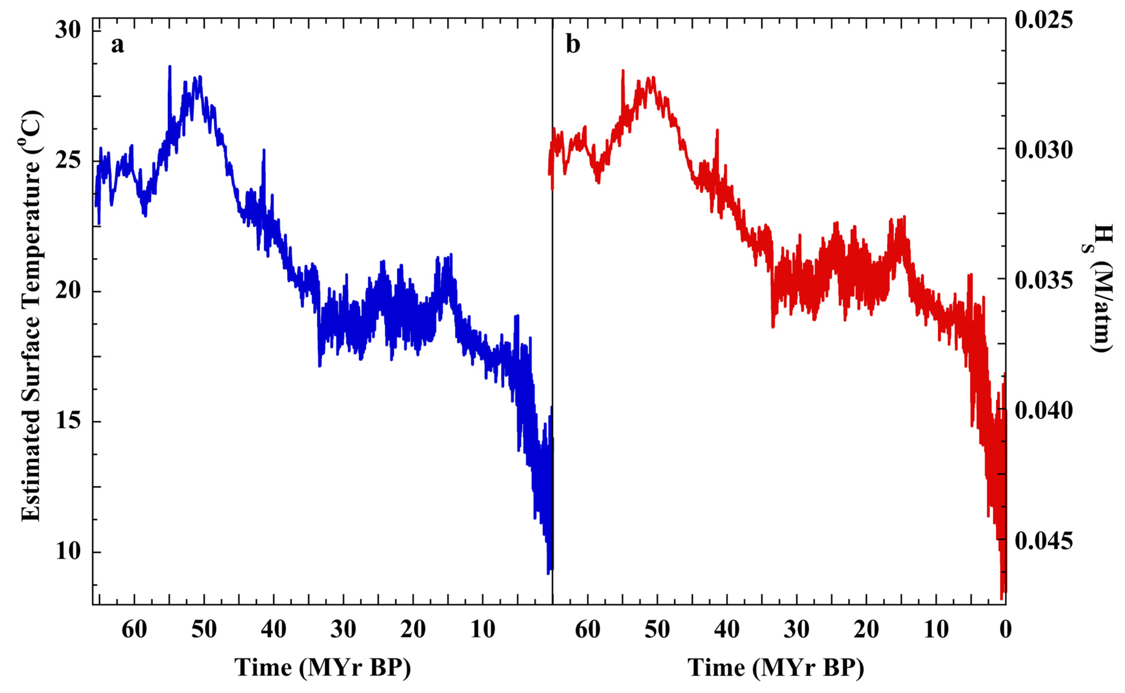
Figure 2.
(a) , (blue points); , (red line); , (black line); where P(CO2) is the historical atmospheric time series (ppm) since 1850. (b) (Blue line), Henry’s Law constant divided by the historical atmospheric CO2 time series plotted against CO2 (ppm). The structure reflects the impact of the natural variation of SST on the Henry’s Law constants (cf. hG in Equation (4)); (red line), linear least squares fit: H/P = 0.03779 − 8.466 × 10⁻⁶ × CO2 (ppm); r2 = 0.84. (c) , (red line), where P(CO2) is the historical record in ppm; (dashed red line), weighted fit through the data (see Sources and Methods Section); (blue line), slope = 1.00, where P is total pressure in atm, including seawater vapor pressure plus P(CO2) (cf. Equation (7): yi/xi = Hi/P).
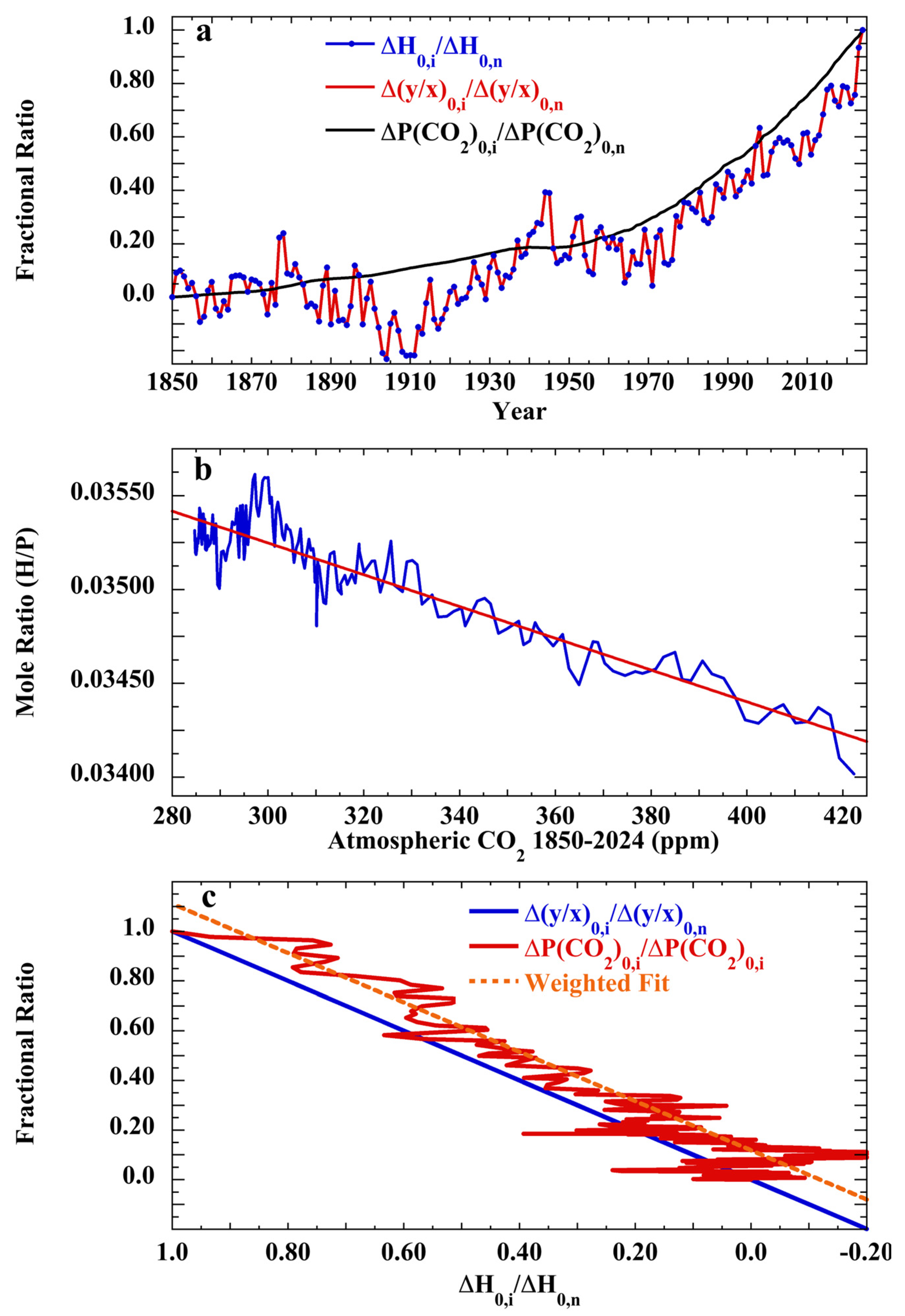
Figure 3.
(a) (Blue points), P(CO2) (ppm) as calculated under the Null Hypothesis (Equation (14)), with = 862 ppm and the fractional ratio of the temperature-varying Henry’s Law constant for seawater (Figure 1). The red line is a 1% weighted Lowess smooth. Inset (b): expansion of the most recent 7.5 Ma.
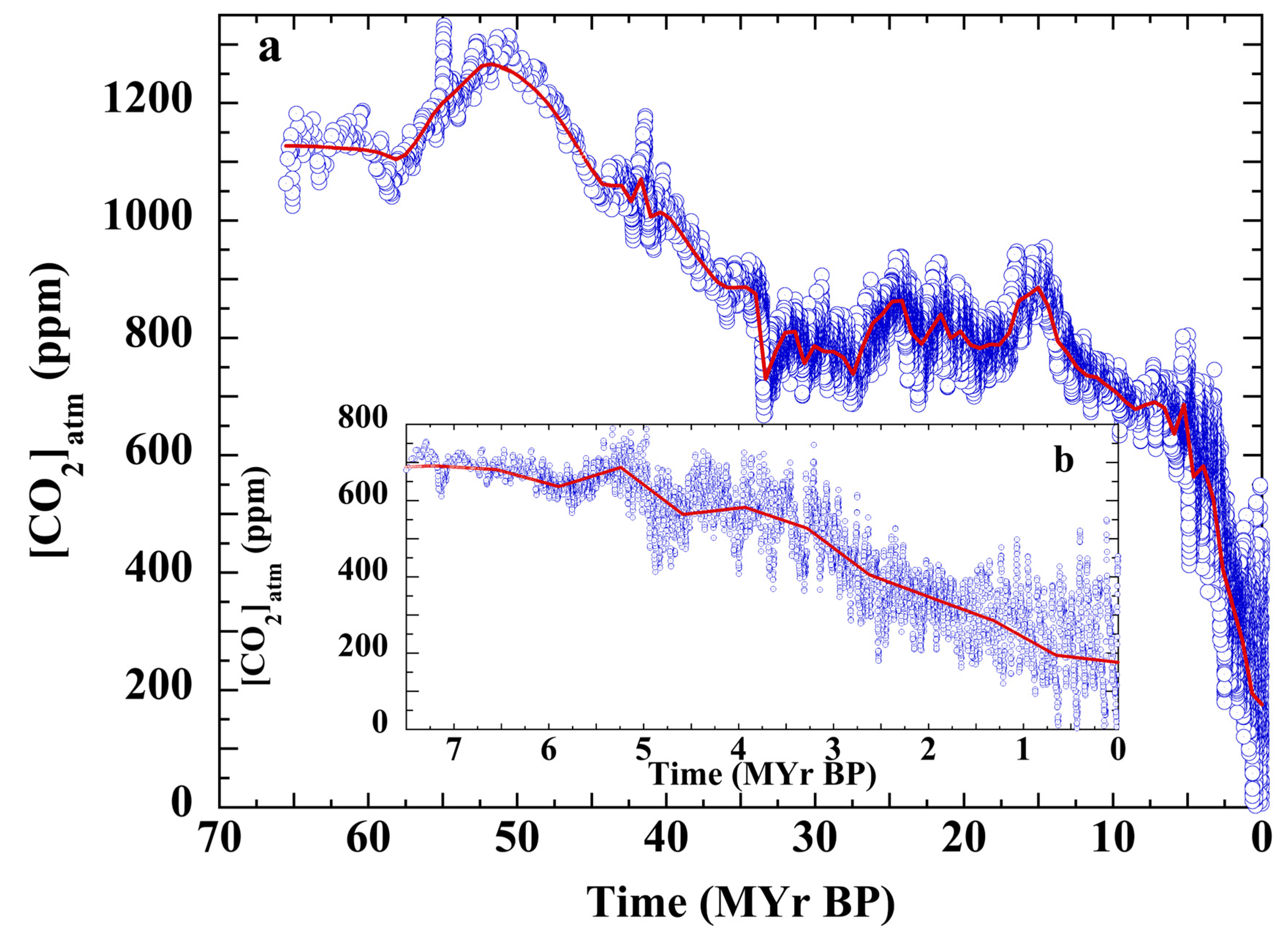
Figure 4.
(a) (Red line), Henry’s Law estimate of the evolution of atmospheric P(CO2) with varying SST and [CO2]ocean held constant at the initial Cenozoic concentration of 3.41 × 10⁻⁵ M; (blue line), Null Hypothesis estimate of the trend of P(CO2) constrained to the net proxy Cenozoic = 862 ppm. Inset (b): expansion of the first 25 Ma of the Cenozoic.
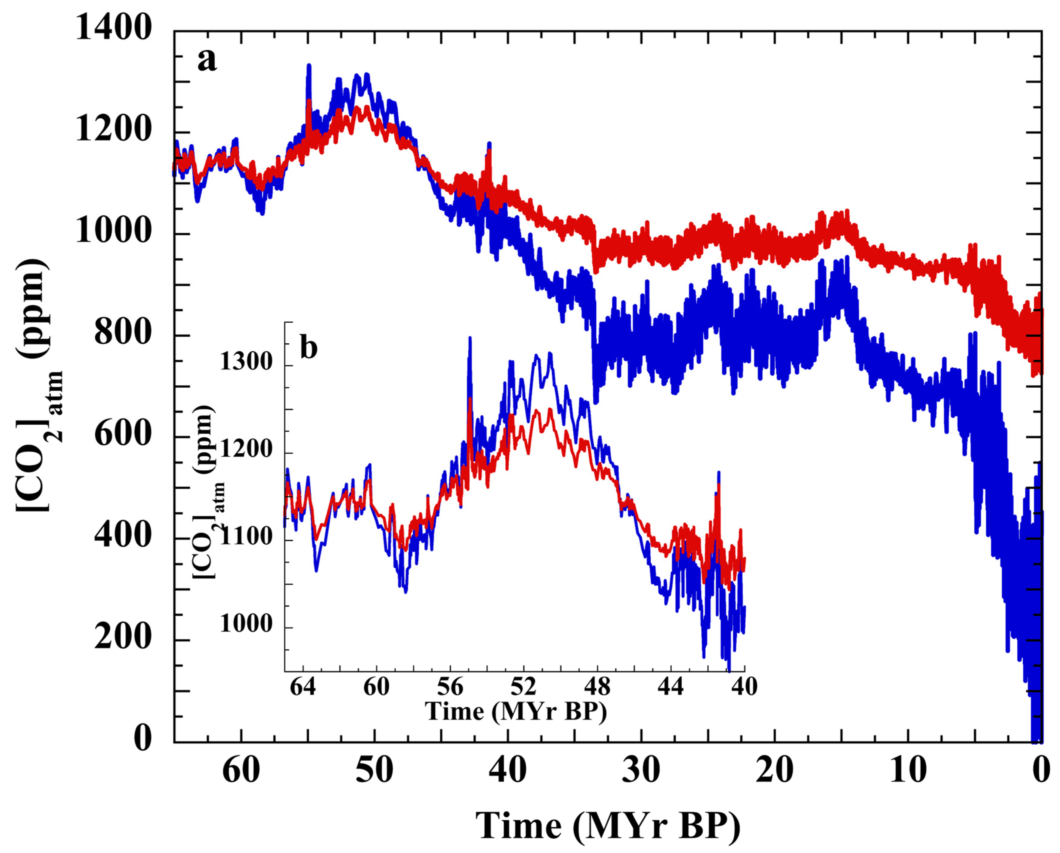
Figure 5.
(a) (Red line), Null Hypothesis estimate of the trend in atmospheric CO2 during the Cenozoic; (black line), a 1% weighted Lowess smooth of the estimate; (blue points), Cenozoic P(CO2) as estimated using marine core alkenone and boron isotope proxies [2]; and (blue line), a 5% weighted Lowess smooth of the proxy-derived trend in Cenozoic P(CO2). Inset (b): expansion of the most recent 7.5 Ma.

Figure 6.
(a) (Blue points), the Paleocene–Eocene proxy SST reconstruction of Bijl et al. (2009) [60]; (red line), the Hansen et al. (2013) proxy SST reconstruction [33]. The two reconstructions merge across 40 to 37 MYr BP. (b) (Pink points), proxy P(CO2) reconstruction of Rae et al. (2021), using marine core alkenone and boron isotope proxies [2]; (purple line), 5% weighted Lowess fit through the points of the proxy; (blue line), estimate of Cenozoic P(CO2) (ppm) calculated using Equation (14), including the PETM SSTs of Bijl et al. [60]; and (red line), piece-wise weighted Lowess fit to the Cenozoic CO2 estimate. The weights were 15% over the reconstruction of Bijl et al., (65–37 MYr BP) [60], and 1% over 37–0 MYr BP. Inset (c): expansion of the most recent 7.5 Ma.

Figure 7.
Double-y plot of the increase in P(CO2) during the MCO. (× points), proxy P(CO2) trend across the MCO [2]; (circular points plus black line), the proxy P(CO2) trend and the Lowess smooth (cf. Figure 4 and Figure 5); (red line), the Null Hypothesis estimate of SST-limited P(CO2) (cf. Figure 3); and (blue line), the Lowess smooth of the Null Hypothesis estimate. Both ordinates include a 550-ppm range but have been vertically offset so as to bring the two background slopes into coincidence.
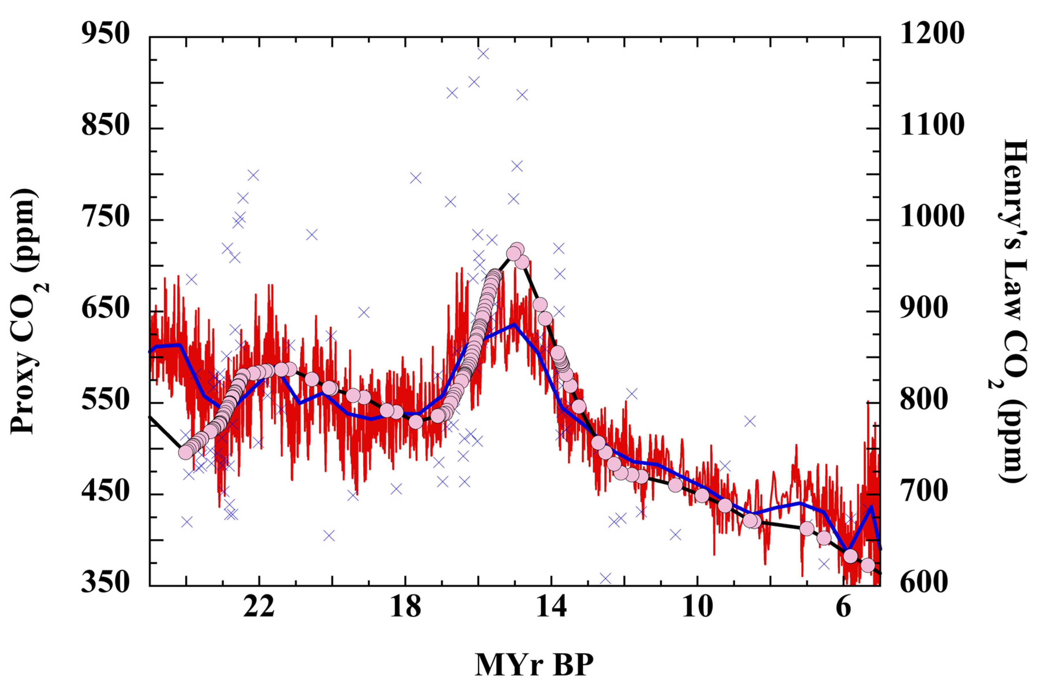
Figure 8.
(a) Henry’s Law constants for seawater reflecting the adjusted SSTs (see text). Note the descending ordinate. (b) (Red line plus points), VOSTOK ice core P(CO2) record; and (blue line), P(CO2) calculated using [CO2]ocean = 9.980 × 10⁻⁶ M and the adjusted HS reflecting an 11 °C glacial/interglacial temperature range (Equation (17)). (c) Method comparison: (blue line), replication of the VOSTOK P(CO2) calculated using the adjusted Henry’s Law constants (Equation (17)); and (orange line), VOSTOK P(CO2) calculated according to the Null Hypothesis using the ratio of adjusted HS values and the VOSTOK (Equation (18)). The two estimates express the assumption that the rises and falls of glacial/interglacial atmospheric P(CO2) reflect re-equilibrations across the sea surface driven by time-varying SST, alone.
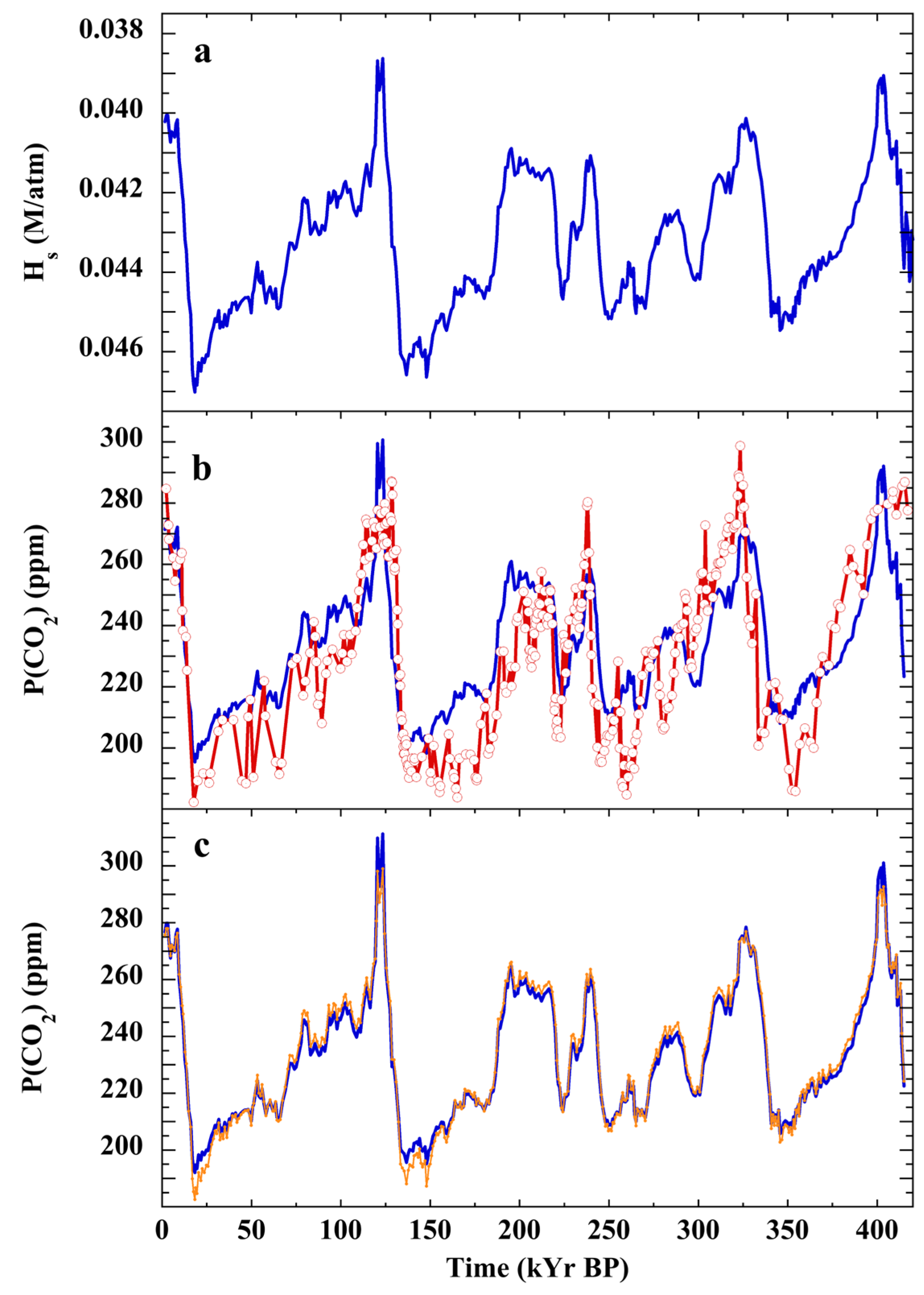

Table 1.
Salts used to approximate seawater of 35.1‰ salinity [56].
Table 1.
Salts used to approximate seawater of 35.1‰ salinity [56].
| Salt | NaCl | KCl | MgCl2 | MgSO4 | CaSO4 |
|---|---|---|---|---|---|
| Molality | 0.472 | 0.0103 | 0.0336 | 0.0196 | 8.82 × 10⁻³ |
| g/kg | 27.58 | 0.766 | 3.19 | 2.36 | 1.20 |
| Molarity | 0.456 | 0.0100 | 0.0324 | 0.0190 | 8.85 × 10⁻³ |
| Total mole fraction | 8.716 × 10⁻³ | 1.902 × 10⁻⁴ | 6.205 × 10⁻⁴ | 3.620 × 10⁻⁴ | 1.629 × 10⁻⁵ |
| Mole fraction of salts | 0.867 | 0.0189 | 0.0617 | 0.0360 | 0.0162 |
Total salinity: 35.1 g/kg = 35.1‰; total salt moles/kg = 0.544. Total mole fraction = (moles of salt)/(total moles) where total moles = (salts + water) = 54.150 moles/kg.
Table 2.
Schumpe parameters for major seawater ions.
| Anion | Schumpe hi | Cation | Schumpe hi |
|---|---|---|---|
| Cl− | 0.0318 | Na+ | 0.1143 |
| 0.1117 | K+ | 0.0922 | |
| Mg2+ | 0.1694 | ||
| Ca2+ | 0.1762 |
Ion-specific Schumpe parameters are available in Table 5.5 of Abbatt (2019) [44].
Disclaimer/Publisher’s Note: The statements, opinions and data contained in all publications are solely those of the individual author(s) and contributor(s) and not of MDPI and/or the editor(s). MDPI and/or the editor(s) disclaim responsibility for any injury to people or property resulting from any ideas, methods, instructions or products referred to in the content. |
© 2024 by the author. Licensee MDPI, Basel, Switzerland. This article is an open access article distributed under the terms and conditions of the Creative Commons Attribution (CC BY) license (https://creativecommons.org/licenses/by/4.0/).
Share and Cite
MDPI and ACS Style
Frank, P. Cenozoic Carbon Dioxide: The 66 Ma Solution. Geosciences 2024, 14, 238. https://doi.org/10.3390/geosciences14090238
AMA Style
Frank P. Cenozoic Carbon Dioxide: The 66 Ma Solution. Geosciences. 2024; 14(9):238. https://doi.org/10.3390/geosciences14090238
Chicago/Turabian StyleFrank, Patrick. 2024. "Cenozoic Carbon Dioxide: The 66 Ma Solution" Geosciences 14, no. 9: 238. https://doi.org/10.3390/geosciences14090238
Note that from the first issue of 2016, this journal uses article numbers instead of page numbers. See further details here.