Unraveling the Spatio-Temporal Evolution of the Ranchería Delta (Riohacha, Colombia): A Multi-Period Analysis Using GIS

Abstract

The Ranchería River delta, located in Riohacha, Colombia, exemplifies the complex dynamics of coastal systems influenced by environmental and anthropogenic factors. This study analyzes the spatial and temporal evolution of the delta’s shoreline over the past two decades (2003–2023) using Google Earth imagery, the Digital Shoreline Analysis System (DSAS) within a GIS environment, and statistical methods such as ANOVA and Tukey’s test. Satellite images from 2003 to 2023 were processed to evaluate shoreline evolution through metrics like the Net Shoreline Movement (NSM) and Linear Regression Rate (LRR). The results reveal a predominant trend of accretion, with values reaching up to 260 m of NSM, particularly between 2003 and 2018. However, the 2018–2023 period shows a shift toward stabilization and localized erosion (e.g., the NSM ranges from 96 m of erosion to 32 m of accretion), with significant changes in the northeastern area (the delta’s Santa Rita arm) attributed to anthropic and natural factors (e.g., absence of mangroves or ongoing human activities). The comparison of LRR and NSM values reveals consistent linearity in shoreline behavior across the study period, suggesting stable coastal processes during accretion-dominated phases and increased variability during recent erosion. Variability across zones highlights the role of natural barriers like mangroves in mitigating erosion. The findings underscore the importance of integrating long-term data with recent trends for shoreline management and emphasize adaptive strategies to conserve critical ecosystems while addressing the socio-economic needs of local communities.

1. Introduction

Coastal zones, including river deltas, hold critical importance, as they are home to approximately 40% of the global population (2.4 billion people) within a 100 km radius [1]. River deltas, defined as low-lying areas formed at the mouth of a river [2], are highly dynamic systems shaped by the interplay of fluvial, marine, and anthropogenic processes [3]. These vulnerable ecosystems face increasing challenges from human activities and climate change, which significantly impact both their morphology and functionality.

Examples such as the Nile Delta, where protective coastal structures like groins and breakwaters have been implemented, illustrate how human interventions can mitigate erosion in specific areas while accelerating it in others [4]. Similarly, in the Küçük Menderes Delta (Türkiye), the construction of the Burgaz Dam in 2018 increased erosion rates by disrupting sediment flow [5]. In contrast, the São Francisco River Delta (Brazil) has experienced erosion since 1985, driven more by hydrological changes caused by river regulation and climate change (reduced rainfall in the basin) than by sediment retention from dams [6]. These cases underscore the inherent complexity of delta dynamics, influenced by multiple interacting factors.

The analysis of shoreline changes has emerged as a research field of increasing importance. For instance, Rahman et al. [7] reported a significant rise in related recent scientific publications, with 371 studies indexed between 2019 and 2022. This growth reflects the urgency to address challenges related to shoreline dynamics, which are essential for understanding erosion, sedimentation, and geomorphological changes (e.g., river mouth displacement or variation in altitude in selected areas of the delta) in coastal zones. Historically, these studies relied on traditional cartography and terrestrial surveys [8] and the extraction of shorelines from aerial photographs. While precise, these techniques have limitations in terms of cost and spatiotemporal coverage. Remote sensing technologies and Geographic Information Systems (GIS) have revolutionized coastal analysis by leveraging satellite imagery such as Landsat and Sentinel, offering high temporal and spatial resolution at a lower cost and with greater efficiency [9,10]. The integration of multifaceted data sources, including optical and radar imagery, has significantly enhanced monitoring in challenging conditions like persistent cloud cover or extreme events. These technologies enable detailed analysis of erosion and accretion trends and assess the impact of human activities and climate phenomena on shorelines [11], particularly useful for large-scale studies. Some studies have been limited by temporal coverage and spatial scale, often relying on field surveys that are complemented by satellite or aerial imagery. However, these approaches typically face constraints in terms of long-term data availability and the spatial resolution required to fully capture coastal dynamics [12]. Furthermore, satellite imagery often requires correction using ground-truth data, which can be challenging in remote or resource-limited areas where access is difficult and financial or material resources are scarce [13].

Moreover, advancements in machine learning algorithms, including neural networks, are transforming coastal monitoring by identifying shoreline changes with high precision, even under adverse climatic conditions [14]. Despite their efficiency and scalability, automated methodologies face limitations in detecting intricate coastal features, making them less suitable for studies focused on areas requiring high spatial detail and precision, where complementary field observations may be useful [15,16]. In this context, the Digital Shoreline Analysis System (DSAS) has become a central tool for analyzing coastal dynamics. DSAS, which operates within GIS environments, allows for the calculation of key metrics that are particularly useful for long-term studies, combining historical data with recent satellite imagery to identify erosion and accretion patterns [17]. Recent studies have applied DSAS in diverse coastal settings, demonstrating its effectiveness in assessing and managing areas vulnerable to climate change and evaluating anthropogenic impacts [15,16,17,18,19,20].

Within a global framework, the coastal dynamics of La Guajira Department (Guajira Peninsula, Colombian Caribbean), where the Ranchería River delta is located, have been highly sensitive to environmental changes and human activities in recent decades [21,22]. The Ranchería Delta, in particular, experiences strong coastal dynamism driven by variable fluvial processes. River discharge fluctuates from near zero for most of the year to significant flooding during the rainy season, causing rapid morphodynamic changes such as sedimentation, channel closure, and periodic coastal bar formation, which obstructs river mouths and triggers local flooding. Human interventions, particularly coastal defense structures like groins near the delta, may have further altered sediment dynamics over the past two decades [23]. While these modifications have shaped coastal morphology in the short and medium term, their long-term implications remain uncertain, highlighting the need for a multi-period approach to capture shoreline evolution at different time scales. Many coastal studies focus on a single observation period, limiting the identification of long-term trends and variability [24]. However, dynamic environments like the Ranchería Delta require a more comprehensive approach that integrates multiple temporal perspectives. Analyzing its evolution across multiple timeframes allows for a deeper understanding of its interactions with natural and human processes, essential for effective coastal management.

This study enhances the understanding of coastal morphodynamic changes in dynamic, vulnerable, and protected areas facing socio-environmental challenges such as poverty and climate change. This research develops a temporal analysis framework to evaluate the spatio-temporal evolution of coastal erosion and accretion patterns in the Ranchería River delta, focusing on the dominant trends in the region. Specifically, this research quantifies and analyzes shoreline changes in the delta over the past two decades using satellite imagery from multiple time periods. To achieve this, geospatial analysis tools and specialized metrics have been applied through software such as ArcGIS v. 10.5, ArcGIS Pro v. 3.1.3, and DSAS v. 5.1, enabling a detailed assessment of spatial and temporal shoreline evolution.

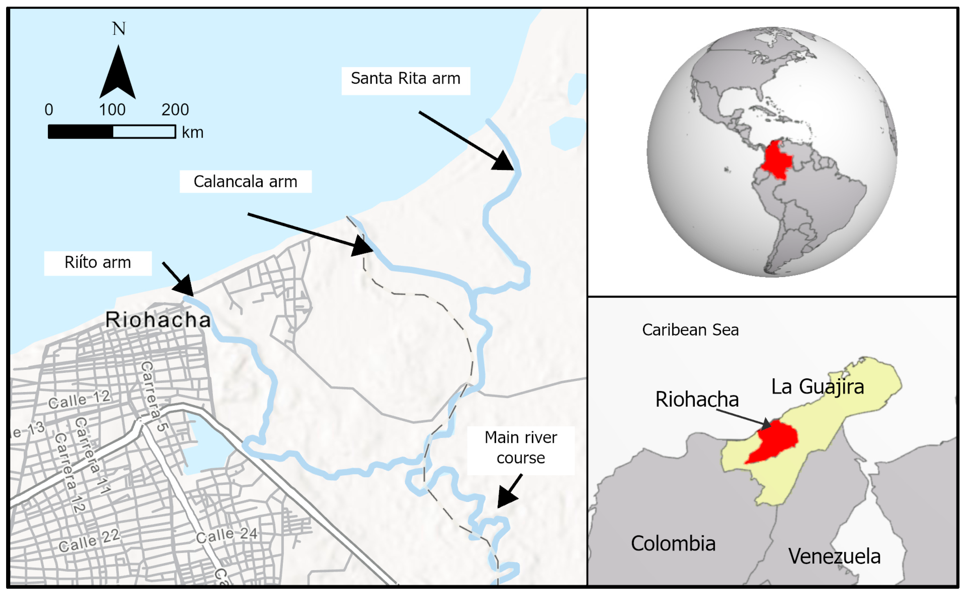
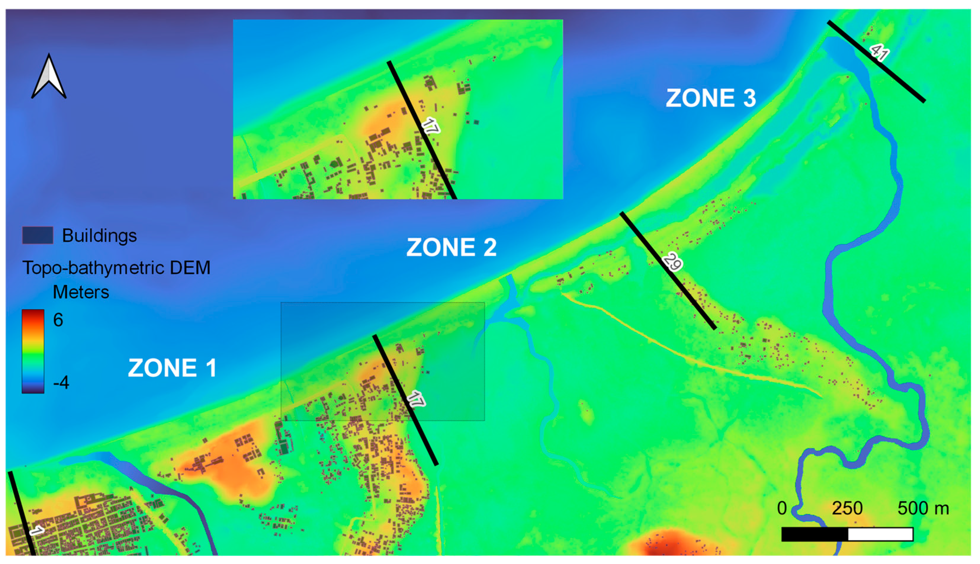
2. Study Site Description

The study site is in the delta of the Ranchería River, which flows into the Caribbean Sea near Riohacha in La Guajira, Colombia (Figure 1). This region features low-lying flat terrain with dynamic interactions between fluvial and marine processes. Originating in the Sierra Nevada de Santa Marta, one of the highest coastal mountain ranges globally, the Ranchería River traverses arid landscapes before reaching the delta. As it enters the coastal plain near Riohacha, the river is influenced by the Caribbean Low-Level Jet, which induces coastal upwelling along the Guajira coast [25]. The area’s sediments are predominantly alluvial, underlain by aeolian deposits, and the gently undulating coastal plain is fed by sediment from Ranchería River. At the river’s mouth, a seasonal estuary forms during the brief rainy season [26].

The region experiences a semi-arid to arid climate, with average annual rainfall of approximately 550 mm [27], most of which occurs during a brief rainy season from September to November. The Ranchería River is the primary freshwater source for many dispersed rural and indigenous settlements in Riohacha and surrounding areas, although its flow has been heavily regulated by the El Cercado Dam (built in the mid-2000s) upstream. The hydrology of the delta has thus been influenced by both seasonal rainfall and anthropogenic factors, which affect freshwater flow and sediment delivery to the delta. In the Colombian Caribbean region, tidal patterns are characterized by mixed semidiurnal cycles with micromareal influence, resulting in low amplitude tides that average around 0.3 m and can reach up to 0.65 m during peak conditions [28]. Successive high tides occur approximately every 11.5 h, though intervals can vary from 10 to 14 h [28]. The prevailing swell in the region is driven by climatological factors, with a dominant northeast–southwest (NE–SW) direction from November to July and peak wave heights of 4.5 to 5 m. From August to October, the swell shifts to a southwest–northeast (SW–NE) orientation, with reduced wave heights of up to 1.5 m [29,30].

The delta encompasses a mosaic of ecosystems, including mangroves, estuarine wetlands, and coastal dunes. These habitats are crucial for biodiversity, supporting a variety of fish species, crustaceans, and migratory bird populations. Mangroves in particular play a vital role in protecting the coastline from erosion, regulating water quality, and providing habitat for juvenile marine species [27]. However, these ecosystems are under threat due to factors like sediment budget alteration, urban encroachment, and changes in salinity.

The Ranchería River delta is central to the livelihoods of local communities, including the indigenous Wayuu people, who depend primarily on fishing and small-scale agriculture. However, the area faces significant socio-economic challenges, including water scarcity, limited access to public services, and vulnerability to natural hazards. Moreover, the regulation of water flow due to damming (El Cercado Dam) has altered sediment transport dynamics, potentially leading to habitat degradation [31]. Additionally, Riohacha, the department capital, is undergoing rapid urban expansion, placing pressure on natural resources and altering land use patterns in the delta. Conservation of the delta’s ecosystems is vital not only for biodiversity but also for maintaining the ecosystem services upon which local communities depend.

3. Methodology

The methodological workflow for assessing shoreline evolution and its spatiotemporal variability in the Ranchería River delta, outlined in Figure 2, comprises several steps, which are detailed in this section: (1) image acquisition and preprocessing, (2) reprojecting and spatial accuracy, (3) shoreline profiling, (4) baseline construction and data structuring, (5) casting transects, and (6) temporal trends in shoreline change metrics.

3.1. Image Acquisition and Preprocessing

The process began with the selection, downloading, and preprocessing of satellite images for the study area, ensuring their consistency for subsequent geospatial analysis. This study used eight aerial images from Google Earth Pro (2024) [32], corresponding to the years 2003, 2006, 2009, 2014, 2018, 2020, 2021, and 2023. Google Earth imagery was chosen due to its availability over an extended temporal range and its sufficient spatial resolution for detecting shoreline changes at the scale of tens of meters. While alternatives such as Sentinel-2 or UAV imagery offer higher spectral consistency, they do not provide a continuous historical record with the necessary temporal coverage for long-term shoreline evolution studies in this region.

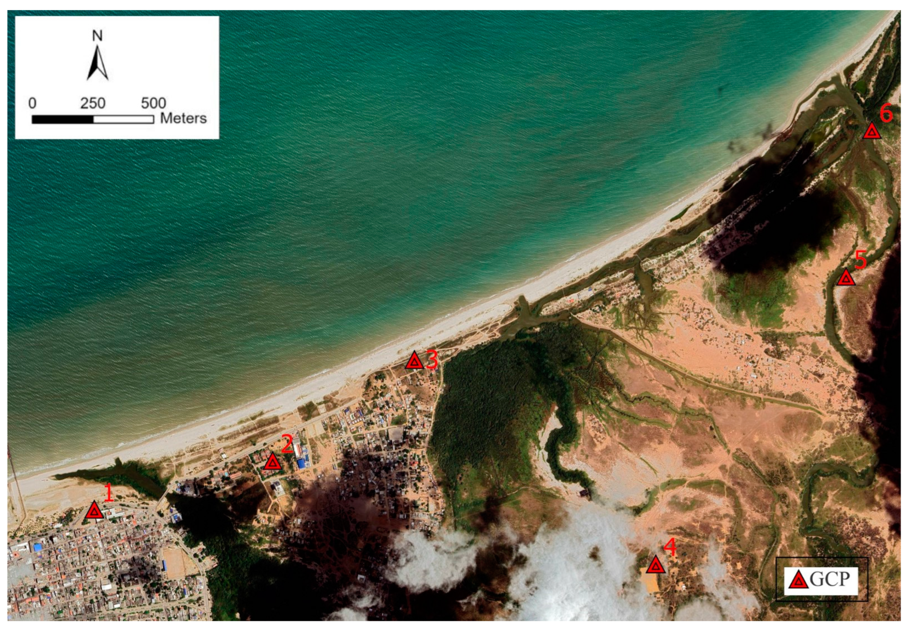
3.2. Reprojecting and Spatial Accuracy

These images, while containing geospatial information based on the WGS84 reference system, often require reprojecting to ensure their precision and suitability for spatial analysis. Misalignments or geometric distortions can occur due to various factors, such as projection discrepancies, sensor errors, or distortions introduced during image acquisition. Reprojecting is a critical process to address these inconsistencies, aligning the images to a standardized coordinate system—WGS 1984 UTM Zone 18N in this case—and ensuring spatial coherence among multiple images used for multi-temporal analyses. This step is essential for enabling accurate measurements.

Once downloaded, the images were imported into separate layers within ArcGIS Pro 3.1.3 [33]. Among the available images, the most recent (from 2023) was selected as the reference image for reprojecting the others. This process utilized six ground control points (GCPs) for each image, ensuring proper spatial alignment (see Figure 3). The selected GCPs were strategically distributed across the images, ensuring a robust transformation that minimized spatial distortions and maintained shoreline alignment consistency across all years. To ensure accuracy and reliability, the control points were chosen in stable unaltered areas, preferably where permanent constructions were present, as these provide consistent and easily identifiable markers. The identified points were readily discernible in the urban region situated in the western section of the images, which has undergone minimal change over the past 20 years. Conversely, in the eastern and southern areas, where indigenous communities reside, pinpointing stable locations has proven significantly more challenging due to the fluctuations in human settlements that have occurred during this timeframe. For the reprojecting process, a projective transformation was applied. This transformation preserves straight lines but not necessarily parallelism or angles. The careful selection of control points, combined with a robust transformation model, contributed significantly to the spatial accuracy of the dataset.

The georeferencing process resulted in varying RMSE (Root Mean Square Error) values across different years, reflecting differences in image quality and geolocation accuracy. The RMSE is a quantitative metric used to assess the accuracy of image alignment with the reference system. It is calculated as the square root of the mean of the squared residual errors, which are determined as the Euclidean distance between the transformed source coordinates and the corresponding reference coordinates across all control points. This method ensures a consistent spatial framework across all images, which is crucial for shoreline change analysis and multi-temporal comparisons. The highest RMSE was observed for the 2006 image (8.87 m), likely due to lower positional accuracy and resolution in older satellite data. In contrast, the 2023 image, which served as the reference, had the lowest RMSE (0.77 m), benefiting from advancements in remote sensing technology. The remaining images exhibited intermediate RMSE values, ranging from 1.06 m (2020) to 4.03 m (2014), with most values remaining below 2.5 m, indicating an overall high level of georeferencing accuracy. While RMSE values varied across years due to differences in image resolution and sensor accuracy, these variations are minimal relative to the magnitude of observed shoreline changes, which occur at scales of tens to hundreds of meters. Additionally, the limited availability of stable reference points in the study area—characterized by minimal built infrastructure—posed challenges for georeferencing, particularly in older images. Despite these constraints, the applied methodology ensures spatial consistency. Given the flat nature of the delta, any potential vertical inaccuracies do not significantly impact shoreline positioning.

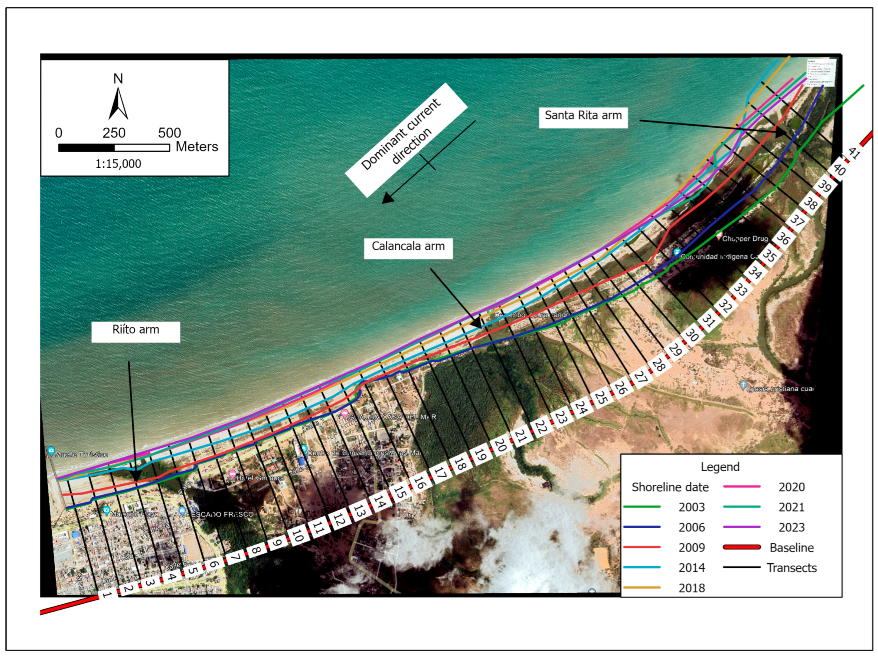
3.3. Shoreline Profiling

Once the images were reprojected, the next step involved determining the position of the shoreline with the highest possible precision [5]. Shoreline position can be identified using various indicators, such as the low tide line, mean tide line, high tide line, or maximum storm surge line, among others. For this study, the High-Water Line (HWL) was selected as the reference across all images. The HWL is identified by the visual contrast between dry sand (lighter tones) and wet sand (darker tones), providing a clear and consistent boundary for delineation [34]. Given the spatial extent of the study area and the resolution of the available data, a manual digitization approach was adopted to extract the shorelines. Manual digitization, although time-intensive, ensures greater accuracy in cases where the shoreline features are complex or where automated methods may struggle to differentiate subtle contrasts. This approach is particularly advantageous for medium-scale studies where precision is prioritized over efficiency [4,35].

3.4. Baseline Construction and Data Structuring

These steps are necessary for the DSAS v. 5.1, an ArcGIS extension developed by the United States Geological Survey (USGS) [17], to process the data and generate outputs. The construction of the baseline is a fundamental step in coastal analysis and can be achieved through various approaches according to the DSAS User Guide. These include manual digitization, applying smoothing or buffering techniques to an existing line, or utilizing a pre-existing baseline. In this study, the 2018 baseline was chosen as it represents an intermediate position between the study periods, providing a balanced reference for shoreline evolution analysis. The baseline was generated to follow the general orientation of historical shorelines, ensuring consistency in shoreline change analysis [36]. To refine its geometry and improve its accuracy, a smoothing process was applied using the Smooth Tool in ArcGIS v.10.5 [37], eliminating sharp angles and enhancing the continuity of the line. The smoothing technique is the most dependable and accurate method for delineating baselines [10,38]. Following established methodologies for baseline generation, the finalized baseline was positioned slightly inland. This placement was chosen to minimize distortions in transect orientation and maintain a stable reference for measuring coastal evolution. To ensure compatibility and functionality, both the baseline and the shoreline layers require specific attributes in their respective attribute tables. These attributes must be manually defined by the user. For the baseline, the attribute table must include a mandatory ID field, which is essential for sequencing and organizing transects, particularly when the baseline comprises multiple segments. Importantly, the ID attribute cannot have a value of zero, as this could lead to processing errors. Similarly, the shoreline layer must include a DATE attribute, formatted as MM/DD/YYYY, to record the acquisition date of each shoreline. Once the baseline and shoreline layers are properly configured, they must be stored together in a single personal geodatabase. The geodatabase serves as the repository for both the input layers and the results of the analysis. Ensuring that the layers are correctly formatted and contain the required attributes is crucial for the successful implementation of the DSAS workflow.

3.5. Casting Transects

Once the shoreline and baseline layers are integrated into a single personal geodatabase, the process of generating the transect layout can begin. Using DSAS, transects are automatically generated as lines extending perpendicularly from the baseline and spaced at uniform intervals. For this study, a transect spacing of 100 m was selected to ensure a representative and consistent analysis of shoreline changes along the 4.3 km stretch of coastline. This interval provides a balance between capturing localized variations and maintaining a clear, large-scale trend without excessive redundancy for a smooth coastline like the one studied [34,39]. As a result, 41 transects were generated, offering sufficient resolution to detect meaningful patterns of erosion and accretion while minimizing potential spatial autocorrelation. These transects serve as the initial elements for subsequent shoreline change analysis, including the application of linear regression models to quantify rates of erosion and accretion.

3.6. Temporal Trends in Shoreline Change Metrics: Multi-Period Statistical Analysis (2003–2023)

In this study, the spatial and temporal distribution of shoreline changes has been analyzed by dividing the dataset into three periods (2003‒2018, 2018‒2023, and 2003‒2023). Shoreline changes were evaluated using several metrics derived from the DSAS tool: Net Shoreline Movement (NSM), End Point Rate (EPR), and Linear Regression Rate (LRR). The NSM measures the distance, in meters, between the oldest and most recent shoreline along each transect. The EPR is calculated by dividing the NSM by the time elapsed between the oldest and most recent shorelines used for the calculation, and it is expressed in meters per year. The LRR represents the slope of a least-squares linear regression fitted to all shoreline positions along each transect, with the slope indicating the rate of shoreline change (erosion or accretion) in meters per year. The values obtained for the LRR at each transect (or set of transects) can be categorized following the classification of Natesan et al. [40] and summarized in

Table 1. Classification of LRR (m/yr) erosion/accretion values.

Category	Shoreline Change Rate Intervals	Shoreline Rate Classification
1	LRR < −2	Very high erosion
2	−2 < LRR < −1	High erosion
3	−1 < LRR < 0	Moderate erosion
4	LRR = 0	Stable
5	0 < LRR < 1	Moderate accretion
6	1 < LRR < 2	High accretion
7	LRR > 2	Very high accretion

. It is important to emphasize that both the LRR and the EPR are parameters that help measure the rate of shoreline change (therefore, they can be considered equivalent parameters), while the NSM quantifies the net change of the shoreline.

DSAS also provides supplementary statistics to evaluate the reliability of the LRR. These include the Linear Regression Confidence Interval (LCI) and the Coefficient of Determination (LR2). The LCI, calculated at a 99% confidence level, represents the range within which the true LRR is expected to fall. It quantifies the uncertainty associated with the LRR estimation and is expressed in meters per year. A narrower LCI indicates higher confidence in the regression model, whereas a wider LCI suggests greater variability or uncertainty in the LRR. The LR2 value, derived from the linear regression model, represents the proportion of variance in the shoreline position explained by the regression. It ranges from 0 to 1, where values closer to 1 indicate a better fit and a stronger correlation between time and shoreline change. For more details, see the DSAS User Manual [17]. Based on this parameter, and following the idea of Sabour et al. [41], it is possible to categorize the transects as strongly linear (LR2 > 0.7), weakly linear (0.3 < LR2 < 0.7), or non-linear (LR2 < 0.3). Additionally, to assess whether the changes in the delta shoreline are statistically significant, a two-way analysis of variance (ANOVA) [42] was performed using MATLAB R2023b [43]. This test can be applied to the following metrics: NSM, EPR, or LRR. If significant differences are detected, Tukey’s test [44] is then applied to identify where and when these differences occur. This post-hoc test is appropriate for multiple pairwise comparisons and ensures that the differences detected are statistically reliable.

4. Results

This study has been divided into three temporal periods to obtain detailed shoreline change statistics and behaviors. A long-term period includes all available years with data (2003–2023), capturing the full variability of the study area. Additionally, two shorter periods, 2003–2018 and 2018–2023, were defined to obtain detailed shoreline change statistics and tendencies. Figure 4 shows the position of the shorelines at different times (from 2003–2023) with respect to the baseline and the 41 transects plotted along the Delta.

4.1. Shoreline Change Metrics: Trends in Accretion and Erosion

All transects during the full study period (2003–2023; see

Table 2. Values and rates of change of the shoreline according to the analysis extracted with DSAS software for the three time periods.

Statistics	2003–2018	2018–2023	2003–2023
Total number of transect	41	41	41
NSM (m)
Average	165.71	4.50	170.21
Minimum	41.66	−95.91	64.92
Maximum	322.33	32.26	260.08
Standard Deviation	80.13	35.87	53.30
EPR (m/yr)
Average	11.05	0.84	8.37
Minimum	2.78	−17.98	3.19
Maximum	21.49	6.05	12.79
Standard Deviation	5.34	6.72	2.62
LRR (m/yr)
Average	11.79	0.65	9.33
Minimum	2.51	−18.31	3.58
Maximum	22.96	6.29	14.49
Standard Deviation	5.86	6.97	2.86
LR2
Average	0.94	0.76	0.91
Minimum	0.65	0.18	0.57
Maximum	0.99	1	0.98
Standard Deviation	0.06	0.21	0.09
Erosion Transects, Number	0 (0%)	10 (24%)	0 (0%)
Accretion Transects, Number	41 (100%)	31 (76%)	41 (100%)
Overall trend of the period	Accretion	Accretion	Accretion

) showed LRR values >2, classifying them as having very high accretion (Table 1). This pattern is primarily attributed to the 2003–2018 period, during which all transects exhibited accretion with positive EPR values. In contrast, for the 2018–2023 period, the percentage of transects with very high accretion decreased to 73%, with 3% showing high accretion (category 6—Table 1). Additionally, nine transects (22%) exhibited very high erosion (category 1—Table 2), and one transect showed high erosion (2%). During this period, the NSM values were significantly lower, accompanied by a decrease in EPR values.

Regarding net shoreline movement (NSM—Table 2), the average value between 2003 and 2018 was considerably high (165.71 m). However, during the 2018–2023 period, the NSM decreased substantially to 4.50 m. In Figure 5, the 2003–2023 period (shown in blue) displays significant accretion values, reaching a minimum around transects 15 to 17. From T18 onwards, accretion values increase sharply. In contrast, the 2018–2023 period (shown in purple) remains relatively stable, with shoreline growth around 15 m up to T11 and increasing to values between 25 and 30 m up to T31. Beyond T31, NSM trends shift, showing notable erosion (negative values).

When analyzing shoreline change rates (understood as change velocity), the EPR for the 2003–2018 period was 11.05 m/yr, while the LRR was 11.79 m/yr, with both values being very similar. The strong goodness of fit during this period reflects relatively stable coastal dynamics, with a clear accretion trend accurately captured by the linear model (49 transects classified as strongly linear and only one as weakly linear). In contrast, for the 2018–2023 period, both rates declined sharply (EPR: 0.84 m/yr; LRR: 0.65 m/yr). This period exhibits less linearity, with 28 transects classified as strongly linear, 10 as weakly linear, and three as non-linear (T3, T30, and T31). The decrease in LR2 indicates greater variability in shoreline change patterns. Considering the full period (2003–2023), the trend returns to being highly linear (LR2 = 0.91; see Table 2), with 39 transects classified as strongly linear and only two as weakly linear. Therefore, it can be concluded that the EPR and LRR exhibit similar behavior across all analyzed periods, highlighting the linearity of shoreline evolution. As a direct consequence, the analysis can focus on just one of these indicators.

The correlation between the NSM and LRR provides valuable insight into shoreline dynamics, helping to identify areas where erosion is most pronounced. Sectors displaying both low (or negative) LRR values—indicating a long-term trend of retreat—and negative NSM values—reflecting net shoreline movement landward—are particularly vulnerable to erosion. These areas may require targeted mitigation measures to prevent further coastal retreat and minimize potential impacts. Figure 6 shows a strong correlation between these two parameters across the three periods, suggesting again that shoreline changes follow a consistent linear pattern over time (as other authors reflect [45]). In the 2018–2023 period, there is clear evidence of a general trend shift, particularly in the final transects (Santa Rita arm mouth area; Figure 4). Therefore, the roles of the NSM and LRR are analyzed in detail and separately, considering different temporal intervals and the spatial distribution of the transects.

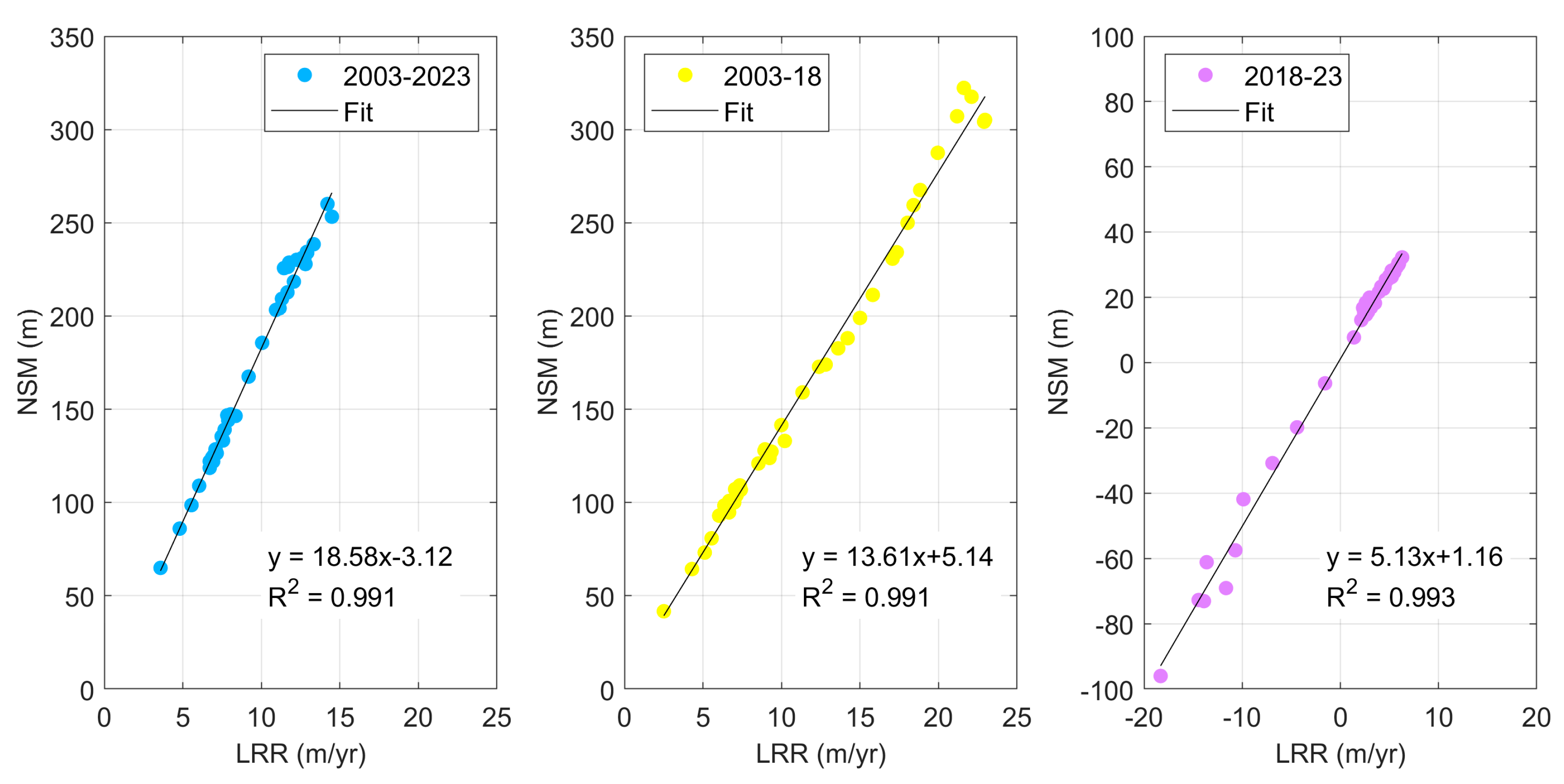
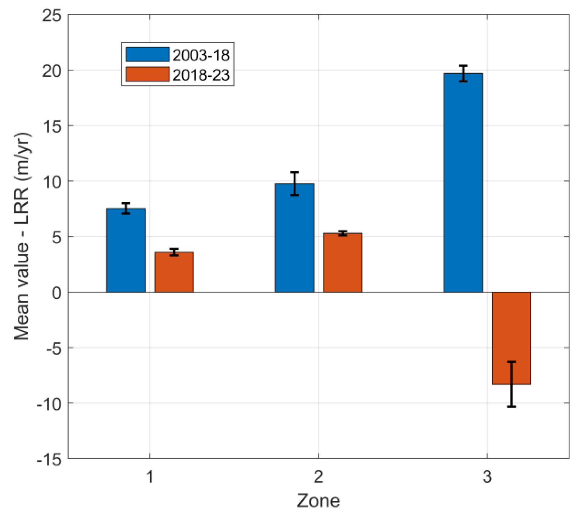
4.2. Spatial and Temporal Patterns of Shoreline Change and Statistical Significance

Based on the results from Section 4.1, the study area was divided into three zones: zone 1 includes transects 1 to 17, corresponding to the urban area of Riohacha or the Riito arm (Figure 4 and Figure 7); zone 2 comprises transects 18 to 29, covering the Calancala mouth area and the Cangrejito indigenous community (Figure 4 and Figure 7); and zone 3 includes transects 30 to 41, corresponding to the Santa Rita arm mouth area (Figure 4 and Figure 7).

4.2.1. Net Shoreline Movement (NSM)

Using a two-way ANOVA (time intervals and geographical distribution), it is demonstrated that the time interval (2003–2018 vs. 2018–2023) has a significant effect on the NSM parameter (p-value < 0.05;

Table 3. Two-way ANOVA results for the effects of the independent variables, time interval (Period) and Zone (1, 2, or 3), on the dependent variable, NSM. The table includes: Source (tested variable), Sum of Squares (total variation), Degrees of Freedom (independent data points), Mean Sum of Squares (Sum of Squares divided by Degrees of Freedom), F-statistic (ratio of Mean Sum of Squares of the factor to the residual), and p-value (statistical significance at $\alpha =0.05$).

Source	Sum of Squares	Degrees of Freedom	Mean Sum of Squares	F	p-Value
Period	5.89 × 105	1	5.89 × 105	686.97	8.27 × 10−40
Zone	3.79 × 104	2	1.89 × 104	22.11	2.71 × 10−8
Period:Zone	2.05 × 105	2	1.03 × 105	119.65	3.31 × 10−24
Error	6.51 × 104	76	8.57 × 102
Total	8.41 × 105	81

). The variability explained by the three zones is lower than that explained by the period but is also statistically significant.

To determine the specific effect of the interactions between zones and time periods, Tukey’s test was applied (see Figure 8). The general trend in zones 1 and 2 shows a significant decrease in net accretion. Additionally, zones 1 and 2 do not exhibit significant differences between each other for each period, with a p-value of 0.16 during 2003–2018 and a p-value of 0.98 during 2018–2023. In contrast, zone 3 shows a significant variation between the two time periods (2003–2018 and 2018–2023), indicating a shift in the coastal dynamics of this area, from a notable shoreline advance during 2003–2018 to a marked retreat in 2018–2023.

4.2.2. Linear Regression Rate (LRR)

The analyzed time periods, 2003–2018 and 2018–2023, also show significant differences in the LRR (

Table 4. Two-way ANOVA results for the effects of the independent variables, time interval (Period) and Zone (1, 2, or 3), on the dependent variable, LRR. The table includes: Source (tested variable), Sum of Squares (total variation), Degrees of Freedom (independent data points), Mean Sum of Squares (Sum of Squares divided by Degrees of Freedom), F-statistic (ratio of Mean Sum of Squares of the factor to the residual), and p-value (statistical significance at $\alpha =0.05$).

Source	Sum of Squares	Degrees of Freedom	Mean Sum of Squares	F	p-Value
Period	2.97 × 103	1	2.97 × 103	267.84	0
Zone	6.52 × 101	2	3.26 × 101	2.94	0.0591
Period:Zone	2.41 × 103	2	1.20 × 103	108.45	0
Error	8.43 × 102	76	1.11 × 101
Total	5.86 × 103	81

). Although the geographical factor (or zone) exhibited variations among the three study areas, this effect was not statistically significant (p-value = 0.0591), suggesting that the differences between zones are not sufficiently marked to be statistically relevant when the temporal factor is disregarded. However, the interaction between period and zone was highly significant (p-value < 0.001), indicating that the effect of the period (2003–2018 vs. 2018–2023) on the LRR depends on the study zone.

Tukey’s test (Figure 9 and

Table 5. Tukey’s test for significant variations of LRR along different periods and zones.

Source of Variation	Lower Limit	Upper Limit	p-Value
Zone 1 (2003–2018) vs. Zone 1 (2018–2023)	0.49	7.37	0.0157
Zone 1 (2003–2018) vs. Zone 2 (2003–2018)	−1.40	5.87	0.4746
Zone 1 (2003–2018) vs. Zone 2 (2018–2023)	−5.87	1.40	0.4743
Zone 1 (2003–2018) vs. Zone 3 (2003–2018)	8.43	15.87	1.62 × 10−13
Zone 1 (2003–2018) vs. Zone 3 (2018–2023)	−19.55	−12.11	6.06 × 10−19
Zone 1 (2018–2023) vs. Zone 2 (2003–2018)	2.53	9.81	6.01 × 10−5
Zone 1 (2018–2023) vs. Zone 2 (2018–2023)	−1.93	5.33	0.7455
Zone 1 (2018–2023) vs. Zone 3 (2003–2018)	12.37	19.81	2.58 × 10−19
Zone 1 (2018–2023) vs. Zone 3 (2018–2023)	−15.61	−8.17	4.00 × 10−13
Zone 2 (2003–2018) vs. Zone 2 (2018–2023)	0.65	8.29	0.0125
Zone 2 (2003–2018) vs. Zone 3 (2003–2018)	6.02	13.82	1.90 × 10−9
Zone 2 (2003–2018) vs. Zone 3 (2018–2023)	−21.96	−14.16	6.37 × 10−21
Zone 2 (2018–2023) vs. Zone 3 (2003–2018)	10.49	18.29	7.13 × 10−16
Zone 2 (2018–2023) vs. Zone 3 (2018–2023)	−17.50	−9.69	9.55 × 10−15
Zone 3 (2003–2018) vs. Zone 3 (2018–2023)	24.01	31.96	1.60 × 10−34

) was performed to identify significant differences between the zones and periods. Figure 9 illustrates the LRR for different zones and time periods, with the results of Tukey’s test shown by the bars and the corresponding dispersion bars. Table 5 summarizes the sources of variation (Zone and Period), presenting the corresponding lower and upper limits of the confidence intervals and the p-values. Zones 1 and 2 did not exhibit significant differences within each period (p-value > 0.05). However, both zones do show significant changes between periods. Zone 3 presents highly significant differences in the LRR between the 2003–2018 and 2018–2023 periods (p-value < 0.001), highlighting substantial changes in coastal dynamics. Additionally, zone 3 differs significantly from zones 1 and 2 in both periods, suggesting that its behavior has been more affected during the study period.

4.3. Shoreline Future Predictions

The significant differences observed between the extrapolated values of future shoreline change in

Table 6. Future estimates based on LRR data in Zone 3. Positive values mean accretion, while negative values correspond to erosion.

Transect	Future Change (in Meters) for the 2003–2023 LRR Data	Future Change (in Meters) for the 2018–2023 LRR Data
30	129.2	43.9
31	133.3	13.8
32	128.1	−15.6
33	122.5	−44.1
34	117.7	−69.2
35	114.4	−98.8
36	116.9	−136.2
37	129	−144.4
38	144.9	−116.5
39	142.1	−107
40	127.4	−139
41	113.1	−183.1

reflect the varying dynamics of the coast over different periods. The calculation uses the average LRR value (in m/yr) for each transect and extrapolates the results over a 10-year period. When using the 2003–2023 period for the LRR, the projections show predominantly positive values, indicating a trend of accretion (i.e., the shoreline is advancing). This suggests that over this longer timeframe, the coastal area has experienced a net gain in sediment. However, projections based on the more recent 2018–2023 data suggest a generalized trend of erosion, with several transects showing negative values.

5. Discussion

Based on the results of the shoreline analysis across three periods (2003–2023, 2003–2018, and 2018–2023) and three zones of the delta, a significant shift in coastal dynamics is evident. The statistical analyses (ANOVA and Tukey’s HSD test) confirm significant differences in shoreline behavior between these periods, with the Santa Rita arm (currently the main arm of the deltaic system—zone 3) standing out for its notable variability. In contrast, the NSM and LRR indices display more stable and linear patterns in zones 1 and 2, while zone 3 exhibits a trend shift with less linear behavior. This relative linearity, reflected in high LR2 values, indicates stability in dominant coastal processes, whether erosional or depositional, depending on the analyzed zone. This dynamic contrasts with other deltas, such as the Göksu Delta in Turkey, where shoreline behavior deviates from such linearity [47]. In this context, the spatial and temporal variations in erosion in the Ranchería River delta appear to be influenced by a combination of natural and anthropogenic factors.

From a spatial perspective, the observed differences among delta zones can be attributed to the degree of natural protection provided by mangroves and other coastal vegetation, which play a crucial role in stabilizing the shoreline and mitigating the impact of waves and marine currents [27,48]. This effect is notable in zones 1 and 2 (transects 1 to 29; Figure 4 and Figure 6), where increased anthropogenic activity has elevated the organic matter load, promoting mangrove development that acts as a natural barrier against erosion [49]. This is particularly evident along the margins of the Riíto arm mouth (transects 5 and 6), where significant mangrove growth, predominantly of Laguncularia racemosa (white mangrove), was recorded during the 2018–2023 period. The transition from areas previously submerged under seawater to brackish environments has facilitated the spontaneous recolonization of mangroves—a process closely influenced by the delta’s local dynamics. Variations in salinity and sedimentation rates among the different branches not only regulate coastal progradation but also favor the establishment and expansion of these plant communities, whose presence is crucial for shoreline stability and resilience [50]. Additionally, as shown in Figure 7, the area between T15 and T17 corresponds to a small residual cliff—a raised zone where Wayuu communities have expanded their settlements inland. This elevated area presents a clear inflection point in the analyzed parameters (Figure 5), with more moderate accretion values compared to adjacent transects.

From a temporal standpoint, it is worth noting that before 2003, the delta was severely affected by coastal erosion [51,52]. In contrast, the results presented here demonstrate substantial accretion during the 2003–2018 period. This accretion seems to coincide with altered coastal dynamics due to the construction of six groins between 2007 and 2009 in the city of Riohacha. However, these groins had been significantly filled with sediments by 2018 [52], likely slowing the delta’s growth rate. The subsequent period (2018–2023) indicates a trend toward stabilization and, in some areas (zone 3), erosion. In recent years, no major coastal works or significant interventions have been recorded along the Ranchería River. Nonetheless, the change in delta dynamics is evident, suggesting a reduction in the influence of local anthropogenic factors on its recent evolution. Instead, natural processes associated with coastal–fluvial dynamics, along with climatic factors, seem to explain the observed erosion. Extreme weather events, such as the increased frequency and intensity of hurricanes and tropical storms in the Caribbean, may have contributed to higher wave heights, intensifying coastal retreat [53]. Additionally, sea-level rise linked to climate change, averaging approximately 5.5 mm per year from 1950 to 2015, has compounded these effects [54]. Collectively, these factors may explain the observed variations and highlight the need to consider both local and regional processes in the management and conservation of the Ranchería delta. Future work should formally develop these correlations between fluvial processes and coastal dynamics, as well as quantify their effects on the delta’s shoreline evolution.

Long-term projections in dynamic systems like the Ranchería delta can vary significantly depending on whether the entire historical data series is used or if only recent trends are considered (see Table 6). While using the full series, which is common practice [5,15,20,24], captures long-term patterns, it can overlook more recent changes in such dynamic environments. This is particularly relevant in the case of the Ranchería delta, where the shift from accretion to erosion observed in the 2018–2023 period may be linked to recent environmental changes or human interventions, which may have altered the coastal dynamics that were previously observed over longer periods. The variability in results between the two periods underscores the significant influence of short-term events on coastal evolution. Thus, when making projections for future coastal change, careful consideration of the temporal window is crucial, as trends can differ widely depending on the timeframe used. Accordingly, the choice between both methodologies should consider the analysis’s objectives and the nature of the phenomena studied, especially in scenarios where environmental or social changes are rapid and unpredictable, to enable adaptive risk management.

6. Conclusions

The analysis of the evolution of the shoreline in the delta of the Ranchería River over the considered time periods reveals significant changes in its coastal dynamics. Overall, the results show a trend toward accretion across most of the delta during the 2003–2018 period, followed by a slowdown in growth and an increase in erosion in certain areas during the 2018–2023 period. The values of NSM and LRR indicate that the delta experienced notable growth until 2018, but this pace decreased considerably thereafter. The 2018–2023 period stands out for a reduction in accretion and the onset of erosional processes in zone 3 (mouth of the Santa-Rita arm), indicating a shift in the coastal dynamics. Moreover, the correlation between the NSM and LRR suggests that shoreline change patterns are predominantly linear in most transects, with some exceptions in the most recent period, where more variable trends were identified. Statistical analysis through ANOVA and Tukey’s test confirms that the observed changes in the shoreline are significantly different across the analyzed periods. Zone 3 shows the highest variability, with a marked transition from accretion to erosion between the two main periods. In contrast, zones 1 and 2 show a more stable evolution, with less pronounced differences in coastal behavior.

The observed variations in the delta’s evolution can be explained by both natural and anthropogenic factors. The construction of groins between 2007 and 2009 in the city of Riohacha promoted accretion in the early years of the study, while the subsequent stabilization and erosion in some areas appear to be related to a decrease in the influence of these structures, once the beach areas between the groins became filled with sediments. Additionally, extreme events such as tropical storms and hurricanes, along with the rising sea level due to climate change, have intensified erosional processes in zone 3 in recent years.

Future projections show that erosion and accretion trends would vary depending on the period considered. Extrapolations based on the full data series (2003–2023) indicate a predominance of accretion in most transects, while estimates based solely on recent data (2018–2023) suggest a predominant trend toward erosion. This highlights the importance of carefully selecting the time window for making predictions and planning appropriate coastal management strategies.

Overall, the dynamics of the Ranchería River delta’s shoreline reflect a dynamic equilibrium influenced by both natural and human processes. The stability observed in certain periods and zones contrasts with significant changes in other areas, particularly in zone 3, which requires special attention to mitigate erosion. The findings of this study emphasize the need for continuous monitoring strategies and the consideration of both historical and recent trends in the planning and conservation of the delta. Future studies in the area should focus on spatial risk estimation and its variability, depending on the adopted temporal framework, with the aim of developing guidelines for intervention, land-use planning, and coastal management in highly dynamic shorelines. Furthermore, future research could incorporate the use of UAVs (Unmanned Aerial Vehicles) and GPS-based methods to improve accuracy and validate remote sensing data, offering more precise measurements and real-time data collection for more reliable coastal assessments.

References

1. The United Nation’s Ocean Conference Factsheet: People and Oceans. Available online: https://sustainabledevelopment.un.org/content/documents/Ocean_Factsheet_People.pdf (accessed on 8 January 2025).
2. Restrepo, J.D. Deltas de Colombia: Morfodinámica y Vulnerabilidad Ante el Cambio Global; Universidad EAFIT: Medellín, Colombia, 2008. [Google Scholar]
3. Nienhuis, J.H.; Ashton, A.D.; Edmonds, D.A.; Hoitink, A.J.F.; Kettner, A.J.; Rowland, J.C.; Törnqvist, T.E. Global-Scale Human Impact on Delta Morphology Has Led to Net Land Area Gain. Nature 2020, 577, 514–518. [Google Scholar] [CrossRef] [PubMed]
4. Abd-Elhamid, H.F.; Zeleňáková, M.; Barańczuk, J.; Gergelova, M.B.; Mahdy, M. Historical Trend Analysis and Forecasting of Shoreline Change at the Nile Delta Using RS Data and GIS with the DSAS Tool. Remote Sens. 2023, 15, 1737. [Google Scholar] [CrossRef]
5. Akdeniz, H.B.; İnam, Ş. Spatio-Temporal Analysis of Shoreline Changes and Future Forecasting: The Case of Küçük Menderes Delta, Türkiye. J. Coast. Conserv. 2023, 27, 34. [Google Scholar] [CrossRef]
6. Dominguez, J.M.L.; Guimarães, J.K. Effects of Holocene Climate Changes and Anthropogenic River Regulation in the Development of a Wave-Dominated Delta: The São Francisco River (Eastern Brazil). Mar. Geol. 2021, 435, 106456. [Google Scholar] [CrossRef]
7. Rahman, M.K.; Crawford, T.W.; Islam, M.S. Shoreline Change Analysis along Rivers and Deltas: A Systematic Review and Bibliometric Analysis of the Shoreline Study Literature from 2000 to 2021. Geosciences 2022, 12, 410. [Google Scholar] [CrossRef]
8. Apostolopoulos, D.; Nikolakopoulos, K. A Review and Meta-Analysis of Remote Sensing Data, GIS Methods, Materials and Indices Used for Monitoring the Coastline Evolution over the Last Twenty Years. Eur. J. Remote Sens. 2021, 54, 240–265. [Google Scholar] [CrossRef]
9. Gopinath, G.; Thodi, M.F.C.; Surendran, U.P.; Prem, P.; Parambil, J.N.; Alataway, A.; Al-Othman, A.A.; Dewidar, A.Z.; Mattar, M.A. Long-Term Shoreline and Islands Change Detection with Digital Shoreline Analysis Using RS Data and GIS. Water 2023, 15, 244. [Google Scholar] [CrossRef]
10. Hossen, M.F.; Sultana, N. Shoreline Change Detection Using DSAS Technique: Case of Saint Martin Island, Bangladesh. Remote Sens. Appl. 2023, 30, 100943. [Google Scholar] [CrossRef]
11. Mishra, M.; Sudarsan, D.; Kar, D.; Naik, A.K.; Das, P.P.; Santos, C.A.G.; Silva, R.M. The Development and Research Trend of Using Dsas Tool for Shoreline Change Analysis: A Scientometric Analysis. J. Urban Environ. Eng. 2020, 14, 69–77. [Google Scholar] [CrossRef]
12. Ford, M. Shoreline Changes on an Urban Atoll in the Central Pacific Ocean: Majuro Atoll, Marshall Islands. J. Coast. Res. 2012, 279, 11–22. [Google Scholar] [CrossRef]
13. Hugenholtz, C.; Brown, O.; Walker, J.; Barchyn, T.E.; Nesbit, P.; Kucharczyk, M.; Myshak, S. Spatial Accuracy of UAV-Derived Orthoimagery and Topography: Comparing Photogrammetric Models Processed with Direct Geo-Referencing and Ground Control Points. Geomatica 2016, 70, 21–30. [Google Scholar] [CrossRef]
14. Parelius, E.J. A Review of Deep-Learning Methods for Change Detection in Multispectral Remote Sensing Images. Remote Sens. 2023, 15, 2092. [Google Scholar] [CrossRef]
15. Castedo, R.; de la Vega-Panizo, R.; Fernández-Hernández, M.; Paredes, C. Measurement of Historical Cliff-Top Changes and Estimation of Future Trends Using GIS Data between Bridlington and Hornsea—Holderness Coast (UK). Geomorphology 2015, 230, 146–160. [Google Scholar] [CrossRef]
16. Chowdhury, P.; Lakku, N.K.G.; Lincoln, S.; Seelam, J.K.; Behera, M.R. Climate Change and Coastal Morphodynamics: Interactions on Regional Scales. Sci. Total Environ. 2023, 899, 166432. [Google Scholar] [CrossRef]
17. Himmelstoss, E.A.; Henderson, R.E.; Kratzmann, M.G.; Farris, A.S. Digital Shoreline Analysis System (DSAS); User Guide; U.S. Geological Survey: Woods Hole, MA, USA, 2021; pp. 1–104. [Google Scholar]
18. Eteh, D.R.; Paaru, M.; Egobueze, F.E.; Okpobiri, O. Utilizing Machine Learning and DSAS to Analyze Historical Trends and Forecast Future Shoreline Changes Along the River Niger, Niger Delta. Water Conserv. Sci. Eng. 2024, 9, 91. [Google Scholar] [CrossRef]
19. Gharnate, A.; Taouali, O.; Mhammdi, N. Shoreline Change Assessment of the Moroccan Atlantic Coastline Using DSAS Techniques. J. Coast. Res. 2024, 40, 418–435. [Google Scholar] [CrossRef]
20. Azizan, N.N.; Abdul Rahim, H.; Adnan, N.A.; Razali, R.; Mohd, F.A.; Ariffin, E.H. Assessment of Shoreline Changes at Northern Selangor Coast, Malaysia Using Digital Shoreline Analysis System (DSAS). J. Adv. Geospat. Sci. Technol. 2024, 4, 79–103. [Google Scholar]
21. Coca, O.; Ricaurte-Villota, C. Regional Patterns of Coastal Erosion and Sedimentation Derived from Spatial Autocorrelation Analysis: Pacific and Colombian Caribbean. Coasts 2022, 2, 125–151. [Google Scholar] [CrossRef]
22. Oñate, V.; Orejarena-Rondón, A.F.; Restrepo, J.C. A Simple Approach to the Risk Assessment of Strategic Infrastructure on the Colombian Caribbean Coast. J. Coast. Res. 2024, 40, 749–767. [Google Scholar] [CrossRef]
23. Rangel-Buitrago, N.G.; Anfuso, G.; Williams, A.T. Coastal Erosion along the Caribbean Coast of Colombia: Magnitudes, Causes and Management. Ocean. Coast. Manag. 2015, 114, 129–144. [Google Scholar] [CrossRef]
24. Stéphan, P.; Blaise, E.; Suanez, S.; Fichaut, B.; Autret, R.; Floc’h, F.; Cuq, V.; Le Dantec, N.; Ammann, J.; David, L.; et al. Long, Medium, and Short-Term Shoreline Dynamics of the Brittany Coast (Western France). J. Coast. Res. 2019, 88, 89. [Google Scholar] [CrossRef]
25. Andrade, C.A.; Barton, E.D. The Guajira Upwelling System. Cont. Shelf Res. 2005, 25, 1003–1022. [Google Scholar] [CrossRef]
26. Instituto Geográfico Agustín Codazzi (IGAC). Estudio General de Suelos y Zonificación de Tierras del Departamento de la Guajira; Imprenta Nacional de Colombia: Bogotá, Colombia, 2009. [Google Scholar]
27. Urrego, L.E.; Correa-Metrio, A.; González-Arango, C. Colombian Caribbean Mangrove Dynamics: Anthropogenic and Environmental Drivers. Boletín Soc. Geológica Mex. 2018, 70, 133–145. [Google Scholar] [CrossRef]
28. IDEAM & Instituto de Hidrológico Meteorología y Estudios Ambientales Boletín Condiciones Hidrometeorológicas. Available online: https://www.ideam.gov.co/sala-de-prensa/boletines/Bolet%C3%ADn-de-Condiciones-Hidrometeorol%C3%B3gicas-Actuales%2C-Alertas-y-Pron%C3%B3sticos-%28BCH%29 (accessed on 14 February 2024).
29. INVEMAR. Climatologie de la Vitesse et la Direction des Vents Pour la Mer Territoriale Sous Juridiction Colombienne 8° a 19° N–69° a 84° W. Atlas ERS 1 et 2 et Quickscat, Colombie. CNRS–UMRS 8591; Instituto de Investigaciones Marinas y Costeras: Santa Marta, Colombia, 2006. [Google Scholar]
30. Restrepo, J.C.; Otero, L.; Casas, A.C.; Henao, A.; Gutiérrez, J. Shoreline Changes between 1954 and 2007 in the Marine Protected Area of the Rosario Island Archipelago (Caribbean of Colombia). Ocean. Coast. Manag. 2012, 69, 133–142. [Google Scholar] [CrossRef]
31. Puerta Silva, C.; Carmona Castillo, S. How Do Environmental Impact Assessments Fail to Prevent Social Conflict? Government Technologies in a Dam Project in Colombia. J. Polit. Ecol. 2020, 27, 1072–1091. [Google Scholar] [CrossRef]
32. Google Earth Pro Google Earth Pro. Available online: http://www.earth.google.com (accessed on 9 January 2024).
33. Environmental Systems Research Institute Inc. ArcGIS Pro, Version 3.1.3; [Software]; Environmental Systems Research Institute: Redlands, CA, USA, 2023. [Google Scholar]
34. Fernández-Hernández, M.; Calvo, A.; Iglesias, L.; Castedo, R.; Ortega, J.J.; Diaz-Honrubia, A.J.; Mora, P.; Costamagna, E. Anthropic Action on Historical Shoreline Changes and Future Estimates Using GIS: Guadarmar del Segura (Spain). Appl. Sci. 2023, 13, 9792. [Google Scholar] [CrossRef]
35. Ghorai, D.; Mahapatra, M. Extracting Shoreline from Satellite Imagery for GIS Analysis. Remote Sens. Earth Syst. Sci. 2020, 3, 13–22. [Google Scholar] [CrossRef]
36. Topah, E.B.; Salleh, S.A.; Rahim, H.A.; Adnan, N.A. Mapping of Coastline Changes in Mangrove Forest Using Digital Shoreline Analyst System (DSAS). IOP Conf. Ser. Earth Environ. Sci. 2022, 1067, 012036. [Google Scholar] [CrossRef]
37. Environmental Systems Research Institute. ArcGIS Desktop: Release 10.5; Environmental Systems Research Institute: Redlands, CA, USA, 2016. [Google Scholar]
38. Apostolopoulos, D.N.; Avramidis, P.; Nikolakopoulos, K.G. Estimating Quantitative Morphometric Parameters and Spatiotemporal Evolution of the Prokopos Lagoon Using Remote Sensing Techniques. J. Mar. Sci. Eng. 2022, 10, 931. [Google Scholar] [CrossRef]
39. Manno, G.; Lo Re, C.; Basile, M.; Ciraolo, G. A New Shoreline Change Assessment Approach for Erosion Management Strategies. Ocean. Coast. Manag. 2022, 225, 106226. [Google Scholar] [CrossRef]
40. Natesan, U.; Parthasarathy, A.; Vishnunath, R.; Kumar, G.E.J.; Ferrer, V.A. Monitoring Longterm Shoreline Changes along Tamil Nadu, India Using Geospatial Techniques. Aquat. Procedia 2015, 4, 325–332. [Google Scholar] [CrossRef]
41. Sabour, S.; Brown, S.; Nicholls, R.J.; Haigh, I.D.; Luijendijk, A.P. Multi-Decadal Shoreline Change in Coastal Natural World Heritage Sites—A Global Assessment. Environ. Res. Lett. 2020, 15, 104047. [Google Scholar] [CrossRef]
42. Miller, J.N.; Miller, J.C.; Miller, R.D. Statistics and Chemometrics for Analytical Chemistry, 7th ed.; Pearson Education: Essex, UK, 2018. [Google Scholar]
43. The MathWorks Inc. MATLAB Version: 23.2.0.2515942 (R2023b) Update 7; The MathWorks Inc.: Natick, MA, USA, 2023. [Google Scholar]
44. Tukey, J.W. The Collected Works of John W. Tukey; Taylor & Francis: Abingdon, UK, 1984. [Google Scholar]
45. Şenol, H.İ.; Kaya, Y.; Yiğit, A.Y.; Yakar, M. Extraction and Geospatial Analysis of the Hersek Lagoon Shoreline with Sentinel-2 Satellite Data. Surv. Rev. 2024, 56, 367–382. [Google Scholar] [CrossRef]
46. Escobar Villanueva, J.R.; Pérez-Montiel, J.I.; Nardini, A.G.C. DEM Generation Incorporating River Channels in Data-Scarce Contexts: The “Fluvial Domain Method”. Hydrology 2025, 12, 33. [Google Scholar] [CrossRef]
47. Kazi, H.; Karabulut, M. Monitoring the Shoreline Changes of the Göksu Delta (Türkiye) Using Geographical Information Technologıes and Predictions for the near Future. Int. J. Geogr. Geogr. Educ. 2023, 329–352. [Google Scholar] [CrossRef]
48. Urrego, L.E.; Correa-Metrio, A.; González, C.; Castaño, A.R.; Yokoyama, Y. Contrasting Responses of Two Caribbean Mangroves to Sea-Level Rise in the Guajira Peninsula (Colombian Caribbean). Palaeogeogr. Palaeoclim. Palaeoecol. 2013, 370, 92–102. [Google Scholar] [CrossRef]
49. Beleño, S.; Molina-Bolívar, E.L.; Y Jiménez, G.; Luz, E.; Molina-Bolívar, G.; Jiménez-Pitre, I. Riesgos Relacionados Con el Cambio Climático de la Flora y Fauna Asociada a Bosques de Manglar en el Caribe Colombiano. Intropica 2022, 17, 290–300. [Google Scholar]
50. Molina-Bolívar, G.E.; Nava Ferrer, M.L.; Jiménez Pitre, I.A. Water Physicochemical Variables in the Rancheria River Delta, La Guajira, Colombia. Cienc. Desarro. 2020, 11, 21–32. [Google Scholar] [CrossRef]
51. Lage, A.F.; Robertson, K.G. Morfodinámica del Litoral Caribe y Amenazas Naturales. Cuad. Geogr. Rev. Colomb. Geogr. 2001, 10, 1–35. [Google Scholar]
52. Rangel-Buitrago, N.; Williams, A.T.; Anfuso, G. Hard Protection Structures as a Principal Coastal Erosion Management Strategy along the Caribbean Coast of Colombia. A Chronicle of Pitfalls. Ocean. Coast. Manag. 2018, 156, 58–75. [Google Scholar] [CrossRef]
53. Esteban-Cantillo, O.J.; Clerici, N.; Avila-Diaz, A.; Quesada, B. Historical and Future Extreme Climate Events in Highly Vulnerable Small Caribbean Islands. Clim. Dyn. 2024, 62, 7233–7250. [Google Scholar] [CrossRef]
54. Bernet, M.; Torres Acosta, L. Rising Sea Level and Increasing Tropical Cyclone Frequency Are Threatening the Population of San Andrés Island, Colombia, Western Caribbean. BSGF-Earth Sci. Bull. 2022, 193, 4. [Google Scholar] [CrossRef]
Figure 1. Location of the Ranchería River delta, Riohacha, La Guajira, Colombia.
Geosciences 15 00095 g001
Figure 2. Flowchart of the procedure followed in this research.
Geosciences 15 00095 g002
Figure 3. Position of the Ground Control Points (GCP) used to reproject images.
Geosciences 15 00095 g003
Figure 4. Position of the shorelines at different times, baseline and transects (background image from 2023).
Geosciences 15 00095 g004
Figure 5. NSM, EPR, and LRR values per transect for each of the periods analyzed.
Geosciences 15 00095 g005
Figure 6. Statistical correlation of shoreline ratios (NSM vs. LRR) obtained for three periods (2003–2023, 2003–2018, and 2018–2023).
Geosciences 15 00095 g006
Figure 7. Digital Elevation Model (DEM) of the Ranchería Delta in 2017. The numbers above the black lines indicate the transect identification [46].
Geosciences 15 00095 g007
Figure 8. NSM at different zones for the periods 2003–2018 and 2018–2023 after Tukey’s test.
Geosciences 15 00095 g008
Figure 9. LRR at different zones for the periods 2003–2018 and 2018–2023 after Tukey’s test.
Geosciences 15 00095 g009