Article

Comparison of Backprojection Techniques for Rupture Propagation Modelling of the Mw = 7.8 Mainshock Earthquake near Kahramanmaras and the Mw = 7.5 Second-Largest Mainshock near Elbistan, Turkey, 2023

by
Dimitrios Nikolopoulos
1,*,
Mahmood Sultan
2,
Aftab Alam
2,
Demetrios Cantzos
1,
Georgios Priniotakis
1,
Michail Papoutsidakis
1,
Farhan Javed
2,
Georgios Prezerakos
3,
Jamil Siddique
4,
Muhammad Ali Shah
2,
Muhammad Rafique
5 and
Panayiotis Yannakopoulos
3
1
Department of Industrial Design and Production Engineering, University of West Attica, Petrou Ralli & Thivon 250, GR-12244 Aigaleo, Greece
2
Centre for Earthquake Studies, National Centre for Physics, Shahdra Valley Road, P.O. Box No. 2141, Islamabad 44000, Pakistan
3
Department of Informatics and Computer Engineering, University of West Attica, Agiou Spyridonos, GR-12243 Aigaleo, Greece
4
Department of Earth Sciences, Quaid-i-Azam University, Islamabad 44000, Pakistan
5
Department of Physics, King Abdullah Campus, University of Azad Jammu and Kashmir Muzaffarabad, Azad Kashmir 13200, Pakistan
*
Author to whom correspondence should be addressed.
Geosciences 2025, 15(4), 146; https://doi.org/10.3390/geosciences15040146
Submission received: 24 February 2025 / Revised: 8 April 2025 / Accepted: 10 April 2025 / Published: 14 April 2025
(This article belongs to the Special Issue Editorial Board Members' Collection Series: Natural Hazards)

Abstract

:
This paper utilises teleseismic Z-component data to investigate rupture propagation, extent, and velocity for two very destructive earthquakes in the East Anatolian Fault Zone (EAFZ): the M w = 7.8 earthquake near Kahramanmaras and the largest ( M w = 7.5 s) aftershock at Elbistan (both on 6 February 2023). The extent of the rupture is modelled with beamforming and multichannel signal classification. The teleseismic data are derived from agencies in USA and Canada. The rupture of the M w = 7.8 earthquake is found to be bi-directional towards the northeast and southwest. Three rupture segments are identified for the Kahramanmaras earthquake between 34.5°–37.5° longitude and 37.0°–37.5° latitude, and another three are identified for the Elbistan earthquake between 36.5°–38.0° longitude and around 38.5° latitude. A total of 299 km is covered in 185 s with rupture velocities between 3.1 km/s and 3.4 km/s. Additionally, the mainshock’s splay and the second-largest aftershock’s rupture are also bidirectional, covering 150 km within 46 s. Five velocity segments are identified, three for the Kahramanmaras and two for the Elbistan earthquakes. Beamforming is efficient for identifying the velocity segments. The findings provide new insights on the evolution of the spatio-temporal rupture of the EAFZ and may serve as a basis for long-term earthquake hazard planning in the area

1. Introduction

The evolution of major earthquakes and rupture propagation within the earth’s crust can be studied using teleseismic data [1,2,3,4]. Global teleseismic data are readily available via the Incorporated Research Institutions for Seismology [3,5], while finite fault models from teleseismic data for major earthquakes can be sourced from the United States Geological Survey (USGS) institute [6]. Teleseismic data are, however, biased by the distance from the seismic source and the dimension of the fault [3,7,8]. For example, when the source distance is between 30° to 90°, the body waves propagate homogeneously through the lower mantel, whereas the triplication effect of the upper mantle is minimal on the P waveform [8,9]. In addition, the frequencies of the teleseismic waves influence their travel since the various wave propagation media may have different impedances for each frequency and favourable frequency range for traversing waves, thereby diversely attenuating the incident teleseismic frequencies or even diminishing them. For example, thick lithosphere relates to weak teleseismic attenuation as has been reported from teleseismic maps from the Sichuan Basin, China [10]. Additionally, weaker teleseismic scattering suggests more homogeneous crustal and uppermost mantle structure, as reported from measurements in the Gulf of Mexico Coastal Plain [11]. Nevertheless, there are also aspects that the teleseismic data pertain to spurious seismic noise in the frequency band from about 0.003 Hz to 1.0 Hz due to primary, secondary microseismicity, and hum [3,12,13] and may contain spurious phases stemming from an inhomogeneous source distribution [9]. Therefore, pure teleseismic data should be used with caution in addition to their lack of source imaging information [3,14,15].
Advantageous to pure teleseismic data, the fast source inversion offers timely, precise, and rapid source information for earthquake emergency responses and catastrophe assessment [4,16]. Equally effective as fast inversion, backprojection techniques are very robust and utilise teleseismic data for earthquake estimations [16,17,18,19,20]. These techniques backproject the characteristics of the seismic waves in order to estimate their properties. Backprojection techniques can delineate the coseismic rupture and its propagation [21], something that cannot be performed with pure teleseismic data [15]. Backprojection techniques involve arrays of teleseismic waves used for the estimation of the properties of the ruptured affected areas [1,15,17,22,23]. They are based on seismogram stacking of multi-stations with time reversal [24,25,26]. Data from multiple neighbouring stations are used to compose an array that is further utilised to extract the underlying seismic signals [1,26,27]. The backprojection techniques are based on the high frequency contents of coherent seismic body waves [17,28]. Long and stationary signals can be estimated with these techniques. The backprojection techniques uncover the propagation extent and can be applied both in time and frequency domains [4,16,17,20,21,29,30,31,32,33,34,35,36]. Different backprojection techniques have different resolutions but all manage to outline the rupture’s patterns of earthquake events [1,17,19,20,21,37,38,39,40] and thus facilitate the study of high energy frequency radiation patterns emitted from the seismic source. In backprojection techniques, the hypocentre of an earthquake is considered to be a reference point for an array window. Time-domain seismic P-waves are then aligned according to their first arrivals. Grid points are selected near the hypocentre. In order to delineate the propagation of the radiated rupture front shifting and slant stacking of high-frequency seismograms are analysed together with stacked waves coherence, time reversal properties and recorded wave front curvature [1,17,24,25]. The epicentre information is pre-set prior to data processing. Time delays of the waveforms are then projected back, summed up and stacked. The backprojected stacked waveform has maximum a backprojection power that is used for the estimation of the earthquake’s source velocity [17]. Backprojection techniques can delineate the rupture’s progress due to earthquakes evolving in the form of multiple fault segments (with or without gaps) with the property to restart after a temporal stop until their termination [1,41]. Backprojection techniques are also frequency-dependent and as a result, different subsurface structure favour different frequency components [42]. Note that all backprojection techniques depend strongly on near-source events and hence depend on the near source scatter artefacts, i.e., the water and depth phase effects and the 3D velocity structure [17,19,43,44].
Various backprojection techniques have been utilised for array processing in earthquake related rupture, e.g.,the surface wave backprojection, the cross-correlation technique and the compression sensing method. However, the most prominent backprojection methods are beamforming and multiple signal classification (known as the MUSIC backprojection technique). Beamfoming is the most classical backprojection array processing technique focused on the energy of the receiver from the hypocentre of earthquakes [21,45,46]. The MUSIC technique, on the other hand, is based on the estimation of the multitaper cross-spectrum and the coherence data matrix [29] which is used for the differentiation of the spanned subspace that induces an earthquake-related signal [47]. As will be shown in Section 2, both methods have been employed to earthquake-related signals, especially for study of the propagation of the rupture that seismicity imposes. Taking into account these facts, this paper utilises the beamforming and MUSIC backprojection techniques for the study of two very destructive earthquakes that occurred in Turkey in 2023 (Figure 1). The first one is the catastrophic mainshock earthquake of M w = 7.8, Kahramanmaras (Pazarcik) (37.28 N and 37.035 E) and the other one is the M w = 7.5 mainshock earthquake near Elbistan (38.089 N and 37.239 E). The objective is to study the rupture’s propagation of these earthquakes, the spatiotemporal extent of the rupture front, and its dimension and velocity field. To achieve this, backprojection is applied to the teleseismic body wave data acquired from thirty-two (32) broadband stations of the USArray network of the US in for the M w = 7.8, Kahramanmaras earthquake and from one hundred and four (104) broadband stations located in Canada for the M w = 7.5 Elbistan mainshock (Figure 1). The one-dimensional AK135 velocity model [48] is employed for the heterogeneous subsurface of both earthquakes. The conventional beamforming and MUSIC backprojection techniques are employed. As mentioned, both techniques focus on the released seismic energy.
In the following, Section 2.5 presents the sources of data and describes the beamforming and MUSIC backprojection techniques. Section 2.1 provides specific details regarding the earthquakes under study. The results from the application of both techniques the discussion and the evaluation are presented in Section 3.

2. Materials and Methods

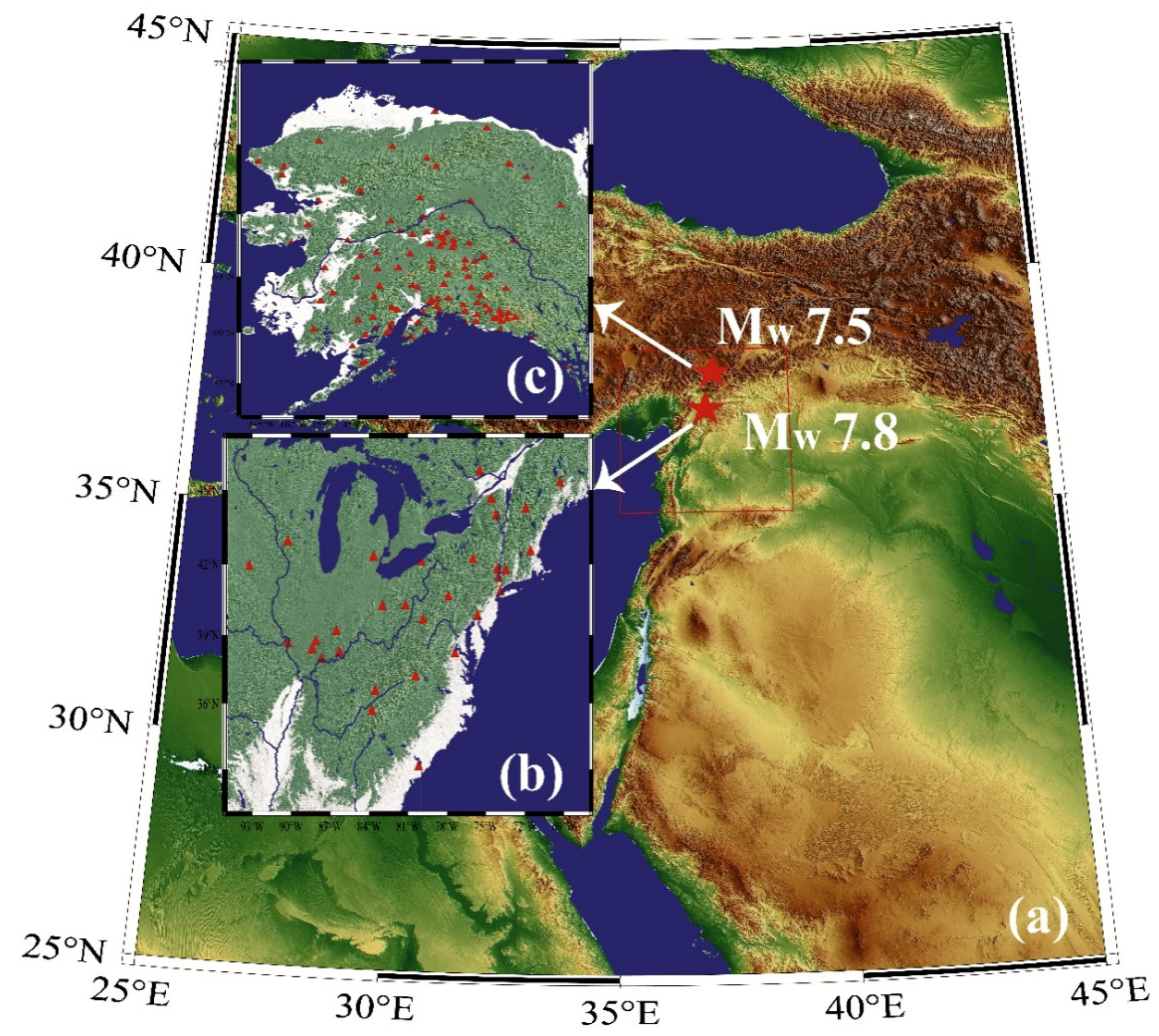
2.1. Geology and Seismic Significance of the Area

The collision of the African and Arabian plates on the south and south-east side of the Anatolian plate form a triple junction [49,50]. The left lateral EAFZ is formed due to break of slabs as the Arabian plate moves northward with overthrust on the Anatolian plate and exerts anti-clockwise rotation to the Anatolian plate [49,51,52,53,54]. The EAFZ exhibits a slip rate of 10 ± 1 mm−1 [55]. The EAFZ is restricted by the Karliova region on the northeast and by the Kahramanmaras region on the southwest, whereas its total length is 550 km [5,16,56,57,58,59,60]. This plate collision has increased the seismicity in the EAFZ (Figure 2). The north–south rending of the Dead Sea Fault Zone (DSFZ), with an estimated length of 1000 km, is also a contributor to the seismicity in the EAFZ [56]. The south end of the DSFZ lies in the Red Sea and, most importantly, its north end merges with the EAFZ at a triple junction point near the Kahramanmaras region [52,56]. On the south side, the Cyprus trench exists due to the compression of the African plate on the Anatolian plate [49,61]. Historical seismicity indicates that the EAFZ was activated through four significant earthquakes of M = 6.9 in 1114, M w = 7.0 in 1795, M w = 7.2 in 1872 and M w = 7.1 in 1893 [52,57]. The Kahramanmaras and Elbistan earthquakes are the most important seismic events occurred along the EAFZ since 1939, when the catastrophic M w = 7.8 Erzincan earthquake happened.

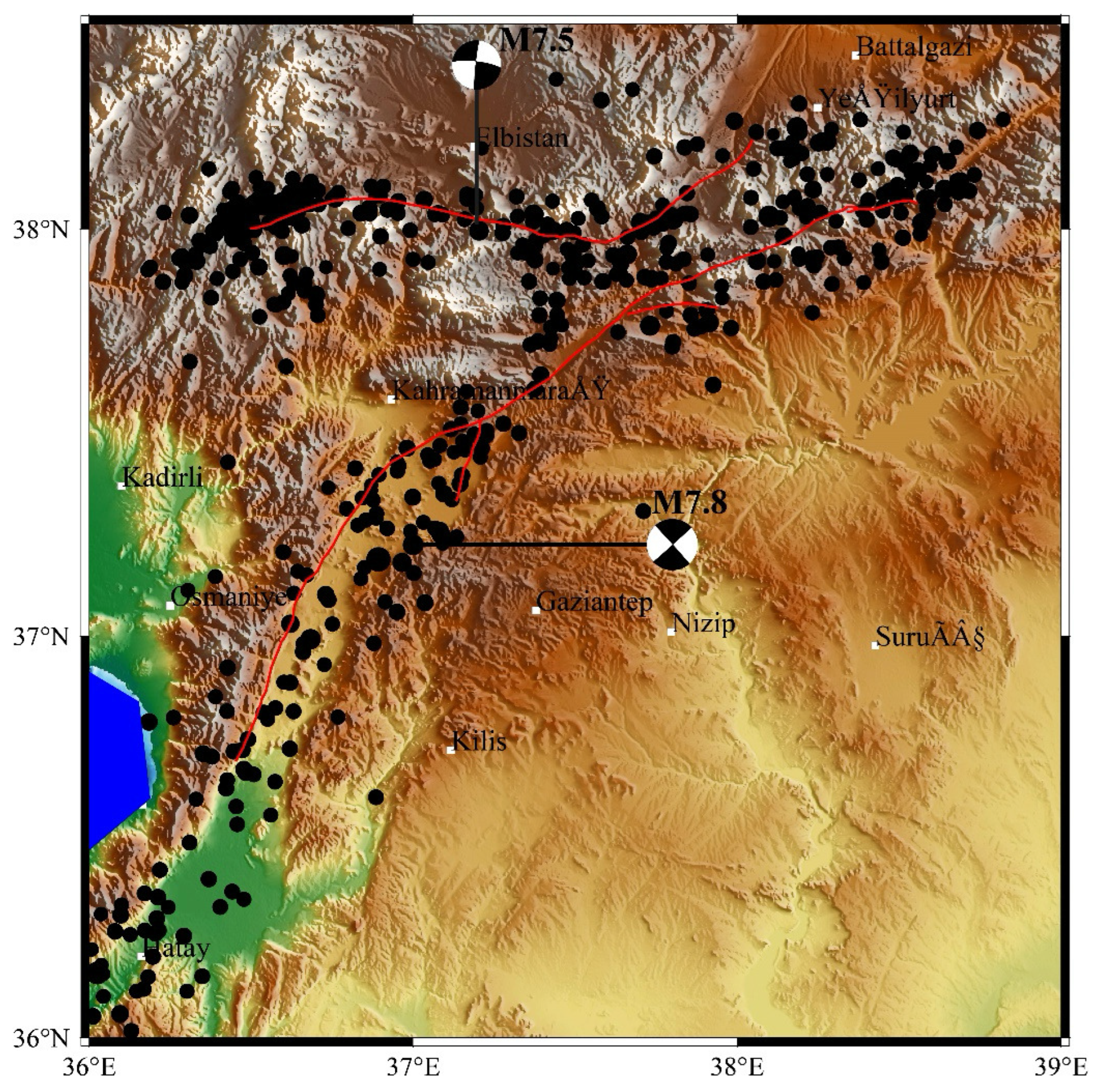
2.2. Studied Earthquakes and Their Importance

On 6 February 2023, two devastating earthquakes struck south-east Turkey near the north-west Syrian border. The first earthquake (Pazarcık) occurred 45 km west of Gaziantep at 1:17:32 (UTC), with a shallow strike-slip faulting at a depth of approximately 8.6 km and a moment magnitude M w = 7.8 [62]. The second earthquake (Elbistan) occurred 66 km north-east of the Kahramanmaraş city centre 9 h later [62,63]. The two earthquakes caused more slip than expected, indicating that they were potentially part of a supercycle, in which the occurrence probability of a large earthquake is determined by accumulated strain rather than time since the last large earthquake [64]. These earthquakes imposed damages in several cities and villages in eleven (11) provinces, including Kahramanmaras Hatay, Adıyaman, Malatya, Adana, and Gaziantep. More than 40,000 buildings collapsed and over 200,000 buildings were affected or heavily damaged in the affected region [63]. These devastating earthquakes caused over 60,000 deaths and 115,000 injuries in south-central Turkey and northwestern Syria [63]. Over about 50,000 aftershocks were detected in the nine months [64]. These detrimental effects indicate clearly how important these earthquakes were on both the natural and anthropogenic environment showing simultaneously their significance in terms of intensity scale both in the vicinity to the earthquakes’ epicentres and away from these [65,66,67]. According to the well-accepted environmental seismic intensity scale of 2007 [66], the co-seismic effects are separated with regard to their diagnostic efficiency into primary and secondary, the former being considered the surface faulting and tectonic and uplift/subsidence and the latter ones comprise the landslides, ground cracks, liquefactions, displaced boulders, tsunami and the hydrological anomalies. As previously mentioned, the Kahramanmaras earthquake is considered to be the mainshock event and the Elbistan earthquake is considered to be the second-largest aftershock. This is based on the fact that the initial mainshock M w = 7.8 rupture at Pazarcık propagated unilaterally on the northernmost part of the DFSZ before transferring to the EAFZ at the Maraş triple junction, causing (according to the event distribution), a shift to the Çardak fault’s positive Coulomb stress, which in turn created dense clusters at both ends of the fault [64]; this origin determines Elbistan’s earthquake to be the second-largest mainshock [64].

2.3. Beamforming Technique

As a backprojection technique, beamforming backprojects the characteristics of the seismic waves in order to estimate the properties of the rupture [68]. Beamforming is robust at visualising the rupture’s propagation: Through the analysis of the Pn phases of the body waves, it simultaneously overcomes limitations due to the high-frequency content of the source’s radiation—both in direction and location—as well as those due to the extent of the rupture. With this technique, the seismic phase timing and the arrival’s azimuth are estimated from the seismic sub-events of the radiating source [69]. In this way, the wave propagation’s pattern and delay are determined, although at a low resolution. Beamfoming additionally calculates the autoproduct phase difference of seismograms from multiple stations even if these exhibit time reversal [45]. By utilising the distinct P waves of coherent signals, beamforming manages to delineate the propagation of the rupture efficiently and with competitive computation performance. It has the ability to extract even weak P wave direct signals from data. Beamforming has an acceptable signal-to-noise ratio with a resolution defined only by the geometry array [37,38,39,40]. However, this latter fact limits its potential since it fails to address the swimming artefacts that cause the energy to burst forwards from the geometric array due to the high frequency content of the large seismic energy released by the sub-events occurring at the earthquake’s hypocentre and the sequential trade-off between rupture time and location [21,45]. Beamforming is applied in the time domain [24,34,45,70]. Beamforming is performed over a sliding window against the stacked energy for each point of rupture [71]. To best estimate the source’s amplitude, linear stacking is applied to beamforming data prior to processing [25,72]. The beamforming steps are described in Ishii et al. [68].
Regarding earthquake-related signals, beamforming was employed with success in the cases of the 2004 M w = 9.2 Sumatra Andaman, Indonesia, earthquake [30,42,43]; the 2008 M w = 7.2 Wenchuan, China, earthquake [73]; the 2005 M w = 7.6 Kashmir, Pakistan, earthquake [74]; the 2010 M w = 8.8 Chile earthquake [37,75]; the 2011 M w = 9.0 Tohoku, Japan, earthquake [76,77,78,79,80,81,82,83]; the 2012 M w = 8.6 Sumatra, Indonesia, offshore earthquake [44,84,85,86]; data from the Helsinki Area, Southern Finland, [87,88]; Salt Lake city, USA [89]; the Gorda plate interface [90]; the Tongzhou, subcenter of Beijing, China [91]; the San Juan, Argentina, earthquake [92]; the aftershocks on the planar rupture surface of the deep-focus M w 7.9 Bonin islands earthquake; long monochromatic earthquake signals [93]; earthquake-related infrasound signals [94,95]; and tsunamigenic earthquakes [96]. Beamforming has successfully outlined earthquake-related rupture length with a maximum of 1300 km (for major earthquakes) and a rupture extent not exceeding 100 s [97].

2.4. Music Backprojection Technique

MUSIC backprojection is a spectral estimation technique based on the covariance matrix of an earthquake-related signal. It is a frequency–wavenumber analysis method for filtered waveforms studied via sliding windows. MUSIC backprojection is hence a technique in the frequency domain of the seismic signal. In the MUSIC backprojection technique, a pseudo-spectrum frequency identifies the arrival’s direction from the hypocentre’s source with maximum spectrum power [29]. The wave field is converted into plane waves with the seismic covariance matrix eigenvector function. Taking the hypocentre as a reference, sub-events are generated by the phase shifting of the plane waves. With the eigenvalue decomposition, a fine-resolution image is produced [69]. In this way, it manages to minimise the variance of the frequency spectrum of wavenumbers and, consequently, the uncertainty of the seismic phase’s arrival time [29]. The direct P-wave’s arrival from the filtered waveform is then aligned and hypothesised to originate from in the hypocenter’s source. Since P-waves have specific directions and velocities through the MUSIC backprojection method decomposition, the noise, which exhibits low amplitudes of eigenvalues, is extracted from the signal, which exhibits high amplitudes of eigenvalues. In this way, the MUSIC backprojection technique manages to estimate the steering vector of the source’s location and the subspace of the noise in an orthogonal frequency vector space [29]. Through this process, however, the information capacity of raw signal’s amplitude decreases and, as a result, the cross-spectrum is estimated within a narrow frequency band. Thereafter, the covariance matrix of the largest eigenvalue is decomposed with an eigenvector into a subspace signal and its complement into noise subspace [84]. In this way, a subspace-spanned signal is defined. During processing with the MUSIC backprojection technique, the arrivals of the direct P waves are aligned via multiple channel cross-correlation.
The MUSIC backprojection technique effectively estimates the arrival direction of long and stationary signals [29]. Moreover, the MUSIC backprojection technique addresses the swimming effect which is a major drawback of all other array techniques. The reader should note here that the swimming effect causes the energy to burst in front of the array due to the high frequencies. This is because large seismic energy is released in the high frequencies due to many microcracks self-organising and forming a large cracked region within a sub-event along an earthquake’s ray path [84]. The MUSIC backprojection technique offers good resolution for large earthquakes and is capable in distinguishing nearby sources [28]. This because it adds a reference station which acts as a window reference for stacking during processing of array data [24,25,69]. Simultaneously, the imaging results of the MUSIC backprojection technique are not affected by the reference statio; however, this is at the expense of computational resources. The MUSIC backprojection technique resolves the rupture’s process spatio-temporally because an earthquake cause multiple faults and of dissimilar focal mechanisms [33]. Note that the conventional backprojection methods cannot easily resolve nearby sources and in this way, the MUSIC backprojection technique is advantageous [74]. However, the most significant gain of the MUSIC backprojection technique is the migration of the swimming effect which is a major artefact of all array techniques [69]. Moreover, the MUSIC backprojection technique effectively estimates the arrival direction of long and stationary signals [29]. In addition, the MUSIC backprojection technique resolves the rupture’s image well, much better than the other array techniques [74].
MUSIC backprojection has also been applied to earthquake-related signals [29,98,99]. The 2013 M w = 8.3 largest deep earthquake in the Sea of Okhotsk off the southwest coast of the Kamchatka-Kurile slab Peninsula in the Russian far east and its sequence have been studied with MUSIC backprojection [29]. Volcanic tremor signals and the earthquakes occurred during the 2014–2015 Holuhraun eruption in Iceland were also investigated with the MUSIC backprojection technique. Fault rupture imaging has been implemented with the MUSIC backprojection technique [98]. The 2018–2022 Hualien earthquake sequence, Taiwan has been investigated with the MUSIC backprojection technique [29]. The MUSIC technique has been applied with success to the 2005 M w = 7.6 Kasmir earthquake, Pakistan [74]. The 2018 M w = 7.5 Palu earthquake-tsunami in the interior of the Molucca sea, Indonesia has been investigated with MUSIC backprojection [22]. The MUSIC technique has been used in the 2016 M w = 6.4 Meinong, Taiwan earthquake has been studied [100]. MUSIC backprojection has been applied to 56 earthquakes from 2010 to 2022 with M W ≥ 7.5 and depth less than 200 km [101]. The 2021 M w = 7.1 Fukushima earthquake, Japan has also been studied with the MUSIC technique [102].

2.5. Data and Methodology

As mentioned in Section 1, the array of seismic data in this paper is acquired from 32 broadband stations of the USArray network of the US and from 104 broadband stations installed in Canada. Both networks are oriented approximately in parallel to the dominant direction of the EAFZ and therefore the spatial resolution of the acquired data is better along the ruptured fault. Broadband seismic station arrays are derived both for the main M w = 7.8 Kahramanmaras earthquake and the M w = 7.5 Elbistan second-largest mainshock. First, the seismograms of the direct P-waveforms with clear reference [30] are aligned through a bandpass frequency filter applied at time t = 0 s (arrival time). This is performed by computing the cross-correlation of the first Pn arrivals with 10 s windows [95], taking into account the hypocenter’s latitude, longitude, and depth. Through this approach, the uncertainties for the structure of velocity are minimized. Note that these uncertainties may cause errors in estimation of the travel time [30]. Importantly, the seismogram alignment eliminates the delay due to localised side effects [83]. As a result, the energy released from the source is extracted in a compressed form in the frequency domain [83].
Both for the 2023 M w = 7.8 Kahramanmaras earthquake and the M w = 7.5 Elbistan second largest mainshock, the seismograms exhibit a dominant frequency at 0.6 Hz. To cover this frequency, a range of filters is applied between 0.5 Hz and 1 Hz and the P-waveform is aligned using the cross correlation with each earthquake’s epicentre as a reference [9]. The source region is then segmented into small grids. The filtered teleseismic P-waveform is thereafter backprojected to the source. The travel time variation due to the earth’s structure between the source and the receiver is taken into account during backprojection. The velocity of the rupture’s front is performed with the 1-D reference model IASP91 [48], both for the Kahramanmaras main event and the Elbistan second largest mainshock. Note, that backprojection dominates also at 0.6 Hz and therefore, the 0.6 Hz filter resembles the rupture’s shear velocity [103]. Since the resolution of the array of events depends on the waveform’s coherence–incoherence and its interference., the filter at 0.6 Hz addresses the time-frequency trade-off and the coherency of the array data and this should be emphasised. Significantly, both earthquakes are taken as an array of sub-events of the event series along the rupture that radiates energy at high frequencies [104]. The array network processing and the image generation with the MUSIC backprojection technique enhances temporal evolution. For better resolution with the MUSIC backprojection technique the calibration of slowness is carried out [69]. Importantly, cross-spectrum narrow-band estimates are also employed in the MUSIC backprojection technique.

3. Results and Discussion

The rupture of the Kahramanmaras and Elbistan earthquakes started with the occurrence of the Kahramanmaras earthquake on 6 of February 2023 and thereafter propagated and radiated energy along the whole of the activated region of the fault zone [105]. Beamforming identifies three segments for the rupture of the Kahramanmaras earthquake (Figure 3 as there is a concentration of red-orange yellow points between 34.5° and 37.5° longitude and 37.0° and 37.5° latitude along the downward fault (red) line (segment 1), a second concentration of dark blue lines between 37.0° and 37.5° longitude and around 37.5° latitude (segment 2) and the remaining series of mainly cyan points approximately above 37.0° longitude and above 37.5° latitude (segment 3). Interestingly, segment 2 points are near the Kahramanmaras earthquake’s epicentre. As can be observed in Figure 3a, beamforming is not successful in resolving the extent and the pattern of the rupture because it gives puzzled information regarding both the direction and the limits of the rupture. Indeed, in both figures, the majority of the data points are away from the activated fault segment (red lines). This may be attributed to the swimming effect and to potential deviations between the actual velocities of the sub-surface and the ones according by the IASP91 model. On the other hand, beamforming successfully distinguishes the rupture’s extent from the fault’s geometry Figure 3. Indeed, the black lines which delimit rupture’s extent are well away from the red ones for of both sub-figures of Figure 3a, i.e., this is valid for both the Kahramanmaras earthquake and the Elbistan second-largest mainshock. This can be explained by the fact that the high-frequency coherent P-body waves are related both to the earthquake’s triggering and its extent [75,106,107].
As with beamforming, MUSIC backprojection identifies three segments for the rupture of the Kahramanmaras earthquake (Figure 4a). The first segment (segment 1) is observed for the concentration of red and orange and some green points between 36.5° and 37.0° longitude and around 37.0° latitude. The second segment (segment 2) is for the concentration of dark blue points between 37.0° and 37.5° longitude and around 37.5° latitude. This segment is also near the Kahramanmaras earthquake’s epicentre and this should be emphasised. It is significant and should be pointed out that both beamforming and MUSIC backprojection technique coincide in the longitude–latitude and intensity findings from the dark blue points around the earthquake’s epicentre. The third segment (segment 3) is for the concentration of light blue–cyan points approximately above 37.0° longitude and above 37.5° latitude, importantly, at the same longitude–latitude ranges as the ones of segment 3 points from the beamforming technique. However, in both Figure 3a (beamforming Kahramanmaras earthquake’s results) and Figure 4a (MUSIC backprojection’s Kahramanmaras earthquake’s results) there are points that are away from the downward fault (red) line, indicating rupture’s spatial discrepancies for both techniques. This is more pronounced for the results of the backprojection’s technique. As has been explained already in several parts of the text above, MUSIC backprojection is advantageous for the investigation of the rupture of earthquakes [100].
The Elbistan second-largest mainshock evokes in the upward fault three more segments in the outcomes from the application of MUSIC backprojection Figure 4b. The first segment (segment 1) is found between 36.5° and 37.0° longitude and around 38.0° latitude where red and orange points concentrate. The second segment (segment 2) is observed as a concentration of dark blue points around 37.5° longitude and 38.0° latitude. This segment is also near the Elbistan aftershock’s epicentre.The third segment (segment 3) is found as a concentration of light blue-cyan and green points around 38.0° longitude and latitude. Only six points deviate from the upward fault (red) line, whereas two point are in the downward fault line. Beamforming rather fails to discriminate these segments. Only some dark blue, cyan, and green points are within the upward fault line. However, there is a discrete concentration of red-orange points between 37.0° and 38.5° longitude and between 38.5° and 39.0° longitude. In this sense, beamforming seems to discriminate two segments. Both backprojection techniques identify discrete intensity segments. Five (5) total segments are found by beamfoming while MUSIC backprojection technique identifies six (6) segments. This is in line with the international literature. Indeed, as already mentioned, backprojection suffers from artefacts due to swimming effects whereas MUSIC backprojection is not sensitive to these [1,24,29,45,69,95,100]. As already mentioned, the swimming effects are a significant factor of point deviations between these two techniques because they cause the seismic energy to burst in front of the array of stations’ data due to the high frequencies contribution [17,22,24,29]. Another mentioned reason is potentially the deviation between the actual velocities of the sub-surface and those calculated by the IASP91 model [2,6,43,59,73,101]. As both backprojection techniques indicate, some intensity points are scattered and away from the points’ mainstream. This is more or less expected since the evolution of both Kahramanmaras and Elbistan earthquakes were complex [55,58,60,108] and as a result the rupture’s evolution is hard to predict fully. Moreover, the progress of earthquakes follow fractal patterns of self-organised criticality [109] and as a result the rupture’s progress can be strongly biased by these physical pathways adding more deviation to the results’ data. On the other hand, both beamforming and MUSIC backprojection techniques coincide in the longitude–latitude and intensity findings from the dark blue points around the earthquakes and especially near both epicentres.This is also significant and should be emphasised. For both earthquakes, the beamforming and MUSIC backprojection techniques indicate a main concentration points being along the direction of the dissipation of the energy.
The rupture velocities of the segments of both events can be calculated by estimating the slip rate through the corresponding slip model of each ruptured patch [103]. Through this approach, the velocities of the rupture are divided in six (6) velocity segments (Figure 5). Three velocity segments of the downward fault (segments 1, 2a, 2b, and 3) are due to M w = 7.8 Kahramanmaras earthquake and the remaining segments (segments 4 and 5) are in the upward fault line and caused by the M w = 7.5 Elbistan second-largest mainshock. Since the M w = 7.8 Kahramanmaras earthquake was generated at the splay of the EAFZ 16 km away from the main fault, the rupture initiating from the earthquake’s epicentre covered the 16 km distance in 6 s. That occurred in the first velocity segment and moved towards the main EAFZ. In the second velocity segment, the rupture exhibited a bidirectional pattern on the northeast and southwest sides but yields different velocities, possibly due to lithological differences. Therefore, the second velocity segment is divided into two sub-segments, namely segment 2a (northeast side) and segment 2b (southwest side). Segment 2a covered the 108 km distance of along the main fault along the northeast direction in 35 s with an average velocity of 3.1 km/s. Simultaneously, the rupture propagated in the southwest side namely, segment 2b covered the distance of 35 km in 10.5 s with an average velocity of 3.4 km/s. After covering the distance of 35 km, the 2b segment’s rupture was momentarily blocked. For segment 2b, the average velocity is near to super-shear velocity, i.e., it is a sub-shear velocity. After 41 s, the third segment initiated along the south side of the main fault. The direction of segment 3 is southeast with a dominant direction southwards. This process continued for the next 42 s and covered the distance of 140 km before the rupture’s arrest. Segment 3 has an average velocity of 3.3 km/s as shown in Figure 5. Therefore, these segment rupture seizures may be due to the transition zone of brittle-ductile subsurface material along the fault. The Elbistan major second-largest mainshock was a left-lateral strike-slip fault [59,60,108] that occurred 9 h and 7 min after the main event and propagated in both directions from the epicentre. The first phase of this second-largest mainshock corresponds to segment 4. Its rupture propagated along the northeast direction with an average velocity of 3.21 km/s. The duration of this segment was 28 s and covered 90 km distance. The rupture re-initiated from the epicentre in segment 5 along the southwest direction. It attained an average velocity of 3.4 km/s which approaches a super-shear velocity (Figure 5). This may be due to its strike-slip nature [71]. The total distance covered in this segment is 60 km with a duration of 17.5 s before the rupture stopped. Hence, the total rupture’s velocity is 3.2 km/s. Table 1 presents the information of all the segments.
From the above data, it becomes evident that both earthquake events attain on average sub- and super-shear velocity. It is interesting that sub- and super-shear velocity have been reported for the same earthquake doublet also by a recent publication [59]. Super-shear velocity was observed in the 2002 Denali fault earthquake [110]; in the 2010 Qinghai, China, earthquake [111]; in the 2013 Craig, Alaska, M w = 7.5 earthquake [112]; in the M w = 6.7 aftershock of the 2013 Sea of Okhotsk earthquake [113]; in several short-period earthquakes [101]; in laboratory earthquakes along inhomogeneous faults [114]; and in several oceanic and continental earthquakes [70]. It should be mentioned here that both earthquakes have bilateral rupture’s propagation but, as mentioned above, with different velocities and segments. According to the findings, the rupture nucleates along the strike. A possible explanation is that the nucleation propagation of the rupture initiates when the strength exceeds the strength of the fault and this happens when the strength of the rupture exceeds the friction of the fault, which is the barrier for the propagation of the rupture [115]. This means, in turn, that the ruptured segments of the fault along the main event, may be an indication that the subsurface lithology transit between brittle and ductile materials. All these occur possibly at the hypocentres of both earthquakes. The rupture’s segments are captured in the frequency range between 0.5 Hz and 1.0 Hz indicating a frequency range including, interestingly, the dominant P-wave frequency of 0.6 Hz. At the tip of each segment, the extent of the propagating rupture more or less runs into the surrounding lithology but encounters obstacles because of increased strength at the boundary of the sub surface and below. This, in turn, causes the first rupture to stagnate and then stop due to the propagation’s phase. Both stress and friction of the fault’s lane impose damages along the affected area depending on the rupture’s velocity and its extent both relating to the properties of fault zone [105]. Estimating the rupture’s segmentation, direction, velocity and extent through phase-coherent direct P-waves is a significant approach to delineating earthquake-related parameters. Although earthquakes are still hard to forecast [109], the scientific efforts to delineate the associated rupture is of great importance especially for catastrophic earthquakes as the seismic doublet of Turkey, 2023.

4. Conclusions

In this paper, backprojection source imaging techniques are utilised for body waves recorded by seismic arrays at regional scale distances via P-direct waves. The employed methods are conventional beamforming and the MUSIC backprojection. In particular, the MUSIC backprojection method is applied with multi-taper cross-spectral estimation and achieves sharp source imaging. Through these techniques, key rupture aspects are extracted, such as the location and evolution of the high frequency radiation sources of the rupture’s process. The dominant P-wave frequency is 0.6 Hz, whereas the rupture’s segments range between 0.5 Hz and 1.0 Hz. Three (3) rupture’s segments are identified for the Kahramanmaras earthquake between 34.5–37.5° longitude and 37.0–37.5° latitude and another three (3) for the Elbistan second-largest aftershock between 36.5–38.0° longitude and around 38.5° latitude. Differentiations exist between beamforming and MUSIC backprojection techniques, the former being sensitive to swimming artefacts. The MUSIC backprojection technique resolves the rupture’s segments and quantifies the rupture behaviour of both events. This is because the sliding concept of the reference window that is applied in MUSIC backprojection at low frequencies enables the mitigation of the swimming artefact on the time-shift stack, which is a result of the non-stationarity of the recorded signals. The beamforming technique is not as efficient at resolving rupture process in any case. At the end tip of the rupture’s extent, the originated high-frequency radiation arrests. As a result, the end tip of each segment is delimited along with the extent of the rupture. The results of the rupture velocities indicate that there are phases of approximately super-shear rupture velocity for both the main Kahramanmaras earthquake and the Elbistan second-largest mainshock. Rupture velocities range between 3.1 km/s and 3.4 km/s. Five (5) velocity segments are identified, three (3) for the Kahramanmaras and two (2) for the Elbistan earthquake. Beamforming is very efficient at identifying the velocity segments. In contrast, the MUSIC backprojection technique efficiently resolved the velocity segments and quantified the rupture behaviour of both events. This is because the sliding concept of the reference window that is applied in MUSIC backprojection at low frequencies enabling the mitigation of the swimming artefact on the time-shift stack, which is a result of the non-stationarity of the recorded signals. The MUSIC backprojection method’s results revealed the rupture’s and velocity’s segments and their process for both the 2023 M w = 7.8, Kahramanmaras earthquake and the M w = 7.5 Elbistan second-largest mainshock.The three velocity segments identified of the main event cover a total distance of 299 km in 185 s. The two segments of the Elbistan earthquake cover a total distance of 150 km in 46 s. Comparing beamforming and MUSIC backprojection techniques outputs, the results from MUSIC backprojection techniques are more reliable for delineating the rupture’s processes of both earthquakes under investigation.

5. Evaluation and Limitations

The approach followed in this paper focused on a very important earthquake doublet that occurred recently (2023) in Turkey. These earthquakes imposed significant damages and the investigation of the rupture of these earthquakes makes this a paper of interest as a result. Due to the significance of these earthquakes, several papers were published. A selected set of these is presented in this paper. The investigation included two well-accepted techniques with very recent publications on the subject. Both facts add value to this research. The employed techniques have been and are used by investigators for the study of earthquakes’ associated rupture and the spatio-temporal characteristics of this. According to presented literature data, numerous medium and large earthquakes have been studied with beamforming and, especially, MUSIC backprojection. The techniques estimated the rupture’s spatial characteristics but not the temporal ones. This is a limitation. Rupture and velocity segments were identified and quantified. On the other hand, the 1D velocity model used is from 1991; despite that, it is still in use. The use of 3D velocity models will be a future approach, but their absence in this paper is another limitation. This paper basically concluded that both events are associated with sub- and super-shear velocity. This was found by other publications, especially for the same earthquake doublet. This is a positive contribution. In general, this paper outlined and utilised mainly recent references and showed that there exists scientific interest in this subject. The application of these techniques to more earthquakes is needed to establish its generality and usability.

Author Contributions

Conceptualization, D.N. and M.S.; methodology, D.N., A.A., D.C., G.P. (Georgios Prezerakos), M.P. and J.S.; software, G.P. (Georgios Priniotakis), D.C., M.P., A.A., M.S. and J.S.; formal analysis, D.N., G.P. (Georgios Prezerakos), M.P., D.C., P.Y., F.J., M.R. and G.P. (Georgios Priniotakis); investigation, D.N., D.C., P.Y., G.P. (Georgios Priniotakis), G.P. (Georgios Prezerakos), M.R., M.P., J.S. and M.R.; resources, M.S., A.A., J.S., M.A.S., M.R. and F.J.; data curation, D.N., G.P. (Georgios Prezerakos), M.P., P.Y., G.P. (Georgios Priniotakis), M.S. and A.A.; writing—original draft preparation, D.N., M.S., A.A., F.J., J.S. and M.R.; writing—review and editing, D.N., G.P. (Georgios Prezerakos), G.P. (Georgios Priniotakis), M.P., P.Y., D.C., M.S., M.R. and A.A.; visualization, M.S.; supervision, D.N. and M.R.; project administration, D.N. and A.A. All authors have read and agreed to the published version of the manuscript.

Funding

This research received no external funding.

Data Availability Statement

3rd Party Data. The data can be downloaded from “https://ds.iris.edu/ds/nodes/dmc/forms/sac/ (accessed on 9 April 2025)” with the permission of NSF SAGE “https://ds.iris.edu/ds/ (accessed on 9 April 2025)”.

Conflicts of Interest

The authors declare no conflicts of interest.

References

  1. Cao, B.; Ge, Z. Cascading multi-segment rupture process of the 2023 Turkish earthquake doublet on a complex fault system revealed by teleseismic P wave back projection method. Earthq. Sci. 2024, 37, 158–173. [Google Scholar] [CrossRef]
  2. Hayes, G.P. The finite, kinematic rupture properties of great-sized earthquakes since 1990. Earth Planet. Sci. Lett. 2017, 468, 94–100. [Google Scholar] [CrossRef]
  3. Mendoza, C.; Hartzell, S.; Ramirez-Guzman, L.; Martinez-Lopez, R. Prediction of Regional Broadband Strong Ground Motions Using a Teleseismic Source Model of the 18 April 2014 Mw 7.3 Papanoa, Mexico, Earthquake. Bull. Seismol. Soc. Am. 2024, 114, 2524–2545. [Google Scholar] [CrossRef]
  4. Xu, C.; Zhang, Y.; Hua, S.; Zhang, X.; Xu, L.; Chen, Y.; Taymaz, T. Rapid source inversions of the 2023 SE Türkiye earthquakes with teleseismic and strong-motion data. Earthq. Sci. 2023, 36, 316–327. [Google Scholar] [CrossRef]
  5. Taymaz, T.; Ganas, A.; Yolsal-Çevikbilen, S.; Vera, F.; Eken, T.; Erman, C.; Keleş, D.; Kapetanidis, V.; Valkaniotis, S.; Karasante, I.; et al. Source mechanism and rupture process of the 24 January 2020 Mw 6.7 Doğanyol–Sivrice earthquake obtained from seismological waveform analysis and space geodetic observations on the East Anatolian Fault Zone (Turkey). Tectonophysics 2021, 804, 228745. [Google Scholar] [CrossRef]
  6. Goldberg, D.E.; Koch, P.; Melgar, D.; Riquelme, S.; Yeck, W.L. Beyond the Teleseism: Introducing Regional Seismic and Geodetic Data into Routine USGS Finite-Fault Modeling. Seismol. Res. Lett. 2022, 93, 3308–3323. [Google Scholar] [CrossRef]
  7. Chelidze, T.; Matcharashvili, T.; Varamashvili, N.; Mepharidze, E.; Tephnadze, D.; Chelidze, Z. 9—Complexity and Synchronization Analysis in Natural and Dynamically Forced Stick–Slip: A Review. In Complexity of Seismic Time Series; Chelidze, T., Vallianatos, F., Telesca, L., Eds.; Elsevier: Amsterdam, The Netherlands, 2018; pp. 275–320. [Google Scholar] [CrossRef]
  8. Ringler, A.T.; Anthony, R.E.; Aster, R.C.; Ammon, C.J.; Arrowsmith, S.; Benz, H.; Ebeling, C.; Frassetto, A.; Kim, W.Y.; Koelemeijer, P.; et al. Achievements and Prospects of Global Broadband Seismographic Networks After 30 Years of Continuous Geophysical Observations. Rev. Geophys. 2022, 60, e2021RG000749. [Google Scholar] [CrossRef]
  9. Kato, S.; Nishida, K. Extraction of Mantle Discontinuities From Teleseismic Body-Wave Microseisms. Geophys. Res. Lett. 2023, 50, e2023GL105017. [Google Scholar] [CrossRef]
  10. Deng, Y.; Byrnes, J.S.; Bezada, M. New Insights Into the Heterogeneity of the Lithosphere-Asthenosphere System Beneath South China From Teleseismic Body-Wave Attenuation. Geophys. Res. Lett. 2021, 48, e2020GL091654. [Google Scholar] [CrossRef]
  11. Shrivastava, A.; Liu, K.H.; Gao, S.S. Teleseismic P-Wave Attenuation Beneath the Southeastern United States. Geochem. Geophys. Geosyst. 2021, 22, e2021GC009715. [Google Scholar] [CrossRef]
  12. Li, L.; Boué, P.; Campillo, M. Observation and explanation of spurious seismic signals emerging in teleseismic noise correlations. Solid Earth 2020, 11, 173–184. [Google Scholar] [CrossRef]
  13. Li, B.; Wu, B.; Bao, H.; Oglesby, D.D.; Ghosh, A.; Gabriel, A.A.; Meng, L.; Chu, R. Rupture Heterogeneity and Directivity Effects in Back-Projection Analysis. J. Geophys. Res. Solid Earth 2022, 127, e2021JB022663. [Google Scholar] [CrossRef]
  14. Song, X. Seismic Array Imaging of Teleseismic Body Wsves from Finite-Frequency Tomography to Full Waveform Invesrions: With Applications to South-Central Alska Subduction Zone. Ph.D. Thesis, Graduate Department of Physics, University of Toronto, Toronto, ON, Canada, 2019. [Google Scholar]
  15. Yin, J.; Denolle, M.A. Relating teleseismic backprojection images to earthquake kinematics. Geophys. J. Int. 2019, 217, 729–747. [Google Scholar] [CrossRef]
  16. Zhang, Y.; Tang, X.; Liu, D.; Taymaz, T.; Eken, T.; Guo, R.; Zheng, Y.; Wang, J.; Sun, H. Geometric controls on cascading rupture of the 2023 Kahramanmaraşearthquake doublet. Nat. Geosci. 2023, 16, 1054–1060. [Google Scholar] [CrossRef]
  17. Du, H. Estimating rupture front of large earthquakes using a novel multi-array back-projection method. Front. Earth Sci. 2021, 9, 680163. [Google Scholar] [CrossRef]
  18. Steinberg, A.; Sudhaus, H.; Krüger, F. Using teleseismic backprojection and InSAR to obtain segmentation information for large earthquakes: A case study of the 2016 Mw 6.6 Muji earthquake. Geophys. J. Int. 2022, 232, 1482–1502. [Google Scholar] [CrossRef]
  19. Meng, L.; Zhang, A.; Yagi, Y. Improving back projection imaging with a novel physics-based aftershock calibration approach: A case study of the 2015 Gorkha earthquake. Geophys. Res. Lett. 2016, 43, 628–636. [Google Scholar] [CrossRef]
  20. Zhang, H.; Koper, K.D.; Pankow, K.; Ge, Z. Imaging the 2016 Mw 7.8 Kaikoura, New Zealand, earthquake with teleseismic P waves: A cascading rupture across multiple faults. Geophys. Res. Lett. 2017, 44, 4790–4798. [Google Scholar] [CrossRef]
  21. Meng, L.; Bao, H.; Huang, H.; Zhang, A.; Bloore, A.; Liu, Z. Double pincer movement: Encircling rupture splitting during the 2015 Mw 8.3 Illapel earthquake. Earth Planet. Sci. Lett. 2018, 495, 164–173. [Google Scholar] [CrossRef]
  22. Fahmi, M.N.; Realita, A.; Risanti, H.; Prastowo, T.; Madlazim. Back-projection results for the Mw 7.5, 28 September 2018 Palu earthquake-tsunami. J. Phys. Conf. Ser. 2022, 2377, 012032. [Google Scholar] [CrossRef]
  23. Xie, Y.; Meng, L.; Zhou, T.; Xu, L.; Bao, H.; Chu, R. The 2021 Mw 7.3 East Cape Earthquake: Triggered Rupture in Complex Faulting Revealed by Multi-Array Back-Projections. Geophys. Res. Lett. 2022, 49, e2022GL099643. [Google Scholar] [CrossRef]
  24. Claudino, C.; Lupinacci, W.M. The spectral stacking method and its application in seismic data resolution increase. Geophys. Prospect. 2023, 71, 509–517. [Google Scholar] [CrossRef]
  25. Lai, H.; Garnero, E.J. Travel time and waveform measurements of global multibounce seismic waves using virtual station seismogram stacks. Geochem. Geophys. Geosyst. 2020, 21, e2019GC008679. [Google Scholar] [CrossRef]
  26. Wu, H.; Xiao, W.; Ren, H. Automatic time picking for weak seismic phase in the strong noise and interference environment: An hybrid method based on array similarity. Sensors 2022, 22, 9924. [Google Scholar] [CrossRef] [PubMed]
  27. Xie, Y.; Bao, H.; Meng, L. Source Imaging With a Multi-Array Local Back-Projection and Its Application to the 2019 Mw 6.4 and Mw 7.1 Ridgecrest Earthquakes. J. Geophys. Res. Solid Earth 2021, 126, e2020JB021396. [Google Scholar] [CrossRef]
  28. Kiser, E.; Ishii, M. Back-projection imaging of earthquakes. Annu. Rev. Earth Planet. Sci. 2017, 45, 271–299. [Google Scholar] [CrossRef]
  29. Jian, P.R.; Wang, Y. Applying unsupervised machine-learning algorithms and MUSIC back-projection to characterize 2018–2022 Hualien earthquake sequence. Terr. Atmos. Ocean. Sci. 2022, 33, 28. [Google Scholar] [CrossRef]
  30. Ishii, M.; Shearer, P.M.; Houston, H.; Vidale, J.E. Extent, duration and speed of the 2004 Sumatra–Andaman earthquake imaged by the Hi-Net array. Nature 2005, 435, 933–936. [Google Scholar] [CrossRef]
  31. Kiser, E.; Ishii, M. Combining seismic arrays to image the high-frequency characteristics of large earthquakes. Geophys. J. Int. 2012, 188, 1117–1128. [Google Scholar] [CrossRef]
  32. Neo, J.C.; Fan, W.; Huang, Y.; Dowling, D. Frequency-difference backprojection of earthquakes. Geophys. J. Int. 2022, 231, 2173–2185. [Google Scholar] [CrossRef]
  33. Zeng, H.; Wei, S.; Wu, W. Sources of uncertainties and artefacts in back-projection results. Geophys. J. Int. 2019, 220, 876–891. [Google Scholar] [CrossRef]
  34. Tan, F.; Ge, Z.; Kao, H.; Nissen, E. Validation of the 3-D phase-weighted relative back projection technique and its application to the 2016 Mw 7.8 Kaikōura Earthquake. Geophys. J. Int. 2019, 217, 375–388. [Google Scholar] [CrossRef]
  35. Vera, F.; Tilmann, F.; Saul, J.; Evangelidis, C.P. Imaging the 2007 Mw 7.7 Tocopilla earthquake from short-period back-projection. J. S. Am. Earth Sci. 2023, 127, 104399. [Google Scholar] [CrossRef]
  36. Zhang, H.; Ge, Z. Stepover rupture of the 2014 Mw 7.0 Yutian, Xinjiang, Earthquake. Bull. Seismol. Soc. Am. 2017, 107, 581–591. [Google Scholar] [CrossRef]
  37. Liu, Z.; Song, C.; Meng, L.; Ge, Z.; Huang, Q.; Wu, Q. Utilizing a 3D global P-wave tomography model to improve backprojection imaging: A case study of the 2015 Nepal earthquake. Bull. Seismol. Soc. Am. 2017, 107, 2459–2466. [Google Scholar] [CrossRef]
  38. Qin, W.; Yao, H. Characteristics of subevents and three-stage rupture processes of the 2015 Mw 7.8 Gorkha Nepal earthquake from multiple-array back projection. J. Asian Earth Sci. 2017, 133, 72–79. [Google Scholar] [CrossRef]
  39. Yagi, Y.; Okuwaki, R. Integrated seismic source model of the 2015 Gorkha, Nepal, earthquake. Geophys. Res. Lett. 2015, 42, 6229–6235. [Google Scholar] [CrossRef]
  40. Zhang, H.; Van Der Lee, S.; Ge, Z. Multiarray rupture imaging of the devastating 2015 Gorkha, Nepal, earthquake sequence. Geophys. Res. Lett. 2016, 43, 584–591. [Google Scholar] [CrossRef]
  41. Nissen, E.; Elliott, J.; Sloan, R.; Craig, T.; Funning, G.; Hutko, A.; Parsons, B.; Wright, T. Limitations of rupture forecasting exposed by instantaneously triggered earthquake doublet. Nat. Geosci. 2016, 9, 330–336. [Google Scholar] [CrossRef]
  42. Bletery, Q.; Sladen, A.; Jiang, J.; Simons, M. A Bayesian source model for the 2004 great Sumatra-Andaman earthquake. J. Geophys. Res. Solid Earth 2016, 121, 5116–5135. [Google Scholar] [CrossRef]
  43. Fan, W.; Shearer, P.M. Coherent seismic arrivals in the P wave coda of the 2012 Mw 7.2 Sumatra earthquake: Water reverberations or an early aftershock? J. Geophys. Res. Solid Earth 2018, 123, 3147–3159. [Google Scholar] [CrossRef]
  44. Meng, L.; Ampuero, J.P.; Luo, Y.; Wu, W.; Ni, S. Mitigating artifacts in back-projection source imaging with implications for frequency-dependent properties of the Tohoku-Oki earthquake. Earth Planets Space 2012, 64, 1101–1109. [Google Scholar] [CrossRef]
  45. Bowden, D.C.; Sager, K.; Fichtner, A.; Chmiel, M. Connecting beamforming and kernel-based noise source inversion. Geophys. J. Int. 2020, 224, 1607–1620. [Google Scholar] [CrossRef]
  46. Zhang, H.; Vidale, J.E.; Wang, W. Aftershocks on the Planar Rupture Surface of the Deep-Focus Mw 7.9 Bonin Islands Earthquake. Seism. Rec. 2025, 5, 35–43. [Google Scholar] [CrossRef]
  47. Guilbert, J.; Vergoz, J.; Schisselé, E.; Roueff, A.; Cansi, Y. Use of hydroacoustic and seismic arrays to observe rupture propagation and source extent of the Mw = 9.0 Sumatra earthquake. Geophys. Res. Lett. 2005, 32, L15310. [Google Scholar] [CrossRef]
  48. Kennett, B.L.N.; Engdahl, E.R.; Buland, R. Constraints on seismic velocities in the Earth from traveltimes. Geophys. J. Int. 1995, 122, 108–124. [Google Scholar] [CrossRef]
  49. Delph, J.R.; Abgarmi, B.; Ward, K.M.; Beck, S.L.; Özacar, A.A.; Zandt, G.; Sandvol, E.; Türkelli, N.; Kalafat, D. The effects of subduction termination on the continental lithosphere: Linking volcanism, deformation, surface uplift, and slab tearing in central Anatolia. Geosphere 2017, 13, 1788–1805. [Google Scholar] [CrossRef]
  50. Ahadov, B.; Jin, S. Present-day kinematics in the Eastern Mediterranean and Caucasus from dense GPS observations. Phys. Earth Planet. Inter. 2017, 268, 54–64. [Google Scholar] [CrossRef]
  51. Bartol, J.; Govers, R. A single cause for uplift of the Central and Eastern Anatolian plateau? Tectonophysics 2014, 637, 116–136. [Google Scholar] [CrossRef]
  52. Güvercin, S.E.; Karabulut, H.; Konca, A.Ö.; Doğan, U.; Ergintav, S. Active seismotectonics of the East Anatolian fault. Geophys. J. Int. 2022, 230, 50–69. [Google Scholar] [CrossRef]
  53. Mahatsente, R.; Önal, G.; Çemen, I. Lithospheric structure and the isostatic state of Eastern Anatolia: Insight from gravity data modelling. Lithosphere 2018, 10, 279–290. [Google Scholar] [CrossRef]
  54. Schildgen, T.F.; Yıldırım, C.; Cosentino, D.; Strecker, M.R. Linking slab break-off, Hellenic trench retreat, and uplift of the Central and Eastern Anatolian plateaus. Earth-Sci. Rev. 2014, 128, 147–168. [Google Scholar] [CrossRef]
  55. Bayrak, E.; Yılmaz, Ş.; Softa, M.; Türker, T.; Bayrak, Y. Earthquake hazard analysis for East Anatolian fault zone, Turkey. Nat. Hazards 2015, 76, 1063–1077. [Google Scholar] [CrossRef]
  56. Altunel, E.; Kozacı, Ö.; Yıldırım, C.; Sbeinati, R.M.; Meghraoui, M. Potential domino effect of the 2023 Kahramanmaraşearthquake on the centuries-long seismic quiescence of the Dead Sea fault: Inferences from the North Anatolian fault. Sci. Rep. 2024, 14, 15440. [Google Scholar] [CrossRef]
  57. Ambraseys, N. Earthquakes in the Mediterranean and Middle East: A Multidisciplinary Study of Seismicity up to 1900; Cambridge University Press: Cambridge, UK, 2009. [Google Scholar]
  58. Chen, W.; Rao, G.; Kang, D.; Wan, Z.; Wang, D. Early Report of the Source Characteristics, Ground Motions, and Casualty Estimates of the 2023 Mw 7.8 and 7.5 Turkey Earthquakes. J. Earth Sci. 2023, 34, 297–303. [Google Scholar] [CrossRef]
  59. Melgar, D.; Taymaz, T.; Ganas, A.; Crowell, B.W.; Öcalan, T.; Kahraman, M.; Tsironi, V.; Yolsal-Çevikbil, S.; Valkaniotis, S.; Irmak, T.S.; et al. Sub-and super-shear ruptures during the 2023 Mw 7.8 and Mw 7.6 earthquake doublet in SE Türkiye. Seismica 2023, 2, 387. [Google Scholar] [CrossRef]
  60. Melgar, D.; Ganas, A.; Taymaz, T.; Valkaniotis, S.; Crowell, B.W.; Kapetanidis, V.; Tsironi, V.; Yolsal-Çevikbilen, S.; Öcalan, T. Rupture kinematics of 2020 January 24 Mw 6.7 Doğanyol-Sivrice, Turkey earthquake on the East Anatolian Fault Zone imaged by space geodesy. Geophys. J. Int. 2020, 223, 862–874. [Google Scholar] [CrossRef]
  61. Kusky, T.M.; Bozkurt, E.; Meng, J.; Wang, L. Twin earthquakes devastate southeast Türkiye and Syria: First report from the epicenters. J. Earth Sci. 2023, 34, 291–296. [Google Scholar] [CrossRef]
  62. Karray, M.; Karakan, E.; Kincal, C.; Chiaradonna, A.; Gül, T.O.; Lanzo, G.; Monaco, P.; Sezer, A. Türkiye Mw 7.7 Pazarcık and Mw 7.6 Elbistan earthquakes of February 6th, 2023: Contribution of valley effects on damage pattern. Soil Dyn. Earthq. Eng. 2024, 181, 108634. [Google Scholar] [CrossRef]
  63. Işık, E.; Hadzima-Nyarko, M.; Avcil, F.; Büyüksaraç, A.; Arkan, E.; Alkan, H.; Harirchian, E. Comparison of Seismic and Structural Parameters of Settlements in the East Anatolian Fault Zone in Light of the 6 February Kahramanmaraş Earthquakes. Infrastructures 2024, 9, 219. [Google Scholar] [CrossRef]
  64. Tan, O. Long-term Aftershock Properties of the Catastrophic 6 February 2023 Kahramanmaraş (Türkiye) Earthquake Sequence. Acta Geophys. 2025, 73, 1023–1040. [Google Scholar] [CrossRef]
  65. Pizza, M.; Ferrario, F.; Michetti, A.M.; Velázquez-Bucio, M.M.; Lacan, P.; Porfido, S. Intensity Prediction Equations Based on the Environmental Seismic Intensity (ESI-07) Scale: Application to Normal Fault Earthquakes. Appl. Sci. 2024, 14, 8048. [Google Scholar] [CrossRef]
  66. Michetti, A.M.; Guerrieri, L.; Vittori, E. Intensity Scale ESI 2007; SystemCart: Siracusa, Italy, 2007. [Google Scholar]
  67. Serva, L. History of the Environmental Seismic Intensity Scale ESI-07. Geosciences 2019, 9, 210. [Google Scholar] [CrossRef]
  68. Ishii, M.; Shearer, P.M.; Houston, H.; Vidale, J.E. Teleseismic P wave imaging of the 26 December 2004 Sumatra-Andaman and 28 March 2005 Sumatra earthquake ruptures using the Hi-net array. J. Geophys. Res. Solid Earth 2007, 112, B11307. [Google Scholar] [CrossRef]
  69. Meng, L.; Inbal, A.; Ampuero, J.P. A window into the complexity of the dynamic rupture of the 2011 Mw 9 Tohoku-Oki earthquake. Geophys. Res. Lett. 2011, 38, L00G07. [Google Scholar] [CrossRef]
  70. Bai, K. Dynamic Earthquake Source Modeling and the Study of Slab Effects. Ph.D. Thesis, California Institute of Technology, Pasadena, CA, USA, 2019. [Google Scholar]
  71. Wang, D.; Mori, J.; Koketsu, K. Fast rupture propagation for large strike-slip earthquakes. Earth Planet. Sci. Lett. 2016, 440, 115–126. [Google Scholar] [CrossRef]
  72. Yue, H.; Castellanos, J.C.; Yu, C.; Meng, L.; Zhan, Z. Localized water reverberation phases and its impact on backprojection images. Geophys. Res. Lett. 2017, 44, 9573–9580. [Google Scholar] [CrossRef]
  73. Huang, B.S.; Chen, J.h.; Liu, Q.; Chen, Y.G.; Xu, X.; Wang, C.Y.; Lee, S.J.; Yao, Z.X. Estimation of rupture processes of the 2008 Wenchuan Earthquake from joint analyses of two regional seismic arrays. Tectonophysics 2012, 578, 87–97. [Google Scholar] [CrossRef]
  74. Sultan, M.; Javed, F.; Mahmood, M.F.; Shah, M.A.; Ahmed, K.A.; Iqbal, T. Imaging of rupture process of 2005 Mw 7.6 Kashmir earthquake using back projection techniques. Arab. J. Geosci. 2022, 15, 871. [Google Scholar] [CrossRef]
  75. Kiser, E.; Ishii, M. The 2010 Mw 8.8 Chile earthquake: Triggering on multiple segments and frequency-dependent rupture behavior. Geophys. Res. Lett. 2011, 38, L07301. [Google Scholar] [CrossRef]
  76. Kiser, E.; Ishii, M. The March 11, 2011 Tohoku-oki earthquake and cascading failure of the plate interface. Geophys. Res. Lett. 2012, 39, L00G25. [Google Scholar] [CrossRef]
  77. Koper, K.; Hutko, A.; Lay, T. Along-dip variation of teleseismic short-period radiation from the 11 March 2011 Tohoku earthquake (Mw 9.0). Geophys. Res. Lett. 2011, 38, L21309. [Google Scholar] [CrossRef]
  78. Koper, K.D.; Hutko, A.R.; Lay, T.; Ammon, C.J.; Kanamori, H. Frequency-dependent rupture process of the 2011 Mw 9.0 Tohoku Earthquake: Comparison of short-period P wave backprojection images and broadband seismic rupture models. Earth Planets Space 2011, 63, 599–602. [Google Scholar] [CrossRef]
  79. Roten, D.; Miyake, H.; Koketsu, K. A Rayleigh wave back-projection method applied to the 2011 Tohoku earthquake. Geophys. Res. Lett. 2012, 39, L02302. [Google Scholar] [CrossRef]
  80. Wang, D.; Mori, J. Rupture process of the 2011 off the Pacific coast of Tohoku Earthquake (Mw 9.0) as imaged with back-projection of teleseismic P-waves. Earth Planets Space 2011, 63, 603–607. [Google Scholar] [CrossRef]
  81. Wang, D.; Mori, J. Frequency-dependent energy radiation and fault coupling for the 2010 Mw8.8 Maule, Chile, and 2011 Mw 9.0 Tohoku, Japan, earthquakes. Geophys. Res. Lett. 2011, 38, L22308. [Google Scholar] [CrossRef]
  82. Yagi, Y.; Nakao, A.; Kasahara, A. Smooth and rapid slip near the Japan Trench during the 2011 Tohoku-oki earthquake revealed by a hybrid back-projection method. Earth Planet. Sci. Lett. 2012, 355, 94–101. [Google Scholar] [CrossRef]
  83. Yao, H.; Gerstoft, P.; Shearer, P.M.; Mecklenbräuker, C. Compressive sensing of the Tohoku-Oki Mw 9.0 earthquake: Frequency-dependent rupture modes. Geophys. Res. Lett. 2011, 38, L20310. [Google Scholar] [CrossRef]
  84. Meng, L.; Ampuero, J.P.; Sladen, A.; Rendon, H. High-resolution backprojection at regional distance: Application to the Haiti M7.0 earthquake and comparisons with finite source studies. J. Geophys. Res. Solid Earth 2012, 117, B04313. [Google Scholar] [CrossRef]
  85. Satriano, C.; Kiraly, E.; Bernard, P.; Vilotte, J.P. The 2012 Mw 8.6 Sumatra earthquake: Evidence of westward sequential seismic ruptures associated to the reactivation of a N-S ocean fabric. Geophys. Res. Lett. 2012, 39, L15302. [Google Scholar] [CrossRef]
  86. Yao, H.; Shearer, P.M.; Gerstoft, P. Subevent location and rupture imaging using iterative backprojection for the 2011 Tohoku Mw 9.0 earthquake. Geophys. J. Int. 2012, 190, 1152–1168. [Google Scholar] [CrossRef]
  87. Li, B.; Gabriel, A.; Hillers, G. Source Properties of the Induced ML 0.0–1.8 Earthquakes from Local Beamforming and Backprojection in the Helsinki Area, Southern Finland. Seismol. Res. Lett. 2024, 96, 111–129. [Google Scholar] [CrossRef]
  88. Taylor, G.; Hillers, G.; Vuorinen, T.A.T. Using Array-Derived Rotational Motion to Obtain Local Wave Propagation Properties From Earthquakes Induced by the 2018 Geothermal Stimulation in Finland. Geophys. Res. Lett. 2021, 48, e2020GL090403. [Google Scholar] [CrossRef]
  89. Gkogkas, K.; Lin, F.; Allam, A.A.; Wang, Y. Shallow Damage Zone Structure of the Wasatch Fault in Salt Lake City from Ambient-Noise Double Beamforming with a Temporary Linear Array. Seismol. Res. Lett. 2021, 92, 2453–2463. [Google Scholar] [CrossRef]
  90. Gong, J.; McGuire, J.J. Waveform Signatures of Earthquakes Located Close to the Subducted Gorda Plate Interface. Bull. Seismol. Soc. Am. 2022, 112, 2440–2453. [Google Scholar] [CrossRef]
  91. Qin, T.; Lu, L.; Ding, Z.; Feng, X.; Zhang, Y. High-Resolution 3D Shallow S Wave Velocity Structure of Tongzhou, Subcenter of Beijing, Inferred From Multimode Rayleigh Waves by Beamforming Seismic Noise at a Dense Array. J. Geophys. Res. Solid Earth 2022, 127, e2021JB023689. [Google Scholar] [CrossRef]
  92. Ammirati, J.B.; Mackaman-Lofland, C.; Zeckra, M.; Gobron, K. Stress transmission along mid-crustal faults highlighted by the 2021 Mw 6.5 San Juan (Argentina) earthquake. Sci. Rep. 2022, 12, 17939. [Google Scholar] [CrossRef]
  93. Takano, T.; Poli, P. Coherence-Based Characterization of a Long-Period Monochromatic Seismic Signal. Geophys. Res. Lett. 2025, 52, e2024GL113290. [Google Scholar] [CrossRef]
  94. Anderson, J.F.; Johnson, J.B.; Mikesell, T.D.; Liberty, L.M. Remotely imaging seismic ground shaking via large-N infrasound beamforming. Commun. Earth Environ. 2023, 4, 399. [Google Scholar] [CrossRef]
  95. Blackwell, A.; Craig, T.; Rost, S. Automatic relocation of intermediate-depth earthquakes using adaptive teleseismic arrays. Geophys. J. Int. 2024, 239, 821–840. [Google Scholar] [CrossRef]
  96. Aghaee-Naeini, A.; Fry, B.; Eccles, D. Spatial-Temporal Rupture Characterization of Potential Tsunamigenic Earthquakes Using Beamforming: Faster and More Accurate Tsunami Early Warning. In Proceedings of the EGU General Assembly 2024, Vienna, Austria, 14–19 April 2024. [Google Scholar]
  97. Ammon, C.J.; Ji, C.; Thio, H.K.; Robinson, D.; Ni, S.; Hjorleifsdottir, V.; Kanamori, H.; Lay, T.; Das, S.; Helmberger, D.; et al. Rupture process of the 2004 Sumatra-Andaman earthquake. Science 2005, 308, 1133–1139. [Google Scholar] [CrossRef] [PubMed]
  98. Oshima, M.; Takenaka, H.; Matsubara, M. High-Resolution Fault-Rupture Imaging by Combining a Backprojection Method With Binarized MUSIC Spectral Image Calculation. J. Geophys. Res. Solid Earth 2022, 127, e2022JB024003. [Google Scholar] [CrossRef]
  99. Zali, Z.; Ohrnberger, M.; Scherbaum, F.; Cotton, F.; Eibl, E.P. Volcanic tremor extraction and earthquake detection using music information retrieval algorithms. Seismol. Res. Lett. 2021, 92, 3668–3681. [Google Scholar] [CrossRef]
  100. Jian, P.R. Rupture Characteristics of the 2016 Meinong Earthquake Revealed by the Back-Projection and Directivity Analysis of Teleseismic Broadband Waveforms. In AutoBATS and 3D MUSIC: New Approaches to Imaging Earthquake Rupture Behaviors; Springer: Singapore, 2021; pp. 59–72. [Google Scholar] [CrossRef]
  101. Vera, F.; Tilmann, F.; Saul, J. A Decade of Short-Period Earthquake Rupture Histories From Multi-Array Back-Projection. J. Geophys. Res. Solid Earth 2024, 129, e2023JB027260. [Google Scholar] [CrossRef]
  102. Zhang, Y.; Bao, H.; Aoki, Y.; Hashima, A. Integrated seismic source model of the 2021 M 7.1 Fukushima earthquake. Geophys. J. Int. 2022, 233, 93–106. [Google Scholar] [CrossRef]
  103. Bao, H.; Xu, L.; Meng, L.; Ampuero, J.P.; Gao, L.; Zhang, H. Global frequency of oceanic and continental supershear earthquakes. Nat. Geosci. 2022, 15, 942–949. [Google Scholar] [CrossRef]
  104. Ni, S.; Kanamori, H.; Helmberger, D. Energy radiation from the Sumatra earthquake. Nature 2005, 434, 582. [Google Scholar] [CrossRef]
  105. Di Stefano, R.; Chiarabba, C.; Chiaraluce, L.; Cocco, M.; Gori, P.D.; Piccinini, D.; Valoroso, L. Fault zone properties affecting the rupture evolution of the 2009 (M 6.1) L’Aquila earthquake (central Italy): Insights from seismic tomography. Geophys. Res. Lett. 2011, 38, L10310. [Google Scholar] [CrossRef]
  106. Chandrakumar, C.; Tan, M.L.; Holden, C.; Stephens, M.T.; Prasanna, R. Performance analysis of P-wave detection algorithms for a community-engaged earthquake early warning system—A case study of the 2022 M5.8 Cook Strait earthquake. N. Z. J. Geol. Geophys. 2025, 68, 135–150. [Google Scholar] [CrossRef]
  107. Zhang, D.; Fu, J.; Li, Z.; Wang, L.; Li, J.; Wang, J. A Synchronous Magnitude Estimation with P-Wave Phases’ Detection Used in Earthquake Early Warning System. Sensors 2022, 22, 4534. [Google Scholar] [CrossRef]
  108. Barbot, S.; Luo, H.; Wang, T.; Hamiel, Y.; Piatibratova, O.; Javed, M.T.; Braitenberg, C.; Gurbuz, G. Slip distribution of the February 6, 2023 Mw 7.8 and Mw 7.6, Kahramanmaraş, Turkey earthquake sequence in the East Anatolian fault zone. Seismica 2023, 2, 502. [Google Scholar] [CrossRef]
  109. Nikolopoulos, D.; Cantzos, D.; Alam, A.; Dimopoulos, S.; Petraki, E. Electromagnetic and Radon Earthquake Precursors. Geosciences 2024, 14, 271. [Google Scholar] [CrossRef]
  110. Dunham, E.M.; Archuleta, R.J. Evidence for a supershear transient during the 2002 Denali fault earthquake. Bull. Seismol. Soc. Am. 2004, 94, S256–S268. [Google Scholar] [CrossRef]
  111. Wang, D.; Mori, J. The 2010 Qinghai, China, earthquake: A moderate earthquake with supershear rupture. Bull. Seismol. Soc. Am. 2012, 102, 301–308. [Google Scholar] [CrossRef]
  112. Yue, H.; Lay, T.; Freymueller, J.T.; Ding, K.; Rivera, L.; Ruppert, N.A.; Koper, K.D. Supershear rupture of the 5 January 2013 Craig, Alaska (Mw 7.5) earthquake. J. Geophys. Res. Solid Earth 2013, 118, 5903–5919. [Google Scholar] [CrossRef]
  113. Zhan, Z.; Helmberger, D.V.; Kanamori, H.; Shearer, P.M. Supershear rupture in a Mw 6.7 aftershock of the 2013 Sea of Okhotsk earthquake. Science 2014, 345, 204–207. [Google Scholar] [CrossRef]
  114. Xia, K.; Rosakis, A.J.; Kanamori, H.; Rice, J.R. Laboratory earthquakes along inhomogeneous faults: Directionality and supershear. Science 2005, 308, 681–684. [Google Scholar] [CrossRef]
  115. Zhang, H. Imaging the Rupture Processes of Earthquakes Using the Relative Back-Projection Method: Theory and Applications; Springer: Berlin/Heidelberg, Germany, 2017. [Google Scholar]
Figure 1. Geologic map of the EAFZ. Sub-figure (a): The red stars present the epicentre of the M w = 7.8 Kahramanmaras earthquake and of the M w = 7.5 Elbistan second largest mainshock. The aerial distance between the epicentres is approximately 100 km; (b) Map of the utilised stations of the USArray of the US; (c) Map of the utilised stations of Canada.
Geosciences 15 00146 g001
Figure 2. The East Anatolian fault system structure, the events under study and the seismicity of the study area.
Geosciences 15 00146 g002
Figure 3. Results of the beamforming technique. The coloured scale of the points represents the intensity of the output of beamforming. The red lines represent the activated faults segments. (a) Beamforming from the M w = 7.8 Kahramanmaras earthquake data. The red star shows the epicentre of the Kahramanmaras earthquake; (b) Beamforming from the M w = 7.5 Elbistan second-largest mainshock’s earthquake data. The red star shows the epicentre of the Elbistan second-largest mainshock.
Geosciences 15 00146 g003
Figure 4. Results of the MUSIC backprojection technique. The coloured scale of the points represents the intensity of the output of the MUSIC technique. The red lines represent the activated faults segments. (a) MUSIC backprojection technique application to the M w = 7.8 Kahramanmaras earthquake data. The red star shows the epicentre of the Kahramanmaras earthquake; (b) MUSIC backprojection technique application to the M w = 7.5 Elbistan second-largest mainshock’s earthquake data.
Geosciences 15 00146 g004
Figure 5. The delimited rupture’s segments of the Kahramanmaras and Elbistan earthquakes.
Geosciences 15 00146 g005
Table 1. Estimation of rupture’s velocity and associated data for both earthquakes under study.
M w 
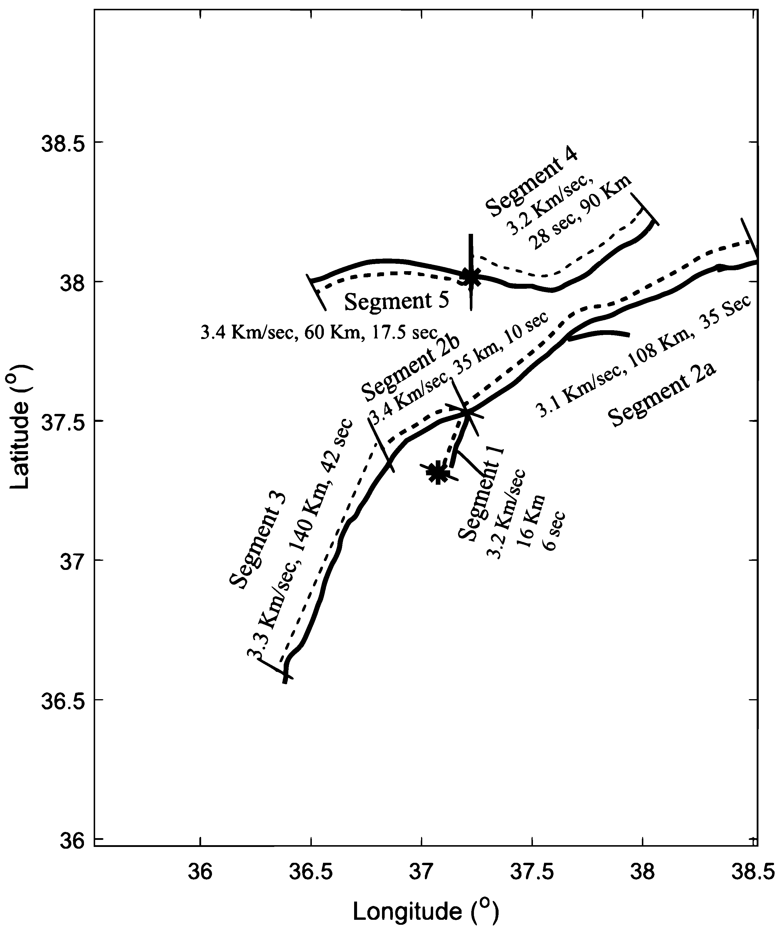
= 7.8 Kahramanmaras Earthquake    
SegmentDistance (km)Time (s)Velocity (km/s)Direction
116.06.03.2North
2 a10835.03.1North-East
2 b35.010.53.4South-West
314042.03.3South-West
M w = 7.5 Elbistan earthquake    
490.028.03.2North-East
560.017.53.4South-West
Disclaimer/Publisher’s Note: The statements, opinions and data contained in all publications are solely those of the individual author(s) and contributor(s) and not of MDPI and/or the editor(s). MDPI and/or the editor(s) disclaim responsibility for any injury to people or property resulting from any ideas, methods, instructions or products referred to in the content.

