Screening Urban Soil Contamination in Rome: Insights from XRF and Multivariate Analysis

Abstract

This study investigates spatial distribution and chemical elemental composition screening in soils in Rome (Italy) using X-ray fluorescence analysis. Fifty-nine soil samples were collected from various locations within the urban areas of the Rome municipality and were analyzed for 19 elements. Multivariate statistical techniques, including nonlinear mapping, principal component analysis, and hierarchical cluster analysis, were employed to identify clusters of similar soil samples and their spatial distribution and to try to obtain environmental quality information. The soil sample clusters result from natural geological processes and anthropogenic activities on soil contamination patterns. Spatial clustering using the k-means algorithm further identified six distinct clusters, each with specific geographical distributions and elemental characteristics. Hence, the findings underscore the importance of targeted soil assessments to ensure the sustainable use of land resources in urban areas.

1. Introduction

Soil contamination in Rome (Italy) presents a multifaceted challenge influenced by various anthropogenic activities and natural processes. Urban expansion, industrial emissions, vehicular traffic, and historical land use practices contribute to accumulating pollutants, heavy metals, hydrocarbons, and other toxicants. One significant aspect of contamination in Rome is the distribution of specific pollutants across different regions. For instance, Beryllium originates from volcanic activity in northern Latium, illustrating the contribution of geology to soil pollution [1]. Furthermore, elevated platinum levels in urban soils since 2001 highlight the impact of urbanization and the necessity for continuous monitoring to track contamination levels and spatial distribution trends [2].

Urban expansion exacerbates soil contamination in Rome, particularly in peri-urban areas—regions on the outskirts of urban centers that exhibit a mix of urban and rural land uses—where high population density leads to soil degradation and increased sensitivity to desertification [3,4]. A study on Rome’s urban expansion from 1949 to 2018 revealed a significant annual increase in urban areas, predominantly affecting high-quality soils, leading to environmental degradation [5].

Heavy metal contamination, notably of Pb, Cu, Ni, and Zn, is closely linked to vehicular traffic and urbanization in Rome, posing health risks, especially in urban parks and gardens near high-traffic roads [6]. Studies reveal that elevated levels of heavy metals and pollutants in urban soils, particularly near industrial sites and high-traffic areas, are complex and vary across different soil properties, emphasizing the need for comprehensive monitoring and remediation efforts [7]. Pollutants from industrial emissions and vehicular traffic persist in soil, posing long-term risks to human health and ecosystems. Understanding their speciation and behavior is crucial for devising effective remediation strategies and sustainable land use practices in urban areas [8].

This paper focuses on soil contamination in Rome (Italy) using XRF (X-ray fluorescence) analysis to gain insights into the distribution and characteristics of heavy metal pollutants. XRF is a widely used technique in soil contamination studies that accurately quantifies the concentration of various elements, including heavy metals, by measuring the energy and intensity of fluorescent X-rays emitted from irradiated soil samples. Studies have demonstrated strong correlations between portable XRF (pXRF) and conventional laboratory-based techniques, confirming the reliability of pXRF for soil elemental analysis in diverse environments [9]. This method is precious due to its rapid, non-destructive nature, allowing for the efficient assessment of numerous soil samples with high sensitivity and precision, even detecting trace levels of contaminants that pose environmental or human health risks. Despite some overestimations in certain elements, a study assessed the efficacy of three different pXRF scanners and found that all produced acceptable results when compared with conventional analyses across various samples, indicating the potential of XRF for reliable soil elemental analysis [10]. Also, pXRF estimates the concentration of many elements, and, when many samples are analyzed, the amount of information generated requires multivariate data science techniques.

Multidimensional scaling (MDS) visualizes similarities in datasets by projecting high-dimensional data onto lower-dimensional spaces, usually visualized by a nonlinear map (NLM) [11]. In soil analysis, this multivariate data analysis effectively represents similarities and differences in heavy metal concentrations across sampling points, aiding in understanding contamination patterns and spatial distributions. This method provides valuable insights into the factors contributing to soil contamination, significantly enhancing the region’s environmental monitoring and remediation efforts [12]. Particularly valuable in soil heavy metal contamination studies, NLM helps reveal intricate patterns and relationships between environmental factors and contamination levels, aiding in identifying hotspots and underlying processes. In China, NLM combined with neural network models have accurately predicted soil heavy metal content, while in Austria, NLM, along with fuzzy c-means cluster analysis, has effectively identified polluted areas and distinguished pollution types [13,14,15].

Principal component analysis (PCA) is commonly used to reduce the dimensionality of multivariate data, identifying significant patterns and relationships among heavy metal variables [16,17,18,19,20]. However, conventional PCA may overlook spatial heterogeneity, limiting its effectiveness. To address this, geographically weighted principal component analysis (GWPCA) was demonstrated in a study in Kumasi, Ghana, which revealed significant spatial variations not captured by conventional PCA, offering valuable insights for remediation efforts [18]. A study combining PCA, cluster analysis, and GIS in arid zones highlighted the influence of human activities on heavy metal contamination, revealing widespread pollution and informing remediation strategies [19]. A regional-scale soil contamination survey conducted in Piemonte, Italy, utilizing PCA and cluster analysis, identified heavy metal sources and assessed their natural or artificial origin. The study found that parent rocks influenced Cr, Co, and Ni, while Cu, Zn, and Pb were primarily linked to human activities [20].

Spatial clustering groups regions with similar attributes into clusters, but handling outliers (units) differing significantly from their surroundings can be challenging. A novel method, tested in Beijing, uses a sliding window to identify and decide whether to integrate or preserve outliers based on attribute variability. This approach effectively creates contiguous clusters while maintaining outliers, offering a more interpretable alternative to traditional methods [21]. The proposed method, however, effectively identifies and preserves spatial outliers, ensuring accurate identification of highly contaminated areas, which is crucial for precise mapping and practical remediation efforts.

This research mainly aimed to use portable X-ray fluorescence (XRF) instruments to evaluate the distribution of heavy metals in 59 soil samples collected from urban agricultural soils in Rome (Italy), particularly in the area outside the “Grande Raccordo Anulare” (GRA) (“Great Ring Junction”) where there is more significant potential for using urban soils for agricultural purposes [22]. Elements such as K, Ca, Ti, V, Cr, Mn, Fe, Ni, Cu, Zn, As, Rb, Sr, Zr, Mo, Sn, Ba, Ta, and Pb were analyzed. Additionally, multivariate statistical techniques, such as PCA, cluster analysis, and nonlinear mapping (NLM) were employed to classify different areas according to the concentration of chemical elements and understanding of contamination dynamics. A spatial clustering method for vector data was also introduced to handle outliers effectively. Understanding the spatial distribution of contaminants and their origins is crucial for effective remediation and sustainable land management in urban areas.

2. Materials and Methods

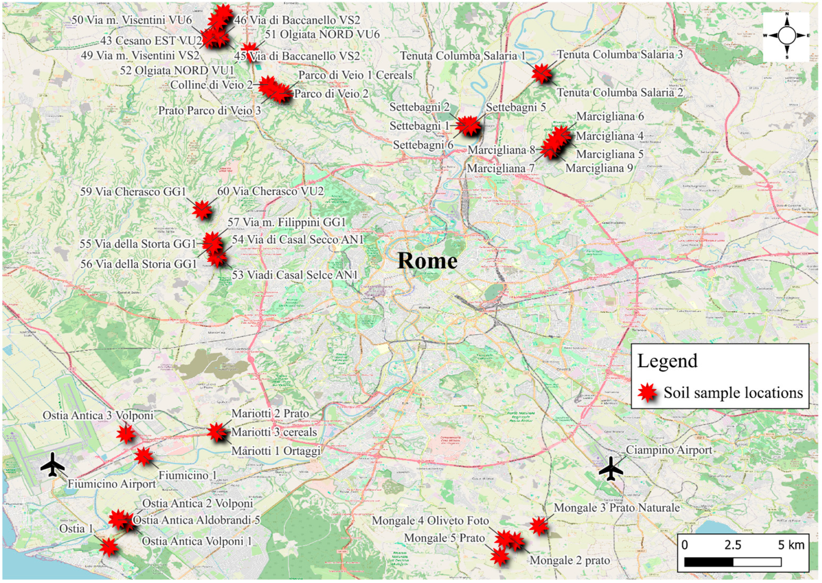
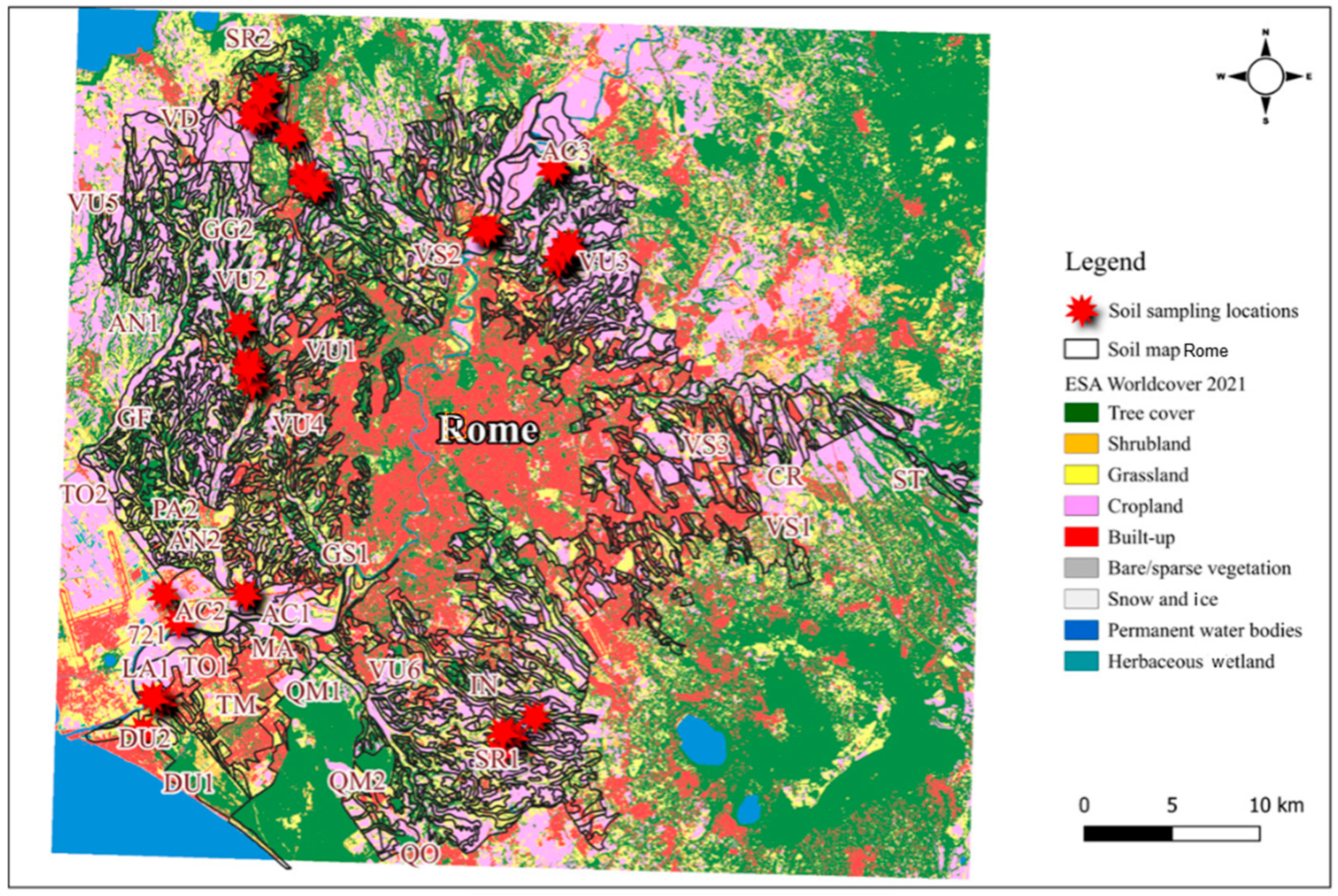
2.1. Study Area, Soil Sampling, and Sample Preparation

Figure 1 illustrates the location of the sampling points in the urban areas of Rome, Italy. Rome, one of the largest metropolitan regions in the northern Mediterranean basin, covers an area of 5365.77 km² with a population density of 788 inhabitants per km² [23]. As the third-largest metropolitan city in Italy, the Metropolitan City of Rome Capital spans nearly one third of the Lazio region, incorporating 121 municipalities. This study primarily focuses on the Rome municipality, which encompasses 150,061.3 hectares (1 hectare = 0.01 km²), particularly the 49,263.97 hectares (0.4926 km²) of arable land (QGIS 3.34) [24]. In 2023, Rome experienced typical Mediterranean climate patterns, with temperatures ranging from lows below 4.4 °C in January and December to near 32.2 °C in July and August. Rainfall was distributed throughout the year, with significant precipitation events in the winter and spring, reduced in summer, and increased again in autumn, including moderate to heavy rain and occasional thunderstorms. Wind speeds varied, with the highest gusts reaching approximately 13.4 to 17.9 m/s in early 2023, and wind directions fluctuated seasonally. Humidity levels were comfortable in cooler months and muggy in summer, peaking in July and August. Atmospheric pressure ranged from 98.0 to 103.4 kPa, being highest in January and December. These comprehensive climatic data are crucial for understanding the environmental factors influencing soil properties and heavy metal behavior in Rome [25].

In the present study, the 59 study locations for soil sampling in Italy included Ostia Antica 2 Volponi AC2 (OA2V.AC2), Mariotti 3 Cereals AC2 (M3C.AC2), Mongale 1 Cereals VS3 (M1C.VS3), Mongale 2 Prato VS3 (M2P.VS3), Ostia Antica Volponi 1 AC2 (OAV1.AC2), Colline di Veio 2 SR1 (CdV2.SR1), Fiumicino 1 (F1), Mongale 5 Prato VS3 (M5P.VS3), Mariotti 1 Ortaggi AC2 (M1O.AC2), Mongale 3 Prato Naturale IN (M3PN.IN), Ostia Antica 4 AC2 (OA4.AC2), Ostia 1 DU1 (O1.DU1), Colline di Veio 1 SR1(CdV1.SR1), Parco di Veio 1 Cereals VU4 (PdV1C.VU4), Mongale 4 Oliveto Foto SR1 (M4OF.SR1), Ostia Antica 3 Volponi (OA3V), Ostia Antica Aldobrandi 5 AC2 (OAA5.AC2), Colline di Veio 3 Soil Sottile SR1 (CdV3SS.SR1), Prato Parco di Veio 3 VU4 (PPdV3.VU4), Parco di Veio 2 VU4 (PdV2.VU4), Mariotti 2 Prato AC2 (M2P.AC2), Marcigliana 5 VU3 (M5.VU3), Tenuta Columba Salaria 2 AC3 (TCS2.AC3), Settebagni 4 AC2 (S4.AC2), Tenuta Columba Salaria 1 AC3 (TCS1.AC3), Marcigliana 8 AN2 (M8.AN2), Marcigliana 3 VU3 (M3.VU3), Settebagni 6 AC1 (S6.AC1), Marcigliana 6 VU3 (M6.VU3), Marcigliana 7 AN2 (M7.AN2), Marcigliana 9 AN2 (M9.AN2), Marcigliana 1 VU3 (M1.VU3), Marcigliana 2 VU3 (M2.VU3), Marcigliana 4 VU3 (M4.VU3), Settebagni 2 AC1 (S2.AC1), Settebagni 1 AC1 (S1.AC1), Settebagni 5 AC2 (S5.AC2), Settebagni 3 AC2 (S3.AC2), Tenuta Columba Salaria 3 AC3 (TCS3.AC3), 60 Via Cherasco VU2 (60VC.VU2), 49 Via m. Visentini VS2 (49VmV.VS2), 41 Cesano EST VU2 (41CE.VU2), 46 Via di Baccanello VS2 (46VdB.VS2), 58 Via m. Filippini GG1 (58VmF.GG1), 55 Via della Storta GG1 (55VdS.GG1), 42 Cesano EST VU2 (42CE.VU2), 54 Via di Casal Secco AN1 (54VdCS.AN1), 59 Via Cherasco GG1 (59VC.GG1), 52 Olgiata NORD VU1 (52ON.VU1), 53 Viadi Casal Selce AN1 (53VCS.AN1), 44 Cesano EST VU2 (44CE.VU2), 57 Via m. Filippini GG1 (57VmF.GG1), 47 Via di Baccanello VS2 (47VdB.VS2), 48 Via di Baccanello VS2 (48VdB.VS2), 45 Via di Baccanello VS2 (45VdB.VS2), 50 Via m. Visentini VU6 (50VmV.VU6), 51 Olgiata NORD VU6 (51ON.VU6), 43 Cesano EST VU2 (43CE.VU2), and 56 Via della Storia GG1 (56VdS.GG1). The characteristics of the 59 sampling locations are described in Table S1.

In 2023, a total of 59 agricultural soil samples were collected from the upper 30 cm surface layer using a drill in three separate batches (April, May, and July) from Rome, Italy, encompassing various land uses, such as tree cover, shrubland, grassland, cropland, and built-up areas. Figure 1 illustrates the study area for these soils. A composite sample (1 kg of soil) was taken at each site, comprising 15–20 subsamples. These samples were placed in airtight polyethylene bags, labeled with coordinates, location names, and cultivation types, and transported to the laboratory for analysis [22]. Primary geographic data were obtained from Google Earth and QGIS 3.34 [24]. The first and second batch soils were dried at room temperature for 1–2 weeks, while the third batch soils were dried in a hot air oven at 60 °C for two days. After drying, all soils were passed through a 2 mm stainless steel sieve to remove debris and stone fragments. The weights of the fine earth and stone fragments were measured and recorded. The fine earth was then split into two halves and stored in Ziploc bags, with one half designated for immediate laboratory experiments and the other for future use.

The study area encompasses the territory within the municipality of Rome, Italy. The Urban Atlas of Rome is a vector file representing land use, including agricultural areas, within the metropolitan area of Rome. Agricultural land is classified under class 2 with a minimum mapping unit of 1 hectare, and the target class is 21,000 arable land (annual crops) [22,26]. To reconstruct the CTR mosaic (Carta Tecnica Regionale or Regional Technical Map), all the raster CTR files covering Rome’s municipality area were downloaded (shown in the background of the soil map). These data were sourced from the Lazio Pedological Map and the Index of Cartografia CTR_10K_TIF ROMA LIMITI [26,27]. The soil map was then georeferenced using EPSG 3004, and the digitization process was completed using free QGIS software 3.34 by digitizing the mapped polygons (Figure 2). Various soil types in this region were summarized based on information from the “Carta dei Suoli del Comune di Roma in scala 1:50.000-I SUOLI DI ROMA Due passi sulle terre della città” (soil map of the municipality of Rome) [22,28]. Selected sites within the Rome municipality, featuring diverse soil types and land uses, were identified using Google Earth and Google Maps. A comprehensive list of urban farm locations was compiled, including addresses, email contacts, and phone numbers. Contact was established with these farms to seek cooperation for soil surveying, and permission from landowners was obtained for sample collection.

2.2. XRF Analysis

For the XRF analysis, the soil samples were air-dried, oven-dried, and sieved through a 2 mm mesh to minimize the effects of moisture, heterogeneity, and particle size on the analysis [29,30,31,32,33]. The concentrations of various elements in the 59 soil samples were quantified using the X-MET7000 handheld energy dispersive X-ray fluorescence (EDXRF) analyzer on a benchtop stand, and the software SW Version 1.1B.7580 was used (Oxford Instruments, Abingdon, Oxfordshire, UK).

Each soil sample (0.400 and 0.800 g) was placed in a sample cup, and three consecutive readings were taken, with the sample cup (plastic cylinder box with open edges sealed by a plastic tape) repositioned over the scanner’s measurement window for each reading. All these materials were provided by the manufacturer of the instrument. The readings were averaged to obtain the final elemental concentrations.

The analysis time was 60 s. The soil analysis method was used, which has a relatively large elemental detection range. The system was calibrated using a combination of fundamental parameters (FP) methods and the automatic selection of empirical calibrations (certified reference materials). The energy resolution of the system was <145 eV and the concentration of each element was automatically delivered in ppm, as well as the correspondent sample spectrum [34].

The elements analyzed included potassium (K), calcium (Ca), titanium (Ti), vanadium (V), chromium (Cr), manganese (Mn), iron (Fe), nickel (Ni), copper (Cu), Zinc (Zn), arsenic (As), rubidium (Rb), strontium (Sr), Zirconium (Zr), molybdenum (Mo), tin (Sn), barium (Ba), tantalum (Ta), and lead (Pb). This methodology ensured high precision and accuracy in the elemental quantification of the soil samples. Table S2 shows the XRF results obtained from the 59 soils in Rome, Italy.

The results of the concentrations measured by the portable XRF equipment may raise some doubts [9,10]. Besides the internal calibration procedures already described above, a comparison of the results previously obtained by ICP-MS and already published [22], with those obtained by pXRF for the same subset of eleven soils were compared for the elements V, Cr, Ni, Cu, Zn, Ba and Pb, and a linear trend between the two measurements was observed with the following correlation coefficients: 0.972, 0.924, 0.960, 0.897, 0.901, 0.977, and 0.906, respectively.

2.3. Descriptive Statistics and Multivariate Analysis

Descriptive statistics, including measures such as mean, maximum, minimum, median, Quartile 1, Quartile 3, skewness, kurtosis, the Kolmogorov–Smirnov (K–S) test, and the coefficient of variation (CV), were computed using the free software R 4.3.3 version (RStudio) [35]. The Kolmogorov–Smirnov test was used to assess the normality of the variable distributions [36], and the coefficient of variation was employed to estimate the variability in Potentially Toxic Elements (PTE) concentrations.

For the multivariate analysis of the 59 soil samples obtained via XRF analysis, a series of unsupervised multivariate techniques were employed to explore and understand the clustering and dimensionality of the data using the R 4.3.3 software (RStudio) [35]. Initially, the ALSCAL procedure for multidimensional scaling was used to generate a nonlinear map (NLM), providing an exploratory analysis of clustering patterns. Principal component analysis (PCA) was computed from the variance–covariance matrix of the original variables and was used to project the data onto the space defined by the first three significant eigenvectors [18,37,38,39,40,41,42,43]. Hierarchical cluster analysis (HCA) was subsequently conducted to examine the characteristics of each cluster, enhancing the understanding of the data structure and identifying distinct clusters. HCA was used with the complete linkage method and the Lance–Williams dissimilarity update formula.

2.4. Spatial Clustering

Spatial clustering is essential as it considers geographic proximity, leading to more meaningful insights specific to locations. In addition to HCA, spatial clustering using the k-means algorithm was performed in Python 3.10 [44].

For the spatial clustering analysis of soil heavy metals, the study area encompassed Rome’s urban and peri-urban regions. Soil samples from 59 locations across Rome were collected and analyzed using k-means clustering with six clusters. This number of six clusters resulted from the previous PCA and HCA analysis of the full data set and from a final optimization resulting from a trial and error approach until coherent spatial results were obtained. This method accounted for the exact geographic coordinates of each sample collection point, providing a comprehensive analysis of the spatial distribution of the soil samples. The clustering results were then analyzed to assess the spatial distribution patterns of soil heavy metals across Rome, offering valuable insights into potential sources and spatial variability.

Spatial clustering was performed directly on the vector data (59 samples) using k-means clustering with six clusters. k-means clustering was applied to group geographical locations in Rome, Italy, based on standardized features. The dataset was prepared by removing irrelevant columns, such as serial numbers and soil names, focusing solely on quantitative attributes that influence location characteristics. The data were standardized using Standard Scaler from the “scikit-learn” library to ensure each feature contributed equally to the model. We then used the k-means algorithm, specifying six clusters to identify inherent groupings in the data. A random seed was set to ensure the reproducibility of results.

Following the clustering, we visualized the geographical distribution of the clusters by plotting each location on top of OpenStreetMap using QGIS, differentiated by cluster identities using a distinct color palette. This visualization facilitated the interpretation of spatial patterns and the distribution of clusters across geographical areas, demonstrating the utility of machine learning techniques in uncovering meaningful patterns from complex, multidimensional datasets.

3. Results and Discussion

3.1. Descriptive Statistics for XRF Contents in Soil Samples

The descriptive statistics for the XRF contents in the 59 soil samples reveal significant variability in the concentrations of various elements.

Table 1. Summary of descriptive statistics for XRF contents (mg/kg) in soil samples of the present study.

	K	Ca	Ti	V	Cr	Mn	Fe	Ni	Cu	Zn	As	Rb	Sr	Zr	Mo	Sn	Ba	Ta	Pb
Mean	15,938	39,995	5143	274	997	1175	42,435	229	43	71	8	275	640	282	7	3	200	15	89
Minimum	3191	6058	2352	<LD	<LD	441	17,612	<LD	<LD	23	<LD	50	221	65	<LD	<LD	<LD	<LD	<LD
Q1	14,224	15,188	3804	110	<LD	914	36,205	21	20	62	<LD	158	336	176	<LD	<LD	166	<LD	44
Median	16,417	25,285	4327	172	68	1120	40,881	28	30	69	<LD	247	510	325	<LD	<LD	224	19	71
Q3	18,056	71,126	5114	214	102	1376	50,018	43	46	80	20	372	799	366	<LD	<LD	266	25	83
Maximum	31,316	123,059	17,816	1957	15,122	2163	62,414	3512	304	118	35	781	1829	437	110	47	415	75	933
Skewness	0.01	0.72	3.13	3.34	3.50	0.68	0.23	3.58	3.33	0.32	1.09	0.97	1.29	−0.36	3.45	3.48	−0.75	1.06	5.64
Kurtosis	4	2	12	13	13	3	3	14	16	4	2	4	4	2	13	13	3	4	38
K-Sp	0.17	0.01	<0.01	<0.01	<0.01	0.70	0.37	<0.01	<0.01	0.36	<0.01	0.51	0.07	0.08	<0.01	<0.01	0.14	<0.01	<0.01
CV [%]	35	79	61	154	354	32	24	329	111	25	165	53	63	38	374	375	53	115	140

Q1—lower quartile; Q3—upper quartile; K-Sp—Kolmogorov–Smirnov; CV—coefficient of variation; LD—limit of detection.

summarizes the descriptive statistics for all the elements studied in Rome as per the combined results of all 59 study locations. Calcium (Ca) and iron (Fe) are the most abundant elements, with mean concentrations of 39,995 mg/kg and 42,435 mg/kg, respectively. These elements show moderate variability, as indicated by their coefficients of variation (CV) of 79% for Ca and 24% for Fe. In contrast, several elements demonstrate extreme variability. Molybdenum (Mo) and Tin (Sn) have the highest CVs at 374% and 375%, respectively, indicating that their concentrations are highly inconsistent across the soil samples. This suggests significant heterogeneity, possibly due to localized contamination or varying geochemical conditions.

Vanadium (V) and lead (Pb) also exhibit notable variability, with CVs of 154% and 140%, respectively, suggesting heterogeneous distribution across the samples, pointing to natural and anthropogenic influences. Similar findings were obtained by Unsal et al. [40] and Chandramohan et al. [22], where elements like Zn and Pb showed high variability due to localized contamination.

Lead (Pb) shows the highest skewness and kurtosis among all the elements, indicating a highly asymmetrical, peaked distribution with extreme outliers, suggesting significant variability in Pb concentrations. The high kurtosis and skewness values for elements like nickel (Ni), titanium (Ti), and chromium (Cr) indicate the presence of outliers and non-normal distribution, suggesting specific geological formations or contamination hotspots, aligning with observations of skewed metal distributions in other regions [16,45]. Zinc (Zn) and manganese (Mn) show lower variability, with 25% and 32% CVs, respectively.

The data indicate that the soil samples are characterized by a wide range of elemental concentrations, with some elements like Mo and Sn displaying exceptionally high variability. These findings suggest diverse and variable elemental presence in the soil, which could be attributed to natural and anthropogenic factors. This study’s portable X-ray fluorescence (pXRF) application is consistent with earlier findings that underscore its effectiveness and limitations. Shand and Wendler [46] reported that pXRF provided reliable results for elements like Cu and Pb but tended to overestimate the concentrations of others, such as Ca, Ti, and Fe, highlighting the importance of meticulous calibration. Similarly, Caporale et al. [14] found strong correlations between pXRF and traditional aqua regia extraction for several metals. However, pXRF often recorded higher concentrations, likely due to the incomplete dissolution of metal-bearing silicates during the aqua regia extraction process.

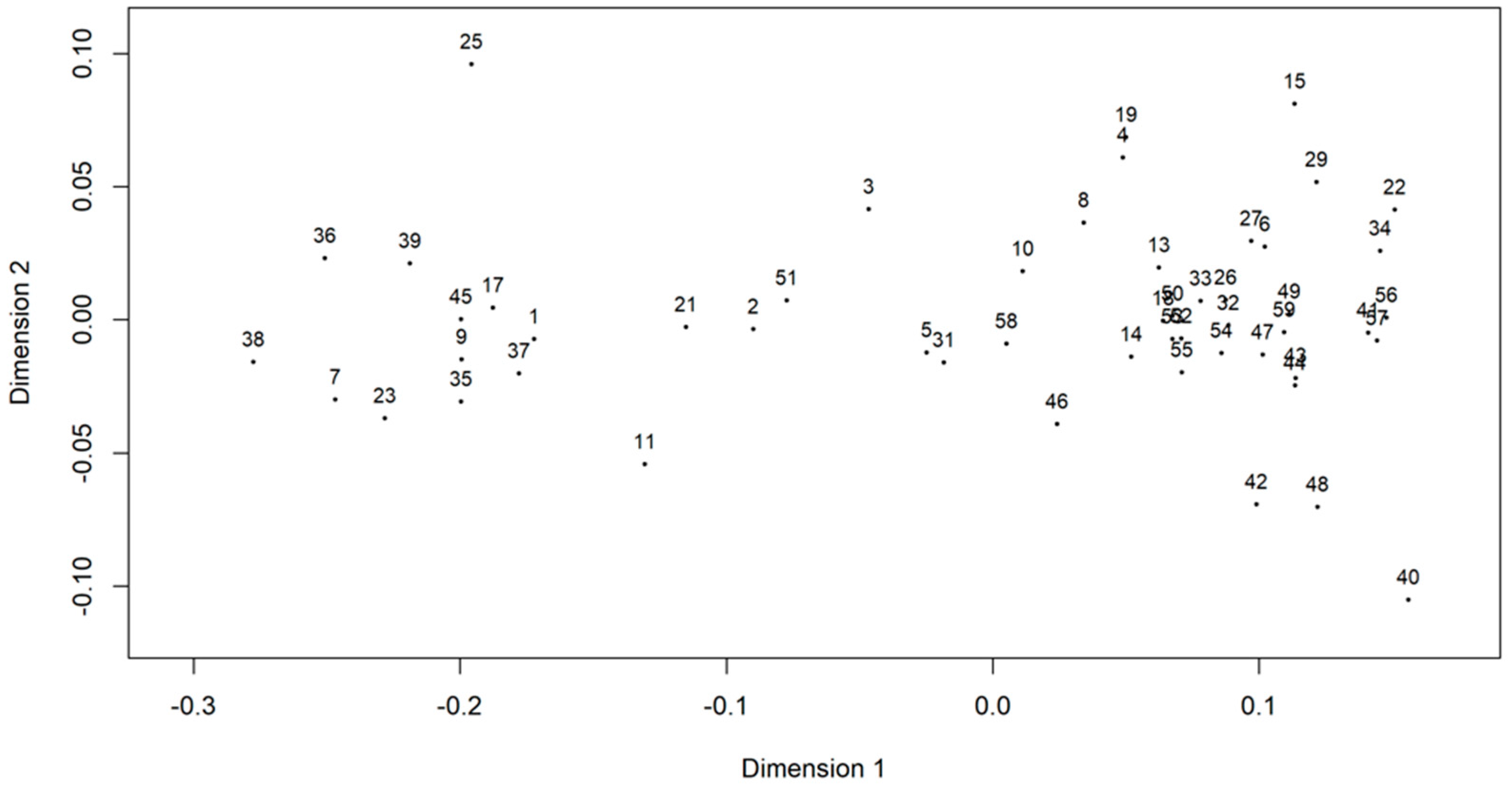
3.2. Nonlinear Multidimensional Scaling (NLM)

The NLM analysis using the ALSCAL algorithm adds another dimension to understanding the similarities and dissimilarities among the soil samples. The configuration plot reveals distinct clusters consistent with PCA and hierarchical clustering findings. Closely grouped samples indicate high similarity in their elemental compositions, while outliers, such as sample 40, suggest unique profiles. The ALSCAL algorithm’s capability to handle various types of data and its flexibility in applying different models, as described by Young et al. [10], reinforces the identification of these distinct groups and unique samples within the dataset, thus supporting the robustness of our findings.

The ALSCAL algorithm, by creating geometric representations of the data, allows for a nuanced understanding of how soil samples relate to each other based on their elemental compositions. The primary strength of MDS (multidimensional scaling), as performed by ALSCAL, lies in its ability to reduce the complexity of the dataset and present the data in a visually interpretable form [9], highlighting distinct clusters of similar items (in this case, soil samples) and outliers, providing clear evidence of differences in soil composition that other statistical techniques might miss. A study by Carlotto [11] reported that the ALSCAL algorithm is particularly effective for visualizing complex, high-dimensional data by reducing it to a lower-dimensional space while preserving crucial relationships between data points. This capability is vital for identifying patterns, such as clustering and outliers; other analytical methods may overlook this. Further, a study by Hanesch et al. [13] demonstrated that NLM is particularly effective in distinguishing between polluted and unpolluted soil samples by revealing complex relationships between variables, such as magnetic susceptibility and heavy metal content, that may not be apparent through more straightforward statistical methods, thus aiding in environmental impact assessment. In addition, a study by Duan et al. [12] demonstrated the effectiveness of various neural network models in predicting soil heavy metal content, highlighting the significance of incorporating advanced algorithms for improved accuracy in environmental monitoring. Finally, NLM’s ability to preserve data structure during dimensionality reduction is invaluable for identifying and visualizing clusters in high-dimensional datasets [47].

The results from the NLM, as illustrated in Figure 3, provide a clear visualization of the multidimensional relationships among the 59 soil samples, reduced to a two-dimensional space. The plot reveals several distinct clusters, indicating that certain groups of soil samples share similar elemental compositions or properties. For example, samples 1, 9, 17, 35, 37, and 45 are clustered together and form a tight group in the left-central region of the plot, suggesting that they have closely related elemental profiles. In the multidimensional scaling plot, the samples labeled 38, 36, 39, 7, 23, 35, 37, 1, 17, 45, and 9 form a distinct cluster in the left-central region, indicating significant similarities.

On the right side of the multidimensional scaling plot, a subgroup of samples, including labels 13, 14, 55, 50, 52, 18, 32, 33, 26, 54, 47, 59, 49, 44, 43, 6, and 27, is tightly clustered, indicating significant similarity among these samples. This subgroup is positioned within a larger, more diffuse group composed of samples 42, 48, 57, 41, 56, 34, 22, 29, 15, 19, 4, 8, 10, 58, and 46. The presence of this subgroup within the broader cluster suggests that, while the samples share some common characteristics, the subgroup exhibits a higher degree of internal homogeneity. This pattern may reflect a hierarchical structure in the data, where the subset represents a more specific condition or feature set within the broader context of the larger group’s shared characteristics. Further analysis is needed to understand the factors driving this internal structure and the relationship between the subgroup and the larger group.

Additionally, the NLM analysis identifies outliers, such as samples 11 and 40, which are isolated from the main clusters. For instance, sample 40 is positioned far from other samples, suggesting it has a unique elemental composition compared to the rest. These outliers indicate that these samples possess unique characteristics or significantly different elemental profiles compared to the other samples. The spread along Dimension 1 in the plot suggests a gradient of a specific elemental property or a combination of properties, further differentiating the samples.

However, other samples, like 25, 42, 48, 3, and 15, exhibit distinct positions that provide insights into their elemental compositions. Sample 25, potentially located near the edge of a larger cluster, suggests it shares similarities with the central group but also possesses unique characteristics that could serve as a bridge between different soil profiles. Samples 42 and 48 form a small cluster within the broader right-side group, indicating a close relationship but with potentially unique attributes compared to the rest of the group, reflecting similar environmental conditions or geological origins. In contrast, sample 48 likely has a unique elemental profile, possibly due to specific local factors such as anthropogenic influence or distinct geological formations. Sample 3, if found near multiple clusters, suggests overlapping characteristics with different groups, indicative of a transitional profile where it shares features with soils from varying environments. Sample 15, depending on its placement, could either reinforce its association with a central cluster or highlight its distinctiveness, suggesting unique environmental or geochemical influences. These interpretations underscore the complexity and variability in the soil samples, driven by both natural and anthropogenic factors.

These distinct clusters and outliers indicate variability in the soil’s elemental composition, which could be attributed to different geological origins, varying levels of contamination, or other environmental factors influencing the soil composition. The NLM plot thus effectively highlights the complexity of the soil samples’ relationships and provides insights into potential factors contributing to the observed variability in their elemental compositions.

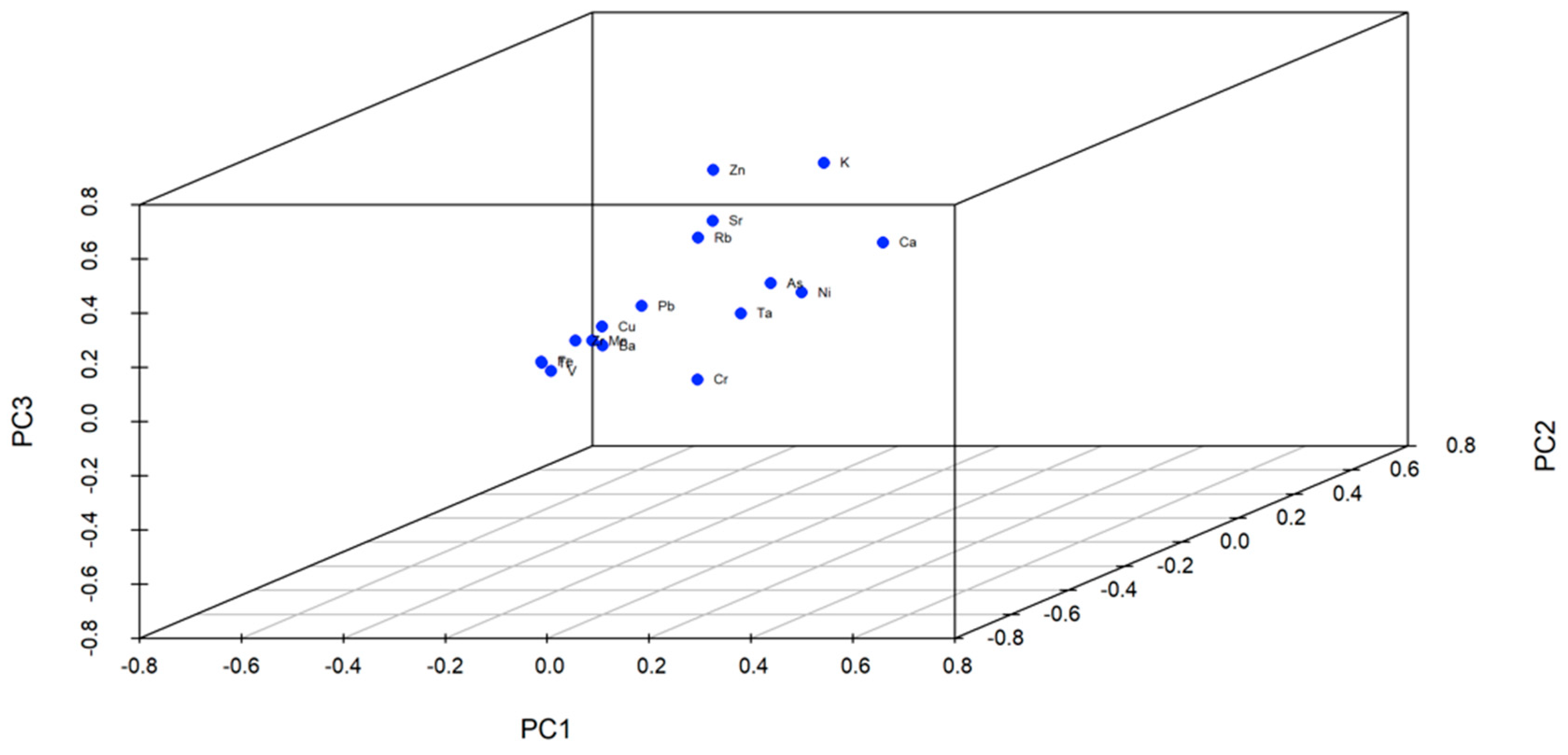
3.3. Principal Component Analysis (PCA)

PCA was conducted to reduce the dimensionality of the data and identify the key components that explain the most variance within the soil sample dataset. For example, PCA has been applied to assess metal distribution in agricultural soils and vegetables, as seen in Balabanova et al. [48], and to identify key contamination sources in urban soils, as demonstrated by Wieczorek et al. [45] in Poland. Finally, Han and Li [49] used PCA to differentiate industrial from natural sources of contamination in Xining, China, and Ahmed et al. [50] highlighted the impact of industrial activities and vehicular emissions on metal concentrations in soils along the Dhaka Aricha Highway in Bangladesh.

The first three principal components (PCA 1, PCA 2, and PCA 3) account for variances of 0.3837, 0.2308, and 0.1096, respectively. The first two components explain 61% of the total variance, while the first three increase this cumulative variance explanation to 72%.

The 3-dimensional loadings plot (Figure 4) reveals the distribution of the soil samples across the first three principal components. The plot shows that the first component (PCA 1) captures the most significant variation in the data, followed by PCA 2 and PCA 3. For example, the 3D loadings plot of the first three principal components (PC1, PC2, and PC3) reveals that elements like Ca, As, Ni, Cr, and Ta significantly contribute to PC1. At the same time, K, Zn, Rb, and Sr are more influential on PC2, and Zn, Fe, V, and Ti contribute notably to PC3.

These contributions indicate the roles these elements play in explaining the variance within the dataset across the different dimensions represented by the principal components. Further, the score plots in the S.I. (PC1 vs. PC2, PC1 vs. PC3, and PC2 vs. PC3) demonstrate the distribution of soil samples, highlighting variability and potential clustering based on their elemental compositions.

The 3D loadings plot reveals a distinct clustering of elements based on their contributions to the three principal components. Elements such as Fe, Ti, and V are tightly clustered near the origin, suggesting similar loading patterns and contributions to the variance captured by the components. In contrast, elements like K and Ca are more distantly positioned, indicating unique contributions, with K primarily associated with PC2 and PC3 and Ca with PC1. A moderate cluster involving Pb, Cu, Ba, Rb, and Sr suggests shared variance contributions among these elements, alongside PC1 and PC2. Zn and K are positioned relatively far from the central cluster, indicating they have unique loading patterns, particularly along PC3 for Zn and PC2 for K, suggesting that these elements have distinct influences on the variance along these components compared to other elements.

Calcium (Ca) and nickel (Ni) have significant loadings along PCA 1, indicating they are major drivers of the variability captured by this component. Similarly, potassium (K) and zinc (Zn) are strongly associated with PCA 2 and PCA 3, respectively. Moreover, clusters of samples in a similar PCA plot indicate groups of soil samples with similar elemental compositions, which implies that these samples originate from similar geological environments or are influenced by comparable contamination sources.

The loadings plot for PC1 vs. PC2 in Figure S1 from S.I. provides a detailed visualization of how different elements contribute to the variance captured by the first two principal components, which together account for 61% of the total variance (38% by PC1 and 23% by PC2). This plot helps visualize the separation of samples based on their elemental profiles, with distinct clusters likely representing different soil types or contamination levels. The loadings plot illustrates the contributions of various elements to the first two principal components (PC1 and PC2). Elements like calcium (Ca) and nickel (Ni) are positioned far along the positive axis of PC1, indicating that they contribute significantly to the variance captured by this component and may be critical drivers differentiating the soil samples based on their concentrations. Conversely, elements such as titanium (Ti), iron (Fe), and vanadium (V) are found along the negative axis of PC1, suggesting they contribute differently to the variance compared to elements on the positive axis, potentially reflecting distinct geochemical or environmental influences. The proximity of elements in the plot also indicates their correlations. For instance, elements like strontium (Sr) and rubidium (Rb) are closely grouped near the positive end of PC2, implying a positive correlation between these elements in the soil samples.

Similarly, zinc (Zn) and tantalum (Ta), positioned close together, suggest that these elements tend to vary together across the samples. The distinct positioning of chromium (Cr) along the positive PC1 axis, separate from other elements, suggests that Cr has a unique contribution to the variance captured by this component, possibly indicating a specific source or environmental process influencing its distribution in the soils. Meanwhile, elements like lead (Pb) and manganese (Mn), situated along the negative PC2 axis, may indicate their role in a separate variation pattern captured by this component, potentially reflecting contamination or specific geochemical processes.

The loadings plot for PC1 vs. PC3 in Figure S2 illustrates how the elements contribute to the variance captured by the first and third principal components, which explains 49% of the total variance (38% by PC1 and 11% by PC3). This plot provides additional insights into the differentiation of soil samples that still need to be captured by two principal components that may not be fully captured. Calcium (Ca) and nickel (Ni) are distinctly positioned along the positive axes of PC1 and PC3, indicating their significant contributions to the variability in the dataset. Their positioning suggests they play a crucial role in differentiating certain soil samples, potentially due to specific geological or environmental processes. Additionally, zinc (Zn) and potassium (K) are notably positioned along the positive PC3 axis, with zinc having a powerful influence, suggesting it significantly contributes to the variance captured by PC3 and may reflect unique soil characteristics or localized contamination not as powerfully captured by the first two components. Strontium (Sr) and rubidium (Rb), grouped along the positive PC3 axis, continue to show a positive correlation in this component, similar to the PC1 vs. PC2 plot. Conversely, titanium (Ti), iron (Fe), and vanadium (V) are clustered along the negative axes, indicating an inverse relationship with elements on the positive axes, particularly in their contribution to the third component’s variance. This plot reveals essential differences in elemental donations that may need to be apparent in the PC1 vs. PC2 plot. For instance, the distinct separation of chromium (Cr) along the positive PC1 axis, with a moderate contribution to PC3, indicates a unique role in soil composition, partially captured by the third component.

The loadings plot for PC2 vs. PC3 in Figure S3 highlights how the elements contribute to the variance captured by the second and third principal components, which account for 34% of the total variance (23% by PC2 and 11% by PC3). This plot provides additional insights into the variability within the soil samples that the first principal component may not fully capture. Zinc (Zn) and calcium (Ca) are positioned prominently along the positive PC3 axis, with zinc strongly influencing the third component. This suggests that these elements contribute significantly to the variance captured by PC3, highlighting their importance in differentiating certain soil samples, possibly due to specific environmental or contamination factors. Elements such as strontium (Sr) and rubidium (Rb) are closely grouped along the positive PC2 axis, similar to their positioning in previous plots, reinforcing their strong positive correlation in the dataset. Potassium (K) is also aligned along the positive PC2 axis but at a different position, indicating that while it is positively correlated with Sr and Rb, it contributes uniquely to the variance captured by PC2. On the opposite end, elements like chromium (Cr), iron (Fe), and titanium (Ti) are clustered together along the negative axes of PC2 and PC3. This positioning suggests that these elements contribute differently to the variance, reflecting different sources or environmental processes influencing their distribution in the soil samples. Arsenic (As) is distinctively positioned along the positive PC2 axis, suggesting it plays a unique role in the variance, possibly due to localized contamination or specific geochemical processes.

Similar studies have successfully used PCA to differentiate between natural and anthropogenic sources of soil contaminants. For example, Borůvka et al. [16] identified Co, Cr, Cu, Ni, and Zn as geogenic, while Pb, Cd, and Hg were mainly anthropogenic in the Czech Republic. Similarly, Bretzel and Calderisi [38] found significant metal contamination in urban soils near roads, particularly from lead and zinc, due to traffic pollution. Chang et al. [51] utilized PCA to reveal distinct patterns of heavy metal contamination in road dust and soil influenced by local industrial activities. Moreover, Lu et al. [17] demonstrated PCA’s utility in optimizing air quality monitoring networks and effectively identifying pollution behaviors and emission sources. This approach was also employed by Mali et al. [52] in the Gulf of Naples, where PCA reduced environmental data complexity and highlighted vital factors contributing to pollution in coastal areas. At the same time, Salvati [53] used PCA to explore the impact of urban expansion on soil quality in Rome, revealing a gradient from urbanized areas to agricultural lands. In the Nile Delta, El Behairy et al. [19] used PCA to differentiate between natural and anthropogenic sources of pollution, while Krami et al. [54] highlighted the effectiveness of PCA in environmental pollution studies in Iran. Similarly, using PCA, Kahangwa [55] identified natural and anthropogenic contamination sources in soils from Tanzanian gold mining areas.

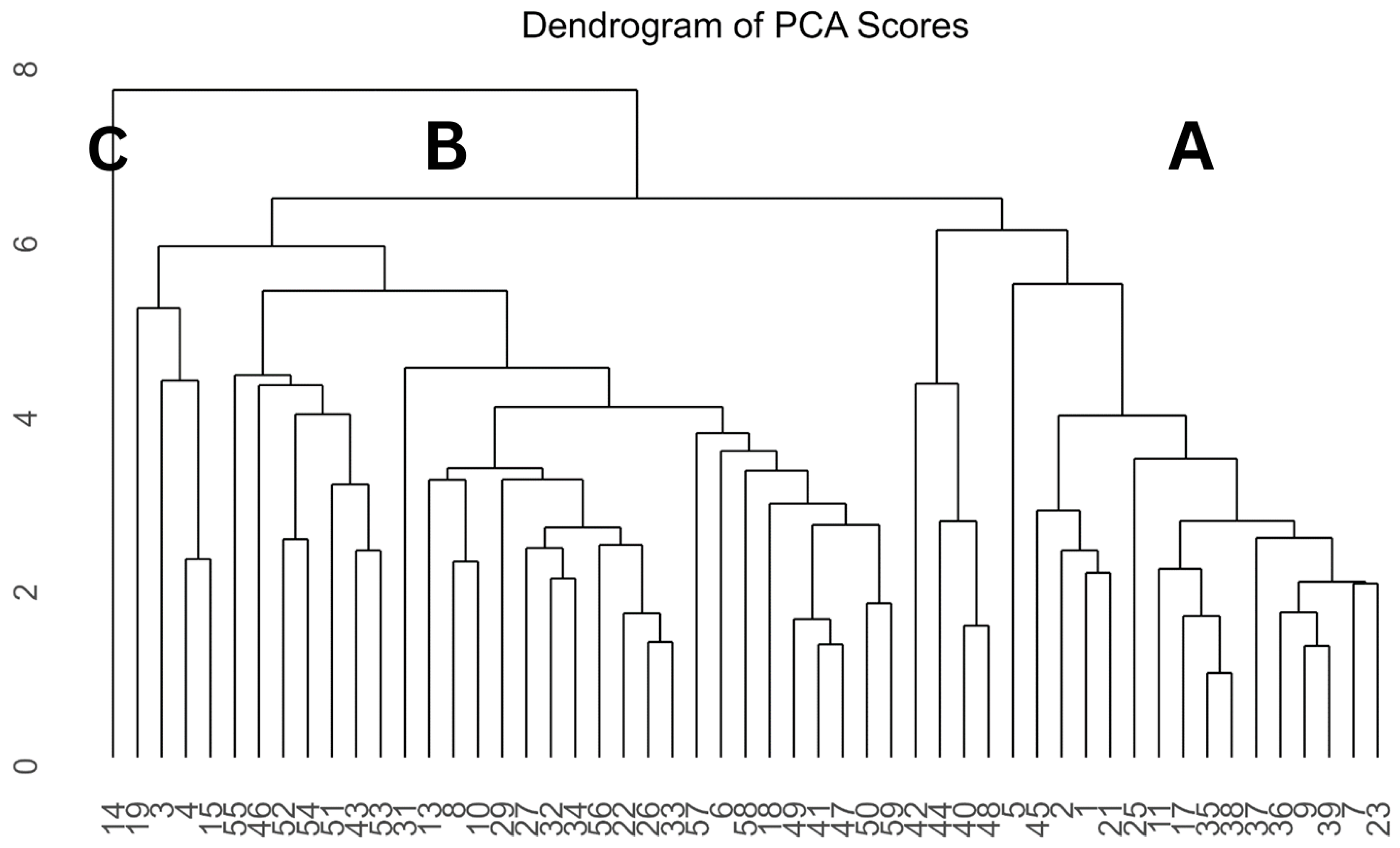
3.4. Hierarchical Cluster Analysis Based on PCA Scores

The hierarchical clustering dendrogram provides a clear hierarchical structure of the soil samples, reflecting their elemental similarities. The significant clusters identified similar samples, while the further subdivisions revealed more detailed clusters. The hierarchical approach complements the PCA results, confirming the distinct groups and highlighting the relationships among the soil samples. The PCA and HCA provided valuable insights into the underlying structure of the soil dataset. The distinct clusters identified in both analyses correspond to geographical locations, suggesting that different areas within the Roman territories had unique geochemical signatures. This spatial differentiation can be attributed to varying soil formation processes, historical land use patterns, and potential localized contamination sources. These results align with earlier research where HCA has effectively categorized environmental samples based on contamination profiles.

For instance, Mali et al. [52] used HCA to categorize sediment samples from the Gulf of Naples, revealing the spatial distribution of pollutants and the influence of natural and anthropogenic factors. Similarly, Lu et al. [17] optimized the air quality monitoring network in Hong Kong by using HCA to group stations based on pollution behaviors, highlighting geographical factors influencing pollution patterns. El Behairy et al. [19] applied HCA to soil samples from the Nile Delta, distinguishing between areas impacted by industrial and agricultural activities and highlighting the significant anthropogenic influence on soil quality. In Iran, Krami et al. [54] used HCA to reveal the spatial variability of contamination sources in Hamedan County, linking distinct metal groups to natural or anthropogenic origins. Kahangwa [55] employed HCA in Tanzania to identify different clusters of soil samples from gold mining areas, effectively distinguishing between anthropogenic and natural contamination sources. Han and Li [49] also used HCA in Xining, China to differentiate between areas impacted by industrial activities and natural sources, revealing distinct clusters based on heavy metal concentrations. Finally, Ahmed et al. [50] applied HCA along the Dhaka Aricha Highway in Bangladesh, revealing clusters that provided insights into the spatial distribution of contamination, particularly highlighting the influence of vehicular emissions and industrial activities on soil quality. These studies collectively underscore the robustness of HCA in environmental monitoring and its ability to reveal spatial contamination patterns, supporting our research findings.

Figure 5, the hierarchical dendrogram of the Roman samples, provides a detailed visualization of the relationships and similarities among the 59 soil samples based on their PCA scores. The complete linkage method was used for clustering, which maximizes the distance between the most dissimilar members of each cluster. This method was used because it originates balanced dendrograms, i.e., the clusters are easily observed and classified. The hierarchical clustering dendrogram based on PCA scores illustrates the relationships among the soil samples, grouping them into clusters and subclusters based on their similarity in elemental composition. The vertical axis represents the dissimilarity between clusters, with higher values indicating more significant dissimilarity. The dendrogram reveals several distinct main clusters, indicating groups of soil samples that share similar elemental profiles. The larger clusters suggest that these samples are more closely related to each other regarding their overall elemental composition.

The HCA dendrogram shows two major clusters, with further subdivisions indicating more specific groupings. Cluster A, for example, includes samples like 42, 5, 25, 37, 7, and 23, which share similar PCA scores and elemental compositions, while Cluster B consists of samples such as 19, 55, 31, 57, up to 59, forming another distinct group. Within each central cluster, the dendrogram further divides the samples into subclusters. These subclusters represent finer distinctions within the main groups, suggesting that while the samples in each central cluster are similar, there are still differences in their specific elemental compositions. For example, within Cluster A, samples 42, 44, 40, and 48 form one subcluster, and samples from 5 to 23 form another subcluster. Similarly, Cluster B has subclusters with samples like 19, 3, 4, and 15 grouped closely together, reflecting a higher similarity, while other subclusters (samples from 55 to 59) within the same central cluster represent different but related soil compositions. Cluster A and Cluster B unite and then combine with the third Cluster C with sample 14 on a larger scale.

The dendrogram shows no extreme outliers wholly isolated from the other clusters. However, samples that branch off early from the main clusters, typically at higher positions in the dendrogram, may be considered less similar to most samples in their cluster. Samples on the dendrogram’s extreme left or right ends may also exhibit distinct characteristics.

3.5. Spatial Clustering of Soil Samples

The spatial clustering results provide valuable geographical insights into the distribution of soil samples based on their elemental compositions. The clusters identified through k-means clustering highlight regions with similar soil characteristics, suggesting spatial patterns influenced by environmental, geological, or anthropogenic factors. This spatial analysis underscores the importance of considering geographical factors in understanding soil composition and distribution. This approach aligns with the findings of Wang et al. [21], who introduced a raster-based spatial clustering method, robust against spatial outliers, which effectively groups spatial units while preserving outliers, thereby ensuring accurate spatial analysis, even in the presence of extreme variations.

Moreover, spatial clustering has broad applications across different fields, as highlighted by various studies. For instance, Wang et al. [56] used spatial clustering to analyze urban signatures in precipitation extremes across Mainland China, while Yu et al. [57] applied the technique to nighttime light satellite images to delineate urban spatial clusters and assess landscape patterns. These applications demonstrate the versatility and utility of spatial clustering in environmental and urban studies, reinforcing the significance of considering geographical factors in understanding soil composition and distribution. This study applied k-means clustering to group 59 geographical locations in Rome, Italy, based on various standardized features.

The clustering analysis revealed distinct spatial patterns in the soil samples, visualized in the map with OpenStreetMap in the background (Figure 6). For data preparation, irrelevant columns, such as serial numbers and soil names, were removed from the dataset. Later, the dataset was standardized using the StandardScaler from the sci-kit-learn library, ensuring each feature had a zero mean and unit variance. For k-means clustering, the k-means algorithm was implemented with six clusters to identify inherent groupings in the data, and a random seed was set to ensure reproducibility of the results.

The map shows the geographical distribution of the clusters, with each location represented as a point. Figure 6 illustrates different clusters indicated by distinct colors, as shown in the color legend on the right of the map. As there is a bit of overlapping between a few clusters, half the clusters (Cluster 0, Cluster I, and Cluster III) are shown on the left-side map and the other half (Cluster II, Cluster IV, Cluster V) are shown on the right-side map.

Using the k-means algorithm, the spatial clustering identifies six distinct clusters, each with specific geographical distributions.

-

Cluster 0 (pink): Mostly located in the northern and southwestern parts of the study area. The close grouping of points suggests that these locations share similar soil characteristics;

-

Cluster I (light green): These are primarily found as two clusters, one in the southeastern part and another in the northeastern part of the study area. These locations share distinct soil characteristics;

-

Cluster II (red): Distributed across the northern region, with a moderate spread suggesting some variability within the group;

-

Cluster III (cyan): Found in the northwest and western parts of the study area. The close grouping of points indicates high similarity in soil properties;

-

Cluster IV (soft blue): Located in the southwestern region of the study area, forming a small, isolated cluster. This indicates a unique set of soil properties distinct from other clusters;

-

Cluster V (orange): Found in the western and south-western coastal regions. The clustering pattern suggests these locations have highly similar soil compositions.

Table 2. Average (standard deviation) of the concentration of the XRF elements for each cluster.

Cluster *	K	Ca	Ti	V	Cr	Mn	Fe	Ni	Cu	Zn	As	Rb	Sr	Zr	Mo	Sn	Ba	Ta	Pb
0	17,315 (959)	75,713 (5545)	3737 (297)	88 (15)	100 (12)	856 (155)	35,599 (4911)	49 (7)	24 (6)	82 (16)	<DL	143 (19)	288 (43)	149 (26)	<DL	<DL	<DL	21 (15)	33 (2)
I	12,626 (3323)	20,336 (9954)	5203 (568)	239 (71)	87 (33)	1347 (200)	51,171 (5970)	30 (6)	44 (20)	68 (8)	2 (9)	277 (71)	549 (191)	368 (42)	<DL	<DL	248 (65)	15 (13)	94 (32)
II	4516 (1599)	94,883 (4199)	16,191 (1662)	1787 (217)	13,900 (1615)	2049 (110)	60,819 (1688)	2958 (521)	144 (14)	63 (6)	<DL	109 (35)	293 (89)	110 (43)	106 (4)	42 (4)	304 (20)	55 (15)	28 (32)
III	20,682 (4902)	17,998 (10,111)	4422 (685)	182 (35)	26 (32)	1210 (247)	40,307 (6662)	20 (6)	28 (17)	74 (19)	24 (13)	434 (115)	1082 (389)	359 (41)	<DL	0 (0)	252 (51)	13 (13)	93 (71)
IV	14,824	78,929	3442	111	<DL	894	38,343	34	304	103	<DL	161	609	216	<DL	<DL	169	<DL	933
V	15,551 (2386)	54,047 (33,853)	3609 (560)	96 (41)	51 (48)	851 (198)	33,654 (7042)	33 (14)	26 (19)	66 (25)	1 (2)	171 (56)	407 (130)	202 (52)	<DL	<DL	160 (83)	2 (6)	64 (50)

* Cluster composition: Cluster 0: Mariotti 1 Ortaggi, Tenuta Columba Salaria 2, Tenuta Columba Salaria 1, Settebagni 2, Settebagni 1, Settebagni 5, Settebagni 3, Tenuta Columba Salaria 3; Cluster I: Mongale 1 Cereals, Mongale 2 prato, Colline di Veio 2, Mongale 5 Prato, Mongale 3 Prato Naturale, Colline di Veio 1, Mongale 4 Oliveto Foto, Marcigliana 5, Marcigliana 8, Marcigliana 3, Marcigliana 6, Marcigliana 9, Marcigliana 1, Marcigliana 2, Marcigliana 4; Cluster II: Parco di Veio 2, Settebagni 4, Settebagni 6, Marcigliana 7; Cluster III: Parco di Veio 1 Cereals, Colline di Veio 3 Soil Sottile, Prato Parco di Veio 3, 49 Via m. Visentini VS2, 41 Cesano EST VU2, 46 Via di Baccanello VS2, 42 Cesano EST VU2, 54 Via di Casal Secco AN1, 52 Olgiata NORD VU1, 53 Viadi Casal Selce AN1, 44 Cesano EST VU2, 57 Via m. Filippini GG1, 47 Via di Baccanello VS2, 48 Via di Baccanello VS2, 45 Via di Baccanello VS2, 50 Via m. Visentini VU6, 51 Olgiata NORD VU6, 43 Cesano EST VU2, 56 Via della Storia GG1; Cluster IV: Ostia Antica 3 Volponi; Cluster V: Ostia Antica 2 Volponi, Mariotti 3 cereals, Ostia Antica Volponi 1, Fiumicino 1, Ostia Antica 4, Ostia 1, Ostia Antica Aldobrandi 5, Mariotti 2 Prato, 60 Via Cherasco VU2, 58 Via m. Filippini GG1, 55 Via della Storta GG1, 59 Via Cherasco GG1.

provides the average and standard deviation of XRF element concentrations for each cluster obtained from k-means clustering of 59 Roman soils using latitude and longitude data. The clusters exhibit significant variability in their elemental compositions, likely reflecting differences in environmental conditions, geological backgrounds, or anthropogenic influences.

-

Cluster 0 is characterized by high concentrations of calcium (Ca) with an average of 75,713 mg/kg, followed by iron (Fe) at 35,599 mg/kg and potassium (K) at 17,315 mg/kg. Potassium shows relatively moderate variability, while calcium and iron exhibit more significant variability. Other elements, such as titanium (Ti) and manganese (Mn), have moderate concentrations. Notably, this cluster shows low or non-detectable levels of arsenic (As), molybdenum (Mo), tin (Sn), and barium (Ba), indicating a distinct geochemical profile;

-

Cluster I exhibits lower average concentrations of calcium (Ca) (20,336 mg/kg) and potassium (K) (12,626 mg/kg) compared to Cluster 0, but it exhibits higher variability, as indicated by the more significant standard deviations. However, it shows higher iron (Fe) and manganese (Mn) concentrations, averaging 51,171 mg/kg and 1347 mg/kg, respectively. This cluster also indicates a high rubidium (Rb) and strontium (Sr) concentration, suggesting a different geochemical environment. The variability in concentrations, particularly for Ca and K, is higher in this cluster, indicating more heterogeneous soil compositions. In Cluster I, the standard deviation for Ca is 9954 mg/kg, which is relatively high compared to the standard deviation in Cluster 0 (5545 mg/kg). This indicates that although Cluster I has a lower average concentration of Ca, the Ca levels across samples within this cluster are more spread out (more significant variability). Similarly, the standard deviation for K in Cluster I is 3323 mg/kg, which is higher than that in Cluster 0 (959 mg/kg), again suggesting more significant variability in K concentrations within Cluster I. The higher standard deviations for Ca (9954 mg/kg) and K (3323 mg/kg) indicate more heterogeneous soil compositions within this cluster;

-

Cluster II stands out due to the exceptionally high concentrations of titanium (Ti) at 16,191 mg/kg and chromium (Cr) at 13,900 mg/kg. Additionally, this cluster has the highest average manganese (Mn) content (2049 mg/kg) and elevated levels of nickel (Ni) and vanadium (V). This cluster is distinguished by its exceptionally high concentration of calcium (Ca) at 94,883 mg/kg, the highest among all of the clusters. This cluster also has a relatively high concentration of iron (Fe) at 60,819 mg/kg, making these two elements particularly significant in defining the geochemical profile of Cluster 2. The variability in these elements is moderate, suggesting some consistency within this cluster’s geochemical characteristics;

-

Cluster III is marked by the highest average concentrations of rubidium (Rb) at 434 mg/kg and strontium (Sr) at 1082 mg/kg, along with notable levels of potassium (K) at 20,682 mg/kg. However, this cluster has the lowest levels of chromium (Cr) and a deficient presence of heavy metals, which could indicate a less contaminated or different soil formation process;

-

Cluster IV is unique for its high lead (Pb) concentration, averaging 933 mg/kg, and it shows elevated copper (Cu) levels (304 mg/kg) as well. The presence of other elements is moderate, with no detectable levels of chromium (Cr). The high concentration of Pb could indicate specific contamination sources or unique soil conditions in this cluster;

-

Cluster V shows moderate concentrations of most elements, with Ca at 54,047 mg/kg and Ti at 3609 mg/kg. The variability within this cluster is notable, especially in relation to lead (Pb) and calcium (Ca), suggesting a mixed composition of soils. Although it does not have extreme concentrations of any particular element, the standard deviations indicate considerable heterogeneity.

Among all the clusters, zirconium has the highest concentration in Cluster I, and vanadium, chromium, nickel, copper, molybdenum, tin, barium, and tantalum are higher in Cluster II. Copper, zinc, and lead are more concentrated in Cluster IV. In contrast, Cluster III has higher arsenic, rubidium, strontium, and zirconium levels.

4. Conclusions

Preliminary environmental analysis requires fast quantitative/semi-quantitative results to diagnose the area’s quality under investigation. Portable XRF equipment is becoming one of the most used in this screening diagnosis because a considerable amount of multivariable information is generated per sample quickly. Indeed, measurements can be made on site and the concentration of the chemical elements can be readily obtained, which allows for the analysis of many samples in the area under investigation. In this work, pXRF was used under laboratory conditions after the processing of soil samples to ensure better quantitative performance. The generated information is particularly suitable for global site characterization and not for a detailed individual analysis. A multivariable analysis methodology was successfully used to characterize the screening of a global site.

In this study, we employed a comprehensive approach combining descriptive statistics, principal component analysis (PCA), hierarchical clustering, nonlinear multidimensional scaling (NLM) using the ALSCAL algorithm, and spatial clustering to analyze 59 soil samples from Rome, Italy. Our goal was to understand the elemental compositions, identify potential sources of contamination, and assess the suitability of these soils for agricultural use. The results of the spatial clustering visualized in the map reveal distinct geographical clusters of soil samples across Rome. These clusters exhibit both natural geological variations and anthropogenic influences, indicating a complex interaction of factors shaping the soil characteristics in this region. The results from the k-means clustering analysis offer valuable insights into the spatial distribution and characteristics of soils in Rome, Italy. The distinct clustering patterns highlight areas with similar soil properties, which can be crucial for various applications, such as agriculture, urban planning, and environmental management.

The main significant critical findings of this paper include the identification of clusters of soils probably correlated with their environmental quality, such as Clusters 0 (pink), I (light green), and II (red), which are likely of geological origin and are characterized by consistent elemental compositions and low contamination levels of potentially toxic elements. These soils are generally suitable for agricultural purposes, provided they meet other agronomic criteria. Clusters like Cluster IV (soft blue), found in the southwestern part, and Cluster V (orange) exhibit signs of anthropogenic contamination, particularly with elevated levels of heavy metals like lead (Pb). These clusters suggest the influence of industrial activities, urban pollution, or other human interventions. Soils in these clusters may only be suitable for agriculture with remediation efforts to reduce contaminant levels.

In conclusion, this study provides valuable insights into the geochemical landscape of soils in Rome, reflecting both natural and anthropogenic influences. While some clusters indicate soils with good agricultural potential, others show evidence of contamination that necessitates careful management. These findings underscore the importance of targeted soil assessments and remediation strategies to ensure the region’s sustainable use of land resources. Future studies should focus on identifying the sources of contamination and exploring remediation techniques to enhance the agricultural quality of these soils.

References

1. Armiento, G.; Bellatreccia, F.; Cremisini, C.; Della Ventura, G.; Nardi, E.; Pacifico, R. Beryllium Natural Background Concentration and Mobility: A Reappraisal Examining the Case of High Be-Bearing Pyroclastic Rocks. Environ. Monit. Assess. 2013, 185, 559–572. [Google Scholar] [CrossRef] [PubMed]
2. Cinti, D.; Angelone, M.; Masi, U.; Cremisini, C. Platinum Levels in Natural and Urban Soils from Rome and Latium (Italy): Significance for Pollution by Automobile Catalytic Converter. Sci. Total Environ. 2002, 293, 47–57. [Google Scholar] [CrossRef] [PubMed]
3. Re, I.; Bosco, D.; Henzen, E. Soil Contamination from Hydrocarbons in Italy. A Mapping of Progress in the Remediation of Sites of National and Regional Interest; Consorzio Italbiotec: Milano, Italy, 2019. [Google Scholar] [CrossRef]
4. Egidi, G.; Zambon, I.; Tombolin, I.; Salvati, L.; Cividino, S.; Seifollahi-Aghmiuni, S.; Kalantari, Z. Unraveling Latent Aspects of Urban Expansion: Desertification Risk Reveals More. Int. J. Environ. Res. Public Health 2020, 17, 4001. [Google Scholar] [CrossRef] [PubMed]
5. Perrone, F.; Gallucci, F.; Mosconi, E.M.; Salvati, L. Soil Quality and Urban Sprawl: Insights from Long-Term Patterns in the Rome Metropolitan Region. In Advances in Chemical Pollution, Environmental Management and Protection; Elsevier: Amsterdam, The Netherlands, 2022; Volume 8, pp. 91–111. ISBN 978-0-12-820180-0. [Google Scholar]
6. Calace, N.; Caliandro, L.; Petronio, B.M.; Pietrantonio, M.; Pietroletti, M.; Trancalini, V. Distribution of Pb, Cu, Ni, and Zn in Urban Soils in Rome City (Italy): Effect of Vehicles. Environ. Chem. 2012, 9, 69. [Google Scholar] [CrossRef]
7. Ajmone Marsan, F.; Zanini, E. Soils in Urban Areas. In The Soils of Italy; Costantini, E.A.C., Dazzi, C., Eds.; World Soils Book Series; Springer: Dordrecht, The Netherlands, 2013; pp. 295–302. ISBN 978-94-007-5641-0. [Google Scholar]
8. Imperato, M.; Adamo, P.; Naimo, D.; Arienzo, M.; Stanzione, D.; Violante, P. Spatial Distribution of Heavy Metals in Urban Soils of Naples City (Italy). Environ. Pollut. 2003, 124, 247–256. [Google Scholar] [CrossRef]
9. Caporale, A.G.; Adamo, P.; Capozzi, F.; Langella, G.; Terribile, F.; Vingiani, S. Monitoring Metal Pollution in Soils Using Portable-XRF and Conventional Laboratory-Based Techniques: Evaluation of the Performance and Limitations According to Metal Properties and Sources. Sci. Total Environ. 2018, 643, 516–526. [Google Scholar] [CrossRef]
10. Declercq, Y.; Delbecque, N.; De Grave, J.; De Smedt, P.; Finke, P.; Mouazen, A.M.; Nawar, S.; Vandenberghe, D.; Van Meirvenne, M.; Verdoodt, A. A Comprehensive Study of Three Different Portable XRF Scanners to Assess the Soil Geochemistry of An Extensive Sample Dataset. Remote Sens. 2019, 11, 2490. [Google Scholar] [CrossRef]
11. Hout, M.C.; Papesh, M.H.; Goldinger, S.D. Multidimensional Scaling. WIRES Cogn. Sci. 2013, 4, 93–103. [Google Scholar] [CrossRef]
12. Young, F.W.; Takane, Y.; Lewyckyj, R. ALSCAL: A Nonmetric Multidimensional Scaling Program with Several Individual-Differences Options. Behav. Res. Methods Instrum. 1978, 10, 451–453. [Google Scholar] [CrossRef]
13. Carlotto, M.J. Nonlinear Mapping Algorithm and Applications for Multidimensional Data Analysis. J. Vis. Commun. Image Represent. 1994, 5, 127–138. [Google Scholar] [CrossRef]
14. Duan, C.; Wang, B.; Li, J. Prediction Model of Soil Heavy Metal Content Based on Particle Swarm Algorithm Optimized Neural Network. Comput. Intell. Neurosci. 2022, 9693175. [Google Scholar] [CrossRef] [PubMed]
15. Hanesch, M.; Scholger, R.; Dekkers, M.J. The Application of Fuzzy C-Means Cluster Analysis and Nonlinear Mapping to a Soil Data Set for the Detection of Polluted Sites. Phys. Chem. Earth Part A Solid Earth Geod. 2001, 26, 885–891. [Google Scholar] [CrossRef]
16. Borůvka, L.; Vacek, O.; Jehlička, J. Principal Component Analysis as a Tool to Indicate the Origin of Potentially Toxic Elements in Soils. Geoderma 2005, 128, 289–300. [Google Scholar] [CrossRef]
17. Lu, W.-Z.; He, H.-D.; Dong, L. Performance Assessment of Air Quality Monitoring Networks Using Principal Component Analysis and Cluster Analysis. Build. Environ. 2011, 46, 577–583. [Google Scholar] [CrossRef]
18. Aidoo, E.N.; Appiah, S.K.; Awashie, G.E.; Boateng, A.; Darko, G. Geographically Weighted Principal Component Analysis for Characterising the Spatial Heterogeneity and Connectivity of Soil Heavy Metals in Kumasi, Ghana. Heliyon 2021, 7, e08039. [Google Scholar] [CrossRef] [PubMed]
19. El Behairy, R.; El Baroudy, A.; Ibrahim, M.; Mohamed, E.; Rebouh, N.; Shokr, M. Combination of GIS and Multivariate Analysis to Assess the Soil Heavy Metal Contamination in Some Arid Zones. Agronomy 2022, 12, 2871. [Google Scholar] [CrossRef]
20. Facchinelli, A.; Sacchi, E.; Mallen, L. Multivariate Statistical and GIS-Based Approach to Identify Heavy Metal Sources in Soils. Environ. Pollut. 2001, 114, 313–324. [Google Scholar] [CrossRef]
21. Wang, H.; Song, C.; Wang, J.; Gao, P. A Raster-Based Spatial Clustering Method with Robustness to Spatial Outliers. Sci. Rep. 2024, 14, 4103. [Google Scholar] [CrossRef]
22. Chandramohan, M.S.; Da Silva, I.M.; Da Silva, J.E. Concentrations of Potentially Toxic Elements in Topsoils of Urban Agricultural Areas of Rome. Environments 2024, 11, 34. [Google Scholar] [CrossRef]
23. Province/Città Metropolitane per Popolazione. Available online: https://www.tuttitalia.it/province/popolazione/ (accessed on 30 June 2024).
24. QGIS (Quantum Geographic Information System)—Free and Open Source Software (FOSS). Download QGIS. Available online: https://www.qgis.org/en/site/forusers/download.html (accessed on 30 June 2024).
25. Rome 2023 Past Weather (Italy)—Weather Spark. Available online: https://weatherspark.com/h/y/71779/2023/Historical-Weather-during-2023-in-Rome-Italy#Sections-Pressure (accessed on 30 June 2024).
26. Urban Atlas. Available online: https://land.copernicus.eu/en/products/urban-atlas (accessed on 1 July 2024).
27. Regional Technical Map (CTR), Roma—Scale 1:10.000—V. 1990/1991—TIF Document Format; Regional Technical Map (CTR). Welcome!—Geoportale.Regione.Lazio.It. Available online: https://geoportale.regione.lazio.it/ (accessed on 1 July 2024).
28. Soil Map of the Municipality of Rome in Scale 1:50.000—The Soils of Rome, 2003 ed., Huijzendveld, A.A.-H. (Tonnie Arnoldus-Huyzendveld A., 2003 (TESTO)—I Suoli Di Roma: Due Passi Sulle Terre Della Città; Note Illustrative Della Carta Dei Suoli Del Comune Di Roma in Scala 1:50.000. Available online: https://www.academia.edu/6174568/Arnoldus_Huyzendveld_A_2003_TESTO_I_suoli_di_Roma_due_passi_sulle_terredella_citt%C3%A0_Note_Illustrative_della_Carta_dei_Suoli_del_Comune_di_Roma_in_scala_1_50_000?hb-sb-sw=20197271 (accessed on 21 August 2024).
29. Binstock, D.A.; Gutknecht, W.F.; McWilliams, A.C. Lead in Soil by Field-Portable x-Ray Fluorescence Spectrometry—An Examination of Paired In Situ and Laboratory ICP-AES Results. Remediat. J. 2008, 18, 55–61. [Google Scholar] [CrossRef]
30. Du, G.; Lei, M.; Zhou, G.; Chen, T.; Qiu, R. Evaluation of Field Portable X-Ray Fluorescence Performance for the Analysis of Ni in Soil. Guang Pu Xue Yu Guang Pu Fen Xi 2015, 35, 809–813. [Google Scholar]
31. Kalnicky, D.J.; Singhvi, R. Field Portable XRF Analysis of Environmental Samples. J. Hazard. Mater. 2001, 83, 93–122. [Google Scholar] [CrossRef] [PubMed]
32. Rouillon, M.; Taylor, M.P.; Dong, C. Reducing Risk and Increasing Confidence of Decision Making at a Lower Cost: In-Situ pXRF Assessment of Metal-Contaminated Sites. Environ. Pollut. 2017, 229, 780–789. [Google Scholar] [CrossRef] [PubMed]
33. Weindorf, D.C.; Zhu, Y.; Chakraborty, S.; Bakr, N.; Huang, B. Use of Portable X-Ray Fluorescence Spectrometry for Environmental Quality Assessment of Peri-Urban Agriculture. Environ. Monit. Assess. 2012, 184, 217–227. [Google Scholar] [CrossRef] [PubMed]
34. Senra, B.P.; Ribeiro, H.; Guedes, A. Technical note: Application of Handheld X-ray fluorescence spectrometers in forensic analysis of cigarette ash. Forensic Sci. Int. 2024, 361, 112083. [Google Scholar] [CrossRef]
35. Posit Team. RStudio: Integrated Development Environment for R. Posit Software; PBC: Boston, MA, USA, 2023; Posit; Available online: https://www.posit.co/ (accessed on 1 July 2024).
36. Chakravarti, I.M.; Laha, R.G.; Roy, J. Handbook of Methods of Applied Statistics; John Wiley and Sons: Hoboken, NJ, USA, 1967; Volume I, pp. 392–394. [Google Scholar]
37. Einax, J.W.; Zwanziger, H.W.; Geib, S. Chemometrics in Environmental Analysis; VCH Wiley: Weinheim, Germany, 1997. [Google Scholar]
38. Bretzel, F.; Calderisi, M. Metal Contamination in Urban Soils of Coastal Tuscany (Italy). Environ. Monit. Assess. 2006, 118, 319–335. [Google Scholar] [CrossRef]
39. Radhi, A.B.; Shartooh, S.M.; Al-Heety, E.A. Heavy Metal Pollution and Sources in Dust from Primary Schools and Kindergartens in Ramadi City, Iraq. Iraqi J. Sci. 2021, 62, 1816–1828. [Google Scholar] [CrossRef]
40. Unsal, M.H.; Ignatavičius, G.; Valskys, V. Unveiling Heavy Metal Links: Correlating Dust and Topsoil Contamination in Vilnius Schools. Land 2024, 13, 79. [Google Scholar] [CrossRef]
41. Forkman, J.; Josse, J.; Piepho, H.-P. Hypothesis Tests for Principal Component Analysis When Variables Are Standardized. J. Agric. Biol. Environ. Stat. 2019, 24, 289–308. [Google Scholar] [CrossRef]
42. Johnson, R.A.; Wichern, D.W. Applied Multivariate Statistical Analysis; Prentice Hall: Upper Saddle River, NJ, USA, 2002. [Google Scholar]
43. Abdi, H.; Williams, L.J. Principal Component Analysis. WIREs Comp. Stat. 2010, 2, 433–459. [Google Scholar] [CrossRef]
44. Python Software Foundation. Python Language Reference, Version 3.10. Available online: http://www.python.org (accessed on 30 June 2024).
45. Wieczorek, K.; Turek, A.; Szczesio, M.; Wolf, W.M. Comprehensive Evaluation of Metal Pollution in Urban Soils of a Post-Industrial City—A Case of Łódź, Poland. Molecules 2020, 25, 4350. [Google Scholar] [CrossRef]
46. Shand, C.A.; Wendler, R. Portable X-ray Fluorescence Analysis of Mineral and Organic Soils and the Influence of Organic Matter. J. Geochem. Explor. 2014, 143, 31–42. [Google Scholar] [CrossRef]
47. Sammon, J.W., Jr. A Nonlinear Mapping for Data Structure Analysis. IEEE Trans. Comput. 1969, 100, 401–409. [Google Scholar] [CrossRef]
48. Balabanova, B.; Stafilov, T.; Baceva, K. Application of Principal Component Analysis in the Assessment of Essential and Toxic Metals in Vegetable and Soil from Polluted and Referent Areas. Bulg. J. Agric. Sci. 2015, 21, 552–560. [Google Scholar]
49. Han, L.; Li, Y. Distributions, Source, and Pollution Status of Heavy Metals of Urban Soil in Xining, China. IOP Conf. Ser. Earth Environ. Sci. 2020, 555, 012084. [Google Scholar] [CrossRef]
50. Ahmed, F.; Fakhruddin, A.N.M.; Imam, M.D.T.; Khan, N.; Khan, T.A.; Rahman, M.M.; Abdullah, A.T.M. Spatial Distribution and Source Identification of Heavy Metal Pollution in Roadside Surface Soil: A Study of Dhaka Aricha Highway, Bangladesh. Ecol. Process. 2016, 5, 2. [Google Scholar] [CrossRef]
51. Chang, S.-H.; Wang, K.-S.; Chang, H.-F.; Ni, W.-W.; Wu, B.-J.; Wong, R.-H.; Lee, H.-S. Comparison of Source Identification of Metals in Road-Dust and Soil. Soil Sediment Contam. 2009, 18, 669–683. [Google Scholar] [CrossRef]
52. Mali, M.; Di Leo, A.; Giandomenico, S.; Spada, L.; Cardellicchio, N.; Calò, M.; Fedele, A.; Ferraro, L.; Milia, A.; Renzi, M.; et al. Multivariate Tools to Investigate the Spatial Contaminant Distribution in a Highly Anthropized Area (Gulf of Naples, Italy). Environ. Sci. Pollut. Res. 2022, 29, 62281–62298. [Google Scholar] [CrossRef]
53. Salvati, L. Monitoring High-Quality Soil Consumption Driven by Urban Pressure in a Growing City (Rome, Italy). Cities 2013, 31, 349–356. [Google Scholar] [CrossRef]
54. Krami, L.K.; Amiri, F.; Sefiyanian, A.; Mohamed Shariff, A.R.B.; Tabatabaie, T.; Pradhan, B. Spatial Patterns of Heavy Metals in Soil Under Different Geological Structures and Land Uses for Assessing Metal Enrichments. Environ. Monit. Assess. 2013, 185, 9871–9888. [Google Scholar] [CrossRef]
55. Kahangwa, C.A. Application of Principal Component Analysis, Cluster Analysis, Pollution Index and Geoaccumulation Index in Pollution Assessment with Heavy Metals from Gold Mining Operations, Tanzania. J. Geosci. Environ. Prot. 2022, 10, 303–317. [Google Scholar] [CrossRef]
56. Wang, D.; Wang, X.; Liu, L.; Wang, D.; Zeng, Z. Urban Signatures in the Spatial Clustering of Precipitation Extremes over Mainland China. J. Hydrometeorol. 2021, 22, 639–656. [Google Scholar] [CrossRef]
57. Yu, B.; Shu, S.; Liu, H.; Song, W.; Wu, J.; Wang, L.; Chen, Z. Object-Based Spatial Cluster Analysis of Urban Landscape Pattern Using Nighttime Light Satellite Images: A Case Study of China. Int. J. Geogr. Inf. Sci. 2014, 28, 2328–2355. [Google Scholar] [CrossRef]
Figure 1. Study area map showing the location of 59 soil samples collected in Rome, Italy.
Environments 12 00126 g001
Figure 2. Digitized soil map of Rome with soil sampling locations and land cover types (Source: QGIS 3.34).
Environments 12 00126 g002
Figure 3. Non-linear mapping (NLM) based on ALSCAL algorithm.
Environments 12 00126 g003
Figure 4. Three-dimensional PCA loadings plot.
Environments 12 00126 g004
Figure 5. Hierarchical clustering dendrogram of PCA scores of soil samples.
Environments 12 00126 g005
Figure 6. Spatial clustering of the soil samples of Rome, Italy.
Environments 12 00126 g006