1. Introduction
The excessive nutrient enrichment of water ecosystems, or eutrophication, is considered to be the main water quality problem at the global scale, restricting the sustainability of environmental goods and services [
1,
2,
3,
4,
5,
6]. Human actions have intensified eutrophication problems through drastic modifications of exchanges between land and water ecosystems. In particular, due to the increasing input of limiting nutrients linked to land-use transformations, such as phosphorus (P) and nitrogen (N) [
7,
8], agricultural expansion and the rising intensification of production have been impacted in recent decades [
9,
10,
11].
Controlling the increasing nutrient inputs from point and nonpoint sources is essential to avoid the contamination of aquatic systems, and it is a first step toward rehabilitating or restoring eutrophic systems. Progress in nonpoint source control has been modest due to: (a) the complexity of quantifying and controlling inputs [
12], (b) the diversity of mechanisms involved in generating nutrient outputs, and (c) the existence of resilience mechanisms (legacy) that maintain the consequences of processes even when fertilization has been diminished [
13,
14]. Based on the current trends of the expansion and intensification of agriculture and population growth, nonpoint source pollution will multiply and, consequently, the impacts on water quality will increase [
15,
16]. Therefore, controlling the nonpoint loadings of nutrients is urgently required [
7,
9,
17].
Improvements in monitoring in terms of quantity, frequency, variables, automatic systems, and nutrient export estimations (e.g., [
17,
18]) have allowed the development of sophisticated water quality models (i.e., QUAL2E [
19], SWAT [
20] ARMF [
21], HSPF [
22], MIKE-SHE [
23]). These models have greatly improved and their use has spread, particularly for the design of management strategies to reduce the nutrient exports into water systems [
24,
25,
26]. In addition, nutrient models have emerged as essential tools to understanding the hydrological behavior of drainage basins in response to present and uncertain future anthropogenic pressures, such as land-use change and climate change [
27]. Numerous models with deterministic and process-based modeling approaches have been used to evaluate various hydrologic processes (i.e., [
28,
29,
30]). These models are based on the application of physical laws that are able to explain the main natural systems’ processes and have proven to be suitable for representing them at the catchment scale [
30]. However, the fact that the model is based on physical laws does not necessarily guarantee good results [
30]. In addition, acquiring and processing sufficient complete, valid and systematic data, as well as the complex calibration and adaptation of models to local conditions [
12,
31,
32,
33,
34], are long-term challenges that demand significant economic resources [
35]. Therefore, the construction of local low-cost models is a current need in water management, especially for countries with severe limitations to generate sufficient data to developed functional models. Empirical modeling is a promising alternative strategy to explore as it has yielded good results at local scales [
36,
37,
38].
Building models with available spatial information finds new opportunities through the application of Machine Learning (ML) techniques, the integration of Geographic Information Systems (GIS) and Remote Sensing (RS). These alternatives are suitable for use in eutrophication control, specifically for land-use planning, water treatment, and fertilization systems design [
34]. ML techniques provide a powerful set of tools that could contribute to the advancement of both explanatory and predictive models [
39,
40]. Among ML methods, General Additive Models (GAM) stand out, as they can be integrated with GIS to solve spatial problems [
41]. GAM and GIS have a high potential to work with possible future scenarios (e.g., climate and land use). The Land Changes Modeler (LCM) has been broadly used to analyze and predict land cover transformations [
42,
43,
44,
45,
46]. This type of model is widely applied to evaluate the role of each driver in land-use transformations. The prediction of land-use change is based on an empirical process, which begins with the analysis of past changes, followed by the modeling of the potential transition, and, finally, the resulting change [
44].
In countries that are currently developing their water quality monitoring systems and applying models such as SWAT [
20], which requires significant efforts—to address data gathering, calibration and validation—the following questions emerge: Can the available spatial watersheds data—edaphological, geomorphological, geological, climatic and land-use information—be useful to predict the nitrogen and phosphorus levels according to the combination of GIS, RS, GAM and LCM considered? If so, how relevant is the combination of different approaches such as GIS, RS, GAM and LCM for the land-use planning, prevention, and control of eutrophication processes? Answering these questions is the first step towards progressing in the management and conservation of aquatic systems, land-use planning, and the transition of productive systems and associated practices towards sustainable scenarios. This situation is remarkable in Latin America and calls for new strategies to gather information applicable to water management in the short term.
In this context, this work’s main objective was to model the nitrogen and phosphorus levels in lotic systems by combining GAM, GIS, RS, and LCM. The following hypotheses were formulated: (i) a high proportion of spatial variability of nitrogen and phosphorus levels in the water can be predicted using empirical models with available spatial information; (ii) if (i) is not rejected, this work’s methodological approach can contribute to the water management and land-use planning, while more robust models are built.
The models were developed and tested for two cases studies in Uruguay, with contrasting geophysics and land-use characteristics. Subsequently, the performance of the generated models and their ability to predict the spatial distribution of nutrient in the water were evaluated. Finally, the article assesses the strengths of this approach, its potential for land-use planning and water resource management, and the challenges ahead.
2. Materials and Methods
2.1. Research Strategy
Empirical probabilistic models are built with the aim of predicting response variables (nutrient levels) from predictor variables. The predictor variables were selected from a well-known causal mechanism (e.g., soil type, land use, geomorphology, key water channel processes such as in-stream oxygen levels) and spatial information available in Uruguay. The links between the two types of variables are known in theoretical terms, but not the contribution of each driver when analyzing the spatial variation of nutrients in the water in Uruguay’s geophysical and socio-economic context. To test the strategy, two contrasting case studies were selected. In both cases, spatially robust water quality monitoring programs exist, an uncommon condition in other Uruguayan watersheds. This allowed us to establish the ability for extrapolation of nutrient levels in the rest of the territory where there are currently no water quality monitoring programs. For this purpose, two extreme periods in hydrological conditions and the productive agricultural calendar of Uruguay were considered. In sum, a period of higher flows, lower temperature, prior to the beginning of the spring and summer crop cycles (winter–spring—WS—transition) and the opposite conditions in the summer–autumn (SA) transition.
A conceptual model was built to determine and evaluate the incidence of a group of potential causal factors of total phosphorus (TP) and total nitrogen (TN) levels in lotic systems. Second, a mathematical model was generated to identify the relationship between the selected drivers (predictor variables) and the TP and TN concentrations in water (response variables) in two case studies. The nutrient levels and other physical and chemical parameters were measured during WS and SA—in 2008–2009 for Case 1 and 2015–2016 for Case 2. The drainage basins of each water data collection point were defined as units of analysis to evaluate the connections between the TP and TN concentrations, structural attributes (type of soil, geomorphology, slopes), and land uses. A mathematical model was generated by integrating the following three stages:
The definition of natural and anthropic-originated (geophysical and land-use variables) controls that determine the levels of TP and TN concentrations in water.
The development a GIS for the systematization, evaluation, and integration of the controls (variables) identified in stage one to the 204 monitoring points distributed by the WS and SA periods.
The analysis of the relationships between controls and the TP and TN concentrations in lotic systems. The modeling was accomplished using GAMs.
Last, the future water quality scenarios were evaluated using the model generated in stage three, adding information from an LCM and projected population growth for 2030.
2.2. Case Studies
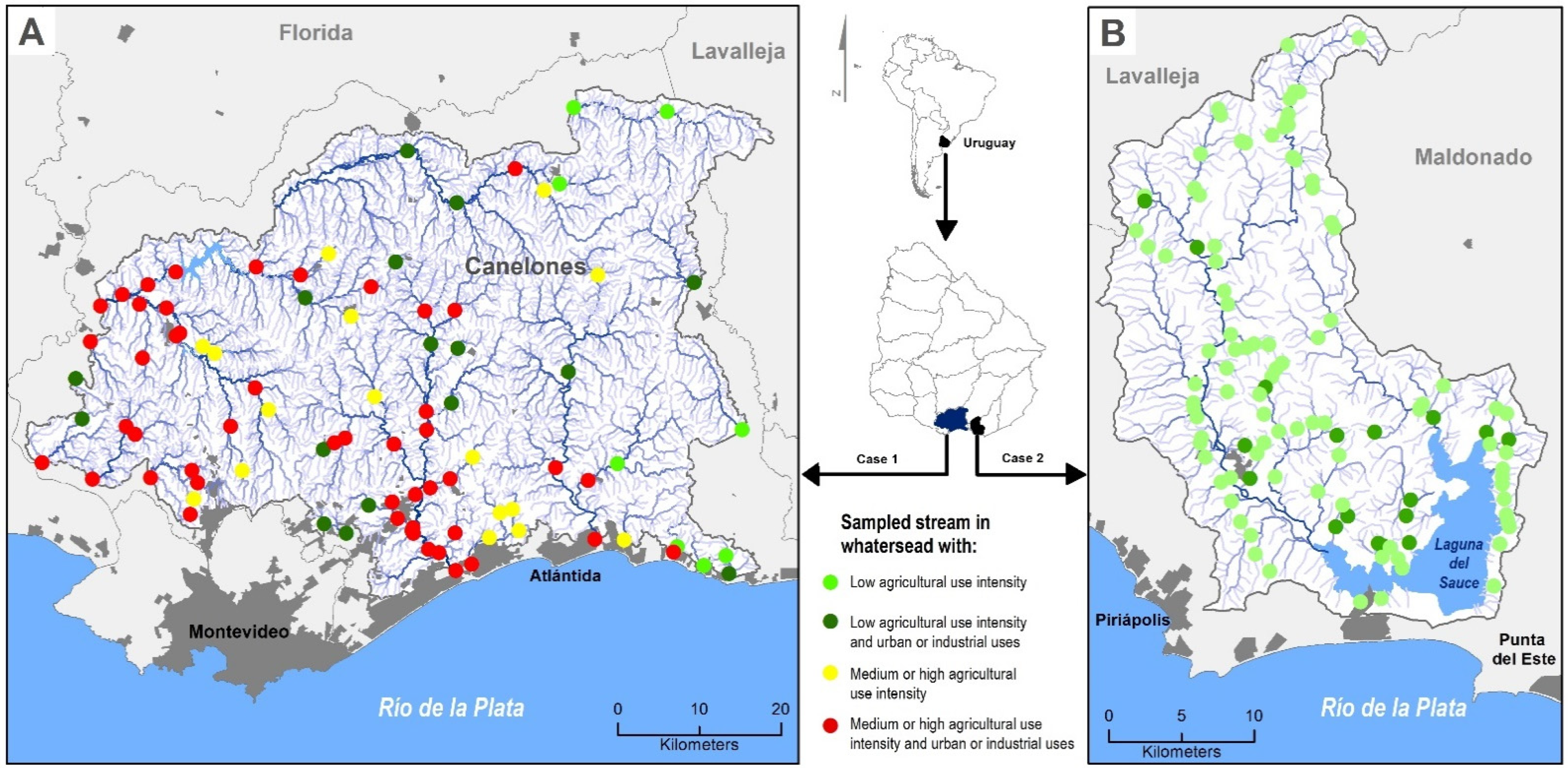
Two case studies were conducted (
Figure 1), as they present contrasting geophysical and land-use characteristics [
47], and are strongly involved in water supply for human consumption. Combined, the area of both case studies provide freshwater for around 70% of Uruguay’s population. The climate in both areas is humid and temperate, with an annual rainfall over 1100 mm and an annual average temperature of 16.4 °C.
Case 1. Located mostly in Canelones and Lavalleja (
Figure 1A) in south Uruguay, has an area of around 349,000 ha, which is subdivided into 87 hydrographic basins (average area: 13,631 ha; minimum area: 200 ha; maximum area: 77,000 ha). Hills are the dominant landform, with slopes under 6%, and the soils are highly fertile [
48]. The most common land uses in rural areas are intensive agriculture and livestock production. This area shows high levels of anthropic soil erosion caused by human production throughout history. The urban population is 250,000 inhabitants, while in rural areas, it is approximately 41,000 [
49]. The majority of towns and cities do not have traditional sewage systems [
50]. In total, 74 agro-industrial complexes were registered, generally located in most densely populated areas.
Case 2. The Laguna del Sauce basin (
Figure 1B) in Maldonado is located southeast Uruguay. It has an area of 70,743 ha, with a broad tributary network. A total of 117 sites were sampled, therefore 117 micro-basins were delineated (average area: 1,558 ha; minimum area: 571 ha; maximum area: 31,107 ha). Most of its surface is covered by natural pasture (53.9%), followed by afforestation (15%). Cattle farming dominates the primary sector activity in the area, with forestry and agriculture in second place. The urban and rural populations are 10,300 and 700 inhabitants, respectively [
49]. Urban development intensification occurs near the water bodies, mainly for residential and touristic purposes.
2.3. Water Quality Data
For Case 1 (Canelones), the water quality data were provided by the Strategic Water Quality Plan for Canelones (PEDCA—IDC [
51]) designed and implemented by the Canelones´ municipality. Two water sampling campaigns were performed in 87 sites. For Case 2 (Laguna del Sauce), data were collected in three consecutive sampling campaigns by Levrini [
52] in 117 sites (
Figure 1). In both cases, data were collected during the WS and SA transitions (2008–2009 in Canelones and 2015–2016 in Laguna del Sauce). The selection of sites aimed to cover the entire study area and account for the diversity of edaphological, geomorphological and land-use conditions, including water systems of social interest, environmentally relevant systems or areas, regions with high pressure on resources, paired micro-basins and location of nonpoint and point sources [
51,
52].
Through using a portable multiparameter sonde, conductivity (K), pH, and dissolved oxygen (DO) data were collected in the field. Water samples were taken below surface in the center of water channel and then filtered with GF/C Whatman. The resulting filters were dried at 100 °C until obtaining constant weight. Afterward, they were heated in a muffle furnace at 500 °C for 15 min and weighed again. The total suspended solids (TSS) concentration and suspended organic matter (SOM) content were estimated by weight difference [
53]. With non-filtered samples, alkalinity was determined through titration with acid according to Wattenberg’s method [
53]. The TP and TN concentrations were estimated from instantaneous-grab sampling using the simultaneous oxidation of phosphorus and nitrogenous compounds with the persulfate of potassium and specific spectrophotometric methods [
54,
55,
56]. Analytic determinations were performed in Centro Regional del Este (UdelaR) the laboratories.
2.4. Land Use and Drainage Basin Characteristics
From the 87 samples corresponding to Case 1 and 117 to Case 2, an equal number of drainage basins were delimited through a digital terrain model (DTM) with 30 × 30 m resolution [
57]. The database source used for modeling started with 13 variables, resulting in 18 parameters (
Table 1). For each basin, a value for each parameter was extracted.
2.5. Data Analysis
The water quality parameters, geophysical attributes, and land use were initially analyzed for each basin using statistical univariate tests. Thereafter, Spearman’s rank correlation coefficient (ρ) was used to identify statistic relationships between these parameters. In the second stage, the existence of spatial dependency between sampling points was analyzed for each temporal period considered by Mantel’s test [
67]. The tests considered the algorithms of Euclidean distance (ED) as the correlation (C) for the physical–chemical and geographical distance for the coordinate matrices. Mantel’s test proved the absence of spatial dependency. Therefore, this aspect was not considered when creating the model. In addition, the spatial patterns for water quality found in both the WS and SA transitions were analyzed using Mantel’s test. In this case, dissimilarity matrices (ED) containing a set of physical–chemical parameters for both periods were correlated. The analysis was performed using R software, version 3.6.1 [
68].
2.6. Modeling
To model the relationship between predictor (land use and watershed geophysical characteristics) and response variables (TP and TN), a Generalized Linear Model (GLM, [
69,
70]) was initially applied. Thereafter, a GAM was used due to could perform better when there are non-linear relationships between variables [
71] (
Supplementary material (SM1)). The water nutrient level is controlled by several natural (i.e., soil type, parental substrate) and anthropogenic drivers (i.e., domestic effluent, agriculture). The GAM allowed us to identify the most important control factors that explain the spatial pattern of the observed water nutrients. One model is generated for PT and another model for NT.
In GAMs, as in GLMs, the components of the Y vector (response variable) are independent variables from an exponential family, this means that the random variables Y1,…, Yn are assumed independent and each Yi has a density function in the linear exponential family (e.g., Normal, Binomial, Poisson, Gamma, etc.)
The predictor and expected values of the response variable Y are related by a link function that must be monotonic and differentiable. GAMs have the following structure:
where g (the link function) is a known monotone differentiable function, μ is the expectation of the response variable, and functions fi(Xi) are smooth functions. These functions are flexible functions that adapt to the data and can be of several forms (cubic splines, natural splines, thin plate regression splines, etc.; for more detail of the construction of the smooth functions we refer to: [
71]). It must be noticed that within one single model, different smooth functions can be considered to model the relation between different predictor variables and the response.
A total of 16 models were generated considering the different areas (Cases 1 and 2), nutrients (TP and TN), periods (WS and SA), and sections of the watershed. The two sections studied to understand nutrient dynamics of drainage basins were: (1) the drainage basin as a whole (section A), and (2) the in-stream processes (section B).
The final set of predictor variables in the models was defined according to Akaike’s Information Criterion (AIC; [
70,
72]) using a stepwise backward selection method [
73]. In this method, the predictor variables are tested in an automatic procedure, and the variables that generate a model with lower AIC are eliminated through a stepped approach. The objective of this method is to reduce the set of variables and choose those that are most important to explain the response variable. With the aim to avoid multicollinearity problems, mainly in GLM models, in cases where the correlation between a pair of variables was greater than 0.5, only one of them was preserved.
The GAMs adjustment was performed using R software [
68], applying the gam function from the mgcv package [
74,
75]. In all cases, the Gaussian family and identity link function were considered, maintaining the other parameters by default. Each model and all variables (response and predictor) used a transformation log (x + 1). This was necessary for the response variables to meet the model assumptions (normal and homoscedastic residue). For the predictor variables, the transformation was used because it significantly improved the model adjustment. The smoot functions thin plate regression spline [
76] was used. The adequate adaptation of the dimension of the smooth functions base according to different predictors was checked using the function gam.check [
74,
75]. The gam.check function test whether the basis dimension (which is related to the degree of smoothness) for a smooth is adequate [
77]. It computes an estimate of the residual variance based on differencing residuals that are near neighbours according to the (numeric) covariates of the smooth. This estimate divided by the residual variance is defined as k-index which is reported by the gam.check function. The further below 1 this is, the more likely it is that there is missed pattern left in the residuals, and then a higher basis dimension is recommended [
77,
78].
The goodness-of-fit measures were evaluated using the adjusted R
2 and Generalized Cross-Validation (GCV, [
79]) values. Both statistics were provided by the gam function. GCV is the model’s mean squared error estimator based on a crossed validation process: the leave-one-out type. Considering that GAMs tend to over-adjust data, the performance measurement was calculated on independent test samples to evaluate its predictive ability. The performance measurement used was the square root of the normalized mean squared error (NRMSE). Its calculation is as follows:
Data were randomly divided into two sets in a 90% training–10% test sampling proportion.
The training sample trained a GAM model with default parameters, and the test sample evaluated model adjustment with the training sample.
NRMSE (evaluation indicator) was calculated as Equation (1):
RMSE refers to the square root of the quadratic error calculated as Equation (2):
where
pred stands for predictor values for trained models on sample test data, and
obs refers to values resulting from the response variable to the sample test.
Lastly, mean (Y) represents the response variable average in the sample test.
In total, 25 random partitions were made, and 25 values for NRMSE were obtained on the sample test. The purpose of doing several splits and averaging results was to avoid bias in NRMSE estimate related to one particular split [
40]. These values were averaged to obtain the NRMSE average (±sd), which indicates the predictive ability of the models. The NRMSE was selected as an indicator due to: (a) it is easily interpretable (values close to zero indicate less residual variance), and (b) it allows easy comparison between models.
2.7. 2030 Scenario
A 2030 scenario was projected based on the assumption of rainfed agriculture (cereals and oleaginous) expansion, and the urban and rural population growth, following the ongoing trend of population growth since 2000 [
63,
78]. Additionally, productive strategies in the area, and urban and industrial source treatment systems were assumed to be constant for the studied period. The database considered for the LCM to project the agricultural and livestock uses for 2030 included the land-use classifications for the years 2000 and 2015, performed using the non-supervised classification of LANDSAT 5TM and LANDSAT 8OLI images and K-means clustering. The approximate area of agricultural and livestock growth was taken from Achkar et al. 2012 [
79] and Uruguay’s Presidential Office of Planning and Budget [
78].
Through the application of the LCM module [
44], the probability of the transition to agricultural or livestock uses was analyzed from a spatial perspective for Cases 1 and 2. The variables under consideration were the soil suitability for agriculture, slopes, road distance, urban areas’ distance, and legal restrictions [
50]. The agricultural and livestock projected areas of growth were distributed according to the detected areas with a greater probability of change. Finally, the values for each basin (sampling point) were integrated with the prediction model for the nutrient concentrations.
4. Discussion
The approach that was carried out allowed the identification of the main drivers of nutrient levels in the water and to predict nitrogen and phosphorus levels in lotic systems. The application of the models under contrasting geophysical and land-use conditions delivered similar results in both cases. Thus, the models developed are a promising tool for applications in different social, economic, ecosystemic, and productive contexts. The tested models allowed the identification of natural and anthropogenic controls for the observed patterns, enabling them to guide the design of strategies and policies to control nonpoint sources, as well as research and action. Applying a predictive model for land-use changes and population growth provided another potential benefit for assessing water quality impacts and land-use planning.
Using GAM models made it possible to explain a substantial part of the spatial variability of TP and TN to a greater extent for both periods and case studies (
Supplementary material (SM3)). GAM models, unlike GLM models, consider different types of relationships (i.e., linear or non-linear) between the response and predictor variables. In addition, the relationships can be of different types for each driver considered. In short, it is an alternative with greater potential if the system is composed of non-linear relationships or different types of relationships between response and predictor variables, a likely situation in study areas with significant environmental and spatial gradients. In addition, the models that included the dissolved oxygen concentration in the water achieved better results in all cases, indicating the importance of considering the internal processes within rivers and streams [
82,
83]. In summary, using GAM models with the combination of landscape attributes and water channel attributes (DO) increased the predictive ability of the nutrient’s models.
A positive association between the contribution of each driver to water runoff (steeper slopes and coarse-grained soils) and nutrient movement was detected [
84]. However, the relationships do not entirely agree with the scientific literature (e.g., slopes and soil type). The spatial pattern of nutrients was conditioned by the spatial distribution of the land-use intensity, where intensive uses—which tend to account for higher TN and TP concentrations in soil—are in areas with favorable geophysical conditions (softer slopes, less degraded soils, fine-grained soils, etc.). On this basis, the land uses possibly mask the influences of the “structural variables”. The sign and the magnitude of the correlation’s coefficient found between the drainage basins’ attributes—geophysical and land use—and nutrient concentrations in both study areas allow us to support this hypothesis. The correlations were significantly stronger in Case 2 (non-intensive land uses) than in Case 1 (intensive land uses). No significant relationships were found for the other drivers (basin size, stream order, and other morphometric and morphologic features).
Geophysical variables should not be interpreted as less important than land-use variables. This implies that if intensive land uses are developed in other geophysical contexts (e.g., soils with stronger slopes, fine-grained and degraded), the nutrient concentrations results would be different, probably higher. For example, reestablishing the intensive production of several areas in Case 1 could unchain an extra input of TP for two reasons: (1) because of the system’s fragility and its predisposition to increased runoff (soil degradation and/or strong slopes), and (2) due to the available TP storage accumulated from previous agricultural uses [
85] in the studied areas’ soils. Some aspects of the models should be highlighted, as that the empirical approaches do not imply that they cannot incorporate causal mechanisms. The strength of empirical models to identify the main drivers of a response variable—as in this work—is simultaneous with their limitations to model behaviors governed by processes that were not identified with a statistical approach. Other approaches, such as deterministic ones, have been successfully implemented in numerous cases (e.g., [
29]) and could contribute to solve some of these problems. Deterministic models offer good results after the calibration of the variables and their application is supported with knowledge of modeling [
86]. However, those models need the parameterization of the variables, which is often expensive, time-consuming and difficult to achieve. A major challenge lies in exploiting the advantages of both models. This would make it possible to understand processes with more precision [
38], improve predictions, and generate a powerful tool to evaluate mitigation measures for specific conditions with no available precedent. This situation would make it possible to resize the role of structural variables. Considering these variables at a lower level of importance than land-use ones, could have serious impacts on water quality. The geophysical and land-use variations between both cases determined clear differences in the waters’ nutrient concentrations and marked distinctions in the models’ attributes. In the Case 1 model, the type of soil variable was not included, but point (industries) and nonpoint sources (rural population) were considered. The rural population density in Case 2 (1.0 hab/km
2) was lower than in Case 1 (11.7 hab/km
2), as well as the point sources, which determined a marginal impact of these actions as sources of limiting nutrients. Finally, the intensity of rural land use in Case 1 was twice that of Case 2, and the production was more diversified [
47], which determined a lower inclusion of the land-use variables in Case 2 (e.g., orchard production).
The projected 2030 scenario would trigger an increase in the nutrient concentrations in water. This increase could intensify the already critical situation detected by the water quality sampling in Case 1, especially for TP. In Case 2, the increases would be lower than in Case 1. However, Laguna del Sauce is an ecosystem that is extremely sensitive to eutrophication (with severe interference to the drinking water supply due to cyanobacterial blooms) given its mean depth and residence time [
87]. Hence, slight changes in land use could lead to a significant intensification of eutrophication.
In Case 1, the increase in the nutrient concentration in water did not correlate with agricultural growth. This pattern is likely to occur because: (i) the intensification of agriculture would be accompanied by an increase in other sources of nutrient export (increase in population and population density), (ii) the pattern of agricultural growth is not homogenous, and covers a large part of the study area, (iii) both factors may hide the role of agriculture as a nonpoint source of nutrients. In addition, the Land Use Planning Ordinance [
50] may control and discourage agricultural expansion and therefore could reduce its impacts on water quality. In fact, the projected scenario already considers a significant area of exclusion for industrial agriculture in the Case 1 (SM 2). Simultaneously, the absence of correlations between the nutrient concentration and agricultural growth detected in Case 1 contributes to new evidence supporting the complexity of the area. We hypothesize that there is a legacy effect of abandoned or replaced agricultural systems and more point sources inputs—from urban and industrial areas—than nonpoint inputs.
In Case 2 (a less complex system showing less intensive land uses and smaller urban and rural populations), agricultural growth was the decisive factor determining an increase in the TP concentrations. An additional phenomenon to be studied is the expansion of afforestation (exotic species) registered in recent decades in Uruguay, a trend that is expected to continue. This variable was not included in generated models. Therefore, it was not included in the 2030 projection either. Since this change in land use would alter the hydrological behavior [
88,
89], it may promote an inferior dilution capacity and, ultimately, increase the risk of eutrophication during drier seasons.
The implemented approach allows for the generation of information for land-use planning at two scales—the drainage basin and region—and for two target resources: water and soil. At a drainage basin scale, it enables the identification of specific land uses in certain locations that may compromise water quality. At a regional scale—a group of micro-basins—it can contribute to the spatial planning design to ensure that changes in rural land use will prevent impacts on water quality. The expansion and intensification of Uruguayan agricultural production have been documented [
90], and the most likely scenario is that this trend will continue. These models are a powerful tool to monitor the impacts of agricultural intensification on the water quality in each basin, a major input for assessing the impacts of land-use changes according to predefined water quality standards/criteria. This information is crucial in rural regions where land-use intensification is imminent (it only remains to decide precisely where), and where national agricultural policies promoting intensification must coexist in harmony with water resource conservation. Incorporating information about changes in agricultural practices into the model (i.e., tillage practice, fertilization and pesticide application methods), and upgrades in treatment systems (urban and industrial), will allow the assessment of different mitigation strategies, a key aspect of water resources management.
In the last two decades, several environmental regulations have been introduced in Uruguay (e.g., Decree Nº405/008—Land Use and Responsible Management Plan [
91]). Nevertheless, the intensification and expansion of agriculture, livestock, and Eucalyptus forestry production [
90] demands new approaches and regulations (especially nutrient input control). The interaction between environmental policies and agrarian intensification raises major uncertainties today. Integrating spatial models elaborated with planning scenarios could improve decision making process. The developed models can provide valuable information for new approaches, such as the construction of projected scenarios [
92] for climate, land-use changes, land-use planning, and environmental policies.
The models developed in this research demonstrate that it is possible to obtain low prediction errors (NRMSE = 15 ± 6) and high correlation between predictive and response values (R2 = 0.53 ± 10) with data from open or available databases, information generated by remote sensing or geoprocessing, and without depending on excessive monitoring efforts after the initial sampling. However, several challenges related to the scaling, updating, and reliability of the data persist and could hinder the implementation of these models in Uruguay. The main challenge is to access up-to-date information generated at manageable costs.
The ability to implement models using currently available secondary information, or easily collected at a low cost, is the most remarkable feature of this approach. The generated models are a viable alternative for expanding our knowledge of ungauged Uruguayan aquatic systems.
5. Final Remarks
The combination of different approaches—GIS, GAM, RS, and LCM—shows that it is possible to develop efficient local spatial models, with a moderate data collection effort, to evaluate the nutrient concentration in lotic systems.
The developed models show the importance of land uses as the main drivers of nutrient concentration in the water, as well as the contribution of natural (structural) control factors. In addition, the models made it possible to determine the role of the key internal processes of the aquatic ecosystems, such as the dynamic of oxygen concentration, on a nutrient level.
The results suggest that for long-term solutions to water quality problems, it is essential create productive systems with nutrient balances close to zero or, in the most critical situations, negative. Similarly, there is still a need to improve the point source control and sewage system efficiency. Actions focused on the final phase of the nutrient export process—to implement buffer areas—could contribute to the reduction of nutrient input into water ecosystems. However, these actions will not be fully sufficient if the processes associated with agriculture in upper and medium drainage basins are not monitored and controlled.


 ,
, 


