Model of Predictive Maintenance of Machines and Equipment

Abstract

This paper presents selected possibilities for mathematical models in predictive maintenance of equipment. This model includes automatic classification of machines by labor intensity, determination of labor intensity standards, and drawing up monthly and yearly maintenance plans for manufacturing lines and technical equipment in an engineering company. This model reduces human error, clarifies accounting and operational records of machines, evaluates the actual maintenance labor intensity, eliminates routine administrative work, enables the use of cloud storages, and includes automatic reporting of problems in the case of on-board diagnostic systems. It is based on differentiated machine care, can be an effective tool for the overall optimization of maintenance processes, and is a part of the digitization of these processes in engineering companies.

1. Introduction

Industry 4.0 (also the Fourth Industrial Revolution), or Maintenance 4.0, is an indication of the current trend of digitization, the associated automation of production, and the changes in the labor market induced by these processes. Its implementation involves the use of machine perception methods, self-configuration, and self-diagnostics with computer connected equipment, parts, and control and logistics processes, including maintenance. The products and machines are equipped with chips, for control and operation over the Internet. In addition, cloud storage, 3D printing, data centers, automated reporting of problems, “smart maintenance”, or “smart warehouses” will be used to inform about depleted stocks, etc. A partial contribution to this trend is keeping the operability of production machines and equipment, which are the basic means of fulfilling the Industry 4.0 concept. Quite a large number of maintenance optimization solutions, according to different criteria, exist in practice. Some modern solutions are listed in [1,2,3,4,5,6,7,8] and others. Most companies follow the maintenance program (maintenance regulations), which determines at what intervals and to what extent the equipment undergoes individual maintenance stages (inspection, preventive, predictive and proactive maintenance, revisions, diagnostic repairs, and overhauls, etc.). The intervals are determined by the machine manufacturer’s recommendations, experience, legislation, optimization calculations from failure statistics, etc. Standard optimization methods include RCM (Reliability Centered Maintenance), which reduces cost and ensures greater safety and availability. The RBI (Risk Based Inspection) method optimizes inspection and maintenance activities, and focuses mainly on information about possible leakage of the working or lubricating medium of the machine (American Petroleum Institute Recommended Practice 580—API RP 580). Additionally, the SIF (Safety Instrumented Function) method is used to optimize test intervals for protection devices, alarms, etc. The IMS (Integrated Maintenance Solutions) method is an alternative to in-house maintenance practice or full outsourcing and subcontracting, and includes continuous monitoring, analysis of results, and real improvement of maintenance. The general method for optimizing the maintenance is based on cost and lifetime information. The information base for these solutions is the analysis of diagnostic measurements aimed at determining the optimal values of diagnostic signals, so-called “standards” for maintenance (renewal) purposes. Standard stochastic methods are used to determine the values of diagnostic signals that require maintenance or renewal of the machine. The authors based the mathematical model on the facts reported in [9,10], and used the programs in [11,12,13]. The presented model utilized real data from the workshop of an engineering company that specialized in the manufacture and repair of special military equipment. The operability of machines and equipment was arranged in terms of time perspective, but mainly in a factual perspective (maintenance, inspection, overhaul, renewal). From this point of view, it is a two-dimensional matrix with one edge focused on the factual perspective and the other on the time perspective. The standard-setting process also plays an important role; it expresses the maintenance labor intensity using differentiation according to the importance of the machine, structural complexity, repair characteristics, weight, accuracy, etc. A graphic showing the creation of the standard is expressed by the algorithm is in Figure 1.

Maintenance planning is a relatively complicated issue that can be addressed using modular software tools that are currently commercially available [13,14,15]. The software [16] was used as the authoring solution; it models maintenance and contains the following basic modules:

• determining the basic level of maintenance labor intensity,
• creating the maintenance labor intensity standard,
• creating an operational maintenance plan according to the specificity of the business.

To solve this issue, an information system [17,18] is required, that includes the following specific information:

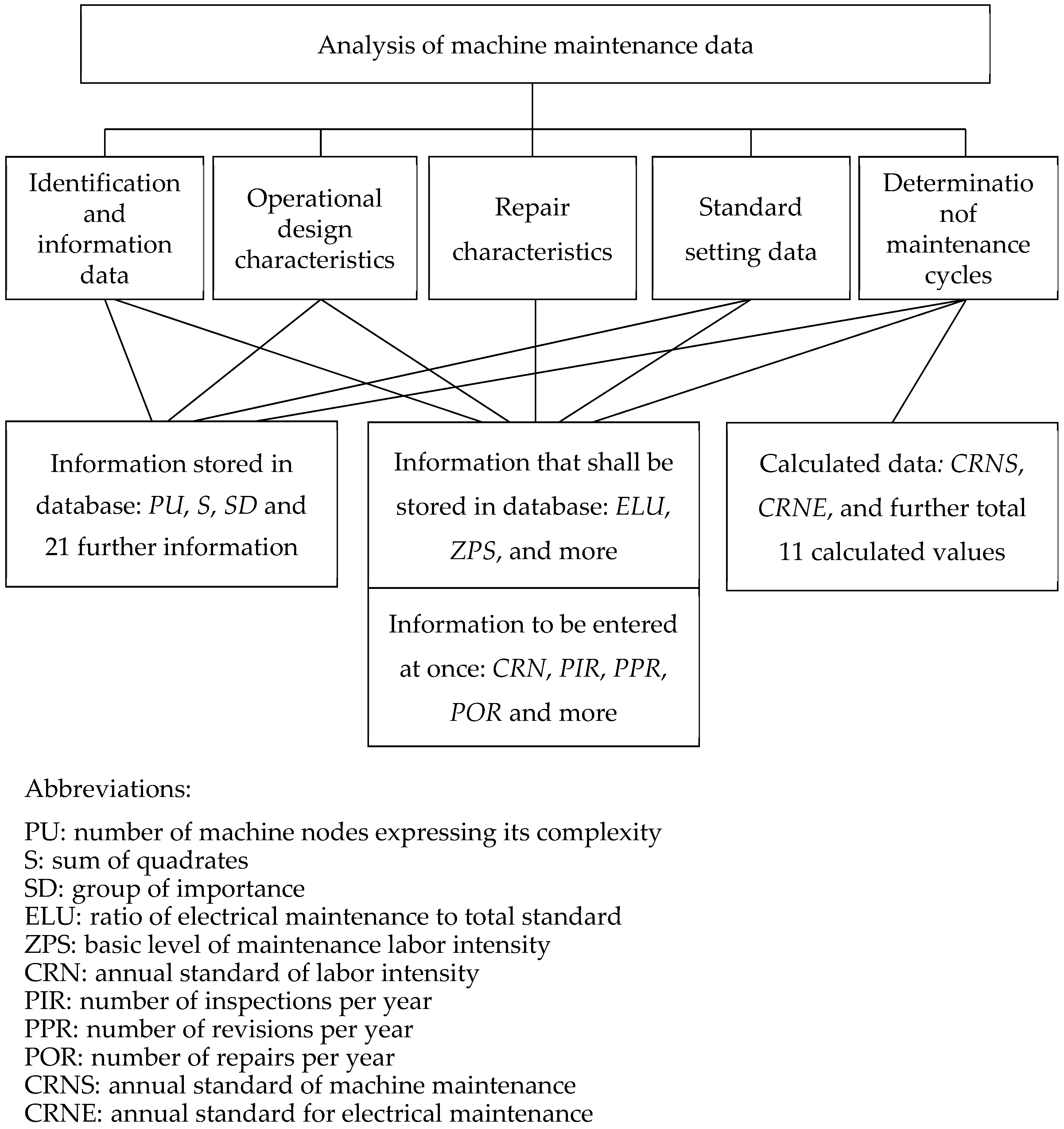
• identification of the essential means,
• design and operation characteristics,
• reliability and maintenance characteristics,
• data to determine the maintenance standard,
• data to determine the maintenance cycle/periodicity (capacity, spare parts, equipment, etc.).

The analysis of the data used to optimize machine maintenance is shown in Figure 2.

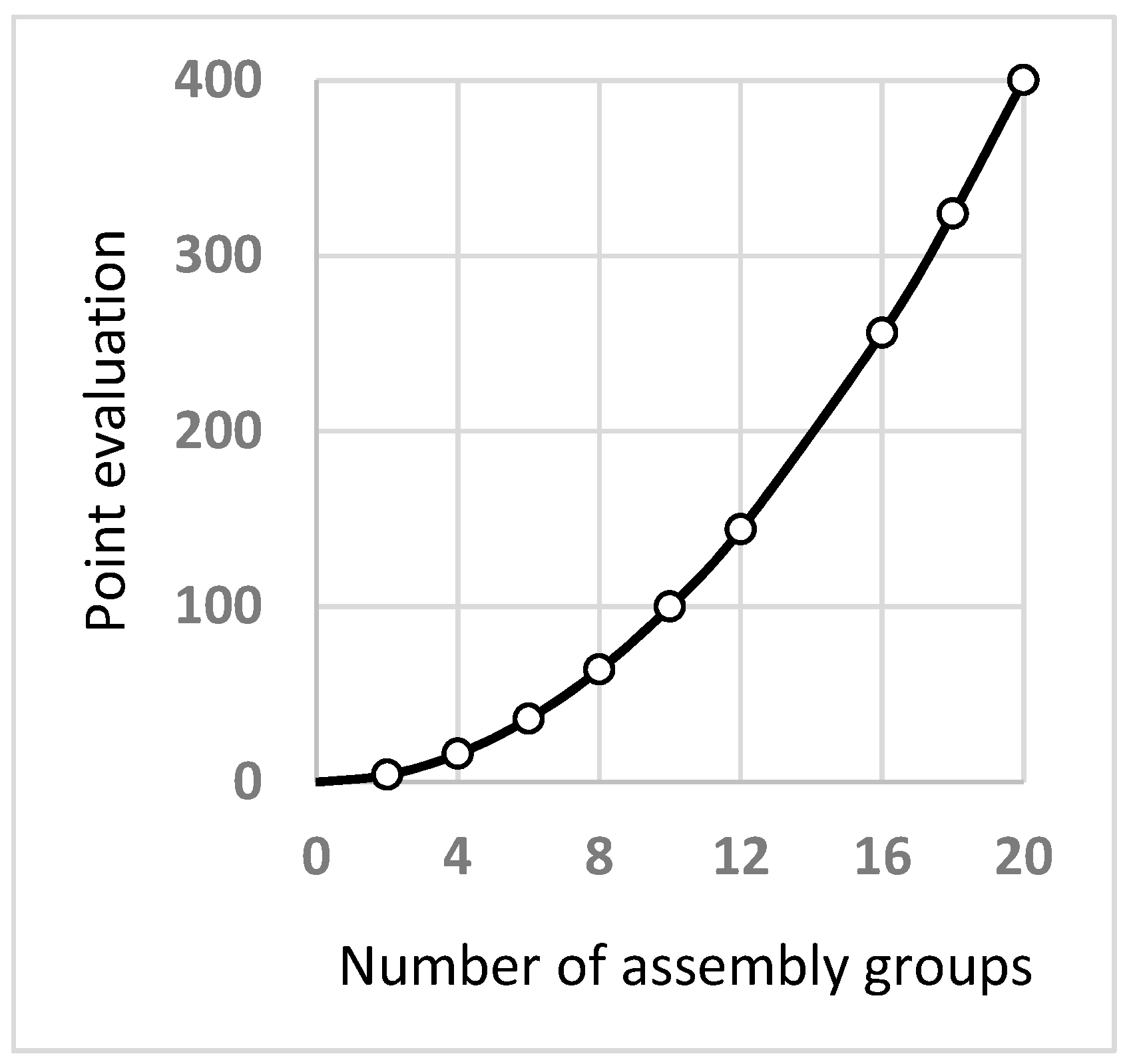
2. Model of Basic Level of Labor Intensity

The basic level of labor intensity is based on expert point evaluation of: machine complexity (number of assembly groups); technical level i.e., the degree of automation (mechanical, semi-automatic, fully automatic); accuracy (standard, accurate, very accurate, extremely accurate); and weight (kilograms or tons). The criterion for classifying the machine by labor intensity is the sum of the points [9,17,18,19,20]. The dependence of the number of points $P$ on the machine parameter $p$ is given by

$$P =f\left(p\right)$$

(1)

The number of points $P$ is determined for each parameter $P$ by another function, and the sum of the points ${\displaystyle \sum }P$ is then the parameter of the function of the basic level of labor intensity $Z$, when

$$Z =g\left({\displaystyle \sum }P\right)$$

(2)

The dependence of the number of points on the parameters of a particular machine can be expressed graphically for two variants of the solution, taking into account the specific limitation of the solution [21]. In this case only four basic mathematical operations were used. The graphical representation of the dependence of the number of points on the number of assembly groups is a parabola (this dependency expresses the complexity of the machine), shown in Figure 3, and the number of $P_1$ equals

$$P_1=p_1^2$$

(3)

The graphical representation of the dependence of the number of points on the machine accuracy, shown in Figure 4, is a straight line or

$$P_2=p_2$$

(4)

The dependence of the sum of the assigned Z points on the weight, technical level, and basic level of preventive maintenance can be approximated in several ways. Two methods were chosen based on the results of the test data set: rational fractional function (point 1) and polynomial (point 2).

Ad point (1)

Rational fractional function

$$Y =\frac{A +BX}{C +DX}$$

(5)

where A, B, C, and D—function coefficients; $X$—parameter; and $Y$—number of points.

To approximate Equation (5), we use:

(a) Coordinate optimization leading to the minimizing or maximizing task.

The values of the coefficients A to D are searched, so that the sum of the squared deviations $S ={\displaystyle \sum }{(Y-Y_i)}^2$ between the entered value of $Y_i$ and the calculated value of $Y$ at the point $X_i$ is minimal. The initial values of the coefficients are chosen so that the rational fractional function passes through the endpoints and the selected midpoint, thus determining the three coefficients A, B, and C, and choosing the fourth one arbitrarily with the condition that $D>1$ (Figure 5). After substituting the selected points and adjusting, we get the following set of linear equations:

$$\begin{gathered} A +B{X}_1-C{Y}_1=D{X}_1{Y}_1 \\ A +B{X}_3-C{Y}_3=D{X}_3{Y}_3 \\ A +B{X}_6-C{Y}_6=D{X}_6{Y}_6 \end{gathered}$$

(6)

To solve this system, we use the Gauss elimination method. The equations are adjusted to the form (Equation (7)), we choose the difference value $\Delta$, by which we gradually change the size of the coefficients [22]. We calculate the sum of variances $S$, and for $S_{min}$ we adjust the coefficient to the next calculation step. We terminate the iteration when the sum of the variances can no longer be reduced or after performing a predetermined number of iterations.

$$\left[\begin{array}{c}1\\ 1\\ 1\end{array}\begin{array}{c}{X}_1-Y_1\\ X_3-Y_3\\ X_6-Y_6\end{array}\right]·\left[\begin{array}{c}A\\ B\\ C\end{array}\right]=D\left[\begin{array}{c}{X}_1{Y}_1\\ X_3{Y}_3\\ X_6{Y}_6\end{array}\right].$$

(7)

(b) Least squares method

This method uses Equation (5) to determine the relationship between the X and Y variables by using an iterative algorithm. We constructed a Jacobi matrix, whose elements form partial derivatives of the approximation function (Equation (8)).

$$\begin{gathered} \begin{array}{cc}\frac{\partial Y}{\partial A}=\frac{1}{C +DX}& \frac{\partial Y}{\partial B}=\frac{1}{C +DX}\end{array} \\ \begin{array}{cc}\frac{\partial Y}{\partial C}=\frac{A +BX}{{(C +DX)}^2}& \frac{\partial X}{\partial C}=\frac{X\left(A +BX\right)}{\left(C +DX\right)}\end{array} \end{gathered}$$

(8)

We determined the corrections using the residue $R_i=Y =Y_i$, where $Y_i$ is the entered value corresponding to coordinate $X_i$. Partial derivatives of the approximation equation of scalar products are solved by the Gauss elimination method. In each subsequent iteration step, we determine new values of the coefficients A, B, C, and D, by adding corrections to the value from the previous iteration $A^{k+1}=A^k+A$, etc. We terminate the iteration when the sum of the squares of deviations ${\displaystyle \sum }{(R_i)}^2$ reaches the required accuracy, or when we perform a predetermined number of iterations [16,23,24], etc.

Ad point (2)

Generic n-th polynomial

$$Y =A_0+A_{1}X +\cdots A_{n-1}{X}^{n-1}+A_n{X}^n.$$

(9)

It is solved by the method of perpendiculars from point to linear half-space. In the first phase, we define the matrix of base vectors $D \left[15, N\right]$ and assign $K = 2$, which corresponds to the number of coefficients in the first degree polynomial

$$\begin{array}{cccccc}\hfill 1\hfill & \hfill 1\hfill & \hfill 1\hfill & \hfill \cdots \hfill & \hfill 1\hfill & \hfill 1\hfill \\ \hfill X_1\hfill & \hfill X_2\hfill & \hfill X_3\hfill & \hfill \cdots \hfill & \hfill X_{N-1}\hfill & \hfill X_N\hfill \\ \hfill X_1^2\hfill & \hfill X_2^2\hfill & \hfill X_3^2\hfill & \hfill \cdots \hfill & \hfill X_{N-1}^2\hfill & \hfill X_N^2\hfill \\ \hfill X_1^3\hfill & \hfill X_2^3\hfill & \hfill X_3^3\hfill & \hfill \cdots \hfill & \hfill X_{N-1}^3\hfill & \hfill X_N^3\hfill \\ \hfill ⋮\hfill & \hfill ⋮\hfill & \hfill ⋮\hfill & \hfill \cdots \hfill & \hfill ⋮\hfill & \hfill ⋮\hfill \end{array}$$

We calculate from the matrix $A\left[K,K +1\right]$, whose elements we mark

$${{\displaystyle \sum }}_{j=1}^K\left(D_j·D_i\right)·a_j=Y·D_i i =1,2,\dots K$$

(10)

where $\left(D_j·D_i\right)—$ scalar product of rows of the $D$ matrix, $a_j$—coefficients of the approximation polynomial, $Y·D_i$—the scalar product of the vectors specified by Y coordinates and the row of the D matrix.

Calculation of the basic level of operational maintenance from the product of technical parameters points is based on [12]. For approximation by rational fractional function, we proceed according to the following algorithm:

• enter values A, B, C, and D for the technical level of the machine, its weight, and the basic level of accuracy;
• enter the characteristics of the number of groups, technical level, weight, and level of accuracy;
• we gradually calculate the number of points for each characteristic, and we determine the basic level of maintenance from their sum.

Note: For polynomial approximation, the algorithm is the same; only instead of the coefficients of a rational fractional function, enter the degree of the polynomial and its coefficients in the order of the absolute member to the highest power.

The graphical evaluation of the results obtained by the approximation is shown in Figure 6, Figure 7 and Figure 8. The results show the deviations of the individual functions from the given points [22]. Numerical evaluation is given in

Table 1. Evaluation of the approximation of technical level of machines.

Parameter X	Entered Values	Deviations of Approximated Functions
		Least Squares Method	Coordinate Method	Polynomial Method
1	1	10.31	6.11	−0.19
2	5	5.68	0.55	0.17
3	10	0.21	−7.78	1.03
4	20	−2.73	−9.40	−0.95
5	40	0.83	−6.10	−3.24
6	80	19.30	12.94	6.53
7	100	9.77	5.91	−4.40
8	125	−8.01	−5.39	1.05
	Dispersion	83.86	53.48	9.46

,

Table 2. Evaluation of machine weight approximation.

Parameter X	Entered Values	Deviations of Approximated Functions
		Least Squares Method	Coordinate Method	Polynomial Method
1	1	0.05	−0.94	−0.78
2	4	1.08	0.07	−0.15
3	6	1.16	0.14	−0.15
4	8	2.29	0.27	−0.19
5	10	1.49	0.45	−0.13
6	12	1.72	0.61	0.001
7	14	2.00	0.97	0.22
8	16	2.33	1.30	0.51
9	18	2.50	1.68	0.87
10	20	3.12	2.09	0.87
11	21	2.58	1.45	0.78
12	22	2.07	1.06	0.32
13	23	1.61	0.59	−0.09
14	24	1.18	0.17	−0.45
15	25	0.78	−0.22	−0.76
20	30	−0.72	−1.66	−1.73
30	40	−1.71	−2.52	−1.32
40	50	−0.65	−1.29	1.38
50	55	−3.06	−3.54	0.65
60	60	−4.31	−4.62	0.55
70	65	−4.65	−4.80	−0.21
80	70	−4.26	−4.21	−2.79
90	85	6.72	6.84	2.78
100	90	8.18	8.43	−0.76
	Dispersion	9.79	9.12	1.19

,

Table 3. Evaluation of approximation of basic level of maintenance labor intensity.

Basic Level of Maintenance	Entered Values	Deviations of Approximated Functions
		Least Squares Method	Coordinate Method	Polynomial Method
1	4–6	−0.9–4.2	−1.0–4.4	2.5–9.5
2	6–8	4.5–10.8	4.4–19.9	17.0–26.0
3	8–15	10.8–18.4	10.9–18.6	17.0–26.0
4	16–25	18.4–27.5	18.6–28.0	26.0–36.5
5	26–40	27.5–38.9	28.0–39.5	36.5–50.2
6	41–60	38.9–53.3	39.5–54.2	50.2–70.0
7	61–83	53.3–72.1	54.2–73.7	70.0–100.0
8	84–105	72.1–97.9	73.7 -99.6	100.0–150.5
9	106–135	97.9–135.2	99.6–137.5	150.5–212.0
10	136–245	135.2–194.2	137.5–197.3	212.0–308.0
11	246–330	194.2–301.3	197.3–305.5	308.0–387.5
12	331–400	301.3–555.9	305.5–560.0	387.5–409.3
13	401 and next	555.9–1982	560.0–1906	409.3–423.2
	Dispersion	$2.33\times {10}^3$	$2.41\times {10}^3$	$3.22\times {10}^3$

,

Table 4. Values entered to validate the mathematical model.

No.	Number of Groups	Degree of Accuracy	Technical Level	Weight in t	Manual Sum of	Processing $\mathit{B}\mathit{L}\mathit{P}\mathit{M}$
1	1	1	3	2	24	4
2	4	4	2	4	33	5
3	5	2	4	5	57	6
4	6	11	3	7	71	7
5	7	6	4	10	95	8
6	8	12	4	15	121	9
7	9	9	5	50	185	10
8	10	50	7	30	290	11
9	15	11	6	40	366	12
10	18	80	7	100	594	13

and

Table 5. Analysis of results achieved by different methods.

Serial Number	Sum Deviations			Sum Deviations
	Least Squares Method	Coordinate Method	Polynomial Method	Least Squares Method	Coordinate Method	Polynomial Method
1	−1.3	5.7	−1.0	0.0	1.0	0.0
2	−7.0	−0.8	0.0	−1.0	0.0	0.0
3	1.2	7.9	1.0	1.0	1.0	1.0
4	−2.2	4.8	−1.2	0.0	0.0	0.0
5	−0.4	7.3	−0.4	0.0	0.0	0.0
6	1.9	9.6	1.7	0.0	0.0	0.0
7	2.3	9.6	2.5	0.0	0.0	0.0
8	−8.1	−3.4	5.7	0.0	1.0	0.0
9	−18.6	−11.7	−7.9	0.0	0.0	−1.0
10	−18.0	−14.3	5.3	0.0	0.0	95
Dispersion	80.2	70.9	13.6	0.2	0.3	902.7

. It follows that the smallest deviations from the given points can be identified in the polynomial approximation. We use the fourth degree polynomial for the dependence of the point evaluation of the degree of automation. We use the sixth degree polynomial for the dependence of point evaluation on weight. To calculate the basic level of maintenance labor intensity, we use a rational fractional function, whose coefficients are determined by the least squares method.

Best modelling results achieved:

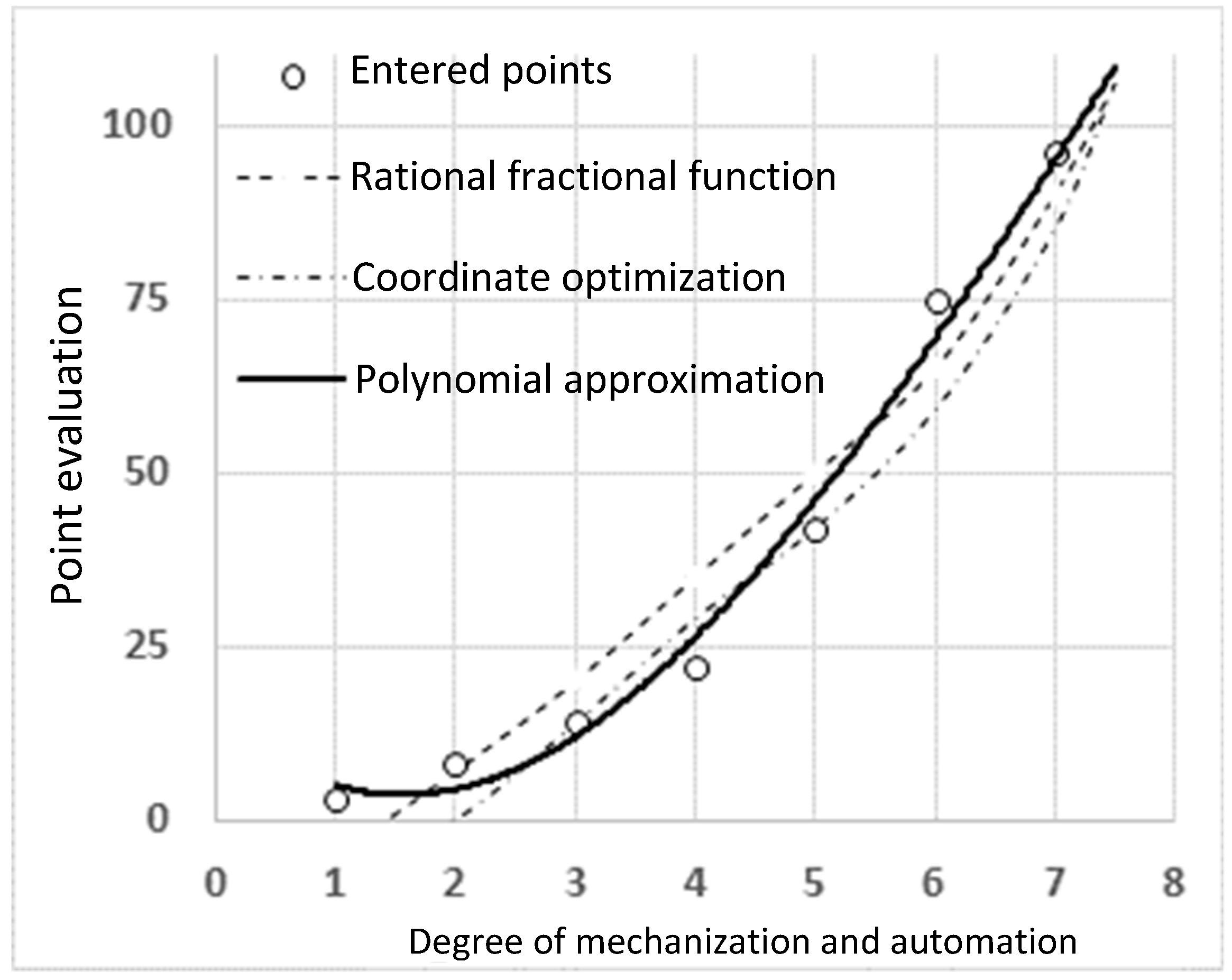
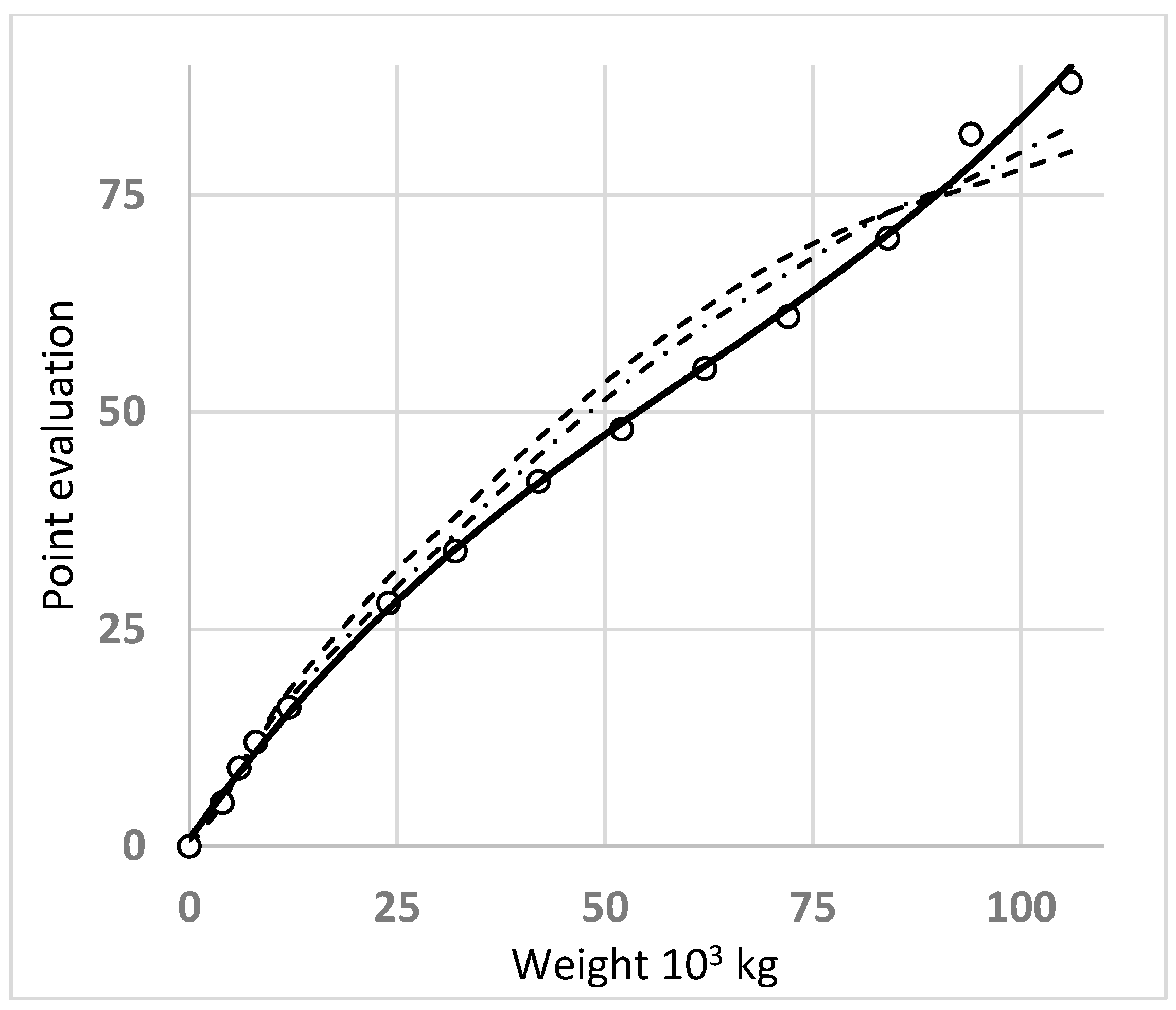
• for the sum of points, the model using the polynomial;
• for the basic level of operational maintenance, the model using a rational fractional function;
• for coefficients, the model using the least squares method.

These results confirm the possibility of using the three above mentioned functions for the mathematical model of calculating the basic level of maintenance, directly from the design and operational parameters of the machine [14,25].

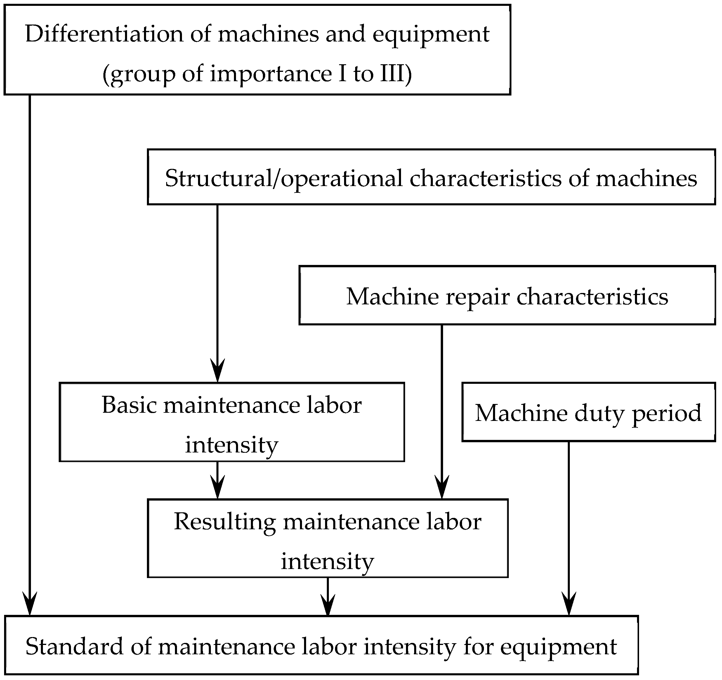
3. Mathematical Model of Maintenance Standard

The objective of the model is to determine the number and type of maintenance interventions, including the number of hours required to perform maintenance on the machine or equipment, for a calendar year [15]. The flow chart of the program for standard assignment is shown in Figure 9. The model algorithm is based on:

• Calculation of the basic level of labor intensity is based on:
  • machine complexity: $B_1=PU·PU$;
  • technical level: $B_2=A +B·S +C·S^2+D·S^3+E·{\mathrm{S}}^4$;
  • weight: $B_3=A +B·MW +C·M{W}^2+D·M{W}^3+D·M{W}^4+F·M{W}^5+G·\mathrm{M}{W}^6$;
  • machine accuracy: $B_4=PRN$;
  • total points: $SB =B_1+B_2+B_3+B_4$.
  The basic level of labor intensity is then

  $$ZPS =\frac{A{}^{″}+B{}^{″}·SB}{C{}^{″}+D{}^{″}·SB}.$$

  (11)
• Calculation of final degree of labor intensity is

  $$K =ZPS +OPC.$$

  (12)
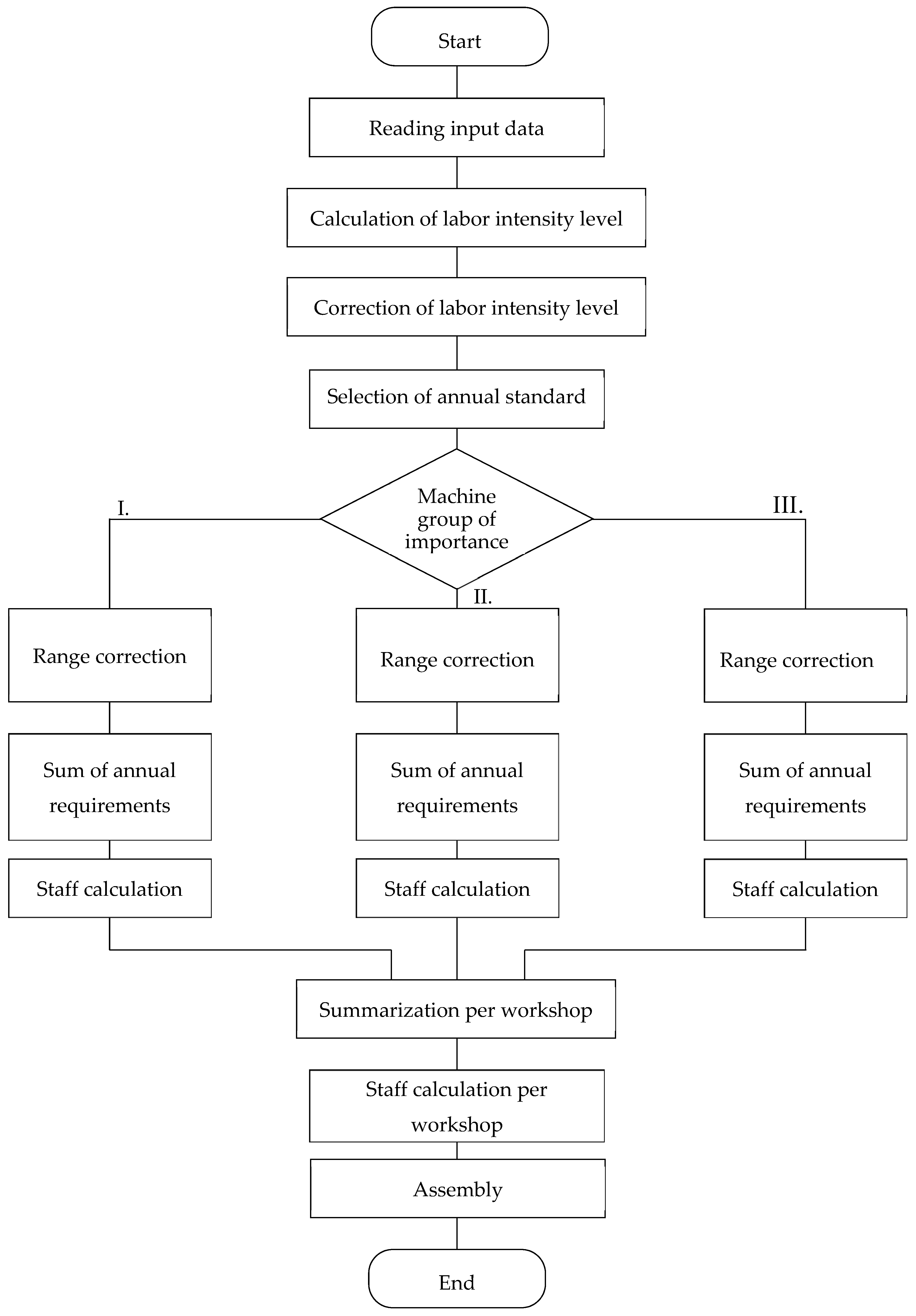
• In the standards, find the number, type, and extent of maintenance operations for each machine according to $A\left(SD,ZU,K\right)$.
  Note: The standard contains information on the annual norm of labor intensity in hours, number of inspections per year, extent of one inspection in hours, number of repairs per year, and the extent of one repair in hours.
• Breakdown of annual standard of labor intensity for:
  • electrical maintenance: $CRNE =\frac{ELU}{100}·CRN$,
  • machine maintenance: $CRNS =CRN-CRNE$.
• Maintenance staffing calculation
  • total hours of annual standard: $C ={\displaystyle \sum }_{i=1}^{n}CR{N}_i$
  • total hours of machine maintenance: $S ={\displaystyle \sum }_{i=1}^{n}CRN{S}_i$
  • total hours of electric maintenance: $E ={\displaystyle \sum }_{i=1}^{n}CRN{E}_i$
  • staffing total: $KPCS =\frac{1.2·C}{ED}$

Note: The value 1.2 in the above mentioned relation means that 20% is added to the total annual C standard as a reserve.

4. Model of Operational Maintenance Plan

Calculations for machines and labor force efficient pool are:

• annual effective pool of the machine: $E_S=\left(260-d_d\right)·\left(1-\frac{{\eta }_3}{100}\right)·f_d$.
• annual pool of one worker: $E_D=\left(260-d_d\right)·\left(1-\frac{{\eta }_1+{\eta }_2}{100}\right)·f_d$.

The algorithm of the annual maintenance plan contains:

(a)

Basic information or possible changes:

• machine importance group,
• way of use (shifts),
• repair characteristics,
• date of last repair,
• machine utilization in %,
• percentage of machine maintenance and electrical maintenance.

(b)

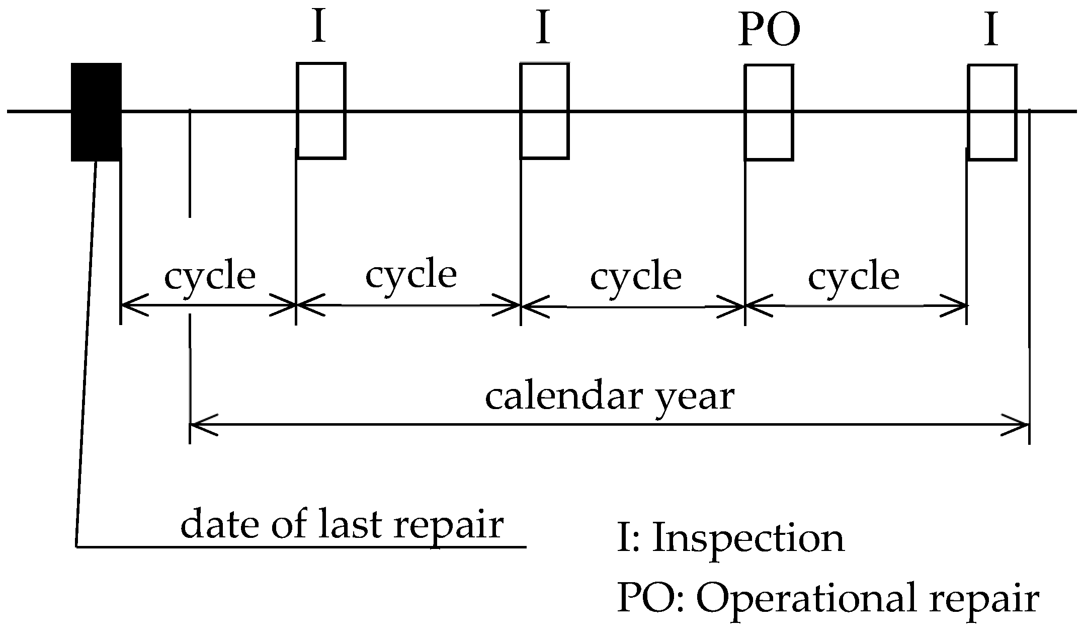
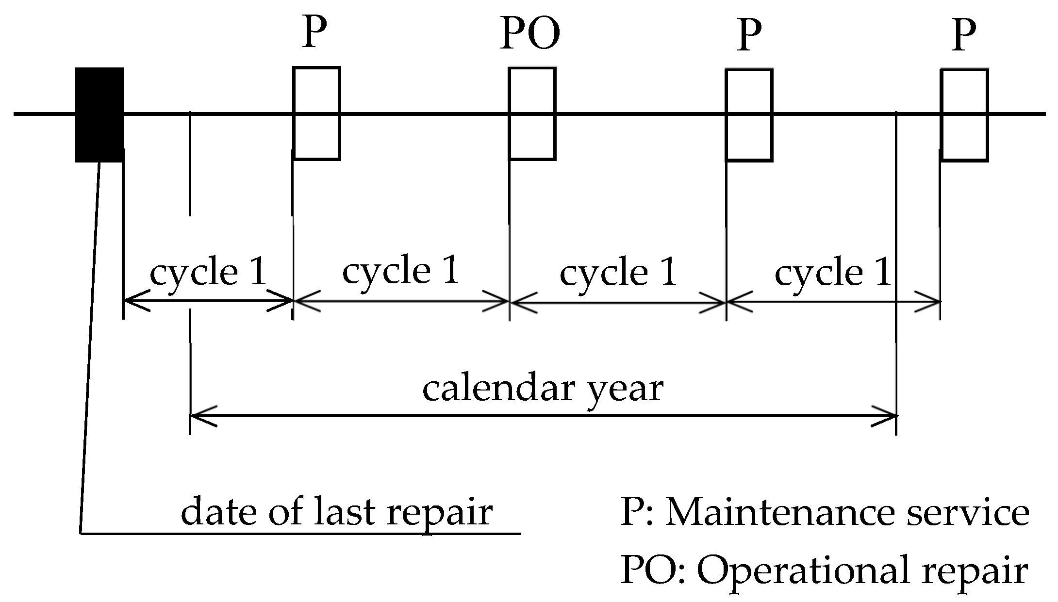
Calculation of cycles (time between maintenance operations for machine importance groups I, II, and III).

(c)

Division of maintenance tasks into time series.

(d)

Symmetrical distribution of maintenance tasks, respecting the capacity limitation of maintenance staff, and the use and importance of the machine.

• Calculation of cycles, i.e., periodicity between maintenance activities for:
  • Group of importance I: $=\frac{E_S}{PIR +PPR +POR}$.
  • Groups of importance II and III: $=\frac{E_{S\left(2-\frac{PVS}{100}\right)}}{PIR +PPR +POR}$.
  Note: The group of importance I are unique machines, group II are standard machines, and group III are auxiliary machines and equipment.
• Distribution of activities into a time series for:
  Group of importance (Figure 10):
  Group of importance II and III (Figure 11):
• Symmetrical distribution of maintenance operations with reduced utilization of workers’ capacity, taking into account the importance group of the machines.

5. Discussion

The presented text consists only of selected information from a very extensive project on maintenance optimization, and accurate records of machines and equipment in the selected company. It was a long-term project which can be schematically divided into four stages. The first stage is characterized by an analysis of implementation options, database creation, user programs, diagnostic programs and outputs, management, and maintenance staff training. The second phase involved data collection and coordination of specialists (data analysts). The input data was arranged as sequential files (indexed, tree-hierarchical, and networked). The maintenance data files contained maintenance objects, drawings, stored spare parts and supplies, type standards of work, etc. The third phase was the process of pilot data analysis. The fourth phase included project implementation, compilation of outputs and analyses, integration into the existing information system, and updating in case of changes and for practical use.

Simple models such as second degree planar curves, rational polynomial function, general polynomial, etc., were used to move from heuristics-based approaches to maintenance, based on calculations from both current and historical data. The main problems of the solution were the differentiation of machines and equipment according to their importance in the production process, inclusion in the appropriate level of maintenance labor intensity (13 levels in total), determination of machine shifts, and standards of annual repair activities. The parameters were objectified on the basis of the created knowledge-based system, knowledge base using forward chaining based on data-driven reasoning (creation of a modular knowledge base including heuristics and exact knowledge), the inference mechanism, interface, explanatory module, and the knowledge acquisition module. It can be stated that the maintenance of machines and their efficiency was massively conditioned by the processing of maintenance data, database platform (Firebird, MySQL, MS SQL, Oracle, etc.), performance of the hardware, actual maintenance, and proper use of standardized query language SQL (Structured Query Language). Specifically, the optimization meant finding the optimum time between maintenance interventions, individual determination of the maintenance content based on real-time information about the technical condition, and refining the maintenance work technology for a particular machine. After introducing the new maintenance system, it is rightfully expected to improve maintenance planning, cost-effectiveness, and other intangible benefits. According to various literary sources, time after implementation could possibly be reduced by up to 30% [20,23]; specific information from the pilot project was only from one workshop (mechanical machining workshop) from the company where the project was implanted and is 7%, as shown below.

Along with the current complexity, extent, automation, and concentration of production machines, the probability of failure increases inevitably. Complexity (number of elements) and extent (number of systems: control, regulation, electronic, mechatronic, electrical, mechanical, hydraulic, pneumatic, etc.) depend on their specific connection (serial, parallel, combined) and degree of automation (without automation elements, using the operator = hands on, partial automation = hands off, conditional automation = eyes off, high automation = mind off, complete auto-automation, mechanical or software robotization of the machine). As for the concentration of machines, this relates to the number of different machines that have different maintenance requirements (in terms of the number and complexity of operations, maintenance staff qualifications, maintenance time, etc.). The number of elements of a particular machine is decisive, as far as the number of possible failures is concerned. The current maintenance of machines and equipment during the period of use is gradually expanding to the conceptual preparation stages; the main reason is connected with the sustainability of related decisions by the designers and engineers. The basic goal of the whole maintenance system is then to ensure good machine availability, which is a characteristic, measurable parameter; the standard value should be higher than 0.95, which is a sign of good use of the equipment (machine work intensity) and its age. The novelty of the considered approach consists of a completely individual evaluation of the machine in terms of maintenance requirements (content, scope and periodicity) by means of a combined system (real-time diagnostics of the main groups of the machine and the submitted author’s model). The presented model can be considered objective because it is based on three basic principles, namely:

• Determination of the absolute values of indicators used (external-knowledge system, determination of variables based on user experience and recommendations of manufacturers, finding the range of indicator values based on maximizing the probability of trouble-free operation by the calculation and verification using statistical surveys from the existing representative, valid, and reliable data).
• Determination of relative values of used indicators (size of relative intervals, determination of standard indicators, dependence between relative and absolute indicators, compensation of impermissible values of indicators, application of time factor in evaluation).
• Determination of values of complex indicators (weighting coefficients according to experts, scales with individual division according to machine characteristics, errors in determination).

A separate area of the solution is the issue of human errors in the human-machine systems, which are a risk in every profession, including maintenance. In the project, the following measures were respected: partial changes in technological procedures and maintenance organization (replacement of human intervention with modern means of dismantling and assembly, removal of ambiguities and incomprehensible instructions in working procedures, personalized responsibility of specific employees for the entrusted activity, time consuming work), material and technical maintenance (passive safety elements, lighting, movable element covers), and partial changes in the field of maintenance staff (regular training and checking, feedback from maintenance personnel in critical positions).

6. Conclusions

The created mathematical model for the predicative maintenance of the basic equipment (machines) is based on the calculation of the basic level of operational maintenance, labor intensity standards of machines, and the creation of the algorithm for the operational maintenance plan. The verification was carried out through the creation of an annual operating maintenance plan; and its evaluation, by a workshop of a real engineering company engaged in the production and repair of special vehicles. A Passport of each machine is the concrete result of the model; it contains basic record-keeping information for efficient operation and maintenance. The Passport of the machine uses an information system based on a relational database with a classic two-dimensional structure; the processed software can present this information in real time. Results of the previous partial search showed massive improvement of information on planned and actual maintenance activities (automatic document generation), a rise in efficiency in the care of machines and equipment (from available partial data financially expressed by 7%), and better utilization of maintenance staff (data not available yet or not public). The model and its implementation is the first step in the optimization and digitization of maintenance processes.

References

1. Knopik, L.; Migawa, K. Multi-State Model of Maintenance Policy. Maint. Reliab. 2018, 20, 125–130. [Google Scholar] [CrossRef]
2. Valis, D.; Pietrucha-Urbanik, K. Utilization of Diffusion Processes and Fuzzy Logic for Vulnerability Assessment. Eksploat. Niezawodn. Maint. Reliab. 2014, 16, 48–55. [Google Scholar]
3. Diaz, N.; Pascual, R.; Ruggeri, F.; Droguett, E.L. Modeling Age Replacement Policy under Multiple Time Scales and Stochastic Usage Profiles. Int. J. Prod. Econ. 2017, 188, 22–28. [Google Scholar] [CrossRef]
4. Gulati, R. Workbook to Accompany Maintenance and Reliability Best Practices; Industrial Press: New York, NY, USA, 2013. [Google Scholar]
5. Romaniuk, M. Optimization of Maintenance Costs of a Pipeline for a V-Shaped Hazard Rate of Multifunction Intensities. Maint. Reliab. 2018, 20, 46–56. [Google Scholar]
6. Malinowski, J. A Newly Developed Method for Computing Reliability Measures in Water Supply Network. Oper. Res. Decis. 2016, 26, 49–64. [Google Scholar]
7. Knopik, L. Charakterization of a Class of Lifetime Distributions. Control Cybern. 2006, 35, 1175–1180. [Google Scholar]
8. Furch, J. Advanced Maintenance Systems of Military Vehicles. In Intelligent Technologies in Logistics and Mechatronics System ITELMS´2014; Kaunas University of Technology: Kaunas, Lithuania, 2014; pp. 96–103. [Google Scholar]
9. Stodola, J.; Bartos, J. Study of the Possibilities of Recording the Basic Means of the Company in the Automatic Control System; Military Academy in Brno studies: Brno, Czech Republic, 2017; 121p. (In Czech) [Google Scholar]
10. Janicek, P. System Conception of Selected Fields for Technicians—Searching for Connections. Part 1 and 2; CERM Academic Publishing House: Brno, Czech Republic, 2007; p. 1230. (In Czech) [Google Scholar]
11. Bartos, J.; Stodola, J. Computer Programs: APROX, SOUROP, POLYNOM, ZSPU, PLUZPQ; Military Academy and University of Defence: Brno, Czech Republic, 2017. [Google Scholar]
12. Computerized Maintenance Management System CMMS. Available online: http://www.act-in.cz/rizeni-udrzby-cmms?utm_source=sklik&utm_medium=cpc&utm_campaign=P2-CMMS-c5%beby+-+ostatn%c3%ad&utm_content=CMMS+Syst%c3%a9m+%c3%badr%c5%beby (accessed on 22 May 2019).
13. ISO/IEC 15851:1999 Information Technology—Communication Protocol—Open MUMPS Interconnect. Available online: https://www.iso.org/standard/29269.html (accessed on 10 September 2019).
14. Benchmarking Maintanance. NUMERICA s.r.o. Available online: http://www.benchmarkingudrzby.cz/ (accessed on 17 May 2019).
15. Industrial Maintenance and Repair. Available online: https://www.henkel-adhesives.com/us/en/industries/industrial-maintenance-repair.html (accessed on 23 April 2019).
16. Stodola, J. Mathematical Model of Basic Resource Maintenance. Proc. Mil. Acad. Brno Ser. B Tech. 1988, 34, 126–138. (In Czech) [Google Scholar]
17. Valis, D.; Zak, L.; Walek, A.; Pietrucha-Urbanik, K. Selected mathematical functions used for operation data information. In Safety, Reliability and Risk Analysis: Beyond the Horizon; Taylor & Francis Group: London, UK, 2014; pp. 1303–1308. [Google Scholar]
18. Jurca, V.; Hladik, T. Maintenance Data Evaluation. Eksploat. Niezawodn. Maintenence Reliab. 2006, 8, 15–18. [Google Scholar]
19. Furch, J.; Smal, T. Expedient Repairs-Analysis of Possibilities and Needs. Adv. Mil. Technol. 2011, 6, 69–82. [Google Scholar]
20. Schmidt, W.; Taylor, E. Simulation and Analysis of Industrial Systems; Irwin: Homewood, IL, USA, 1970. [Google Scholar]
21. Valis, D.; Zak, L. Utilisation of Selected Mathematical Functions for Some Metal Oil Data Evaluation. In Reliability and Statistics in Transportation and Communication (RelStat’14); Transport and Telecommunication Institute: Riga, Latvia, 2014; pp. 344–354. [Google Scholar]
22. Furch, J. Determination of Vehicle Durability Based on Life Cycle Costs and Failure Intensity. In Intelligent Technologies in Logistics and Mechatronics Systems ITELMS’2010; Kaunas University of Technology: Kaunas, Lithuania, 2010; pp. 23–26. [Google Scholar]
23. Legat, V.; Mosna, F.; Ales, Z.; Jurca, V. Preventive maintenance models–Higher operational reliability. Eksploat. Niezawodn. Maintenence Reliab. 2017, 19, 134–141. [Google Scholar] [CrossRef]
24. Novotny, P.; Hrabovsky, J.; Juracka, J.; Klima, J.; Hort, V. Effective Thrust Bearing Model for Simulations of Transient Rotor Dynamics. Int. J. Mech. Sci. 2019, 157, 374–383. [Google Scholar] [CrossRef]
25. Enterprise Maintenance Management and Planning TechIS. Available online: https://www.techis.eu/vyuziti/?utm_source=seznam&utm medium=cpc&utm_campaign=VS_TechIS++mix_5299152297&utm_content=%c5%98%c3%adzen%c3%ad+%c3%badr%c5%beby (accessed on 30 April 2019).
Figure 1. Algorithm for creating the standard for machines and equipment. Source: authors.
Applsci 10 00213 g001
Figure 2. Analysis of the data used to optimize machine maintenance Source: authors.
Applsci 10 00213 g002
Figure 3. Dependence of the number of points on the number of assembly groups. Source: authors.
Applsci 10 00213 g003
Figure 4. Dependence of the number of points on the degree of machine accuracy. Source: authors.
Applsci 10 00213 g004
Figure 5. Scheme of coordinate approximation method. Source: authors.
Applsci 10 00213 g005
Figure 6. Graphical evaluation of the results of approximation of the point evaluation at the degree of automation. Source: authors.
Applsci 10 00213 g006
Figure 7. Graphical evaluation of the approximation results of the point evaluation on the weight of machines. Source: authors.
Applsci 10 00213 g007
Figure 8. Comparison of the basic level of maintenance labor intensity, calculated by various approximation methods. Source: authors.
Applsci 10 00213 g008
Figure 9. Flow chart of the program for standard assignment. Source: authors.
Applsci 10 00213 g009
Figure 10. Annual maintenance plan for group of importance I
Applsci 10 00213 g010
Figure 11. Annual maintenance plan for group of importance II and III
Applsci 10 00213 g011