Dimension Measurement and Key Point Detection of Boxes through Laser-Triangulation and Deep Learning-Based Techniques

Abstract

Dimension measurement is of utmost importance in the logistics industry. This work studies a hand-held structured light vision system for boxes. This system measures dimension information through laser triangulation and deep learning using only two laser-box images from a camera and a cross-line laser projector. The structured edge maps of the boxes are detected by a novel end-to-end deep learning model based on a trimmed-holistically nested edge detection network. The precise geometry of the box is calculated by the 3D coordinates of the key points in the laser-box image through laser triangulation. An optimization method for effectively calibrating the system through the maximum likelihood estimation is then proposed. Results show that the proposed key point detection algorithm and the designed laser-vision-based visual system can locate and perform dimension measurement of measured boxes with high accuracy and reliability. The experimental outcomes show that the system is suitable for portable automatic box dimension online measurement.

1. Introduction

The dimensional inspection of 3D objects is an important feature in many intelligent systems. In the logistics industry, specifically for boxes used in package distribution, dimension factors are used in rational packing. This evaluation task usually requires the real-time dimension measurement of the object in advance. Therefore, a box dimension measuring system is required to ensure excellent performance in terms of flexibility, measurement speed, measurement accuracy, and automation.

Box dimension measurement is meaningful in the logistics industry and has gradually attracted the attention of researchers. In industrial applications, various computer vision methods, such as stereo vision [1,2], deep camera [3,4,5,6], and structured light [7,8], have been developed for 3D information measurement. Two effective approaches [5,6] automatically detect box objects and estimate their dimensions by using depth cameras based on TOF technology, with an average error of 8 and 5 mm, respectively. Peng et al. [7] presented a box dimension measurement system based on multiline structure light vision, with errors of less than 5 mm. Gao et al. [8] developed an airline baggage dimension detection approach using a 3D point cloud obtained through a 2D laser rangefinder measurement system. Recently, line structure light detection technology is one of the most common methods for measuring the geometric parameters of objects and for 3D reconstruction. Line-structured laser light is the most widely used method and generate robust measurement results in practical industrial applications [9,10,11]. This technology has the characteristics of noncontact, wide range, high flexibility, fast speed, high precision, stable algorithms, simple structure, and good anti-interference. Moreover, the sensor is simple, economical, and easy to implement; thus, this technology has been widely used in many industrial fields, such as 3D shape measurement [12,13], vision navigation [10], quality control [14,15,16,17], and automatic inspection [18]. Some outstanding applications have used this technology in different fields. Li et al. [15] proposed a measurement and defect detection system for the weld bead based on the line structured vision sensor, and the vision inspection system achieved satisfactory results for the online inspection. Zhou et al. [19] proposed a quality inspection system for steel rails based on a structured light measurement approach that intersects the rail through the structural light plane projected by the inner and the outer laser sensors. Miao et al. [20] proposed a flatness detection apparatus based on multi-line structured light imaging, thereby achieving a detection accuracy of 99.74% for various computer keyboards in real production lines.

Research on the dimension measurement of boxes in the field of computer vision technology has been published [3,4,5,6,7] and has achieved good results. In the present study, we used the line structured light vision to measure box dimensions. A novel 3D measurement scheme based on key points was developed, rather than directly applying complete 3D surface reconstruction. A portable, low-cost, and real-time dimension measurement system for the box based on a hand-held visual sensor was proposed, as shown in Figure 1a. Based on the laser triangulation and the detection of the adjacent face key points in the laser-box images, the system can compute the dimension parameters of the box with the 3D coordinates of these key points. The two main difficulties in the system are the detection of structural edges and the key points in the laser-box image and system calibration is another key part.

However, most of these systems [14,18,19] should be operated in a fixed scenario to obtain excellent measurement results. When structured light sensors are used, robust light strip segmentation is the key step in detecting and precision positioning the structured edge of the laser-box image because it contains the local 3D information of the box dimension. However, we consider using the line laser vision device in a natural environment for box dimension measurement in this work. The laser light sources are disturbed by various noises, such as sunlight, shadows, and the appendages on the box surface, as shown in Figure 1b,c. Therefore, a robust algorithm is needed to accurately detect the structured edges and key point information in the image. The excellent performance of deep learning technology in image edge detection has made our study possible. Convolutional neural networks (CNN) are effective for edge detection tasks. Xie et al. [21] developed the holistically nested edge (HED) network for edge and object boundary detection through rich hierarchical representations guided by deep supervision on side responses. Liu et al. [22] developed an accurate edge detector using richer convolutional features (RCF) which adopt richer convolutional features by combining all the meaningful convolutional features in a holistic manner. Shen et al. [23] proposed an effective multi-stage multi-recursive-input fully convolutional networks to address neuronal boundary detection from electron microscopy images. He et al. [24] proposed a bi-directional cascade network to encourage the learning of multi-scale representations in different layers and detect edges that are well delineated by their scales, thereby achieving a state-of-the-art result. In general, different layers in a convolutional neural network can learn different semantic levels [25]. The local texture features in the image are learned in the shallow network. The middle layer network can extract primitive features, such as shapes and lines, whereas the deep network can learn the high-level features of objects and categories in the image. HED provides an effective deep learning network with deep supervision for edge detection. Inspired by HED, a novel end-to-end-trimmed holistically nested network is designed to detect the structured edge maps for the laser-box image in the study.

The calibration parameters of the visual measurement system are another problem that should be solved. The calibration of the proposed measurement system can be decomposed into the camera intrinsic parameters and the external parameters. Camera intrinsic parameters are unique for a particular camera, and many excellent camera calibration algorithms have been proposed [26,27,28]. The external parameters are their relative position and the orientation from the camera and the laser projector, and the excellent calibration approach can be learned from [29,30,31,32,33]. However, the noise in the calibration image data can affect the robustness and accuracy of machine vision, leading to uncertainties in our calibration parameters. These parameters are also affected by systematic errors. These issues may become an obstacle to industrial applications. Thus, for the accurate calibration of the parameters of the proposed visual system, a novel calibration method based on the maximum likelihood estimation of the probability distribution of the internal and external parameters and filtering of outliers is proposed in this paper.

In this work, we propose a hand-held box dimension measurement system based on a moving coordinate system by combining laser triangulation and deep learning technology. A novel 3D measurement scheme based on key points is developed instead of complete 3D surface reconstruction. The high measurement efficiency is maximized by detecting the key points of the two adjacent face images of the box instead of all the information on the laser stripes. We performed research and related experiments on system modeling, system calibration, measurement methods, structured edge map detection, and key point detection in the proposed visual measurement system. The main contributions of this paper are summarized as follows:

(1)

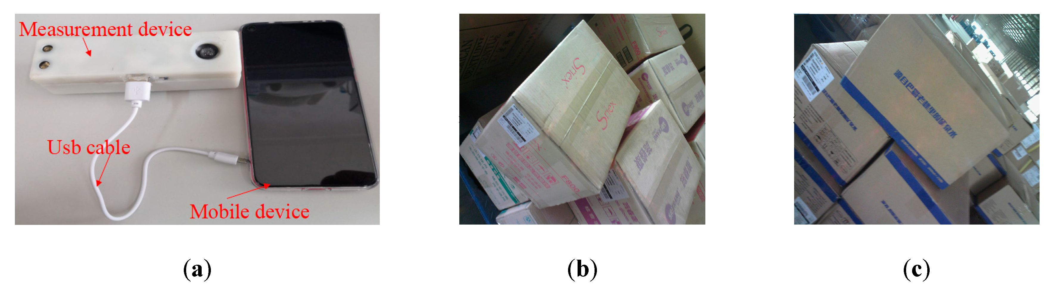
A hand-held visual sensor and online measurement system based on laser triangulation and deep learning technique for box dimension measurement are proposed.

(2)

A valid dataset of the laser-box images is created, and an effective structured edge detection and key point detection approach based on a Trimmed-HED network and straight-line processing are proposed.

(3)

An optimization method is proposed to achieve the robust calibration of the visual sensor.

This paper is organized as follows: in Section 2, the box dimension measurement system is introduced briefly. In Section 3, the measurement algorithmic procedure, the visual sensor’s calibration method, laser-box image processing, and detection algorithms for laser stripes and key points are reported. In Section 4, the performance of the measurement system is analyzed. Finally, conclusions and future work are drawn.

2. Materials and Methods

The portable dimension measurement system for boxes proposed in this paper is shown in Figure 2. The system comprises a cross-line laser projector (power: 10 mW, wavelength: 670 nm), a high-resolution digital color camera, and a compact housing. Two laser stripes are projected from the laser projector, forming a cross-line laser stripe on the box face. The visible cross-line laser stripes in the laser-box images (Figure 3a) are captured by using a 2592 × 1944 pixel camera with 3.6 mm lens. The size of our portable visual sensor is 120 mm × 35 mm × 35 mm, thereby making the system suitable for portable box dimension measurement.

The system should take two laser-box images to measure the dimension of the box. Figure 4a shows the mutual position of the visual sensor and the standard box.

Figure 4b,c show the acquisition of the box images. Figure 4a shows the mutual position of the sensor and box, as well as the reference system adopted in the problem. The visual sensor projects cross laser beams onto the box forming cross stripes, which are captured in laser-box images by the camera for measurement. The metric information of the box is stored in the center lines of the laser strips. The values are directly expressed in mm with respect to a camera coordinate system centered on the device.

A visual sensor system has been designed to compute the dimension of the box and combine the detection of the inspected boxes’ structured edge map and 2D key points (Figure 3b) of the laser-box images with the calibrated visual sensor. The system workflow is presented in Figure 5, showing the application operation.

With the calibrated device, the two laser-box images of the adjacent faces of the box are captured by the system. The precise geometry of the structured edge of the box face is detected by the trimmed-HED network, and the 2D key points are detected by Hough transformation to the box’s silhouette edges. Then, the transformation from 2D image point to 3D space point of the key points on the images is used to fit the plane equations of the box face combined with the calibration parameters. Finally, the length of the face of the measured box is obtained by computing the 3D coordinates of the four vertices. The following sections describe the whole procedure in detail.

3. Proposed Algorithmic Procedure

3.1. Dimension Measurement Principle

We model boxes as parallelepipeds in the present work, although real boxes may present some bent edges, missing corners, and asymmetries. The dimension of a box can be computed from the 3D coordinates of these key points (Dot V₁, V₂, V₃, V₄, D₁, D₂, D₃, D₄ and O, as shown in Figure 6b) on the silhouette edges of the captured two laser-box images. Thus, before the dimension of the measured box can be obtained, the box silhouettes (Section 3.3.1) and the 2D coordinates of these key points (Section 3.3.2) should be extracted.

The camera and the cross-line laser are used to acquire laser-box images of the measured box, forming a cross-line laser strip line embedding the profile structured edge information of the box face, as shown in Figure 6b. If the parameter equation of the laser plane and the camera (in Section 3.2) is known, the equations of the box face can be computed by intersecting the image rays with the laser planes. Thus, the 3D coordinates of the key points can also be obtained easily.

Here, we define the camera coordinate system as the fiducial coordinate system. The equation of the laser light planes that describe the location of the laser planes in the camera coordinate system is assumed as follows:

$$\{\begin{array}{c}{\mathrm{a}}_1{\mathrm{x}}_{\mathrm{c}}{+\mathrm{b}}_1{\mathrm{y}}_{\mathrm{c}}{+\mathrm{c}}_1{\mathrm{z}}_{\mathrm{c}}+1=0\\ {\mathrm{a}}_2{\mathrm{x}}_{\mathrm{c}}{+\mathrm{b}}_2{\mathrm{y}}_{\mathrm{c}}{+\mathrm{c}}_2{\mathrm{z}}_{\mathrm{c}}+1=0\end{array}$$

(1)

where a_i, b_i, and c_i, (i = 1, 2) are the coefficients of the two laser planes in our system.

Therefore, a camera is modeled via the usual pinhole model to describe the projection relation between the 3D object space and the 2D image [23]. Thus, as shown in Figure 6a, four coordinate systems are established. These systems include the image pixel coordinate system (unit: pixel), the image physical coordinate system (unit: mm), the camera coordinate system (unit: mm), and the world coordinate system (unit: mm). The relationship between a 3D point P(X_w,Y_w,Z_w) and its image projection P(u,v) is given by:

$$\mathrm{s}\left[\begin{array}{c}\mathrm{u}\\ \mathrm{v}\\ 1\end{array}\right]=\mathrm{A}\left[\mathrm{R},\mathrm{t}\right]\left[\begin{array}{c}{\mathrm{X}}_{\mathrm{w}}\\ {\mathrm{Y}}_{\mathrm{w}}\\ {\mathrm{Z}}_{\mathrm{w}}\\ 1\end{array}\right]\mathrm{with}\mathrm{A}=\left[\begin{array}{ccc}\mathsf{\alpha }& 0& {\mathrm{u}}_0\\ 0& \mathsf{\beta }& {\mathrm{v}}_0\\ 0& 0& 1\end{array}\right]$$

(2)

where s is an arbitrary scale factor, (R, t), called the extrinsic parameters, are the rotation matrix and translation vector, respectively, which relate the camera coordinate system to the world coordinate system, A is the camera intrinsic matrix, and (u₀,v₀) is the principal point in the image pixel coordinate system. α and β are the scale factors in image u and v axes, and γ is the parameter describing the skew of the two image axes.

Equation (3) represents the transformation relationship of the point P between the camera coordinate system (X_c,Y_c,Z_c) and the image pixel coordinate system (u,v):

$$\left[\begin{array}{c}\mathrm{u}\\ \mathsf{\nu }\\ 1\end{array}\right]=\mathrm{A}\left[\begin{array}{c}{\mathrm{X}}_{\mathrm{c}}/{\mathrm{Z}}_{\mathrm{c}}\\ {\mathrm{Y}}_{\mathrm{c}}/{\mathrm{Z}}_{\mathrm{c}}\\ 1\end{array}\right]$$

(3)

Assuming the 3D coordinates (X_c,Y_c,Z_c) are also on the laser stripes and in the image pixel coordinate system, (u,v) could be derived from Equations (1) and (3):

$${\mathrm{X}}_{\mathrm{c}}{=\mathrm{Z}}_{\mathrm{c}}\frac{{(\mathrm{u}-\mathrm{u}}_0)}{\mathsf{\alpha }}$$

(4)

$${\mathrm{Y}}_{\mathrm{c}}{=\mathrm{Z}}_{\mathrm{c}}\frac{{(\mathrm{v}-\mathrm{v}}_0)}{\mathsf{\beta }}$$

(5)

$${\mathrm{Z}}_{\mathrm{c}}=\frac{{\mathrm{d}}_{\mathrm{i}}}{{\mathrm{a}}_{\mathrm{i}}}{(-\frac{{\mathrm{c}}_{\mathrm{i}}}{{\mathrm{a}}_{\mathrm{i}}}-\frac{{(\mathrm{u}-\mathrm{u}}_0)}{\mathsf{\alpha }}-\frac{{\mathrm{b}}_{\mathrm{i}}}{{\mathrm{a}}_{\mathrm{i}}}\frac{{(\mathrm{v}-\mathrm{v}}_0)}{\mathsf{\beta }})}^{-1}$$

(6)

Therefore, the 3D coordinates P(X_c,Y_c,Z_c) on the laser stripes in the camera coordinate system can be computed. Thus, all the 3D coordinates on the laser stripes in the camera coordinate system of the image can be obtained. Thus, with the 2D coordinates (Dot D₁, D₂, D₃, D₄, O) on the laser stripes of the box face, the box face plane equation can easily be fitted with the least-squares method in the camera coordinate system:

$${\mathrm{Ax}}_{\mathrm{c}}{+\mathrm{By}}_{\mathrm{c}}{+\mathrm{Cz}}_{\mathrm{c}}+1=0$$

(7)

where A, B, and C are the coefficients of the box face plane equation.

Thus, the 3D coordinates of these key points (V₁, V₂, V₃, and V₄) on the silhouette edges of the laser-box image could be derived from Equations (3) and (7). We assume that the 3D coordinates of the vertices of a box face (Dot V₁, V₂, V₃ and V₄) are V1(x_v1,y_v1,z_v1), V2(x_v2,y_v2,z_v2), V3(x_v3,y_v3,z_v3), and V4(x_v4,y_v4,z_v4), respectively. The length and the width of the box face can be computed as follows:

$$\begin{array}{ll}\mathrm{length}=1/2& (\sqrt{{{(\mathrm{x}}_{\mathrm{v}1}-{\mathrm{x}}_{\mathrm{v}2})}^2+{{(\mathrm{y}}_{\mathrm{v}1}-{\mathrm{y}}_{\mathrm{v}2})}^2+{{(\mathrm{z}}_{\mathrm{v}1}-{\mathrm{z}}_{\mathrm{v}2})}^2}+\hfill \\ & \sqrt{{{(\mathrm{x}}_{\mathrm{v}4}-{\mathrm{x}}_{\mathrm{v}3})}^2+{{(\mathrm{y}}_{\mathrm{v}4}-{\mathrm{y}}_{\mathrm{v}3})}^2+{{(\mathrm{z}}_{\mathrm{v}4}-{\mathrm{z}}_{\mathrm{v}3})}^2})\\ \mathrm{width}=1/2& (\sqrt{{{(\mathrm{x}}_{\mathrm{v}1}-{\mathrm{x}}_{\mathrm{v}4})}^2+{{(\mathrm{y}}_{\mathrm{v}1}-{\mathrm{y}}_{\mathrm{v}4})}^2+{{(\mathrm{z}}_{\mathrm{v}1}-{\mathrm{z}}_{\mathrm{v}4})}^2}+\hfill \\ & \sqrt{{{(\mathrm{x}}_{\mathrm{v}2}-{\mathrm{x}}_{\mathrm{v}3})}^2+{{(\mathrm{y}}_{\mathrm{v}2}-{\mathrm{y}}_{\mathrm{v}3})}^2+{{(\mathrm{z}}_{\mathrm{c}2}-{\mathrm{z}}_{\mathrm{v}3})}^2})\end{array}$$

(8)

Through the same strategy, the length’ and width’ of the box face can be obtained by processing any adjacent face of the box. Therefore, the height of the measured box can be expressed as

$$\mathrm{height}=\{\begin{array}{c}\begin{array}{c}\mathrm{width}{}^{\prime }\left(\min \right[(\mathrm{width}{}^{\prime }-\mathrm{width}),(\mathrm{width}{}^{\prime }-\mathrm{length}\left)\right]\hfill \\ \begin{array}{cc}\begin{array}{ccc}\begin{array}{ccc}& & \end{array}& & \end{array}& <\end{array}\min \left[\right(\mathrm{length}{}^{\prime }-\mathrm{width}),(\mathrm{length}{}^{\prime }-\mathrm{length}\left)\right])\end{array}\\ \begin{array}{l}\mathrm{height}{}^{\prime }\left(\min \right[(\mathrm{width}{}^{\prime }-\mathrm{width}),(\mathrm{width}{}^{\prime }-\mathrm{length}\left)\right]\hfill \\ \begin{array}{ccc}\begin{array}{ccc}& & \end{array}& \begin{array}{cc}& \end{array}& >\end{array}\min \left[\right(\mathrm{length}{}^{\prime }-\mathrm{width}),(\mathrm{length}{}^{\prime }-\mathrm{length}\left)\right])\end{array}\end{array}$$

(9)

The box volume can be computed as follows:

$$\mathrm{V}=\mathrm{width}\times \mathrm{length}\times \mathrm{height}$$

(10)

However, when we measure one box and the length of the two images is w × l, and we need to manually select the height of the box because the height cannot be satisfied with Equation (9) at this time. This is also a shortcoming of our system.

We have completed the box dimension measurement by taking two laser-box pictures via a visual sensor. However, we need to calibrate the visual sensor in advance as discussed in Section 3.2. A robust algorithm is also needed to detect the key points of the collected laser-box image precisely. In this work, the 2D coordinates of the key points are obtained by dealing with the structured edge map of the laser-box images, and the process will be described in detail in Section 3.3.2.

3.2. Automatic Calibration for the Visual Sensor

3.2.1. Parameter Calibration of the Visual Sensor

Camera resolution and measurement device calibration are factors that affect the accuracy of length measurement. The internal and external parameters of the system must be calibrated in advance to achieve sufficient accuracy for measurements from the visual sensor. The internal parameters are unique for a particular camera, and it includes the camera intrinsic matrix A and the distortion parameters k₁, k₂. The external parameter is the relative pose between the camera and the laser projector, and the two laser planes projected from the laser projector are defined as Equation (2) relative to our fiducial coordinate system. The external and internal parameters affect the geometric interpretation of its measurements.

In the camera calibration stage, the camera’s inherent parameters are calculated using Zhang’s method [26]. We employ a planar calibration pattern viewed simultaneously by the camera and laser projector. The laser light is emitted onto a planar calibration pattern and forms a light strip formed by the intersection of the laser plane and the calibration pattern plane. When collecting images, we move the camera to observe the calibrate pattern from different positions and ensure that the calibration board can fill the entire field of view. The internal parameters of the visual sensor, the camera’s extrinsic parameters R, t with respect to the calibrate pattern and the calibration plane equation of the calibrate pattern can be determined using Zhang’s method. Then, we extract all the intersections on the fitted line of the laser strip with the horizontal and vertical fitted lines of the feature points (Figure 7c) on the calibration pattern as calibration points on the laser strips. We collected N calibration images to obtain a sufficient number of calibration points on the laser stripe. In accordance with Equation (4), the 3D calibrated point’s coordinates P(X_c,Y_c,Z_c) of the 2D coordinates p(u,v) on the laser straight lines can be computed in the camera coordinate system. The objective function is the sum of the squares of the Euclidean distances from the calibration point to the laser plane, and the laser plane equations can be fitted via the Levenberg–Marquardt method [34,35] with these sufficient 3D calibration points:

$$\mathrm{F}(\mathrm{a},\mathrm{b},\mathrm{c})=\min \left({\displaystyle \sum _{\mathrm{k}=1}^{\mathrm{N}}(\frac{\left|{\mathrm{aX}}_{\mathrm{ck}}^{}{+\mathrm{bY}}_{\mathrm{ck}}^{}{+\mathrm{cZ}}_{\mathrm{ck}}^{}+1\right|}{\sqrt{{\mathrm{a}}^2{+\mathrm{b}}^2{+\mathrm{c}}^2}}}{)}^2\right)$$

(11)

where a, b, c are the parameters of the laser plane equation, N is the number of times the calibration pattern is placed, (X_ck,Y_ck,Z_ck) is the coordinate of the calibration points on the laser stripe, and N = 15, K = 1, 2, 3... N.

Figure 7a shows the general setup of our calibration approach. Figure 7b shows an example of a set of images used in the calibration, that is, 1300 mm × 1200 mm (having 19 × 19 corner pattern, with square size 57.0 mm used) and affixed to the glass. Figure 7d shows a laser plane fitted result during calibration.

3.2.2. Optimization for Calibration Parameters by Analyzing the Probability Distributions and Outlier Removal

In practical applications, the internal and external parameters of the same line structure visual device calculated via different calibration image sets will be different. The output of the camera and the laser projector exhibits noise, and the error estimates of the internal and external parameters will affect the final measurement. In the study, we assumed that it has a normal probability distribution in calibration. If calibration is performed at n times, the true value of these parameters can be restored.

For the improved application in engineering projects, a robust approach has been developed by iteratively dropping data parameters with excessive errors. The internal and external parameters are assumed to obey normal distribution, and expressed as N(m,σ²). Then, 99.7% of the data should lie inside the range [m − 3σ,m + 3σ]. When data lie outside the range, they can be culled given the large error in data compared with their true value. Therefore, the internal and extrinsic parameters of the visual sensor are reestimated in this work by using the remaining parameter sets that meet the ±3σ standards.

The proposed algorithm of the detail processing steps is as follows:

(1)

Acquire N calibration pattern images with laser stripes in different positions, and feature points and calibration points can be detected successfully from these images.

(2)

Select M images from the N calibration pattern images randomly in Step (1) to form a new image set, and there would be form CN M subsets image total, where CN M is a binomial coefficient.

(3)

The internal and external parameters of the visual sensor by these subsets image in Step (2) are calculated respectively with the method described above. A total of CN M sets of parameter data are generated to form a matrix of R^n×12, where each row in the matrix corresponds to the parameters (α,β,u₀,v₀,k₁,k₂,a₁,b₁,c₁,a₂,b₂,c₂) of the device calculated by each subset of images.

(4)

For each column parameter of the R^n×12 matrix in Step (3), calculate the mean mp and standard deviation σ_p via the method of maximum likelihood estimation of a normal distribution.

(5)

From the matrix parameters in Step (4), remove the row in which value of at least one parameter data (α,β,u₀,v₀,k₁,k₂,a₁,b₁,c₁,a₂,b₂,c₂) not lie inside the range of [m − 3σ,m + 3σ] to form a new matrix and repeat the operation of Step (4) for the new matrix until no data were removed from the new matrix.

(6)

The nature mean of each column of the final matrix in Step (5) is used as the final internal and external parameters of the visual sensor.

3.2.3. Experimental Verification and Accuracy Assessment

In the present study, calibration image sets M = 20, subset M = 15 are acquired, and CN M = 15,504. Similar to Zhang’s algorithm [26], the root mean square (RMS) projection errors between the real pixel coordinates (x_i,y_i) and the projected pixel coordinates (x project i,y project i) is calculated to assess the accuracy of the parameters:

$$\mathrm{Errors}=\sqrt{\frac{1}{{\mathrm{N}}_{\mathrm{featurepoints}}}{\displaystyle \sum _{\mathrm{i}=1}^{{\mathrm{N}}_{\mathrm{featurepoints}}}\left[{{(\mathrm{x}}_{\mathrm{i}}{-\mathrm{x}}_{\mathrm{i}}{}^{\mathrm{project}})}^2{+(\mathrm{y}}_{\mathrm{i}}{-\mathrm{y}}_{\mathrm{i}}{}^{\mathrm{project}}{)}^2\right]}}$$

(12)

The 10 sets of images are captured by our visual sensor device with the same calibration pattern in different orientations, each of which contains 25 calibration images to evaluate the accuracy of the proposed optimization algorithm. As shown in

Table 1. Accuracy assessment.

Measurement	Value
Mean RMS calculated using 10 sets of calibration pattern images	0.0568
RMS calculated using the true parameters	0.0215

, the average RMS of the 10 sets of image sets is calculated, and RMS is calculated by using the true internal and external parameters via the optimization method. The optimization algorithm proposed in this paper is effective and can obtain parameter data close to the true value.

Table 2. Calibration parameters of the visual sensor.

Parameters	Minimal Value	Maximal Value	True Value
α	2345.064	2363.778	2353.85
β	2358.273	2377.399	2367.13
u0	1244.827	1262.702	1254.69
v0	1007.973	1026.720	1018.36
k1	−0.0241551	−0.008247	−0.016697
k2	0.155643	0.3567460	0.232305
a1	0.00905	0.0160500	0.01021
b1	−0.013303	−0.009352	−0.010614
c1	0.0019727	0.002677	0.002166
a2	0.0095584	0.013372	0.010326
b2	0.009839	0.016606	0.010347
c2	0.0018325	0.0025490	0.002031

shows the minimum and maximum values for each parameter in the given original calibration image sets, and the corresponding true values ultimately calculated via the optimization algorithm. The proposed method provides a robust method for solving the calibration of line structure light visual sensors. The natural mean and standard deviation of the CN M sets of images after calibration are the internal and external parameters of the visual sensor, rather than a fixed result calibrated by a set of image sets. The proposed optimization algorithm is useful in engineering applications.

3.3. Image Processing for the Laser-Box Image

3.3.1. Detecting Structured Edge Map

The structured silhouette edges of the captured image should be obtained to compute the image 2D coordinates of the intersections and the vertices crossed by the laser plane and the edge of the box. The VGG16 [25] network is modified. This section presents an automated and effective method for detecting structured edge map and extracting straight lines from them with deep learning. In this section, we propose a novel trimmed-HED network. This structure has the best edge prediction results in our repeated tests. Our trimmed-HED model is improved from three aspects: (1) the laser-box image data set we built, and (2) the first two side-output layers of the HED cut to ignore the detail feature in the image, and (3) the loss function slightly simplified by calculating the fusion layer outputs only that can improve the edge map prediction coarse-to-fine structure progressively.

(1) Laser-box image dataset

The problems of structured edge map detection is solved by learning from diverse samples. In building the data set, the best-fitted rectangle is marked by manual manipulation. We labeled images with nine 2D coordinates on the laser-box image containing the four intersections (intersection of the edge of box face and laser line) and other four points (on the box face edge), and the ground truth is obtained by drawing the straight line of these 2D coordinates. Figure 8 shows the sample images and the ground-truth structured edge maps of our developed dataset.

Data augmentation is an effective method to generate sufficient training data for learning a robust deep network. We rotate the images to seven different angles (45°, 90°, 135°, 180°, 225°, 270°, and 315°). In total, our dataset comprises 96,000 training images and 500 testing images.

(2) Trimmed-HED network

Figure 9 shows an overview of the proposed trimmed-HED network structured edge detection. The original HED network was designed with five side-output layers and one fuse-output, and the final output was obtained through the weighted-fusion and average layer. HED and RCF indicate that the side-output layers in front of the network (low-level network) are focused on extracting the detail edges of the image, and the high-level network is focused on the extraction of the target contour. However, the overall structured edge of the box face and the laser straight line are the main concerns in the present work. Therefore, the trimmed-HED cut the first two side-output layers of HED.

The total cross-entropy loss in HED is updated via standard stochastic gradient descent by the sum of the loss function at the side outputs and the fusion layer, as shown in the following equation:

$${(\mathrm{W},\mathrm{w})}^{*}{=\mathrm{argmin}(\mathrm{L}}_{\mathrm{side}}(\mathrm{W},\mathrm{w}),{+\mathrm{L}}_{\mathrm{fuse}}(\mathrm{W},\mathrm{w},\mathrm{h}),)$$

(13)

where L (W,w,h) fuse denotes the loss function at the fusion layer and the L (W,w) side denotes the loss function at the side-output layer. W denotes the standard network layer parameters, w denotes the parameters of the side-output layers, and h indicates the fusion coefficient of each side output layer.

The entire network in HED was trained with weighted-fusion supervision and side-output layer supervision. Compared with the train with weighted-fusion supervision only, the edge map predictions are progressively coarse-to-fine, local-to-global when train both. However, in trimmed-HED, the train with weighted-fusion supervision only exhibits complete structural information, and the network can learn from the image. Therefore, our loss function in trimmed-HED becomes:

$${(\mathrm{W},\mathrm{w})}^{*}{=\mathrm{argmin}(\mathrm{L}}_{\mathrm{fuse}}(\mathrm{W},\mathrm{w},\mathrm{h}),)$$

(14)

The final edge map predictions (Youtput) can be computed by further aggregating these edge maps of the side-output layers and the weighted-fusion layer:

$${\widehat{\mathrm{Y}}}_{\mathrm{output}}{=\mathrm{Average}(\widehat{\mathrm{Y}}}_{\mathrm{fuse}}{,\widehat{\mathrm{Y}}}_{\mathrm{side}}^{\left(3\right)}{,\widehat{\mathrm{Y}}}_{\mathrm{side}}^{\left(4\right)}{,\widehat{\mathrm{Y}}}_{\mathrm{side}}^{\left(5\right)})$$

(15)

where the Y(3), Y(4), and Y(5) sides are the output of the side-output layer(3), the side-output layer(4), and the side-output layer(5), respectively.

The parameters of our networks include the mini-batch size (10), the learning rate (1e-3), the loss weight for each side-output (1), the weight decay (0.0002), and the number of training iterations (1e+5 divides learning rate by 10 after 1000).

The performance of the structured edge detection algorithm was evaluated using three standard measures: a fixed scale of the best F-measure on the data set (ODS), the best threshold for each image (OIS), and the average precision (AP). The trimmed-HED method was compared with the original HED method and the trimmed-HED (with/without deep supervision). The detailed experimental results are shown in

Table 3. Performance of network alternative architectures. The “without deep supervision” result is trained using Equation (14). The “with deep supervision” result is trained by Equation (13).

	ODS	OIS	AP
Original HED	0.490	0.566	0.539
Original HED (with our data set)	0.621	0.662	0.648
Trimmed-HED (with deep supervision)	0.753	0.783	0.776
Trimmed-HED (without deep supervision)	0.803	0.816	0.809

. The results shown by original HED in Table 3 are unsatisfactory and are expected because a dataset not specifically designed to solve the problem in this study was used. Compared with the results shown in the first two rows of Table 3, creating a standard dataset has an advantage on the success of this study. Thus, compared with the original HED and original HED with our dataset, ODS increased by 0.131, OIS increased by 0.096, and AP increased by 0.109. The trimmed-HED without deep supervision achieved the best result in detecting the structured edge map as shown in the experiment. The ODS of our model is 0.803, OIS is 0.816, and AP is 0.809.

Figure 10 shows a set of experimental renderings to observe the experimental results intuitively. Cols (c), (d), (e), and (f) show that the original HED outputs have false edges, which are distributed in the overall image. The trimmed-HED with deep supervision obtained a satisfactory effect compared with the other three networks, indicating that the approach had high reliability in structured edge detection of laser-box image.

3.3.2. Detecting 2D Key Points via the Hough Transformation

The structured edge map was extracted from the laser-box images, which was based on the proposed deep learning network. And the structured edge map shows the four edges of the box face measured and the projected intersecting laser lines. The straight lines should be extracted and their intersections in the structured edge maps to locate the 2D coordinates of these key points. In this work, the three steps were performed as follows:

Step 1.

The Hough line transform was used to detect the straight line ρ = xcos(θ) + ysin(θ) from the structured edge maps of the laser-box images and transformed from each straight line to the parameter space.

Step 2.

(ρ,θ) for many cells was quantified, and an accumulator for each interval area was created. For every pixel (x,y) in the structured edge map of the laser-box image, the quantized value (ρ,θ) was computed, and the nearly collinear line segments were clustered by a suitable threshold for ρ and θ.

Step 3.

The image space lines composed of the N first (ρ,θ) in Step 2 were obtained and fitted via the LSM. N is 6 in this study.

Figure 11 presents the key point detection results of the raw input images. The Opencv function cornerSubPix() was used to detect the Sub-pixel coordinates of these key points. The parameter winSize in this function, representing the radius of the search window, was set to 4 × 4 in this study. For each image, the detected 2D coordinates of the key points are shown in the raw images in Figure 11c to illustrate the experimental results intuitively. The location of key points was precisely detected by our proposed approach.

4. Experimental Results

The overall measurement system is shown in Figure 1. The vision sensor is connected to a mobile device via a USB cable. The effective measurement distance with respect to the vision sensor is 0.1–2.5m. The normal working environmental temperature of the system is −15 °C–60 °C. Before these experiments, the calibration parameters of the vision sensor were calibrated in advance with the method described in Section 3.2. The detailed parameters are shown in Table 2.

A few operational experiments under varying operating conditions were carried out to evaluate the performance and effectiveness of the proposed system and the validity of the corresponding algorithms derived above. Five experimental phases were conducted to evaluate system performance. (1) The relative angle of the boxes measured and the visual sensor was changed; (2) the distance between the visual sensor and boxes was changed; (3) systematic error and measurement uncertainty analyses experiments of the system were performed; (4) the measurement accuracy of the system on various boxes in different scenarios was verified; and (5) some online test experiments were performed.

4.1. Measurement Statistical Analysis Experimental of Varying Orientations of the Measurement Object

In this experiment, the robustness of the proposed system with varied box orientation with respect to the visual sensor was evaluated.

The visual sensor was placed at five different positions with different orientation, and the angles between the face of the measured and the z-axis of the reference system of the sensor (see Figure 4a) are 30°, 45°, 60°, 75°, and 90°, respectively.

In this experiment, estimated values are reported as the average of 30 experimental sessions on the same box (Figure 12a,b).

Table 4. Measurement performance with 30 times at five different orientations.

			Measurement at Different Angles (The Measurement Error (mm) in Brackets) [The Relative Error (%) in Square Brackets]
	Dim	Ground Truth	90°	75°	60°	45°	30°
(a)	W	190.0	190.0	189.3 (−0.7) [0.37%]	190.9 (+0.9) [0.47%]	191.1 (+1.1) [0.58%]	188.2 (−1.8) [0.95%]
	L	253.0	253.0	252.2 (−0.8) [0.32%]	251.8 (−1.2) [0.47%]	251.7 (−1.3) [0.51%]	254.9 (+1.9) [0.75%]
	H	400.0	400.0	400.9 (+0.9) [0.23%]	401.6 (+1.6) [0.40%]	401.9 (+1.9) [0.48%]	396.2 (−3.8) [0.95%]
(b)	W	320.0	320.0	320.6 (+0.6) [0.19%]	321.5 (+1.5) [0.47%]	321.6 (+1.6) [0.50%]	317.3 (−2.7) [0.84%]
	L	320.0	320.0	320.9 (+0.9) [0.28%]	319.6 (−0.4) [0.13%]	321.4 (+1.4) [0.44%]	318.5 (−1.5) [0.47%]
	H	620.0	620.0	621.3 (+1.3) [0.21%]	622.4 (+2.4) [0.39%]	617.5 (−2.5) [0.4%]	623.5 (+3.5) [0.56%]

shows the measurement results in terms of W, L, and H of the boxes.

As shown in Figure 13, the average absolute errors (L, W, and H of the two standard boxes) at 90°, 75°, 60°, 45°, and 30° were 0.867, 1.333, 1.633, 2.533, and 3.083, mm respectively, indicating that the orientation of the measured box with the visual sensor does not significantly affect the measurement results. However, at an angle of 90°, the system can obtain the best measurement results and achieved a 0.26% average relative error. The maximum error in the measurement results in the experiment is 3.8 mm, indicating that the measurement system has good applicability in practical measurement.

4.2. Measurement Statistical Analysis Experimental of the Changing Distance between the Visual Sensor and the Measured Box

The box was measured at five different distances from the visual sensor (dis1 = 0.8 m, dis2 = 1.2 m, dis3 = 1.6 m, dis4 = 2.0 m and dis5 = 2.4 m). W, L, and H of the boxes ((a), (b), (c), in Figure 14) were recorded, and the measurement error was computed with the relative error. The measurement results reported in this experiment are recorded in

Table 5. Measurements and errors versus the visual sensor and measured box distance.

Box	Dim	Ground Truth	Measurement at Three Box-Sensor Distances (mm) (The Measurement Error (mm) in Brackets) [The Relative Error (%) in Square Brackets.]
		/mm	800	1200	1600	2000	2400
(a)	W	750.0	750.5 (+0.5) [0.07%]	751.2 (+1.2) [0.16%]	747.7 (−2.3) [0.31%]	746.4 (−3.6) [0.48%]	744.6 (−5.4) [0.72%]
	L	495.0	494.8 (−0.2) [0.04%]	493.9 (−1.1) [0.22%]	496.1 (+1.1) [0.22%]	492.4 (−2.6) [0.53%]	490.4 (−4.6) [0.93%]
	H	330.0	330.4 (+0.4) [0.12%]	330.8 (+0.8) [0.24%]	329.0 (−1.0) [0.30%]	326.9 (−3.1) [0.94%]	333.9 (+3.9) [1.18%]
(b)	W	480.0	479.7 (−0.3) [0.63%]	480.8 (+0.8) [0.17%]	478.5 (−1.5) [0.31%]	483.0 (+3.0) [0.63%]	485.3 (+5.3) [1.10%]
	L	550.0	549.6 (−0.4) [0.07%]	550.6 (+0.6) [0.11%]	548.1 (−1.9) [0.35%]	552.4 (+2.4) [0.44%]	555.4 (+5.4) [0.98%]
	H	380.0	380.4 (+0.4) [0.11%]	379.1 (−0.9) [0.24%]	381.3 (+1.3) [0.34%]	382.6 (+2.6) [0.68%]	376.3 (−3.7) [0.97%]
(c)	W	450.0	450.5 (+0.5) [0.11%]	449.6 (−0.4) [0.09%]	451.4 (+1.4) [0.31%]	446.8 (−3.2) [0.71%]	454.8 (+4.8) [1.07%]
	L	650.0	649.1 (−0.9) [0.14%]	648.7 (−1.3) [0.20%]	648.4 (−1.6) [0.25%]	654.2 (+4.2) [0.65%]	655.8 (+5.8) [0.89%]
	H	350.0	350.1 (+0.1) [0.03%]	350.5 (+0.5) [0.14%]	348.8 (−1.2) [0.34%]	353.3 (+3.3) [0.94%]	346.7 (−3.3) [0.94%]

.

Figure 15 shows that at the distance sensor/boxes dis1, dis2, dis3, dis4, and dis5, the average absolute errors are 0.411, 0.844, 1.478, 3.111, and 4.689 mm, respectively. The following data from the table can be obtained: the error of the measured result increases with the increase of the measured distance. The maximum error of the measurement was 5.8 mm, which was kept within ±6 mm. The analyzed data show that our system has good accuracy in the normal measurement range of the box and vision sensor.

4.3. Stability Analysis and Evaluation of Uncertainty in the Measurement Experimental of the Measurement System

In this experiment, we evaluated the stability of the measurement system by making repetitive measurements of the box dimension. We used four standard boxes for measurement experimental to increase the credibility of the experiment. As shown in Figure 16a–d, the side length of the box is evenly distributed within the measurement interval of the measuring range, and L, W, and H of these standard boxes are 110.6 × 410.5 × 620.8, 390.8 × 240.6 × 530.7, 1110.7 × 750.8 × 880.9, and 690.7× 570.5 × 1500.0, respectively. The position of the box relative to the vision sensor in each shot was changed, so the measured value can be used to verify the measurement accuracy of the system. The experimental results (L, W, and H) of measurements for the standard boxes are shown in

Table 6. Stability analysis and the evaluation of uncertainty of the measurement system.

No.	W (a)	L (a)	H (a)	W (b)	L (b)	H (b)	W (c)	L (c)	H (c)	W (d)	L (d)	H (d)
1	110.5	410.1	620.3	391.6	239.9	530.6	1111.7	749.1	880.1	689.8	570.2	1500.9
2	109.4	409.6	620.4	390.2	240.1	529.1	1109.3	750.9	879.3	688.3	570.6	1501.2
3	107.6	411.6	619.6	390.5	241.9	531.2	1112.2	752.3	881.7	690.4	569.3	1499.7
4	110.2	411.8	621.1	389.4	240.7	531.7	1109.5	751.7	882.6	689.7	568.9	1496.5
5	110.3	410.6	620.2	388.3	238.6	529.6	1111.3	747.1	879.4	687.3	571.2	1502.3
6	109.8	408.3	621.8	390.6	239.9	528.7	1109.6	749.3	878.2	691.2	570.3	1505.3
7	109.2	410.3	617.6	391.5	238.9	529.1	1113.3	750.6	880.9	690.3	571.4	1496.8
8	110.7	408.1	619.7	391.4	241.6	530.1	1112.5	748.3	881.1	691.5	567.6	1498.3
9	110.6	409.5	618.3	388.6	240.1	527.6	1108.7	750.2	882.3	689.2	568.4	1502.4
10	111.3	410.2	621.8	391.2	240.9	528.9	1108.1	751.6	881.6	688.4	571.9	1497.9
11	111.5	411.3	617.4	390.4	241.5	529.6	1111.6	750.3	880.9	691.3	570.7	1500.8
12	110.1	412.3	620.5	389.2	238.6	530.8	1109.8	749.7	880.4	691.5	568.3	1496.3
13	109.6	408.6	619.7	388.6	239.2	530.7	1107.2	748.6	879.8	692.6	569.6	1498.4
14	108.3	409.9	621.9	389.2	240.5	531.8	1111.5	747.9	876.4	690.7	571.6	1503.6
15	109.2	410.7	619.5	391.7	241.1	528.4	1110.6	750.6	881.5	689.1	569.5	1502.7
Mean	109.88	410.19	619.98	390.16	240.23	529.86	1110.46	749.88	880.41	690.08	569.96	1500.20
Ave_Err	0.94	1.01	1.26	1.09	0.91	1.2	1.46	1.36	1.20	1.22	1.12	2.35
Std	1.01	1.21	1.36	1.15	1.03	1.20	1.68	1.44	1.57	1.39	1.26	2.68
μA	1.05	1.25	1.41	1.19	1.07	1.25	1.74	1.49	1.63	1.44	1.30	2.77

. The average estimated values were recorded as the average of 15 experimental sessions on the standard box with the best distance from the box-sensors. The stability analysis and the evaluation of uncertainty in the measurement experimental of the measurement system were evaluated by performs data statistics on the results of 15 measurements, and the mean (Mean), average absolute error (Ave_Err), standard deviation (Std), and the uncertainty of class A (μ_A) were calculated. The formula for calculating μ_A is as follows:

$${\mathsf{\mu }}_{\mathrm{A}}=\sqrt{\frac{{\displaystyle \sum _{\mathrm{i}=1}^{\mathrm{n}}{{(\mathrm{x}}_{\mathrm{i}}-\overline{\mathrm{x}})}^2}}{\mathrm{n}-1}}$$

(16)

where x_i is the measured data and $\overline{\mathrm{x}}$ is the mean of the measured data. n is the number of measurements, which is 15 in the experiment.

The standard deviation of the measurement results was analyzed in accordance with the actual length of the measured boxes. The maximum value of standard deviations was less than 2.68 mm, and the minimum value of the standard deviation was less than 1.01 mm, indicating that the box measurement system has reliable repeated measurement accuracy.

Ave_Err and μ_A in the computed dimensions increased as the measurement range of the system increased. This phenomenon is attributed to the relative error that tends to decrease as the distance of the visual sensor and box becomes small. Figure 17a,b show the average error distribution and the measurement uncertainty of the system of these 15 measurements and are consistent with the theoretical analysis. The maximum absolute error of the side length of the standard box is 4.7 mm. The measurement uncertainty of the measuring system is ±1.05 mm to ±2.77 mm within the range of 110–1500 mm, indicating that the measurement system has high reliability in actual measurement and strong practical application.

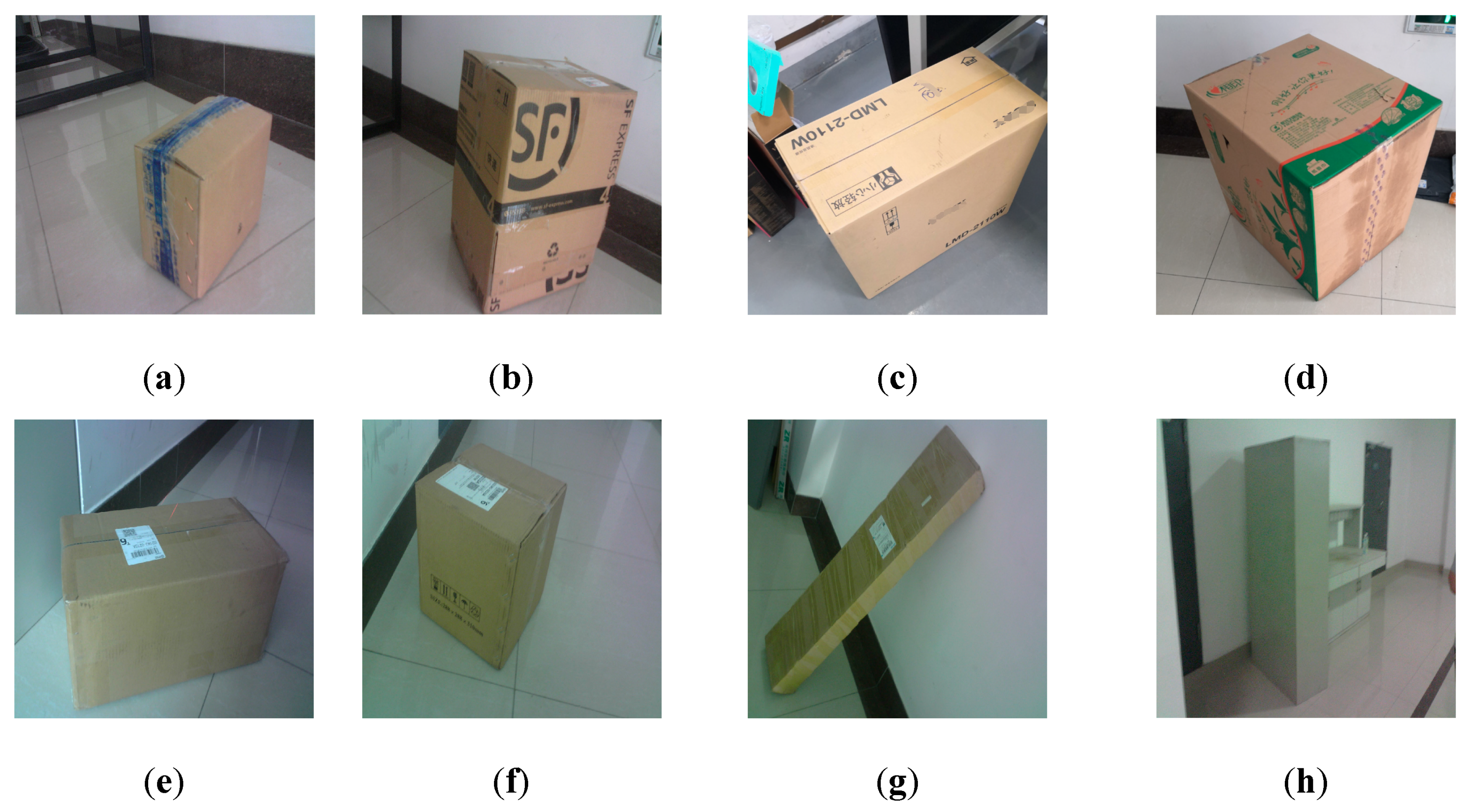
4.4. Measurement Statistical Analysis Experimental for Various Boxes in Different Scenarios

In this experiment, eight different boxes in different scenarios were measured. Figure 18a shows a box with a red surface; Figure 18b shows a box with high reflective area on the surface, where the reflective area would affect the imaging of the laser stripes in the image; Figure 18c shows a box with an ideal state; Figure 18d shows a box with a complex pattern and appendages on the surface; Figure 18e shows a box with surface variation (not an ideal plane); Figure 18g,h show the measurement of the target box with several boxes positioned in one plane. Figure 18f,g show the measurement of the same box in different scenarios. The raw laser-box image, the edge map, and the key points measured by the system are listed in

Table 7. Measurement result for various boxes in different scenarios, and the measurement error (mm) in brackets.

No.	(a)		(b)		(c)		(d)
Box
Edge map
Key points
Results	L: 99.5 (−0.5) W: 220.6(+0.6) H: 349.6(−0.4)		L: 301.2(+0.6) W: 368.3(−2.2) H: 428.5(−1.5)		L: 282.4(+0.4) W: 291.1(+1.1) H: 318.2(+2.2)		L: 294.2(+1.2) W: 312.3(+2.3) H: 349.8(−0.2)
No.	(e)		(f)		(g)		(h)
Box
Edge map
Key points
>Results	L: 256.3(+1.3) W: 500.6 (−9.4) H: 811.3(+11.3)		L: 172.3(+1.8) W: 222.7(+2.1) H: 332.6(+2.1)		L: 170.1(−0.4) W: 221.9(+1.3) H: 331.5(+1.0)		L: 319.9(−0.1) W: 318.3(−1.7) H: 623.8(+3.8)

. The width W, length L, height H of the box, and the absolute errors are recorded in brackets. The experimental results were analyzed and the following results were obtained: box (c) is an ideal box, with excellent performance in measurement results. The measurement results of boxes (a) and (d) indicate that the color characteristics on the surface of the box and the complexity of the pattern have no effect on the dimensional measurement of the box. The measurement results of box (b) show that the system is slightly negatively affected by the optical quality of the surface, thereby affecting key point detection and length measurement. The absolute measurement error of the L, W, and H of the box (e) are 1.3, 9.3, and 11.3 mm, respectively. For the measurement results of the box (e), although the maximum error result is 11.3 mm, our algorithm has a good effect on the edge and key point detection of such a box with an uneven surface. Such measurement results are acceptable for most logistics operations. The measurements of the boxes (f) and (g) are almost identical, suggesting that our system works well in complex situations, where multiple boxes are in the same plane. The measurement results of the box (h) also verify the effectiveness of the measurement system in a complex environment. Experimental results show that the system is slightly negatively affected by the color, the pattern, and the optical quality of the surface. However, a considerable measurement error was detected when a box with an uneven surface was detected.

Therefore, the experimental results show that the network designed in this paper can provide accurate positioning of the key point in the laser-box image even in the complex environment of multiple boxes. The measurements in Table 7 show that the errors of the side length of the box are between −2.2–+3.8 mm (excluding box (e) with irregular surfaces). This finding shows that the system we designed has a wide range of applicability.

4.5. Measurement Result in Real Applications

We also experimented on eight different boxes (Figure 19) in normal work conditions to validate the accuracy and reliability of the measurement system.

Table 8. Working online test.

No.	Actual Length/mm	Measured Length/mm	Length Error/mm	Relative Error of Length (%)	Volume Error/m3	Relative Error of Volume (%)
(a)	250.5	250.3	−0.2	0.079%	−0.00019	0.476%
	350.8	350.1	−0.7	0.199%
	454.6	453.7	−0.9	0.197%
(b)	560.5	561.6	+1.1	0.196%	0.000130	0.125%
	430.5	431.3	+0.8	0.185%
	430.5	429.4	−1.1	0.255%
(c)	400.0	402.3	+2.3	0.575%	0.000175	0.488%
	450.0	452.1	+2.1	0.466%
	200.0	198.9	−1.1	0.550%
(d)	520.0	523.6	+3.6	0.690%	0.000193	0.164%
	440.0	438.3	−1.7	0.386%
	515.0	513.6	−2.4	0.466%
(e)	220.4	220.0	−0.4	0.181%	−0.00012	0.451%
	300.7	299.4	−1.3	0.432%
	430.5	431.2	+0.7	0.162%
(f)	288.0	288.1	+0.1	0.034%	−0.00001	0.039%
	288.0	287.6	−0.4	0.138%
	310.0	310.2	+0.2	0.064%
(g)	1350.0	1354.5	+4.5	0.333%	0.000450	0.673%
	330.0	329.8	−0.2	0.060%
	150.0	150.6	+0.6	0.400%
(h)	1800.0	1807.6	+7.6	0.422%	0.003262	0.503%
	900.0	904.8	+4.8	0.533%
	400.0	398.2	−1.8	0.450%

shows the experimental results of measurements for eight standard boxes. The absolute error and the relative error of the measurement results were analyzed in accordance with the actual volumes and length of the measured boxes. The data in Table 8 indicate that the maximum relative error of length in the experiment was 0.575%, and the maximum measurement error of the length was 7.6mm, indicating good dimension measurement accuracy of the system.

5. Conclusions

A portable online dimension measurement system for boxes is required by the logistics industry to meet the challenging demands of intelligent logistics. In this work, the proposed dimension measurement system takes advantage of 3D reconstruction of box vertices to provide online dimension measurement. The system is based on laser triangulation and deep learning technology via a cross-line laser stripe cast onto the adjacent face of the box to be inspected. This method can accurately compute the 3D dimensions of boxes in adverse environmental conditions. The 2D coordinates of the key point in the laser-box images are detected using a novel end-to-end deep learning network with excellent performance. An effective optimization algorithm for structured light vision calibration was presented in which the camera intrinsic and extrinsic parameters of the device were improved by maximum likelihood estimation based on probability distribution. Experimental results show that the physical design for the proposed visual sensor is rational and the dimension measurement of box is effective. Our approach is readily applicable by future automated systems, which can integrate box targeting with the measurement method presented here. In the future, our work will continue to focus on the study of an intelligent and portable online box dimension measuring equipment system.

References

1. Georgousis, S.; Stentoumis, C.; Doulamis, N.; Athanasios, V. A Hybrid Algorithm for Dense Stereo Correspondences in Challenging Indoor Scenes. In Proceedings of the IEEE International Conference on Imaging Systems and Techniques, Chania, Greece, 4–6 October 2016; pp. 460–465. [Google Scholar]
2. Mustafah, Y.; Noor, R.; Hasbi, H. Stereo vision images processing for real-time object distance and size measurements. In Proceedings of the International Conference on Computer and Communication Engineering, Kuala Lumpur, Malaysia, 22–27 May 2012; pp. 659–663. [Google Scholar]
3. al Muallim, M.; Küçük, H.; Yılmaz, F.; Kahraman, M. Development of a dimensions measurement system based on depth camera for logistic applications. In Eleventh International Conference on Machine Vision; International Society for Optics and Photonics: Bellingham, WA, USA, 2018; Volume 11041, p. 110410. [Google Scholar]
4. Park, H.; Messemac, A.; Neveac, W. Box-Scan: An efficient and effective algorithm for box dimension measurement in conveyor systems using a single RGB-D camera. In Proceedings of the 7th IIAE International Conference on Industrial Application Engineering, Kitakyushu, Japan, 26–30 March 2019. [Google Scholar]
5. Ferreira, B.; Griné, M.; Gameiro, D. VOLUMNECT: Measuring volumes with Kinecttm. Int. Soc. Opt. Eng. 2014, 9013, 901304. [Google Scholar]
6. Leo, M.; Natale, A.; Del-Coco, M.; Carcagnì, P.; Distante, C. Robust estimation of object dimensions and external defect detection with a low-cost sensor. J. Nondestruct. Eval. 2017, 36, 17. [Google Scholar] [CrossRef]
7. Peng, T.; Zhang, Z.; Song, Y.; Chen, F.; Zeng, D. Portable System for Box Volume Measurement Based on Line-Structured Light Vision and Deep Learning. Sensors 2019, 19, 3921. [Google Scholar] [CrossRef] [PubMed] [Green Version]
8. Gao, Q.; Yin, D.; Luo, Q.; Liu, J. Minimum elastic bounding box algorithm for dimension detection of 3D objects: A case of airline baggage measurement. IET Image Process. 2018, 12, 1313–1321. [Google Scholar] [CrossRef]
9. Noll, R.; Krauhausen, M. Online laser measurement technology for rolled products. Ironmak. Steelmak. 2008, 35, 221–227. [Google Scholar] [CrossRef]
10. Zhang, L.; Sun, J.; Yin, G.; Zhao, J.; Han, Q. A cross structured light sensor and stripe segmentation method for visual tracking of a wall climbing robot. Sensors 2015, 15, 13725–13751. [Google Scholar] [CrossRef] [PubMed] [Green Version]
11. Appia, V.; Pedro, G. Comparison of fixed-pattern and multiple-pattern structured light imaging systems. Proc. SPIE 2014, 8979. [Google Scholar] [CrossRef]
12. Molleda, J.; Usamentiaga, R.; García, D.; Bulnes, F.; Ema, L. Shape measurement of steel strips using a laser-based three-dimensional reconstruction technique. IEEE Trans. Ind. Appl. 2011, 47, 1536–1544. [Google Scholar] [CrossRef]
13. Zhang, H.; Ren, Y.; Liu, C.; Zhu, J. Flying spot laser triangulation scanner using lateral synchronization for surface profile precision measurement. Appl. Opt. 2014, 53, 4405–4412. [Google Scholar] [CrossRef]
14. Bieri, L.; Jacques, J. Three-dimensional vision using structured light applied to quality control in production line. Proc. SPIE 2004, 5457, 463–471. [Google Scholar] [CrossRef] [Green Version]
15. Li, Y.; Li, Y.; Wang, Q.; Xu, D.; Tan, M. Measurement and defect detection of the weld bead based on online vision inspection. IEEE Trans. Instrum. Meas. 2010, 59, 1841–1849. [Google Scholar]
16. Giri, P.; Kharkovsky, S.; Samali, B. Inspection of metal and concrete specimens using imaging system with laser displacement sensor. Electronics 2011, 6, 36. [Google Scholar] [CrossRef] [Green Version]
17. Giri, P.; Kharkovsky, S. Dual-laser integrated microwave imaging system for nondestructive testing of construction materials and structures. IEEE Trans. Instrum. Meas. 2018, 67, 1329–1337. [Google Scholar] [CrossRef]
18. Zhao, X.; Liu, H.; Yu, Y.; Xu, X.; Hu, W.; Li, M.; Ou, J. Bridge Displacement Monitoring Method Based on Laser Projection Sensing Technology. Sensors 2015, 15, 8444–8463. [Google Scholar] [CrossRef]
19. Zhou, P.; Ke, X.; Wang, D. Rail profile measurement based on line-structured light vision. IEEE Access 2018, 6, 16423–16431. [Google Scholar] [CrossRef]
20. Miao, H.; Xiao, C.; Wei, M.; Li, Y. Efficient Measurement of Key-Cap Flatness for Computer Keyboards with a Multi-line Structured Light Imaging Approach. IEEE Sens. J. 2019, 21, 10087–10098. [Google Scholar] [CrossRef]
21. Xie, S.; Tu, Z. Holistically-nested edge detection. In Proceedings of the IEEE International Conference on Computer Vision, Santiago, Chile, 7–13 December 2015; pp. 1395–1403. [Google Scholar]
22. Liu, Y.; Cheng, M.; Hu, X.; Wang, K.; Bai, X. Richer convolutional features for edge detection. In Proceedings of the IEEE conference on computer vision and pattern recognition, Honolulu, HI, USA, 21–26 July 2017; pp. 3000–3009. [Google Scholar]
23. Shen, W.; Wang, B.; Jiang, Y.; Wang, Y.; Yuille, A. Multi-stage multi-recursive-input fully convolutional networks for neuronal boundary detection. In Proceedings of the IEEE International Conference on Computer Vision, Venice, Italy, 22–29 October 2017; pp. 2391–2400. [Google Scholar]
24. He, J.; Zhang, S.; Yang, M.; Shan, Y.; Huang, T. Bi-Directional Cascade Network for Perceptual Edge Detection. In Proceedings of the IEEE Conference on Computer Vision and Pattern Recognition, Long Beach, CA, USA, 19 August 2019; pp. 3828–3837. [Google Scholar]
25. Simonyan, K.; Zisserman, A. Very deep convolutional networks for large-scale image recognition. arXiv 2014, arXiv:1409.1556v6. [Google Scholar]
26. Zhang, Z. A flexible new technique for camera calibration. IEEE Trans. Pattern Anal. Mach. Intell. 2000, 22, 1330–1334. [Google Scholar] [CrossRef] [Green Version]
27. Tsai, R. A versatile camera calibration technique for high-accuracy 3D machine vision metrology using off-the-shelf TV cameras and lenses. IEEE J. Robot. Autom. 1987, 3, 323–344. [Google Scholar] [CrossRef] [Green Version]
28. Heikkila, J. Geometric camera calibration using circular control points. IEEE Trans. Pattern Anal. Mach. Intell. 2000, 22, 1066–1077. [Google Scholar] [CrossRef] [Green Version]
29. Zhang, Q.; Pless, R. Extrinsic calibration of a camera and laser range finder (improves camera calibration). In Proceedings of the 2004 IEEE/RSJ International Conference on Intelligent Robots and Systems, Sendai, Japan, 28 September–2 October 2004; Volume 3, pp. 2301–2306. [Google Scholar]
30. Zhang, G.; Liu, Z.; Sun, J.; Wei, Z. Novel calibration method for a multi-sensor visual measurement system based on structured light. Opt. Eng. 2010, 49, 043602. [Google Scholar] [CrossRef]
31. Vasconcelos, F.; Barreto, J.; Nunes, U. A minimal solution for the extrinsic calibration of a camera and a laser-rangefinder. IEEE Trans. Pattern Anal. Mach. Intell. 2012, 34, 2097–2107. [Google Scholar] [CrossRef] [PubMed]
32. Dong, W.; Isler, V. A novel method for the extrinsic calibration of a 2D laser rangefinder and a camera. IEEE Sens. J. 2018, 18, 4200–4211. [Google Scholar] [CrossRef] [Green Version]
33. So, E.; Michieletto, S.; Menegatti, E. Calibration of a dual-laser triangulation system for assembly line completeness inspection. In Proceedings of the 2012 IEEE International Symposium on Robotic and Sensors Environments Proceedings, Magdeburg, Germany, 16–18 November 2012; pp. 138–143. [Google Scholar]
34. Marquardt, D. An algorithm for least-squares estimation of nonlinear parameters. J. Soc. Ind. Appl. Math. 1963, 11, 431–441. [Google Scholar] [CrossRef]
35. Press, W.; Teukolsky, S.; Vetterling, W. Numerical Recipes in C: The Art of Scientific Computing; Cambridge University Press: Cambridge, MA, USA, 1995; Volume 10, pp. 176–177. [Google Scholar]
Figure 1. (a) Measurement device (b) and (c) the measured box in the distribution system.
Applsci 10 00026 g001
Figure 2. Measurement device.
Applsci 10 00026 g002
Figure 3. Display of dimension measurement system for the box. (a) laser-box image and (b) structured edge and key points.
Applsci 10 00026 g003
Figure 4. Measurement strategy. (a) The mutual position of the sensor and box; (b) The first laser-box image; (c) the second laser-box image, and the two laser-box image (b) and (c) the adjacent faces of the measured box.
Applsci 10 00026 g004
Figure 5. Workflow of the developed measurement system.
Applsci 10 00026 g005
Figure 6. (a) Perspective projection model of the visual sensor and (b) key points in the image.
Applsci 10 00026 g006
Figure 7. (a) Visual sensor calibration; (b) Calibration image; (c) Extracting the calibrate point on the laser stripes; (d) Laser plane fitting.
Applsci 10 00026 g007
Figure 8. Two example images and the ground-truth edge results for our dataset: (a,c) Input images; (b,d) are the ground-truth by human annotation of (a,c), respectively.
Applsci 10 00026 g008
Figure 9. Trimmed-HED network architecture. The green cubes represent the convolution layer, and the blue cubes represent the pooling layer. The prediction stage is a feed-forward network for generating initial predictions, and its architecture is divided into three stages. The final prediction output (a) is obtained by the weighted fusion of the side-output (3), side-output (4), and side-output (5).
Applsci 10 00026 g009
Figure 10. Comparison of original HED, HED with our dataset, trimmed-HED with/without deep supervision. (a) original image; (b) ground truth; (c) the results of original HED; (d) the results of HED with our dataset; (e) trimmed-HED with deep supervision; and (f) trimmed-HED without deep supervision.
Applsci 10 00026 g010
Figure 11. Detecting 2D key points. (a) Input image; (b) structured edge maps; (c) 2D coordinates of the key points detected through the straight lines.
Applsci 10 00026 g011
Figure 12. Two standard boxes with different dimensions used for testing: (a) 190.0 × 253.0 × 400.0; (b) 320.0 × 320.0 × 620.0.
Applsci 10 00026 g012
Figure 13. Average measurement error between the standard box and the measured result.
Applsci 10 00026 g013
Figure 14. Standard boxes with different dimension parameters, from (a) to (c). (a) 750.0 × 495.0 × 330.0; (b) 480.0 × 550.0 × 380.0; (c) 450.0 × 650.0 × 350.0.
Applsci 10 00026 g014
Figure 15. Relationship between the average absolute error with the object distance.
Applsci 10 00026 g015
Figure 16. Four standard boxes with different dimension parameters: (a) 110.6 × 410.5 × 620.8; (b) 390.8 × 240.6 × 530.7; (c) 1110.7 × 750.8 × 880.9; (d) 690.7 × 570.5 × 1500.0.
Applsci 10 00026 g016
Figure 17. (a) Relationship between the average error and the box length, (b) Relationship between the measurement uncertainty and the box length.
Applsci 10 00026 g017
Figure 18. Six boxes in different scenarios with different dimension parameters (mm): (a) 100.0 × 220.0 × 350.0; (b) 300.6 × 370.5 × 430.0; (c) 282.0 × 290.0 × 316.0; (d) 293.0 × 310.0 × 350.0; (e) 255.0 × 510.0 × 800.0; (f) 170.5 × 220.6 ×330.5; (g) 170.5 × 220.6 ×330.5; (h) 320.0 ×320.0 × 620.0.
Applsci 10 00026 g018
Figure 19. Eight boxes with different dimension: (a) 250.5 × 350.8 × 454.6; (b) 560.5 × 430.5 × 430.5; (c) 400.0 × 450.0 × 200.0; (d) 520.0 × 440.0 × 515.0; (e) 220.4 × 300.7 × 430.5; (f) 288.0 × 288.0 × 310.0; (g) 1350.0 × 330.0 × 150.0; (h) 1800.0 × 900.0 × 400.0.
Applsci 10 00026 g019